A new Diffuse-interface approximation of the Willmore flow

Abstract.

Standard diffuse approximations of the Willmore flow often lead to intersecting phase boundaries that in many cases do not correspond to the intended sharp interface evolution. Here we introduce a new two-variable diffuse approximation that includes a rather simple but efficient penalization of the deviation from a quasi-one dimensional structure of the phase fields. We justify the approximation property by a Gamma convergence result for the energies and a matched asymptotic expansion for the flow. Ground states of the energy are shown to be one-dimensional, in contrast to the presence of saddle solutions for the usual diffuse approximation. Finally we present numerical simulations that illustrate the approximation property and apply our new approach to problems where the usual approach leads to an undesired behavior.

1. Introduction

Curvature energies such as the elastica energy for plane curves or the Willmore functional for two-dimensional surfaces appear in a variety of applications in physics, biology or image processing. Diffuse approximations of such energies are part of many descriptions of phase transition problems and are used as a tool for numerical simulations of corresponding sharp interface problems. The most prominent diffuse approximation of the Willmore and elastica energy goes back to a suggestion of De Giorgi and builds on the well-known Cahn–Hilliard–Van der Waals functional that represents a perimeter approximation.

The approximation property of diffuse curvature energies is closely related to a supposed quasi one-dimensional structure of phase fields that describe moderate-energy states. For such structures the diffuse energies represent a certain averaging of the (sharp interface) bending energy of level lines. However, simulations [33, 16] with the standard diffuse approximations of the elastica or Willmore functional show a somehow non-intuitive behavior and the appearance of structures where diffuse interfaces cross. Level lines then carry an unbounded bending energy, and the generalized sharp interface energy of such structures (in the sense of an $L^{1}$ relaxation of the energy on smooth configurations) is infinite. Such behavior can be explained by the presence of (a wealth of) entire solutions of the stationary Allen–Cahn equation that deviate from the quasi one-dimensional structure. Such solutions have zero diffuse mean curvature everywhere and therefore are favored by the diffuse energies.

In many applications a preference for such structures is not consistent with the underlying physics or the intended behavior. Therefore several suggestions of alternative diffuse approximations have been proposed and analyzed. However, it seems that all present approaches come with a number of disadvantages and difficulties. In this contribution we introduce a new approximation that uses two phase field variables and penalizes a deviation from a quasi one-dimensional structure of the phase fields. For each variable a standard diffuse approximation is used, but with different choices of the double-well potential that determine the diffuse energy functionals. As long as both phase fields retain a quasi one-dimensional structure they are up to a simple transformation identical. This property motivates an additional energy contribution that penalizes a deviation from the desired behavior.

We justify this new approximation by a Gamma convergence result and show that zero energy states for the whole space problem are, in contrast to the classical De Giorgi approximation, necessarily one-dimensional. By a formal asymptotic expansion we show that a suitably rescaled $L^{2}$ gradient flow of the diffuse energy converges to the Willmore flow. Finally, we present numerical simulations that demonstrate the approximation property and consider applications of our approach in situations where the standard approximation leads to an undesired behavior.

In the following we fix a nonempty open set $\Omega\subset\mathbb{R}^{n}$. Let $\mathcal{M}$ denote the class of open sets $E\subset\Omega$ with $\Gamma=\partial E\cap\Omega$ given by a finite union of embedded closed $(n-1)$-dimensional $C^{2}$-manifolds without boundary in $\Omega$. We associate to such $\Gamma$ the inner unit normal field $\nu\mathrel{\mathop{\mathchar 58\relax}}\Gamma\to\mathbb{R}^{n}$, the shape operator $A$ with respect to $\nu$, and the principal curvatures $\kappa_{1},\dots,\kappa_{n-1}$ with respect to $\nu$. Finally we define the scalar mean curvature $H=\kappa_{1}+\ldots+\kappa_{n-1}$ and the mean curvature vector $\vec{H}=H\nu$, which implies that convex sets $E$ have positive mean curvature.

The Willmore energy [52] is then defined as

(1.1) $$\mathcal{W}(\Gamma)\mathrel{\mathop{\mathchar 58\relax}}=\frac{1}{2}\int_{\Gamma}H^{2}(x)\;\operatorname{d\!}\mathcal{H}^{n-1}(x).$$

Since the mean curvature vector $\vec{H}$ of a surface $\Gamma$ represents the $L^{2}$-gradient of the area functional $\mathcal{A}$ at $\Gamma$, we can characterize $\mathcal{W}$ as the squared $L^{2}$-norm of the gradient of $\mathcal{A}$. This observation suggests also an Ansatz for building diffuse approximations of the Willmore functional.

The $L^{2}$-gradient flow of $\mathcal{W}$ is called Willmore flow. For an evolving family of sets $(E(t))_{t\in(0,T)}$ in $\mathcal{M}$ with boundaries $\Gamma(t)=\partial E(t)\cap\Omega$ the velocity in direction of the inner normal field $\nu(t)$ is given by

(1.2) $$v(t)\, =\,-\Delta_{\Gamma(t)}{H}(t)+\frac{1}{2}H(t)^{3}-H(t)|A(t)|^{2},$$

on $\Gamma(t)$, where $|A(t)|^{2}=\kappa_{1}^{2}+\dots+\kappa_{n-1}^{2}$ denotes the squared Frobenius norm of the shape operator $A(t)$ and $\Delta_{\Gamma(t)}$ denotes the Laplace–Beltrami operator on $\Gamma(t)$.

In two dimensional space the Willmore functional for curves and the Willmore flow are better known as Eulers elastica functional and evolution of elastic curves. In this case (1.2) reduces to

(1.3) $$v(t)\, =\,-\Delta\kappa_{\Gamma(t)}(t)-\frac{1}{2}\kappa(t)^{3},$$

where $\kappa(t)$ denotes the curvature of $\Gamma(t)$. The Willmore flow of a single curve in the plane exists for all times [31] and converges for fixed curve length to an elastica, see also [21, 20] for further recent results on the topic.

Standard diffuse approximation

A well-known and widely used diffuse-interface approximation of the Willmore energy builds on the Cahn–Hilliard energy

(1.4) $$\mathcal{A}_{\varepsilon}(u)\mathrel{\mathop{\mathchar 58\relax}}=\int_{\Omega}\Big{(}\frac{\varepsilon}{2}|\nabla u|^{2}+\frac{1}{\varepsilon}W(u)\Big{)}\operatorname{d\!}\mathcal{L}^{n},$$

where $W$ is a suitable double-well potential and $u$ is a smooth function on $\Omega$.

The celebrated result by Modica and Mortola [41, 39] states that this functionals converge, in the sense of Gamma convergence with respect to the $L^{1}(\Omega)$ topology, to a constant multiple of the perimeter functional $\mathcal{A}$,

(1.5) $$\mathcal{A}_{\varepsilon}\to\sigma\mathcal{A},\quad\sigma=\int_{0}^{1}\sqrt{2W(s)}\,ds.$$

De Giorgi [24] conjectured that an approximation of the Willmore energy is given by the squared $L^{2}(\Omega)$-gradient of $\mathcal{A}_{\varepsilon}$, integrated against the diffuse area measure. In a slightly modified form that was introduced by Bellettini and Paolini [11] this leads to the functional

(1.6) $$\mathcal{W}_{\varepsilon}(u)\, \mathrel{\mathop{\mathchar 58\relax}}=\,\int_{\Omega}\frac{1}{2\varepsilon}\Big{(}-\varepsilon\Delta u+\frac{1}{\varepsilon}W^{\prime}(u)\Big{)}^{2}\operatorname{d\!}\mathcal{L}^{n},$$

that we consider in this paper as the standard diffuse approximation. The approximation property has been confirmed in a number of situations. Bellettini and Paolini [11] provided the Gamma-$\limsup$ estimate in arbitrary dimensions. To construct a recovery sequence for a given set $E\in\mathcal{M}$ two main ingredients are used: first the optimal transition profile that connects the wells of the double-well potential $W$, given by the unique solution $q\mathrel{\mathop{\mathchar 58\relax}}\mathbb{R}\to(0,1)$ of

$$-q^{\prime\prime}+W^{\prime}(q)=0\quad\text{ in }\mathbb{R},\quad q(-\infty)=0,\,q(\infty)=1,\,q(0)=\frac{1}{2}$$

and second the signed distance $d$ from $\Gamma$. Then, close to $\Gamma$ the approximating phase fields are given by $u_{\varepsilon}\approx q(d/\varepsilon)$. This is the quasi one-dimensional structure that one might expect for phase fields with low energy values. The $\liminf$ estimate necessary for the Gamma convergence of the diffuse Willmore approximations turned out to be much more difficult. It was proved under several additional assumptions in [9, 43] and finally for dimensions $n=2,3$ and for $C^{2}$-regular limit points in [46]. Note that in all these results the sum of diffuse area and diffuse Willmore functional was considered. However, the $\liminf$-estimate for the Willmore part itself holds as long as the diffuse surface area remains uniformly bounded.

Building on the approximation for the Willmore functional, the corresponding formal approximation of the Willmore flow is given by the $L^{2}(\Omega)$-gradient flow of $\mathcal{W}_{\varepsilon}$,

(1.7) $$\varepsilon\partial_{t}u\, =\,-\Delta\big{(}-\varepsilon\Delta u+\frac{1}{\varepsilon}W^{\prime}(u)\big{)}+\frac{1}{\varepsilon^{2}}W^{\prime\prime}(u)\big{(}-\varepsilon\Delta u+\frac{1}{\varepsilon}W^{\prime}(u)\big{)},$$

complemented by suitable boundary conditions for $u$ on $\partial\Omega$ and an initial condition for $u$ in $\Omega$. The convergence of the diffuse evolution towards the Willmore flow was shown by formal asymptotic expansions by Loreti and March [37] and by Wang [49]. Here a smooth evolution $(\Gamma(t))_{t\in(0,T)}$ of smooth surfaces and a phase field evolution $(u_{\varepsilon}(\cdot,t))_{t\in(0,T)}$ is considered that solves (1.7). If one assumes that the phase fields can be expanded around $(\Gamma(t))_{t}$, then the phase fields asymptotically have the expected one-dimensional structure and $(\Gamma(t))_{t\in(0,T)}$ evolves by Willmore flow.

The diffuse approximation of the Willmore flow and of more general curvature energies and flows are used for numerical simulations in a huge number of applications. Let us only mention here [29, 13, 30, 19, 50, 38, 27, 26, 33, 51, 15, 34]. For numerical treatment of Willmore flow in a sharp-interface approach, we refer to [4, 3, 2, 47, 25, 14, 32]. Moreover, level set techniques have been applied in order to simulate Willmore flow in [28, 12].

The diffuse Willmore approximation for non-smooth limit configurations

Numerical simulations

As mentioned above, it has been observed (see [33, 16] and the references therein) that, in particular in two dimensions, simulations based on the standard approximation lead to an in many cases undesired behavior: when diffuse interfaces meet they tend to produce transversal intersections of boundary layers.

This behavior is nicely illustrated if one starts from a number of equally distributed small circles in a unit square. The elastica functional of a ball is proportional to one over the radius, thus the balls start growing under the Willmore (elastica) flow and touch each other in finite time. From this point on there is no uniquely defined way how to continue the flow and the appropriate choice might depend on the present application. In any diffuse approximation the different balls will interact in a non-local way. The standard diffuse Willmore flow selects an evolution where diffuse interfaces start to flatten away from the touching points. Eventually, a perfect checkerboard pattern develops. In the simulations, the diffuse Willmore energy becomes extremely small in this situation.

The described behavior is in two dimensions not exceptional but rather generic for colliding phase interfaces that evolve subject to a descent dynamics of the standard diffuse Willmore energy. Another example occurs in the following application that considers two phases in a fixed volume that interact with a given inclusion. The phase is assumed to minimize an energy consisting of a bending contribution of the phase boundary and an adhesion energy (decreasing with increasing contact) between one of the phases and the inclusion. In section 6 we will study this application in more detail and apply our new diffuse approximation to this problem. Here we only consider the evolution in the case of the standard diffuse Willmore energy and a gradient descent method for the total energy, see Fig. 1.

Figure 1. Evolution of standard flow with an additional adhesion to inclusion contribution: Discrete phase-field $u_{h}$ for different times $t=0$, $t\approx 0.0077$, $t\approx 0.0237$, $t\approx 0.5914$. The white line indicates the boundary of the inclusion.

We clearly see that the evolution leads to configurations that do not correspond to an elastic behavior. In particular, introducing edge like phase boundaries should not be favorable.

Such examples have already motivated several alternative diffuse approximations. Before we comment on these and introduce our new approach we first will discuss particular entire solutions of the Allen–Cahn equation that promote the occurrence of intersecting phase boundaries in diffuse approximations.

Entire solutions of the stationary Allen–Cahn equation

The observed behavior and the occurrence of intersecting phase boundaries does not contradict the Gamma convergence for the diffuse Willmore energy, as all these results are restricted to $C^{2}$-regular interfaces and intersections are not considered. It is an open problem to characterize the sharp interface configurations that are in the domain of the Gamma limit of the diffuse Willmore approximation and to characterize the Gamma limit for non-smooth configurations. One could have guessed that the latter is given by the $L^{1}$-lower-semi-continuous relaxation of the elastica energy, which was characterized and investigated in [7, 10]. However, this is not the case as can be seen from the existence of saddle solutions of the stationary Allen–Cahn equation, which are characterized as entire solutions that have $\frac{1}{2}$ level lines given by the union of the coordinate axis in the plane and change sign from one quadrant to the other. The existence of such solutions was first proved by Dang, Fife and Peletier [22] and later extended in several directions [1, 17]. As a consequence of a simple spatial rescaling, this leads to a sequence $(u_{\varepsilon})_{\varepsilon}$ of zero energy states of the standard diffuse Willmore functional that converges to the characteristic function the first and third quadrant in the plane. Such a configuration on the other hand has been shown to have infinite energy with respect to the $L^{1}$-relaxation of the elastica energy [7]. From the observations above one may conjecture [16] that the Gamma limit of the diffuse Willmore functional is in fact given by a generalization of the Willmore functional in the sense of integral varifolds that behave additively on unions of one-dimensional sets. This is in coincidence with results in [53], where intersections of embedded curves are considered. The general case, however is open.

Alternative approximations that avoid intersecting phase boundaries

Several alternative diffuse approximations of the Willmore functional have been introduced that avoid the occurrence of intersecting phase boundaries. Bellettini [6] proposed such type of approximations for general geometric functionals. For the Willmore functional the squared mean curvature of the level sets of the phase field $u$ are integrated with respect to the diffuse area density,

(1.8) $$\hat{\mathcal{W}}_{\varepsilon}(u)\mathrel{\mathop{\mathchar 58\relax}}=\frac{1}{2}\int_{\Omega\setminus\{|\nabla u|=0\}}\Big{(}\nabla\cdot\frac{\nabla u}{|\nabla u|}\Big{)}^{2}\Big{(}\frac{\varepsilon}{2}|\nabla u|^{2}+\varepsilon^{-1}W(u)\Big{)}\operatorname{d\!}\mathcal{L}^{n}.$$

An alternative approximation of the elastica functional has been investigated by Mugnai [44], where the square integral of the diffuse second fundamental form is considered,

(1.9) $$\bar{\mathcal{W}}_{\varepsilon}(u)\mathrel{\mathop{\mathchar 58\relax}}=\frac{1}{2\varepsilon}\int_{\Omega}\left|\varepsilon D^{2}u-\varepsilon^{-1}W^{\prime}(u)\frac{\nabla u}{|\nabla u|}\otimes\frac{\nabla u}{|\nabla u|}\right|^{2}\operatorname{d\!}\mathcal{L}^{n}.$$

Finally, a third alternative has been introduced in [33]. There, the sum of the standard diffuse Willmore approximation and a suitable additional energy contribution was considered that penalizes the deviation of an appropriate rescaling of the diffuse mean curvature $w=-\varepsilon\Delta u+\frac{1}{\varepsilon}W^{\prime}(u)$ from the level set mean curvature $v=\nabla\cdot\frac{\nabla u}{|\nabla u|}$. More precisely, the additional penalty term is given

(1.10) $$\mathcal{P}_{\varepsilon}(u)\mathrel{\mathop{\mathchar 58\relax}}=\frac{1}{2\varepsilon^{1+\alpha}}\int_{\Omega}\left(w+\left(\varepsilon|\nabla u|\sqrt{2W(u)}\right)^{\frac{1}{2}}v\right)^{2}\operatorname{d\!}\mathcal{L}^{n},$$

where $0\leq\alpha\leq 1$.

In [6, 44, 33], for each of these proposals the Gamma-convergence to the $L^{1}$-lower semicontinuous envelope of the Willmore functional has been shown (for the $\liminf$ estimate a uniform bound on the diffuse area is assumed). In [33], for the third proposal numerical simulations have been included and a discussion of possible equilibrium shapes in specific situations where discussed. Brétin, Masnou and Oudet [16] compared the different approaches, showed the convergence of the corresponding $L^{2}$-gradient flows to the Willmore flow by formal asymptotic expansions, and discussed a number of numerical simulations.

All three alternative approximations have the advantage that the Gamma convergence to the $L^{1}$-lower semicontinuous envelope can be rigorously shown. On the other hand, using these approaches to numerically simulate the diffuse Willmore flow comes with several difficulties and obstacles in all three cases, e.g. (1.8),(1.10) include the level set mean curvature which can lead to numerical difficulties, especially due to its highly nonlinear nature and since it appears in corresponding flows to leading order. Moreover, (1.9) includes the full second derivative of $u$ leading to terms which do not have a divergence structure. We therefore introduce in this paper a new approach that is much more easy to implement for numerical simulations and that also seems to exclude non-generic configurations. As a partial justification of this observation, we prove below that zero energy states (’ground states’) necessarily have a one-dimensional structure and that Gamma-convergence in smooth points still holds.

2. A new diffuse Willmore flow avoiding intersections of phase boundaries

Doubling of variables.

The key idea is to consider two order parameters $u$, $v$ and diffuse Willmore energies $\mathcal{W}_{\varepsilon}^{(1)}(u)$ and $\mathcal{W}_{\varepsilon}^{(2)}(v)$, where

(2.1) $$\mathcal{W}_{\varepsilon}^{(j)}(u)\mathrel{\mathop{\mathchar 58\relax}}=\int_{\Omega}\frac{1}{2\varepsilon}\Big{(}-\varepsilon\Delta u+\frac{1}{\varepsilon}W_{j}^{\prime}(u)\Big{)}^{2}\operatorname{d\!}\mathcal{L}^{n}\quad j=1,2$$

with two different double well potentials $W_{1},W_{2}$. We then consider the corresponding optimal profile functions $q_{j}\mathrel{\mathop{\mathchar 58\relax}}\mathbb{R}\to(0,1)$,

(2.2) $$-q_{j}^{\prime\prime}+W_{j}^{\prime}(q_{j})=0,\quad\lim_{r\to-\infty}q_{j}(r)=0,\quad\lim_{r\to\infty}q_{j}(r)=1,\quad q_{j}(0)=\frac{1}{2}.$$

The profiles $q_{j}$ are strictly monotone increasing and characterized by

(2.3) $$q_{j}^{\prime}=\sqrt{2W_{j}(q_{j})},\quad q_{j}(0)=\frac{1}{2}.$$

We then define $\Phi\mathrel{\mathop{\mathchar 58\relax}}(0,1)\to(0,1)$ by $\Phi=q_{2}\circ q_{1}^{-1}$ and observe that $\Phi$ can be extended to a continuous strictly increasing and bijective function $\Phi\mathrel{\mathop{\mathchar 58\relax}}[0,1]\to[0,1]$. We obtain the properties

(2.4) $$q_{2}=\Phi(q_{1}),\qquad\Phi^{\prime}(q_{1})=\frac{q_{2}^{\prime}}{q_{1}^{\prime}}$$

and $\Phi\in C^{\infty}((0,1))$ for smooth double-well potentials $W_{j}$, $j=1,2$.

We remark that $2W_{2}(q_{2})=(q_{2}^{\prime})^{2}=\Phi^{\prime}(q_{1})^{2}(q_{1}^{\prime})^{2}=2\Phi^{\prime}(q_{1})^{2}W_{1}(q_{1})$, which yields

(2.5) $$W_{2}\circ\Phi=(\Phi^{\prime})^{2}W_{1},\qquad W_{2}^{\prime}\circ\Phi=2\Phi^{\prime\prime}W_{1}+\Phi^{\prime}W_{1}^{\prime}$$

Finally, we define $\Psi\mathrel{\mathop{\mathchar 58\relax}}=\Phi^{-1}$.

For given $W_{1},W_{2}$ the transformation $\Phi$ can be determined from (2.3), which gives

(2.6) $$\int_{\frac{1}{2}}^{\Phi(r)}\big{(}2W_{2}(s))^{-\frac{1}{2}}\,ds=\int_{\frac{1}{2}}^{r}\big{(}2W_{1}(s))^{-\frac{1}{2}}\,ds.$$

The motivation of our approach is that for quasi one-dimensional configurations $u,v$ with nearly optimal energy with respect to the diffuse approximations $\mathcal{W}_{\varepsilon}^{(1)}$ and $\mathcal{W}_{\varepsilon}^{(1)}$, respectively, the function $v$ is very close to $\Phi(u)$. On the other hand, some discrepancy occurs if at least one of both is different from the generic one-dimensional structure. A penalization of such discrepancy prevents the phase fields from evolving to non-generic configurations.

More specifically we introduce for two functions $u,v$ an additional energy contribution

(2.7) $$\mathcal{P}^{(\varepsilon)}(u,v)\mathrel{\mathop{\mathchar 58\relax}}=\int_{\Omega}P\big{(}\Phi(u)-v\big{)}\operatorname{d\!}\mathcal{L}^{n},$$

where $P$ is some fixed continuous function $P\mathrel{\mathop{\mathchar 58\relax}}\mathbb{R}\to\mathbb{R}^{+}_{0}$ with $P(0)=0$ and $P>0$ on $\mathbb{R}\setminus\{0\}$.

Moreover, we choose a penalty parameter $M_{\varepsilon}\geq 0$ with $M_{\varepsilon}\to\infty$ for $\varepsilon\to 0$. The total energy then reads

(2.8) $$\mathcal{F}_{\varepsilon}(u,v) \mathrel{\mathop{\mathchar 58\relax}}=\mathcal{W}^{(1)}_{\varepsilon}(u)+\mathcal{W}^{(2)}_{\varepsilon}(v)+M_{\varepsilon}\mathcal{P}^{(\varepsilon)}(u,v)$$

$$=\int_{\Omega}\frac{1}{2\varepsilon}\Big{(}-\varepsilon\Delta u+\frac{1}{\varepsilon}W_{1}^{\prime}(u)\Big{)}^{2}\operatorname{d\!}\mathcal{L}^{n}+\int_{\Omega}\frac{1}{2\varepsilon}\Big{(}-\varepsilon\Delta v+\frac{1}{\varepsilon}W_{2}^{\prime}(v)\Big{)}^{2}\operatorname{d\!}\mathcal{L}^{n}$$

$$\qquad\qquad+M_{\varepsilon}\int_{\Omega}P(\Phi(u)-v)\operatorname{d\!}\mathcal{L}^{n}.$$

Choices of double-well potentials and penalty term.

We always require the following conditions of the double-well potentials $W_{1},W_{2}$ to be satisfied:

(2.9) $$W_{j}\in C^{2}(\mathbb{R}),\quad W_{j}(0)=W_{j}(1)=0,\quad W_{j}>0\text{ on }\mathbb{R}\setminus\{0,1\},W_{j}^{\prime\prime}(0),W_{j}^{\prime\prime}(1)>0.$$

A standard example that we in particular use in our numerical simulation is given by

$$W_{1}(r)=18r^{2}(1-r)^{2},\qquad W_{2}=4W_{1},$$

see Section 6.2 below for the properties that are induced by this choice.

For the penalty energy $\mathcal{P}^{(\varepsilon)}$ we choose $P(\Phi(u)-v)=(\Phi(u)-v)^{k}$ with an even number $k=2l$, $l\in\mathbb{N}$. We let $k=4$ in the numerical simulations below.

For the penalty parameter we assume that

(2.10) $$\big{(}|\log\varepsilon|q_{2}^{\prime}(|\log\varepsilon|)\big{)}^{k}\varepsilon|\log\varepsilon|M_{\varepsilon}\to 0(\varepsilon\to 0).$$

A particular choice that we consider in the asymptotic expansions and numerical simulations below is $M_{\varepsilon}=\varepsilon^{-2}M$.

Evolutions laws.

We prescribe a rescaled $L^{2}(\Omega)\times L^{2}(\Omega)$ gradient flow for the total energy $\mathcal{F}_{\varepsilon}$ from (2.8)

(2.11) $$\varepsilon\partial_{t}u =-\nabla_{u}\mathcal{F}_{\varepsilon}(u,v)=-\nabla_{u}\mathcal{W}^{(1)}_{\varepsilon}(u)-M_{\varepsilon}\nabla_{u}\mathcal{P}^{(\varepsilon)}(u,v),$$

(2.12) $$\varepsilon\partial_{t}v =-\nabla_{v}\mathcal{F}_{\varepsilon}(u,v)=-\nabla_{u}\mathcal{W}^{(2)}_{\varepsilon}(v)-M_{\varepsilon}\nabla_{v}\mathcal{P}^{(\varepsilon)}(u,v),$$

where $\nabla_{u},\nabla_{v}$ denote the $L^{2}(\Omega)$-gradients with respect to $u,v$ respectively.

We compute

(2.13) $$\nabla_{u}\mathcal{W}^{(1)}_{\varepsilon}(u) =\big{(}-\Delta+\frac{1}{\varepsilon^{2}}W_{1}^{\prime\prime}(u)\big{)}\big{(}-\varepsilon\Delta u+\frac{1}{\varepsilon}W_{1}^{\prime}(u)\big{)},$$

(2.14) $$\nabla_{u}\mathcal{W}^{(2)}_{\varepsilon}(u) =\big{(}-\Delta+\frac{1}{\varepsilon^{2}}W_{2}^{\prime\prime}(u)\big{)}\big{(}-\varepsilon\Delta u+\frac{1}{\varepsilon}W_{2}^{\prime}(u)\big{)},$$

(2.15) $$\nabla_{u}\mathcal{P}^{(\varepsilon)}(u,v) =-P^{\prime}(\phi(u)-v)\phi^{\prime}(u),$$

(2.16) $$\nabla_{v}\mathcal{P}^{(\varepsilon)}(u,v) =P^{\prime}(\phi(u)-v)$$

and derive the system of fourth order evolution equations

(2.17) $$\varepsilon\partial_{t}u =-\big{(}-\Delta+\frac{1}{\varepsilon^{2}}W_{1}^{\prime\prime}(u)\big{)}\big{(}-\varepsilon\Delta u+\frac{1}{\varepsilon}W_{1}^{\prime}(u)\big{)}+M_{\varepsilon}P^{\prime}(\phi(u)-v)\phi^{\prime}(u),$$

(2.18) $$\varepsilon\partial_{t}v =-\big{(}-\Delta+\frac{1}{\varepsilon^{2}}W_{2}^{\prime\prime}(v)\big{)}\big{(}\varepsilon\Delta u+\frac{1}{\varepsilon}W_{2}^{\prime}(v)\big{)}-M_{\varepsilon}P^{\prime}(\phi(u)-v).$$

3. Zero energy states in the whole space

In this section we consider $\Omega=\mathbb{R}^{n}$ and configurations with vanishing energy. For the standard diffuse Willmore energy we recall that there exist zero energy states that depend not only on one variable, such as specific entire solutions of the Allen–Cahn equation like the saddle solutions from [22].

In contrast, for our total energy we prove that zero energy states are always one-dimensional.

Theorem 3.1 (Ground states are one-dimensional).

Assume that the double-well potentials $W_{1},W_{2}$ satisfy (2.9), and that $\{\Phi^{\prime\prime}=0\}$ is a discrete set. Let $\varepsilon>0$, $\Omega=\mathbb{R}^{n}$ and consider $u_{\varepsilon},v_{\varepsilon}\in H^{2}_{\operatorname{loc}}(\mathbb{R}^{n})$, $|u_{\varepsilon}|,|v_{\varepsilon}|\leq 1$ with $\mathcal{F}_{\varepsilon}(u_{\varepsilon},v_{\varepsilon})=0$.

Then one of the following two alternatives hold:

1. $u_{\varepsilon},v_{\varepsilon}$ are constant with $W_{1}^{\prime}(u_{\varepsilon})=0$, $W_{2}^{\prime}(v_{\varepsilon})=0$ and $\Phi(u_{\varepsilon})=v_{\varepsilon}$.

2. There exist $\nu\in\mathbb{S}^{n-1}$ and $x_{0}\in\mathbb{R}^{n}$ with $u_{\varepsilon}(x)=q_{1}\big{(}(x-x_{0})\cdot\nu\big{)}$ and $v_{\varepsilon}(x)=q_{2}\big{(}(x-x_{0})\cdot\nu\big{)}$.

We remark that for the standard choices of $W_{1},W_{2}$, as given above, in the first case we have $u_{\varepsilon}=v_{\varepsilon}\in\{0,\frac{1}{2},1\}$.

Proof. The property $\mathcal{F}_{\varepsilon}(u_{\varepsilon},v_{\varepsilon})=0$ is equivalent to

(3.1) $$-\varepsilon\Delta u_{\varepsilon}+\frac{1}{\varepsilon}W_{1}^{\prime}(u_{\varepsilon})=0,\quad-\varepsilon\Delta v_{\varepsilon}+\frac{1}{\varepsilon}W_{2}^{\prime}(v_{\varepsilon})=0,\quad v_{\varepsilon}=\Phi(u_{\varepsilon}).$$

First we consider general $u_{\varepsilon},v_{\varepsilon}$ not necessarily satisfying (3.1) and let $\tilde{v}_{\varepsilon}\mathrel{\mathop{\mathchar 58\relax}}=\Phi(u_{\varepsilon})$. We obtain

$$\nabla\tilde{v}_{\varepsilon}=\Phi^{\prime}(u_{\varepsilon})\nabla u_{\varepsilon},\quad\Delta\tilde{v}_{\varepsilon}=\Phi^{\prime\prime}(u_{\varepsilon})|\nabla u_{\varepsilon}|^{2}+\Phi^{\prime}(u_{\varepsilon})\Delta u_{\varepsilon},$$

hence, using (2.5),

$$\frac{\varepsilon}{2}|\nabla\tilde{v}_{\varepsilon}|^{2}+\frac{1}{\varepsilon}W_{2}(\tilde{v}_{\varepsilon})=\Phi^{\prime}(u_{\varepsilon})^{2}\Big{(}\frac{\varepsilon}{2}|\nabla u_{\varepsilon}|^{2}+\frac{1}{\varepsilon}W_{1}(u_{\varepsilon})\Big{)},$$

and

$$-\varepsilon\Delta\tilde{v}_{\varepsilon}+\frac{1}{\varepsilon}W_{2}^{\prime}(\tilde{v}_{\varepsilon}) =-\varepsilon\Phi^{\prime}(u_{\varepsilon})\Delta u_{\varepsilon}-\varepsilon\Phi^{\prime\prime}(u_{\varepsilon})|\nabla u_{\varepsilon}|^{2}+\frac{1}{\varepsilon}\Big{(}2\Phi^{\prime\prime}(u_{\varepsilon})W_{1}(u_{\varepsilon})+\Phi^{\prime}(u_{\varepsilon})W^{\prime}_{1}(u_{\varepsilon})\Big{)}$$

(3.2) $$=\Phi^{\prime}(u_{\varepsilon})\Big{(}-\varepsilon\Delta u_{\varepsilon}+\frac{1}{\varepsilon}W_{1}^{\prime}(u_{\varepsilon})\Big{)}-2\Phi^{\prime\prime}(u_{1})\Big{(}\frac{\varepsilon}{2}|\nabla u_{\varepsilon}|^{2}-\frac{1}{\varepsilon}W_{1}(u_{\varepsilon})\Big{)}.$$

We now exploit (3.1). By a spatial rescaling $x\mapsto\varepsilon x$ we can restrict ourselves to the case $\varepsilon=1$ in the following. We then deduce from (3.1) and (3.2) that $u=u(\varepsilon\cdot)$ is an entire solution of the stationary Allen–Cahn equation,

(3.3) $$-\Delta u+W_{1}^{\prime}(u)=0$$

and that

(3.4) $$0=\Phi^{\prime\prime}(u)\Big{(}\frac{1}{2}|\nabla u|^{2}-W_{1}(u)\Big{)}.$$

From (3.3) and elliptic regularity theory we deduce that $u$ is smooth. Moreover, by [40] $\frac{1}{2}|\nabla u|^{2}-W_{1}(u)\leq 0$ and $u(x)=0$ or $u(x)=1$ for some $x\in\mathbb{R}^{n}$ implies that $u$ is constant in $\mathbb{R}^{n}$. It therefore is sufficient to consider the case $0<u<1$ on $\mathbb{R}^{n}$.

Define the set $A\mathrel{\mathop{\mathchar 58\relax}}=\{|\nabla u|^{2}\neq 2W_{1}(u)\}$. Since $\{\Phi^{\prime\prime}=0\}$ is discrete we have by (3.4) that $u$ is constant in each connected component of $A$. It follows that $\nabla u=0$, $\Delta u=0$ and, by (3.3), $W_{1}^{\prime}(u)=0$ almost everywhere in $A$. By (2.9) this in particular implies that $\kappa_{0}\leq u\leq 1-\kappa_{0}$ almost everywhere in $A$ for some $0<\kappa_{0}<1$.

Consider any point $x\in\mathbb{R}^{n}$ such that the Lebesgue density of the set $A$ in $x$ is not zero or one, $\theta^{n}(A,x)\not\in\{0,1\}$. Then we obtain sequences $(x_{k})_{k}$ and $(x_{k}^{\prime})_{k}$ that both converge to $x$ such that $x_{k}\in A$, $x_{k}^{\prime}\not\in A$. By the preceding argument we may also assume that $\kappa_{0}\leq u(x_{k})\leq 1-\kappa_{0}$, $\nabla u(x_{k})=0$ for all $k\in\mathbb{N}$, which implies $\frac{1}{2}|\nabla u(x)|^{2}-W_{1}(u(x))<0$. On the other hand $\frac{1}{2}|\nabla u(x_{k}^{\prime})|^{2}-W_{1}(u(x_{k}^{\prime}))=0$ for all $k\in\mathbb{N}$, hence $\frac{1}{2}|\nabla u(x)|^{2}-W_{1}(u(x))=0$, a contradiction.

Therefore, $\theta^{n}(A,x)\in\{0,1\}$ for all $x\in\mathbb{R}^{n}$ which shows that $A$ or $\mathbb{R}^{n}\setminus A$ have measure zero. The second alternative yields that $u$ is constant on $\mathbb{R}^{n}$ and satisfies the properties in item (1). Hence it remains to consider the first alternative, which implies that $\frac{1}{2}|\nabla u|^{2}-W_{1}(u)=0$ in $\mathbb{R}^{n}$. By a remark in [42] (see also [18]) we obtain that $u$ is one-dimensional. In fact, define $z\mathrel{\mathop{\mathchar 58\relax}}\mathbb{R}^{n}\to\mathbb{R}$ by $u=q_{1}(z)$. We then deduce from the properties of the optimal profile function that

$$0=\frac{1}{2}|\nabla u|^{2}-W_{1}(u)=\frac{1}{2}q_{1}^{\prime}(z)^{2}|\nabla z|^{2}-W_{1}(q_{1}(z))=W(q_{1}(z))\big{(}|\nabla z|^{2}-1\big{)},$$

hence $|\nabla z|=1$ on $\mathbb{R}^{n}$. This further implies that

$$0=-\Delta u+W_{1}^{\prime}(u)=q_{1}^{\prime\prime}(z)|\nabla z|^{2}-q_{1}^{\prime}(z)\Delta z+W_{1}^{\prime}(q_{1}(z))=q_{1}^{\prime}(z)\Delta z$$

in $\mathbb{R}^{n}$ and $z$ is harmonic, with uniformly bounded gradient. The Liouville Theorem then yields that $u$ is a polynomial of degree one. Since the gradient has unit length we finally deduce $u(x)=q_{1}\big{(}(x-x_{0})\cdot\nu\big{)}$ for some $x_{0}\in\mathbb{R}^{n}$, $\nu\in\mathbb{S}^{n-1}$. By $\Phi(u)=v$ and the properties of $\Phi$ we also obtain that $v(x)=q_{2}\big{(}(x-x_{0})\cdot\nu\big{)}$. ∎

4. $\Gamma$ convergence of the two variable Willmore approximation

As a consequence of [46] we obtain the $\Gamma$-convergence of our total energy to the Willmore energy for regular configurations and small space dimensions.

First we extend the definition of $\mathcal{F}_{\varepsilon}$ to the whole of $L^{1}(\Omega)\times L^{1}(\Omega)$ by setting $\mathcal{F}_{\varepsilon}(u,v)=\infty$ if $u$ or $v$ does not belong to $H^{2}_{\operatorname{loc}}(\Omega)$. Next, we introduce the following subset $\mathcal{M}$ of characteristic functions with smooth jump set,

$$\mathcal{M}\mathrel{\mathop{\mathchar 58\relax}}=\{u\in BV(\Omega;\{0,1\})\,\mathrel{\mathop{\mathchar 58\relax}}\,u=\mathcal{X}_{E},\,E\subset\joinrel\subset\Omega\text{ is an open set with $C^{2}$-regular boundary}\}.$$

Moreover we define a two-variable diffuse perimeter functional $\mathcal{A}_{\varepsilon}\mathrel{\mathop{\mathchar 58\relax}}L^{1}(\Omega)\times L^{1}(\Omega)\to\mathbb{R}^{+}_{0}\cup\{+\infty\}$ by

(4.1) $$\tilde{\mathcal{A}}_{\varepsilon}(u,v)\mathrel{\mathop{\mathchar 58\relax}}=\mathcal{A}_{\varepsilon}(u)+\mathcal{A}_{\varepsilon}(v)$$

if $u,v\in H^{1}_{\operatorname{loc}}(\Omega)$ and $+\infty$ else.

Finally we denote the sum of the surface tension coefficients associated to $W_{1},W_{2}$ by $\sigma\mathrel{\mathop{\mathchar 58\relax}}=\sigma_{1}+\sigma_{2}$ and define two-variable perimeter and Willmore functionals by

(4.2) $$\tilde{\mathcal{A}}(u,u) \mathrel{\mathop{\mathchar 58\relax}}=\sigma\mathcal{A}(u)\quad\text{ if }u\in BV(\Omega;\{0,1\}),$$

(4.3) $$\tilde{\mathcal{W}}(u,u) \mathrel{\mathop{\mathchar 58\relax}}=\sigma\mathcal{W}(u)\quad\text{ if }u\in\mathcal{M},$$

and by setting $\tilde{\mathcal{A}}$ and $\tilde{\mathcal{W}}$ to $+\infty$ on $\{(u,v)\in L^{1}(\Omega)^{2}\,\mathrel{\mathop{\mathchar 58\relax}}\,u\neq v\text{ or }u\not\in BV(\Omega;\{0,1\})\}$ and $\{(u,v)\in L^{1}(\Omega)^{2}\,\mathrel{\mathop{\mathchar 58\relax}}\,u\neq v\text{ or }u\not\in\mathcal{M}\}$, respectively.

Theorem 4.1 ($\Gamma$-convergence of approximations).

Let $n=2$ or $n=3$ and consider double-well potentials $W_{1},W_{2}$ and $P$ as above. Then

(4.4) $$\Gamma-\lim_{\varepsilon\to 0}\big{(}\mathcal{F}_{\varepsilon}+\mathcal{A}_{\varepsilon}\big{)}=\sigma\big{(}\tilde{\mathcal{W}}+\tilde{\mathcal{A}}\big{)}$$

holds in $\mathcal{M}\times\mathcal{M}$.

Proof. The $\Gamma$-convergence in Theorem 4.1 is equivalent to a $\Gamma$-$\liminf$ and a $\Gamma$-$\limsup$ statement that we prove in the next two propositions. ∎

Proposition 4.2 ($\liminf$-inequality.).

Let the assumptions of Theorem 4.1 hold and consider any sequence $(u_{\varepsilon},v_{\varepsilon})$ in $L^{1}(\Omega)^{2}$ with $u_{\varepsilon}\to u$, $v_{\varepsilon}\to v$ for some $u\in\mathcal{M}$, $v\in L^{1}(\Omega)$. Then

(4.5) $$\sigma\mathcal{W}(u)\leq\liminf_{\varepsilon\to 0}\mathcal{F}_{\varepsilon}(u_{\varepsilon},v_{\varepsilon})$$

holds and $u=v$ is satisfied if the right-hand side is finite.

Proof. It is sufficient to consider the case that the right-hand side of the inequality (4.5) is bounded by some $\Lambda>0$. Then in particular

$$\mathcal{W}_{\varepsilon}^{(1)}(u_{\varepsilon})+\mathcal{A}_{\varepsilon}^{(1)}(u_{\varepsilon})\leq\Lambda,\qquad\mathcal{W}_{\varepsilon}^{(2)}(v_{\varepsilon})+\mathcal{A}_{\varepsilon}^{(2)}(v_{\varepsilon})\leq\Lambda$$

holds. We deduce from [39] and [46] that

(4.6) $$\sigma_{1}\big{(}\mathcal{W}(u)+\mathcal{A}(u)\big{)} \leq\liminf_{\varepsilon\to 0}\mathcal{W}_{\varepsilon}^{(1)}(u_{\varepsilon})+\mathcal{A}_{\varepsilon}^{(1)}(u_{\varepsilon}),$$

(4.7) $$\sigma_{2}\big{(}\mathcal{W}(v)+\mathcal{A}(v)\big{)} \leq\liminf_{\varepsilon\to 0}\mathcal{W}_{\varepsilon}^{(2)}(v_{\varepsilon})+\mathcal{A}_{\varepsilon}^{(2)}(v_{\varepsilon}).$$

In addition, by Fatou’s lemma we also have

$$\int_{\Omega}P(\Phi(u)-v)\leq\liminf_{\varepsilon\to 0}\int_{\Omega}P\big{(}\Phi(u_{\varepsilon})-v_{\varepsilon}\big{)}\leq\liminf_{\varepsilon\to 0}\frac{1}{M_{\varepsilon}}\Lambda=0,$$

which implies $\Phi(u)=v$. Since on the other hand $u,v\in\{0,1\}$ almost everywhere and $\Phi(0)=0$, $\Phi(1)=1$ we obtain that $u=v$. Adding (4.6) and (4.7) we conclude that (4.5) holds. ∎

Proposition 4.3 ($\limsup$-inequality).

Let the assumptions of Theorem 4.1 hold and consider any $u\in\mathcal{M}$. Then there exists a sequence $(u_{\varepsilon},v_{\varepsilon})$ in $L^{1}(\Omega)^{2}$ with $u_{\varepsilon}\to u$, $v_{\varepsilon}\to u$ such that

(4.8) $$\sigma\mathcal{W}(u)\geq\limsup_{\varepsilon\to 0}\mathcal{F}_{\varepsilon}(u_{\varepsilon},v_{\varepsilon}).$$

Proof. Here we consider the standard construction of recovery sequences for the diffuse Willmore functional, see [11]. Let $u\in\mathcal{M}$, $u=\mathcal{X}_{E}$ with $E\subset\joinrel\subset\Omega$ open and $C^{2}$-regular boundary $\Gamma$. Denote by $d$ the signed distance function to $\Gamma$, taken positive inside $E$. Next let $r_{\varepsilon}\mathrel{\mathop{\mathchar 58\relax}}=\varepsilon|\log\varepsilon|$ and define $q^{(\varepsilon)}_{j}\mathrel{\mathop{\mathchar 58\relax}}\mathbb{R}\to[0,1]$ by

$$q^{(\varepsilon)}_{j}(r)\mathrel{\mathop{\mathchar 58\relax}}=\begin{cases}q_{j}(\varepsilon^{-1}r)\quad&\text{ if }0\leq r\leq r_{\varepsilon},\\ p_{j}^{(\varepsilon)}(\varepsilon^{-1}r)\quad&\text{ if }r_{\varepsilon}<r<2r_{\varepsilon},\\ 1\quad&\text{ if }r_{\varepsilon}\geq 2r_{\varepsilon},\\ 1-q_{j}(-r)\quad&\text{ if }r<0,\end{cases}$$

where the third order polynomial $p_{j}^{(\varepsilon)}$ is chosen such that $q^{(\varepsilon)}_{j}\in C^{1}(\mathbb{R})$.

The approximations $u_{\varepsilon}$, $v_{\varepsilon}$ are then defined by

$$u_{\varepsilon}(x)=q^{(\varepsilon)}_{1}(d(x)),\quad v_{\varepsilon}(x)=q^{(\varepsilon)}_{2}(d(x)).$$

The definition of $\Phi$ yields that $v_{\varepsilon}=\Phi(u_{\varepsilon})$ in $\{|d|\leq\varepsilon|\log\varepsilon|\}$ and $\{|d|\geq 2\varepsilon|\log\varepsilon|\}$. Moreover, by [11] we have

$$u_{\varepsilon}\to u,\quad v_{\varepsilon}\to v\qquad\text{ in }L^{1}(\Omega),$$

$$\mathcal{W}_{\varepsilon}^{(1)}(u_{\varepsilon})+\mathcal{A}_{\varepsilon}^{(1)}(u_{\varepsilon})\,\to\,\sigma_{1}\big{(}\mathcal{W}(u)+\mathcal{A}(u)),$$

$$\mathcal{W}_{\varepsilon}^{(2)}(v_{\varepsilon})+\mathcal{A}_{\varepsilon}^{(2)}(v_{\varepsilon})\,\to\,\sigma_{2}\big{(}\mathcal{W}(u)+\mathcal{A}(u)).$$

Therefore, it only remains to consider the penalty energy $\mathcal{P}^{(\varepsilon)}$. Since $\Phi(q_{1})=q_{2}$ and since $\Phi(0)=0$, $\Phi(1)=1$ we only have a contribution from the region $r_{\varepsilon}<|d|<2r_{\varepsilon}$, hence

$$\mathcal{P}^{(\varepsilon)}(u_{\varepsilon},v_{\varepsilon}) \leq\int_{\{r_{\varepsilon}<|d|<2r_{\varepsilon}\}}\big{(}\Phi(p_{1}^{(\varepsilon)}(\varepsilon^{-1}d(x)))-p_{2}^{(\varepsilon)}(\varepsilon^{-1}d(x))\big{)}^{k}$$

$$\leq\varepsilon\int_{\Gamma}\int_{\varepsilon^{-1}r_{\varepsilon}}^{2\varepsilon^{-1}r_{\varepsilon}}\big{(}\Phi(p_{1}^{(\varepsilon)}(r))-p_{2}^{(\varepsilon)}(r)\big{)}^{k}J(y,\varepsilon r)\,dr\,d\mathcal{H}^{n-1}(y)$$

$$\qquad+\varepsilon\int_{\Gamma}\int_{-2\varepsilon^{-1}r_{\varepsilon}}^{-\varepsilon^{-1}r_{\varepsilon}}\big{(}\Phi(p_{1}^{(\varepsilon)}(r))-p_{2}^{(\varepsilon)}(r)\big{)}^{k}J(y,\varepsilon r)\,dr\,d\mathcal{H}^{n-1}(y),$$

where $J(y,s)$ denotes the Jacobi factor for the transformation $\vartheta\mathrel{\mathop{\mathchar 58\relax}}\Gamma\times(-\delta,\delta)$, $\vartheta(y,s)=y+s\nu(y)$. By the $C^{2}$-regularity of $\Gamma$ we have $|J(y,s)|\leq C$. Therefore,

$$M_{\varepsilon}\mathcal{P}^{(\varepsilon)}(u_{\varepsilon},v_{\varepsilon}) \leq 2M_{\varepsilon}C\mathcal{A}(\Gamma)r_{\varepsilon}\max_{|\log\varepsilon|<|r|<2|\log\varepsilon|}\big{|}\Phi(p_{1}^{(\varepsilon)}(r))-p_{2}^{(\varepsilon)}(r)\big{|}^{k}$$

$$\leq C(\Gamma)M_{\varepsilon}r_{\varepsilon}\big{(}q_{2}(\varepsilon^{-1}r_{\varepsilon})-q_{2}(2\varepsilon^{-1}r_{\varepsilon})\big{)}^{k}\,\to\,0,$$

where we have used that $p_{1}^{(\varepsilon)}$ is monotone for $\varepsilon\ll 1$ and assumptions (2.10) on $M_{\varepsilon}$. ∎

5. Matched asymptotic expansions

We follow and modify [37], see also [49, 16] and the references therein. To perform the asymptotic expansion we make here a specific choice of the penalty term,

(5.1) $$M_{\varepsilon}=M\varepsilon^{-2},\qquad P(r)=\frac{1}{2l}r^{2l}\quad\text{ for some }l\in\mathbb{N},l\geq 2.$$

For the expansion we assume that the $\frac{1}{2}$-level set of the solution $u_{\varepsilon}(\cdot,t)$, $t\in(0,T)$ is given by a smooth evolution of smooth hypersurfaces $(\Gamma_{\varepsilon}(t))_{t\in(0,T)}$ such that at time $t$ the set $\Omega$ is the disjoint union of $\Gamma_{\varepsilon}(t)$, the open set $\Omega^{+}_{\varepsilon}(t)=\{u_{\varepsilon}(\cdot,t)>\frac{1}{2}\}$, and the open set $\Omega^{-}_{\varepsilon}(t)=\{u_{\varepsilon}(\cdot,t)<\frac{1}{2}\}$. For simplicity we assume that $\Omega^{+}_{\varepsilon}(t)\subset\Omega_{0}\subset\joinrel\subset\Omega$, which means that $\Gamma_{\varepsilon}(t)$ does not touch $\partial\Omega$, for all $t\in(0,T)$.

We then assume that $u_{\varepsilon}(\cdot,t)$ can be represented away from $\Gamma_{\varepsilon}(t)$ by the outer expansion

$$u_{\varepsilon}(x,t)=u^{(0)}(x,t)+\varepsilon u^{(1)}(x,t)+\varepsilon^{2}u^{(2)}(x,t)+\ldots$$

and in a small neighborhood of $\Gamma_{\varepsilon}(t)$ by

$$u_{\varepsilon}(x,t)=U^{(0)}(z,y,t)+\varepsilon U^{(1)}(z,y,t)+\varepsilon^{2}U^{(2)}(z,y,t)+\ldots,$$

where $z=\frac{d_{\varepsilon}(x,t)}{\varepsilon}$ with $d_{\varepsilon}\mathrel{\mathop{\mathchar 58\relax}}=\operatorname{dist}_{\varepsilon}(x,\Omega^{-}(t))-\operatorname{dist}_{\varepsilon}(x,\Omega^{+}(t))$ the signed distance function from $\Gamma_{\varepsilon}(t)$ and $y$ the projection of $x$ on the hypersurface $\Gamma_{\varepsilon}(t)$. A similar expansion, again with respect to $\Gamma_{\varepsilon}(t)$, $t\in(0,T)$, we assume for $v_{\varepsilon}$. Note that we do not prescribe that $v_{\varepsilon}(\cdot,t)=\frac{1}{2}$ on $\Gamma_{\varepsilon}(t)$.

Finally, we assume that $\Gamma_{\varepsilon}(t)$ converges to some smooth evolution of smooth hypersurfaces $(\Gamma(t))_{t\in(0,T)}$, more precisely that $d_{\varepsilon}=d_{0}+O(\varepsilon)$, where $d_{0}(\cdot,t)$ denotes the signed distance function from $\Gamma(t)$. We will see below that only the zero order $d_{0}$ and geometric quantities of $\Gamma(t)$ enter up to the relevant order. Therefore, we drop in the following the explicit notation of the $\varepsilon$-dependence of these quantities and for example write $d$ instead of $d_{\varepsilon}$.

Outer expansion

Since we assume that $M_{\varepsilon}=o(\varepsilon^{-3})$, the leading contributions from (2.17), (2.18) are of order $\varepsilon^{-3}$ and imply

$$W_{1}^{\prime\prime}(u^{(0)})W_{1}^{\prime}(u^{(0)})=W_{2}^{\prime\prime}(v^{(0)})W_{2}^{\prime}(v^{(0)})=0.$$

A solution consistent with the boundary conditions and with the expected transition layer structure is that away from $\Gamma(t)$

$$u^{(0)}=v^{(0)}=\begin{cases}1\quad&\text{ in }\Omega^{+}(t),\\ 0\quad&\text{ in }\Omega^{-}(t)\end{cases}$$

holds. Since $u^{(0)}=v^{(0)}$, also in the next $O(\varepsilon^{-2})$ order no contribution from the additional penalty term appears and as in [37] we deduce that $u^{(1)}=v^{(1)}=0$. Iterating this arguments we derive that $u^{(2)}=v^{(2)}=0$ and $u^{(3)}=v^{(3)}=0$.

Inner expansion

Here we also expand the diffuse mean curvatures

(5.2) $$\mu^{\varepsilon}_{1}=-\varepsilon\Delta u_{\varepsilon}+\frac{1}{\varepsilon}W_{1}^{\prime}(u_{\varepsilon}),\qquad\mu^{\varepsilon}_{2}=-\varepsilon\Delta v_{\varepsilon}+\frac{1}{\varepsilon}W_{2}^{\prime}(v_{\varepsilon})$$

in a neighborhood of $\Gamma(t)$. Since we expect an (at least) $L^{2}$-integrable mean curvature in the limit it is reasonable to prescribe that they do not have a contribution of order $\varepsilon^{-1}$ or higher, hence

$$\mu^{\varepsilon}_{1}=\mu_{1}^{(0)}+\varepsilon\mu_{1}^{(1)}+\varepsilon^{2}\mu_{1}^{(2)}+\ldots,\qquad\mu^{\varepsilon}_{2}=\mu_{2}^{(0)}+\varepsilon\mu_{2}^{(1)}+\varepsilon^{2}\mu_{2}^{(2)}+\ldots.$$

Since the Laplacian can be expanded in the new coordinates as

(5.3) $$\Delta=\frac{1}{\varepsilon^{2}}\partial^{2}_{z}+\frac{1}{\varepsilon}\Delta d\partial_{z}+\Delta_{y},$$

see for example [37, (2.11)], the conditions that $\mu^{\varepsilon}_{1,2}$ vanish to order $\varepsilon^{-1}$ yield

(5.4) $$0=-\partial^{2}_{z}U^{(0)}+W_{1}^{\prime}(U^{(0)})=-\partial^{2}_{z}V^{(0)}+W_{2}^{\prime}(V^{(0)}).$$

Together with the matching conditions $U^{(0)}(-\infty)=V^{(0)}(-\infty)=0$, $U^{(0)}(\infty)=V^{(0)}(\infty)=1$ and the compatibility condition $U^{(0)}(0,y,t)=\frac{1}{2}$, which is induced by the definition of $\Gamma(t)$, we obtain that $u_{\varepsilon},v_{\varepsilon}$ are to highest order described by the corresponding (shifted) optimal profiles,

$$U^{(0)}(z,y,t)=q(z),\qquad V^{(0)}(z,y,t)=w\big{(}z-z_{0}(y,t)\big{)},$$

where $z_{0}(y,t)\in\mathbb{R}$ and where we set $q=q_{1}$, $w=q_{2}$ to reduce the number of indices. We define the linear operators

$$L_{1}=-\partial^{2}_{z}+W_{1}^{\prime\prime}(q),\qquad L_{2}=-\partial^{2}_{z}+W_{2}^{\prime\prime}(w(\cdot-z_{0})),$$

use (5.4) and $\Delta d(x)=-H(y)-\varepsilon(\sum_{i=1}^{n-1}\kappa_{i}^{2})z+O(\varepsilon^{2})$, see [37], and obtain

(5.5) $$\mu^{\varepsilon}_{1}= \big{(}L_{1}U^{(1)}+Hq^{\prime}(z)\big{)}$$

$$+\varepsilon\big{(}L_{1}U^{(2)}+H\partial_{z}U^{(1)}+(\sum_{i=1}^{n-1}\kappa_{i}^{2})zq^{\prime}+\frac{1}{2}W_{1}^{\prime\prime\prime}(q)(U^{(1)})^{2}\big{)}$$

$$+\varepsilon^{2}\mu_{1}^{(2)}+O(\varepsilon^{3}),$$

where $q=q(z)$, $U^{(1)}=U^{(1)}(z,y,t)$, $U^{(2)}=U^{(2)}(z,y,t)$, $H=H(y,t)$, $\kappa_{i}=\kappa_{i}(y,t)$. A similar expansion shows for the operator $\mathcal{L}^{\varepsilon}_{1}=-\varepsilon\Delta+\frac{1}{\varepsilon}W_{1}^{\prime\prime}(u_{\varepsilon})$ that

$$\mathcal{L}^{\varepsilon}_{1} =\frac{1}{\varepsilon}L_{1}+\big{(}H\partial_{z}+W_{1}^{\prime\prime\prime}(q)U^{(1)}\big{)}$$

$$\qquad+\varepsilon\big{(}-\Delta_{y}+(\sum_{i=1}^{n-1}\kappa_{i}^{2})z\partial_{z}+W_{1}^{\prime\prime\prime}(q)U^{(2)}+\frac{1}{2}W_{1}^{(iv)}(q)(U^{(1)})^{2}\big{)}+O(\varepsilon^{2}).$$

Altogether we derive for the right-hand side of (2.17) that

(5.6) $$-\frac{1}{\varepsilon}\mathcal{L}_{1}^{\varepsilon}\mu^{\varepsilon}_{1} =-\frac{1}{\varepsilon^{2}}L_{1}\mu_{1}^{(0)}$$

$$-\frac{1}{\varepsilon}\big{(}L_{1}\mu_{1}^{(1)}+(H\partial_{z}+W_{1}^{\prime\prime\prime}(q)U^{(1)})\mu_{1}^{(0)}\big{)}$$

$$-\Big{[}L_{1}\mu_{1}^{(2)}+\big{(}H\partial_{z}+W_{1}^{\prime\prime\prime}(q)U^{(1)}\big{)}\mu_{1}^{(1)}$$

$$\qquad+\big{(}-\Delta_{y}+(\sum_{i=1}^{n-1}\kappa_{i}^{2})z\partial_{z}+W_{1}^{\prime\prime\prime}(q)U^{(2)}+\frac{1}{2}W_{1}^{(iv)}(q)(U^{(1)})^{2}\big{)}\mu_{1}^{(0)}\Big{]}+O(\varepsilon)$$

Analogue expansions hold for $v_{\varepsilon}$, where $q$ must be replaced by $w(\cdot-z_{0})$.

With these properties we obtain to leading order $\varepsilon^{0}$ in (5.2) that

(5.7) $$\mu_{1}^{(0)}=L_{1}U^{(1)}+Hq^{\prime},$$

and from order $\varepsilon^{-2}$ in (2.17) that

(5.8) $$0 =L_{1}\mu_{1}^{(0)}-MP^{\prime}\big{(}\Phi(U^{(0)})-V^{(0)}\big{)}\Phi^{\prime}(U^{(0)}).$$

We compute

$$\big{(}\Phi(U^{(0)})-V^{(0)}\big{)}(z,y,t) =\Phi(q(z))-w(z-z_{0}(y,t))$$

$$=w(z)-w(z-z_{0}(y,t))=z_{0}(y,t)b(z,y,t),$$

$$\text{with }\qquad b(z,y,t) =\int_{0}^{1}w^{\prime}\big{(}z-(1-r)z_{0}(y,t)\big{)}\,dr\,>\,0.$$

We multiply (5.8) by $q^{\prime}$ and integrate over $\mathbb{R}$. By $L_{1}q^{\prime}=0$ and the matching conditions $q^{\prime}(\pm\infty)=q^{\prime\prime}(\pm\infty)=0$ we deduce that

$$0=\int_{\mathbb{R}}P^{\prime}(\Phi(q)-w)\Phi^{\prime}(q)q^{\prime}\,dz=2lz_{0}^{2l-1}\int_{\mathbb{R}}b^{2l-1}\Phi^{\prime}(q)q^{\prime}\,dz.$$

Since $b,\Phi^{\prime},q^{\prime}$ are all positive we deduce that $z_{0}=0$. In particular,

(5.9) $$\Phi(u_{\varepsilon})-v_{\varepsilon} =\Phi(U^{(0)})-V^{(0)}+\varepsilon\big{(}\Phi^{\prime}(U^{(0)})U^{(1)}-V^{(1)}\big{)}+O(\varepsilon^{2})$$

$$=\varepsilon\big{(}\Phi^{\prime}(U^{(0)})U^{(1)}-V^{(1)}\big{)}+O(\varepsilon^{2})$$

and in (5.8) the additional contribution from the penalty term drops out. Thus we can follow [37] and obtain that

$$\mu_{1}^{(0)}=-(\Delta d)(y,t)q^{\prime}(z),\qquad U^{(1)}=0.$$

We now proceed similarly for $\mu_{2}^{(0)}$ and $V^{(1)}$ and deduce from (5.5) and (2.18)

(5.10) $$\mu_{2}^{(0)} =L_{2}V^{(1)}+Hw^{\prime}(\cdot-z_{0})=L_{2}V^{(1)}+Hw^{\prime},$$

(5.11) $$0 =L_{2}\mu_{2}^{(0)}+MP^{\prime}\big{(}\phi(U^{(0)})-V^{(0)}\big{)}=L_{2}\mu_{2}^{(0)}.$$

Since the kernel of $L_{2}$ is spanned by $w^{\prime}$ we deduce that

$$\mu_{2}^{(0)}(z,y,t)=\alpha(y,t)w^{\prime}(z)$$

Moreover, (5.10) yields

$$L_{2}V^{(1)}(z,y,t)=\big{(}\alpha(y,t)+(\Delta d)(y,t)\big{)}w^{\prime}(z).$$

Multiplying this equation by $w^{\prime}$ and integrating in $z$ we obtain from $L_{2}w^{\prime}=0$ and the matching conditions at $z=\pm\infty$

$$0=\big{(}\alpha(y,t)+(\Delta d)(y,t)\big{)}\int_{\mathbb{R}}(w^{\prime})^{2},$$

hence $\alpha(y,t)=-(\Delta d)(y,t)$ and

$$\mu_{2}^{(0)}(z,y,t)=-(\Delta d)(y,t)w^{\prime}(z).$$

We also obtain $L_{2}V^{(1)}=0$, which implies

$$V^{(1)}(z,y,t)=\beta(y,t)w^{\prime}(z),$$

hence, by (5.9) and $U^{(1)}=0$

(5.12) $$\Phi(u_{\varepsilon})-v_{\varepsilon}=-\varepsilon\beta w^{\prime}+O(\varepsilon^{2}).$$

To the next order $\varepsilon$ in $\mu_{1}^{\varepsilon}$ we deduce from (5.5) and $U^{(1)}=0$ that

$$\mu_{1}^{(1)}(z,y,t)=(\sum_{i=1}^{n-1}\kappa_{i}^{2})zq^{\prime}(z)+L_{1}U^{(2)}.$$

Evaluating the order $\varepsilon^{-1}$ in (5.6) and using $l\geq 2$ and (5.12) we see that the penalty term

(5.13) $$M_{\varepsilon}P^{\prime}\big{(}\Phi(u_{\varepsilon})-v_{\varepsilon}\big{)}=M\varepsilon^{-2}\varepsilon^{2l-1}P^{\prime}\big{(}-\beta w^{\prime}\big{)}+O(\varepsilon^{4l-4})$$

does not contribute to the orders $\varepsilon^{-1},\varepsilon^{0}$ and deduce that

(5.14) $$0 =-H\partial_{z}\mu_{1}^{(0)}-L_{1}\mu_{1}^{(1)}=-H^{2}q^{\prime\prime}-L_{1}\mu_{1}^{(1)}.$$

By (5.9) the additional contribution from the penalty term drops out and we can again follow [37]. Using the matching conditions $\mu_{1}^{(1)}(\pm\infty,y,t)=U^{(2)}(\pm\infty,y,t)=0$ we then obtain

(5.15) $$\mu_{1}^{(1)}(z,y,t)=H^{2}(y,t)\big{(}\frac{z}{2}+c_{1}(y,t)\big{)}q^{\prime}(z),\qquad U^{(2)}(z,y,t)=f_{1}(z,y,t)q^{\prime}(z)$$

for some bounded function $c_{1}$ and $f_{1}$ given by

$$\partial_{z}f_{1}=\frac{1}{(q^{\prime})^{2}}g_{1},\qquad\partial_{z}g_{1}=\Big{(}\big{(}\sum_{i=1}^{n-1}\kappa_{i}^{2}\big{)}z-c_{1}H^{2}\Big{)}(q^{\prime})^{2}.$$

In the next step we determine the next orders in the expansion of $\mu^{\varepsilon}_{2}$ and (2.18). Using that $z_{0}=0$ and $V^{(0)}(z,y,t)=w(z)$ we deduce that

$$\mu_{2}^{(1)}(z,y,t)=(\sum_{i=1}^{n-1}\kappa_{i}^{2})zw^{\prime}(z)+L_{2}V^{(2)}+H(y,t)\beta(y,t)w^{\prime\prime}(z)+\frac{1}{2}W_{2}^{\prime\prime\prime}(w(z))\beta^{2}(y,t)(w^{\prime}(z))^{2}$$

and

(5.16) $$0 =(-H\partial_{z}-W_{2}^{\prime\prime\prime}(w)\beta w^{\prime})\mu_{2}^{(0)}-L_{2}\mu_{2}^{(1)}$$

$$=-H^{2}w^{\prime\prime}-\beta HW_{2}^{\prime\prime\prime}(w)(w^{\prime})^{2}-L_{2}\mu_{2}^{(1)}.$$

Now $L_{2}w^{\prime}=0$ implies that $L_{2}(w^{\prime\prime})=-W_{2}^{\prime\prime\prime}(w)(w^{\prime})^{2}$. We therefore have

$$\mu_{2}^{(1)}=L_{2}\big{(}V^{(2)}-\frac{1}{2}\beta^{2}w^{\prime\prime}\big{)}+H\beta w^{\prime\prime}+(\sum_{i=1}^{n-1}\kappa_{i}^{2})zw^{\prime},$$

$$L_{2}\big{(}\mu_{2}^{(1)}-\beta Hw^{\prime\prime}\big{)}=-H^{2}w^{\prime\prime}.$$

The second equation yields

$$\mu_{2}^{(1)}-\beta Hw^{\prime\prime}=H^{2}(y,t)\big{(}\frac{z}{2}+c_{2}(y,t)\big{)}w^{\prime}(z)$$

for some bounded function $c_{2}$. Moreover

$$L_{2}\big{(}V^{(2)}-\frac{1}{2}\beta^{2}w^{\prime\prime}\big{)}=H^{2}\big{(}\frac{z}{2}+c_{2}\big{)}w^{\prime}-(\sum_{i=1}^{n-1}\kappa_{i}^{2})zw^{\prime},$$

which gives

$$V^{(2)}(z,y,t)-\frac{1}{2}\beta^{2}(y,t)w^{\prime\prime}(z)=f_{2}(z,y,t)w^{\prime}(z)$$

and $f_{2}$ given by

$$\partial_{z}f_{2}=\frac{1}{(w^{\prime})^{2}}g_{2},\qquad\partial_{z}g_{2}=\Big{(}\big{(}\sum_{i=1}^{n-1}\kappa_{i}^{2}\big{)}z-(\frac{z}{2}+c_{2})H^{2}\Big{)}(w^{\prime})^{2}.$$

We now consider the order $O(1)$ in (2.17), which gives

(5.17) $$-q^{\prime}\partial_{t}d=L_{1}\mu_{1}^{(2)}+H(\mu_{1}^{(1)})^{\prime}-(\Delta_{y}H)q^{\prime}+H(\sum_{i=1}^{n-1}\kappa_{i}^{2})zq^{\prime\prime}+HW_{1}^{\prime\prime\prime}(q)q^{\prime}U^{(2)}.$$

We multiply this equation by $q^{\prime}$, integrate over $z$, and evaluate the different terms on the right-hand side: The matching conditions first imply

$$\int(L_{1}\mu_{1}^{(2)})q^{\prime}=0.$$

Next (5.15) implies

$$H\int(\mu_{1}^{(1)})^{\prime}q^{\prime}=H\int\frac{1}{2}H^{2}(q^{\prime})^{2}+H^{2}\big{(}\frac{z}{2}+c_{1}\big{)}(\frac{1}{2}q^{\prime 2})^{\prime}=\frac{1}{4}H^{3}\int(q^{\prime})^{2}$$

and

$$H(\sum_{i=1}^{n-1}\kappa_{i}^{2})\int zq^{\prime\prime}q^{\prime}=-\frac{1}{2}H(\sum_{i=1}^{n-1}\kappa_{i}^{2})\int(q^{\prime})^{2}.$$

Finally,

$$H\int W_{1}^{\prime\prime\prime}(q)q^{\prime}U^{(2)}q^{\prime}=-H\int U^{(2)}L_{1}q^{\prime\prime} =-H\int q^{\prime\prime}L_{1}U^{(2)}$$

$$=-H\int q^{\prime\prime}\mu_{1}^{(1)}+H(\sum_{i=1}^{n-1}\kappa_{i}^{2})\int zq^{\prime}q^{\prime\prime}$$

$$=\frac{1}{4}H^{3}\int(q^{\prime})^{2}-\frac{1}{2}H(\sum_{i=1}^{n-1}\kappa_{i}^{2})\int(q^{\prime})^{2}.$$

Therefore, we deduce from (5.17) that

(5.18) $$V=-\partial_{t}d=-\Delta_{y}H+\frac{1}{2}H^{3}-H(\sum_{i=1}^{n-1}\kappa_{i}^{2}),$$

which shows that $(\Gamma(t))_{t}$ evolves by Willmore flow.

To confirm the consistency of our Ansatz we also consider the order $O(1)$ in (2.18). This gives

$$-w^{\prime}\partial_{t}d =L_{2}\mu_{2}^{(2)}+H(\mu_{2}^{(1)})^{\prime}-(\Delta_{y}H)w^{\prime}+H(\sum_{i=1}^{n-1}\kappa_{i}^{2})zw^{\prime\prime}+HW_{2}^{\prime\prime\prime}(w)w^{\prime}V^{(2)}$$

$$\quad+\beta W_{2}^{\prime\prime\prime}(w)w^{\prime}\mu_{2}^{(1)}+\frac{1}{2}HW_{2}^{(iv)}(w)\beta^{2}(w^{\prime})^{3}$$

$$=L_{2}\mu_{2}^{(2)}+H\big{(}H^{2}(\frac{z}{2}+c_{2})w^{\prime}\big{)}^{\prime}-(\Delta_{y}H)w^{\prime}+H(\sum_{i=1}^{n-1}\kappa_{i}^{2})zw^{\prime\prime}+HW_{2}^{\prime\prime\prime}(w)f_{2}(w^{\prime})^{2}$$

$$\quad+\beta\big{(}H^{2}w^{\prime\prime\prime}+H^{2}(\frac{z}{2}+c_{2})W_{2}^{\prime\prime\prime}(w)(w^{\prime})^{2}\big{)}$$

$$\quad+\beta^{2}\big{(}HW_{2}^{\prime\prime\prime}(w)w^{\prime\prime}w^{\prime}+H\frac{1}{2}W_{2}^{\prime\prime\prime}(w)w^{\prime\prime}w^{\prime}+H\frac{1}{2}W_{2}^{(iv)}(w)(w^{\prime})^{3}\big{)}$$

$$=\Big{[}L_{2}\mu_{2}^{(2)}+H\big{(}H^{2}(\frac{z}{2}+c_{2})w^{\prime}\big{)}^{\prime}-(\Delta_{y}H)w^{\prime}+H(\sum_{i=1}^{n-1}\kappa_{i}^{2})zw^{\prime\prime}+HW_{2}^{\prime\prime\prime}(w)f_{2}(w^{\prime})^{2}\Big{]}$$

$$\quad+\beta H^{2}\big{(}w^{\prime\prime\prime}+(\frac{z}{2}+c_{2})W_{2}^{\prime\prime\prime}(w)(w^{\prime})^{2}\big{)}-\frac{1}{2}\beta^{2}HL_{2}w^{\prime\prime\prime},$$

where in the last equality we have used the identity $-W_{2}^{(iv)}(w^{\prime})^{3}=L_{2}w^{\prime\prime\prime}+3W_{2}^{\prime\prime\prime}(w)w^{\prime\prime}w^{\prime}$. Integrating the equation against $w^{\prime}$ we obtain for the left-hand side and for the square bracket on the right-hand side the analogue expressions as for the $u_{\varepsilon}$ equation, hence

(5.19) $$-\partial_{t}d\int_{\mathbb{R}}(w^{\prime})^{2} =\big{[}-\Delta_{y}H+\frac{1}{2}H^{3}-H(\sum_{i=1}^{n-1}\kappa_{i}^{2})\big{]}\int_{\mathbb{R}}(w^{\prime})^{2}$$

$$\qquad+\beta H^{2}\int_{\mathbb{R}}w^{\prime}\Big{(}w^{\prime\prime\prime}+(\frac{z}{2}+c_{2})W_{2}^{\prime\prime\prime}(w)(w^{\prime})^{2}\Big{)}-\frac{1}{2}\beta^{2}H\int_{\mathbb{R}}w^{\prime}L_{2}w^{\prime\prime\prime}.$$

Using $L_{2}w^{\prime}=0$ the last integral on the right-hand side vanishes. Moreover, we compute

$$\int w^{\prime}w^{\prime\prime\prime}+\int w^{\prime}(\frac{z}{2}+c_{2})W_{2}^{\prime\prime\prime}(w)(w^{\prime})^{2} =\int-(w^{\prime\prime})^{2}-\int w^{\prime}(\frac{z}{2}+c_{2})L_{2}(w^{\prime\prime})$$

$$=\int-(w^{\prime\prime})^{2}-\int w^{\prime\prime}L_{2}\big{(}(\frac{z}{2}+c_{2})w^{\prime}\big{)}=0$$

since $L_{2}\big{(}(\frac{z}{2}+c_{2})w^{\prime}\big{)}=-w^{\prime\prime}$.

We therefore deduce from (5.19) the same evolution law (5.18) and hence the consistency of our Ansatz.

6. Numerical simulations

In this section, we present numerical simulations of the modified two-variable diffuse Willmore flow proposed in Sec. 2. We first consider two situations where an analytical solution is available: a growing circle in two space dimensions, and an evolution towards a configuration that is determined by minimizer of the elastica functional restricted to a suitable class of graphs. We will in both cases obtain a good agreement with the analytical solutions and therefore some justification of our approach. Moreover, we study the evolution of two colliding circles and demonstrate that in our new approach a cross formation is avoided by the additional energy contribution (2.7).

Beyond a simple justification of our new energy, we use our approach to investigate two examples where the avoidance of intersecting phase boundaries is essential: First the example that was already brought up in the introduction (see Fig. 1), namely the minimization of a functional given by the sum of elastica energy and an adhesion energy to some inclusion present in the domain. Secondly, we demonstrate that our approach can be used to approximate the value of the lower-semicontinuous envelope of the elastica energy for configurations with cusps.

6.1. Discretization

In our numerical simulations we use suitable discretizations in time and space. For the time discretization of (2.11),(2.12) we apply a semi-implicit Euler scheme, where nonlinear terms are linearized, see [33]. Moreover, we use an operator splitting approach in order to solve each fourth order equation in (2.11),(2.12) separately on the same grid. In order to discretize in space, we introduce a triangulation $\Omega_{h}$ of $\Omega$ and apply linear finite elements. For the examples presented in Secs. 6.3.1–6.3.3 we apply uniform grids, whereas for the final two examples in Secs. 6.3.4–6.3.5, we have used a simple adaptive strategy described e.g. in [5]. The numerical scheme is implemented in the adaptive finite element library AMDiS [48].

6.2. Choice of double-well potentials and penalty term

In our numerical simulations we use the double-well potentials

(6.1) $$W_{1}(r)=18r^{2}(1-r)^{2},\qquad W_{2}=4W_{1}.$$

The associated optimal profile functions and the surface tension coefficients with respect to $W_{j}$ from (1.5) are given by

(6.2) $$q_{1}(r)=\frac{e^{6r}}{1+e^{6r}},\quad\sigma_{1}=1,\qquad q_{2}(r)=\frac{e^{12r}}{1+e^{12r}},\quad\sigma_{2}=2,$$

hence $q_{2}=q_{1}(2\cdot)$. We further deduce the property

$$\mathcal{W}^{(2)}_{\varepsilon}(v)=\int_{\Omega}\frac{1}{2\varepsilon}\Big{(}-\varepsilon\Delta v+\frac{4}{\varepsilon}W_{1}^{\prime}(v)\Big{)}^{2}=\int_{\Omega}\frac{2}{\varepsilon}\Big{(}-\frac{\varepsilon}{2}\Delta v+\frac{2}{\varepsilon}W_{1}^{\prime}(v)\Big{)}^{2}=2\mathcal{W}^{(1)}_{\varepsilon/2}(v),$$

which yields

(6.3) $$\frac{1}{\sigma_{2}}\mathcal{W}^{(2)}_{\varepsilon}=\frac{1}{\sigma_{1}}\mathcal{W}^{(1)}_{\varepsilon/2}$$

and the equivalence of (1.7) for $\varepsilon,W_{2}$ and for $\tilde{\varepsilon}$, $W_{1}$ with $\tilde{\varepsilon}=\frac{1}{2}\varepsilon$.

From (6.2) we deduce that

(6.4) $$\Phi(p)=\frac{p^{2}}{1-2p+2p^{2}}.$$

Moreover, we let $P(\Phi(u)-v)=(\Phi(u)-v)^{4}$ and use, for better performance of the scheme, a modification of the penalty term used in the analysis above by introducing a threshold value $\theta>0$. More precisely we choose

(6.5) $$\tilde{P}(\Phi(u)-v)\mathrel{\mathop{\mathchar 58\relax}}=\left(P(\Phi(u)-v)-\theta^{4}\right)_{+}$$

and use the modified penalty energy

(6.6) $$\tilde{\mathcal{P}}^{(\varepsilon)}(u,v)\mathrel{\mathop{\mathchar 58\relax}}=\int_{\Omega}\tilde{P}(\Phi(u)-v)\operatorname{d\!}\mathcal{L}^{n}.$$

This approach aims at locally penalizing deviations of $u$ and $v$ from being close to optimal profiles without influencing the flow where there is no interaction. We remark that the modified penalty energy (6.6) enters the total energy (2.8) with the prefactor $M_{\varepsilon}=M\varepsilon^{-2}$.

6.3. Numerical Examples

In general, we assume no flux boundary conditions

(6.7) $$\nabla u\cdot\nu_{\Omega}=\nabla v\cdot\nu_{\Omega}=\nabla\mu_{i}\cdot\nu_{\Omega}=0\qquad\text{on}\quad\partial\Omega,\quad i=1,2,$$

where $\mu_{i}$, $i=1,2$, denote the diffuse curvatures

$$\mu_{1}\mathrel{\mathop{\mathchar 58\relax}}=-\varepsilon\Delta u+\frac{1}{\varepsilon}W_{1}^{\prime}(u),\qquad\mu_{2}=-\varepsilon\Delta v+\frac{1}{\varepsilon}W_{2}^{\prime}(v).$$

In addition, we use parameters from Tab. 1. In practice, by (6.2) and (6.3), one can replace $W_{2}$ by $W_{1}$ and use $\varepsilon_{2}=\frac{\varepsilon}{2}$ for (2.12) instead (appropriately adjusting the prefactors of the additional penalty terms).

parameter	$\varepsilon$	$M$	$\theta$
value	$\frac{1}{8}$	$10^{7}$	$0.004$

Table 1. Parameters used for the simulations.

6.3.1. Benchmark: Growing Circle

As a first test, we observe that the modified flow yields a reasonable approximation of the Willmore flow in the case of a growing circle. In Fig. 2, we compare numerical results with the analytic expression for a circle growing according to Willmore flow. Thereby, we use an initial radius $R(0)=0.25$ and plot the perimeter $L(t)=2\pi R(t)$ of the analytic solution of the Willmore flow versus time and compare with the discrete diffuse interface length $L_{\varepsilon}^{(1)}$, $L_{\varepsilon}^{(2)}$ from the simulation results with

(6.8) $$L_{\varepsilon}^{(1)}(t)\mathrel{\mathop{\mathchar 58\relax}}=\int_{\Omega}\left(\frac{\varepsilon}{2}|\nabla u(\cdot,t)|^{2}+\frac{1}{\varepsilon}W_{1}(u(\cdot,t))\right)\operatorname{d\!}\mathcal{L}^{n},$$

(6.9) $$L_{\varepsilon}^{(2)}(t)\mathrel{\mathop{\mathchar 58\relax}}=\int_{\Omega}\left(\frac{\varepsilon}{2}|\nabla v(\cdot,t)|^{2}+\frac{1}{\varepsilon}W_{2}(v(\cdot,t))\right)\operatorname{d\!}\mathcal{L}^{n},$$

and with results of a standard diffuse-interface approximation, i.e. without the additional penalty energy contribution, see Fig. 2, left. The two curves for the numerical outcome are almost indistinguishable and show the expected approximation of the analytic curve. On the right, one can see the results for both phase-field variables $u$ and $v$ in comparison with the analytic solution.

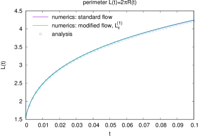
Figure 2. Evolution of modified flow (2.11)–(2.12): Perimeter of growing circle versus time: Analytic expression and results of standard and modified diffuse-interface flow (left). Analytic expression and results of modified diffuse-interface flow for the two variables $u$ and $v$ (right).

6.3.2. Benchmark: Example from [36]

In a second benchmark example we follow [33] and we compare in Fig. 3 a nearly stationary state in numerical results with analytic minimizers of the elastica functional found in [36]. Linnér and Jerome consider the elastica functional for graphs among all functions $f$ in $W^{2,2}((0,1))$ satisfying $f(0)=0$ and $f^{\prime}(1)=\infty$. Moreover, they prove existence and uniqueness and provide an explicit representation of the minimizer. For the numerical approach in this particular example, we have chosen a rectangular domain $\Omega=(-1.1,1.1)\times(2.2,2.2)$ and assume periodicity of all variables on $\partial\Omega$. For our simulations we choose initial conditions for $u$ and $v$ that represent an ellipse. In Fig. 3, one can see the nearly stationary level set $\{u_{h}=0.5\}$ at time $t\approx 0.2448$ compared to the analytic minimizer $\Gamma_{2}$ from [36]. Note that, similar to [33], we have shifted the solution from [36] in an appropriate way. Moreover, the discrete diffuse Willmore energies $\mathcal{W}_{\varepsilon}^{(1)}(u_{h})\approx 2.82307$ and $\mathcal{W}^{(2)}_{\varepsilon}(v_{h})\approx 2.88127$ are close to the analytic value $\approx 2.8711$. Together with the benchmark problem from Sec. 6.3.1 we can conclude that the modified flow (2.11),(2.12) yields a sound quantitative approximation of Willmore flow of curves.

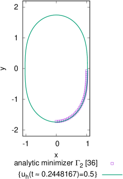
Figure 3. Almost stationary soultion of (2.11)–(2.12). Level curve $\{u_{h}=1/2\}$ at time $t\approx 0.2448$ and shifted version $\Gamma_{2}$ of the analytic minimizer from [36].

6.3.3. Colliding Circles

In Fig. 4, we consider an initial condition representing two circles. During the evolution of the modified flow the circles grow until the interfaces come sufficiently close, and unlike for the standard diffuse Willmore flow we do not observe any transversal intersections as reported in [33, 16]. In contrast, the interfaces stop moving at the meeting point and one can see the evolution of $u_{h}$ and $v_{h}$ towards almost stationary discrete states in Fig. 4.

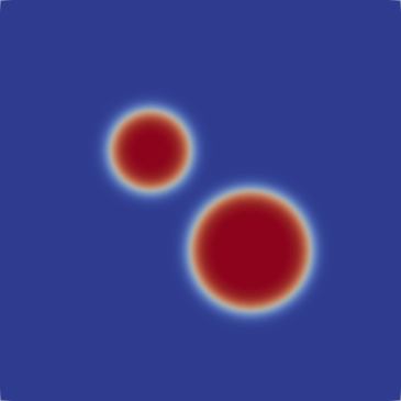
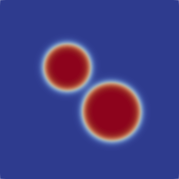
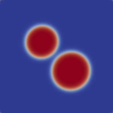
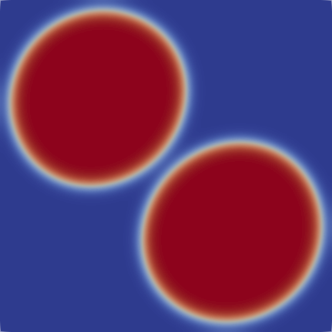
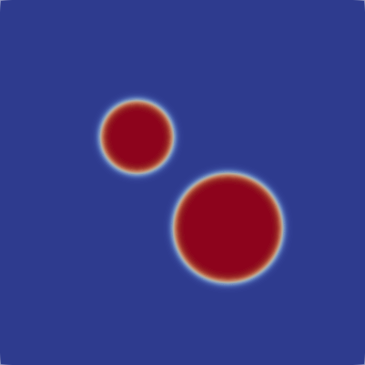
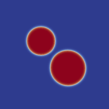
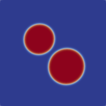
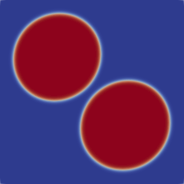
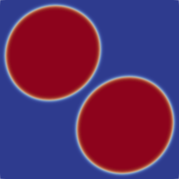
Figure 4. Evolution of modified flow (2.11)–(2.12): Discrete phase-fields $u_{h}$ and $v_{h}$ for different times $t=0$, $t\approx 0.0016$, $t\approx 0.0030$, $t\approx 0.0362$, $t\approx 0.1285$.

6.3.4. Adhesion to a domain inclusion

We come back to the motivating example from Fig. 1 and use the approach presented in this contribution in order to avoid transversal intersections which are undesired from the application point of view. From the modeling perspective, we follow [23] and consider a domain $\Omega\subset\mathbb{R}^{n}$ with a particle inclusion, which is given by an open set $\Omega_{p}\subset\joinrel\subset\Omega$. We introduce a sharp-interface membrane energy

(6.10) $$\mathcal{E}(\Gamma)\mathrel{\mathop{\mathchar 58\relax}}=\mathcal{W}(\Gamma)-\underbrace{w\int_{\Gamma_{\text{ad}}}\;\operatorname{d\!}\mathcal{H}^{n-1}(x)}_{=\mathrel{\mathop{\mathchar 58\relax}}\mathcal{E}_{\text{ad}}}$$

that includes an elastic contribution and an additional contact adhesion energy $\mathcal{E}_{\text{ad}}$. The latter measures the size of the contact set $\Gamma_{\text{ad}}\mathrel{\mathop{\mathchar 58\relax}}=\Gamma\cap\partial\Omega_{p}$, the adhesion strength is determined by the parameter $w\geq 0$. In addition, admissible membranes are confined to the set $\Omega\setminus\Omega_{p}$.

In order to obtain a diffuse-interface counterpart of (6.10), we introduce variables $\psi_{\varepsilon}^{(i)}\mathrel{\mathop{\mathchar 58\relax}}\Omega\to\mathbb{R}$, $i=1,2$,

(6.11) $$\psi^{(1)}_{\varepsilon}(x)\mathrel{\mathop{\mathchar 58\relax}}=q_{1}\Big{(}\frac{d_{p}}{\varepsilon}\Big{)},\quad\psi^{(2)}_{\varepsilon}(x)\mathrel{\mathop{\mathchar 58\relax}}=q_{2}\Big{(}\frac{d_{p}}{\varepsilon}\Big{)},\quad x\in\Omega,$$

with $d_{p}$ the signed distance to $\partial\Omega_{p}$, where $d_{p}>0$ in $\Omega_{p}$. The diffuse membrane energy then reads

(6.12) $$\mathcal{E}_{\varepsilon}(u,v)\mathrel{\mathop{\mathchar 58\relax}}=\mathcal{F}_{\varepsilon}(u,v)-\mathcal{E}^{(1)}_{\text{ad},\varepsilon}(u)-\mathcal{E}^{(2)}_{\text{ad},\varepsilon}(v)$$

with

$$\mathcal{E}^{(i)}_{\text{ad},\varepsilon}(u)\mathrel{\mathop{\mathchar 58\relax}}=\int_{\Omega}\left(\frac{\varepsilon}{2}|\nabla u|^{2}+\varepsilon^{-1}W_{i}(u)\right)2\varepsilon^{-1}W_{i}(\psi_{\varepsilon}^{(i)}),\quad i=1,2.$$

Moreover, in order to account for a volume constraint, we add a penalty energy to (6.12) penalizing deviations from a prescribed diffuse volume integral value. Finally, we include another penalty energy contribution

$$\sim\int_{\Omega}(\psi^{(1)}_{\varepsilon})^{2}(1-u-\psi_{\varepsilon}^{(1)})^{2}+\int_{\Omega}(\psi^{(2)}_{\varepsilon})^{2}(1-v-\psi_{\varepsilon}^{(2)})^{2}$$

which prevents the interface from going through the domain inclusion, where $\psi_{\varepsilon}\approx 1$. In Fig. 5 we see the results for the corresponding flow. For this particular example an adaptively refined grid has been applied, where the grid is locally refined or coarsened according to the values of $u_{h}$, $v_{h}$ and $\psi_{\varepsilon}$, see [5]. One observes that the formation of transversal interfaces as in Fig. 1 is now prevented by the new energy modification. For more detailed information, we refer to [45].

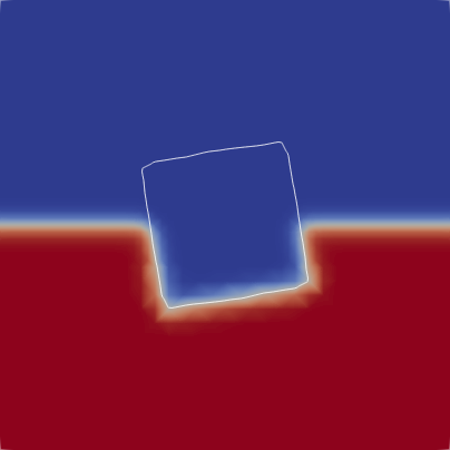
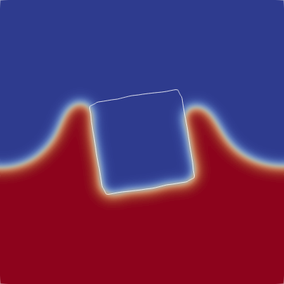
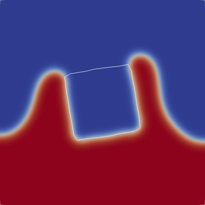
Figure 5. Evolution of modified flow for adhesion to domain inclusion application: Discrete phase-field $u_{h}$ for different times $t=0$, $t\approx 0.0011$, $t\approx 0.0340$, $t\approx 0.3678$.

6.3.5. Approximation of the lower-semicontinuous envelope of the elastica functional

Here we consider a particular set $E$ in the plane resembling a cloverleaf. The set has four connected components, each with a simple cusp. Due to the non-smooth boundary, the elastica functional is not defined for such a configuration. To associate an elastic energy to $E$ one can evaluate the value of the lower-semicontinuous envelope, given by

$$\overline{\mathcal{W}}(E)=\inf\{\liminf_{k\to\infty}\mathcal{W}(E_{k})\},$$

where the infimum is taken over all sequences $(E_{k})_{k}$ of sets $E_{k}\subset\joinrel\subset\Omega$ with $C^{2}$-boundary converging in an $L^{1}(\Omega)$ sense to $E$. The lower-semicontinuous envelope of the sum of area and elastica functional was studied in [7] and [8, 10], where also the cloverleaf example was considered. It was shown that for all configurations with an even number of simple cusps $\overline{\mathcal{W}}$ is finite. Moreover the minimization procedure in the definition of $\overline{\mathcal{W}}$ leads to an optimal system of curves that extends the boundary $\partial E$ by ‘ghost interfaces’ with even multiplicity. Here we consider a similar problem, where the minimization of the sum of length and elastica functional is replaced by the minimization of the elastica functional subject to a confinement constraint (to the computational domain $\Omega$). To obtain a diffuse approximation a modification of the classical approach is essential, since the latter in general leads to limit configurations with transversal intersections that carry an energy $\overline{\mathcal{W}}$ that is unbounded. We demonstrate here that our modified diffuse Willmore flow leads to reasonable results and configurations that correspond to an optimal system of curves arising in the minimization procedure associated to the definition of $\overline{\mathcal{W}}$ (even if we cannot provide a rigorous justification in the sense of convergence of our modified energy to the lower-semicontinuous envelope of the elastica functional).

With this aim let $E\subset\joinrel\subset\Omega$ be given by four symmetrically distributed drops described by so-called piriforms, see [35]. We introduce an additional energy contribution that penalizes deviation of the diffuse fields from the set $E$, given by

$$\mathcal{F}_{\psi_{\varepsilon}^{(1)}}(u)+\mathcal{F}_{\psi_{\varepsilon}^{(2)}}(v),\qquad\mathcal{F}_{\psi_{\varepsilon}^{(i)}}(u)=\frac{M_{\psi}^{\varepsilon}}{2}\int_{\Omega}(u-\psi_{\varepsilon}^{(i)})^{2},$$

where we choose

$$\psi_{\varepsilon}^{(i)}(x)\mathrel{\mathop{\mathchar 58\relax}}=q_{i}\left(\frac{d(x)}{\varepsilon}\right),\quad x\in\Omega,$$

where $d$ denotes the signed distance to $\partial E$, with $d>0$ in $E$. In Fig. 6, one can see a contour plot of $\psi^{(1)}_{\varepsilon,h}$ used for the simulation results in Fig. 7, where the evolution of $u_{h}$ for the standard flow with $\varepsilon=\frac{1}{16}$ towards an almost stationary state is shown. Starting from a circular interface one observes that the the discrete solutions $u_{h}$ approach the characteristic function of $E$. In the final (almost stationary) configuration the four cusps are connected by straight diffuse layers with transversal crossings. The computation of the discrete Willmore energy for the almost stationary state yields

(6.13) $$\mathcal{W}_{\frac{1}{16}}(u_{h})\approx 57.6219.$$

A numerical integration of the Willmore energy for the analytic parameterization of the four piriforms gives

(6.14) $$\mathcal{W}(\Gamma)\approx 64.5136.$$

The lower value of the approximate energy is due to the fact that for positive $\varepsilon>0$ an asymptotically small deviation of the diffuse phases from the cloverleaf is allowed. For smaller $\varepsilon$ values one obtains discrete diffuse-interface Willmore energies

$$\mathcal{W}_{\frac{1}{32}}(u_{h})\approx 61.7408\quad\text{and}\quad\mathcal{W}_{\frac{1}{64}}(u_{h})\approx 64.3346,$$

which shows the excellent approximation of the analytic value (6.14) for decreasing $\varepsilon$, see also plots of almost stationary solutions to the standard flow for $\varepsilon=\frac{1}{32}$ and $\varepsilon=\frac{1}{64}$ in Fig. 8.

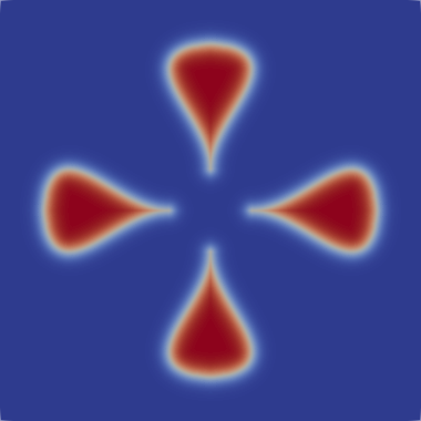
Figure 6. Contour plot of $\psi_{\varepsilon,h}^{(1)}$.

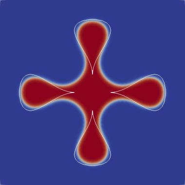
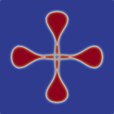
Figure 7. Evolution of standard flow ($\varepsilon=\frac{1}{16}$): Discrete phase-field $u_{h}$ for different times $t=0$, $t\approx 0.00020$, $t\approx 0.00485$, $t\approx 0.19485$.

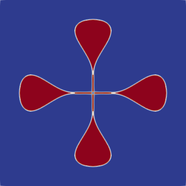
Figure 8. Almost stationary discrete solutions $u_{h}$ of standard flow ($\varepsilon=\frac{1}{32}$, left; $\varepsilon=\frac{1}{64}$, right).

The results for the corresponding simulation of the modified flow are displayed in Fig. 9. The method prohibits the formation of the transversal crossings observed for the standard flow. Instead, much thicker connections between the cusps are formed and this connections give a positive contribution to the Willmore energy. The discrete Willmore energy in this case becomes

(6.15) $$\mathcal{W}_{\frac{1}{16}}(v_{h})\approx 79.4029$$

substantially increased compared to (6.13). This is even more significant as the configuration still deviates from the set $E$ and hence takes more freedom to minimize the elastic energy.

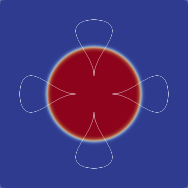
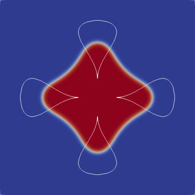
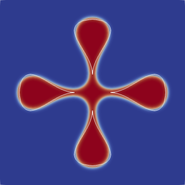
Figure 9. Evolution of modified flow ($\varepsilon=\frac{1}{8}$): Discrete phase-field $v_{h}$ for different times $t=0$, $t\approx 0.00019$, $t\approx 0.01096$, $t\approx 0.06896$.

For the modified flow with a two-component initial condition, one obtains in Fig. 10 an evolution towards an almost stationary state approximating the piriforms, where two components are connected by a quarter circle, see Fig. 11 for almost stationary states for approximations with reduced $\varepsilon$ values. The computation of the discrete Willmore energies then gives

(6.16) $$\mathcal{W}_{\frac{1}{16}}(v_{h})\approx 56.9323,\;\mathcal{W}_{\frac{1}{32}}(v_{h})\approx 64.2198,$$

$$\mathcal{W}_{\frac{1}{64}}(v_{h})\approx 68.8152,\;\mathcal{W}_{\frac{1}{128}}(v_{h})\approx 72.4494,\;\mathcal{W}_{\frac{1}{256}}(v_{h})\approx 74.9083,$$

and the analytic expression of the sharp-interface limit yields

$$\mathcal{W}(\Gamma)\approx 81.0483,$$

where one has to add the Willmore energy of four quarter circles to the energy of the piriforms in (6.14). The simulation of the standard flow with the same initial conditions as in Fig. 10 leads to results presented in Fig. 12. One observes an evolution with intermediate transversal crossings.

In conclusion we see that the minimization with the standard diffuse Willmore energy does not lead to configurations that attain the minimal energy with respect to the lower semi-continuous envelope. Instead, the cusps are connected with straight ghost interfaces that transversally intersect and have infinite energy $\overline{\mathcal{W}}$. In contrast, the modified energy leads to optimal configurations that are expected as the minimizing systems of curves in the characterization of $\overline{\mathcal{W}}$. In both cases, due to the presence of a large number of local minimizer, the stationary states of the corresponding gradient flows depend very much on the initial states. In order to find the minimal energy configurations sophisticated guesses are required.

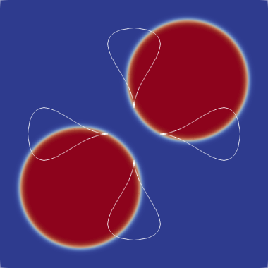
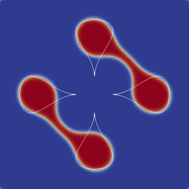
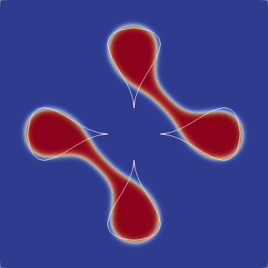
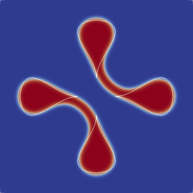
Figure 10. Evolution of modified flow ($\varepsilon=\frac{1}{8}$): Discrete phase-field $v_{h}$ for different times $t=0$, $t\approx 0.00102$, $t\approx 0.01002$, $t\approx 0.18402$.

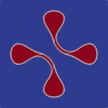
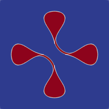
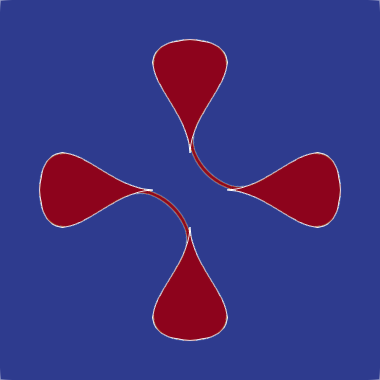
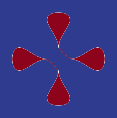
Figure 11. Almost stationary discrete solutions $v_{h}$ of modified flow for $\varepsilon=\frac{1}{16}$, $\varepsilon=\frac{1}{32}$, $\varepsilon=\frac{1}{64}$ and $\varepsilon=\frac{1}{128}$ (from left to right).

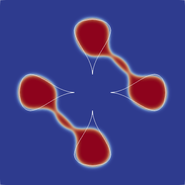
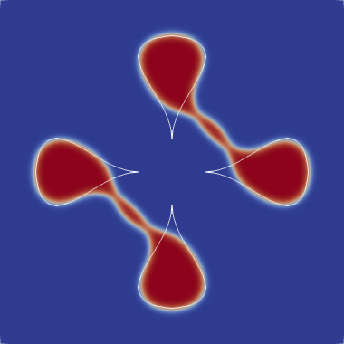
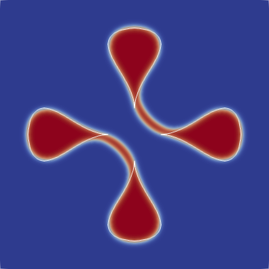
Figure 12. Evolution of standard flow ($\varepsilon=\frac{1}{16}$): Discrete phase-field $u_{h}$ for different times $t=0$, $t\approx 0.00011$, $t\approx 0.00159$, $t\approx 0.19510$.

References

- [1] Francesca Alessio, Alessandro Calamai and Piero Montecchiari “Saddle-type solutions for a class of semilinear elliptic equations.” In Adv. Differ. Equ. 12.4 Khayyam Publishing Company, Athens, OH, 2007, pp. 361–380
- [2] J.. Barrett, H. Garcke and R. Nürnberg “A parametric finite element method for fourth order geometric evolution equations” In J. Comput. Phys. 222.1, 2007, pp. 441–462 DOI: 10.1016/j.jcp.2006.07.026
- [3] J.. Barrett, H. Garcke and R. Nürnberg “Parametric approximation of Willmore flow and related geometric evolution equations” In SIAM J. Sci. Comput. 31.1, 2008, pp. 225–253 DOI: 10.1137/070700231
- [4] J.. Barrett, H. Garcke and R. Nürnberg “Numerical approximation of gradient flows for closed curves in ” In IMA J. Numer. Anal. 30.1, 2010, pp. 4–60 DOI: 10.1093/imanum/drp005
- [5] J.W. Barrett, R. Nürnberg and V. Styles “Finite element approximation of a phase field model for void electromigration” In SIAM J. Numer. Anal. 42.2, 2004, pp. 738–772 (electronic)
- [6] G. Bellettini “Variational approximation of functionals with curvatures and related properties” In J. Convex Anal. 4.1, 1997, pp. 91–108
- [7] G. Bellettini, G. Dal Maso and M. Paolini “Semicontinuity and relaxation properties of a curvature depending functional in D” In Ann. Scuola Norm. Sup. Pisa Cl. Sci. (4) 20.2, 1993, pp. 247–297
- [8] G. Bellettini and L. Mugnai “Characterization and representation of the lower semicontinuous envelope of the elastica functional” In Ann. Inst. H. Poincaré Anal. Non Linéaire 21.6, 2004, pp. 839–880
- [9] G. Bellettini and L. Mugnai “On the approximation of the elastica functional in radial symmetry” In Calc. Var. Partial Differential Equations 24.1, 2005, pp. 1–20
- [10] G. Bellettini and L. Mugnai “A varifolds representation of the relaxed elastica functional.” In J. Convex Anal. 14.3, 2007, pp. 543–564
- [11] G. Bellettini and M. Paolini “Some results on minimal barriers in the sense of De Giorgi applied to driven motion by mean curvature” In Rend. Accad. Naz. Sci. XL Mem. Mat. Appl. (5) 19, 1995, pp. 43–67
- [12] M. Beneš, K. Mikula, T. Oberhuber and D. Ševčovič “Comparison study for level set and direct Lagrangian methods for computing Willmore flow of closed planar curves” In Comput. Vis. Sci. 12.6, 2009, pp. 307–317 DOI: 10.1007/s00791-008-0112-2
- [13] T. Biben, K. Kassner and C. Misbah “Phase-field approach to three-dimensional vesicle dynamics” In Phys. Rev. E 72.4, Part 1, 2005
- [14] A. Bonito, R.. Nochetto and M.. Pauletti “Parametric FEM for geometric biomembranes” In J. Comput. Phys. 229.9, 2010, pp. 3171–3188 DOI: 10.1016/j.jcp.2009.12.036
- [15] Elie Bretin, François Dayrens and Simon Masnou “Volume reconstruction from slices” In SIAM J. Imaging Sci. 10.4, 2017, pp. 2326–2358 DOI: 10.1137/17M1116283
- [16] Elie Bretin, Simon Masnou and Édouard Oudet “Phase-field approximations of the Willmore functional and flow” In Numer. Math. 131.1, 2015, pp. 115–171 DOI: 10.1007/s00211-014-0683-4
- [17] Xavier Cabré and Joana Terra “Saddle-shaped solutions of bistable diffusion equations in all of .” In J. Eur. Math. Soc. (JEMS) 11.4 European Mathematical Society (EMS) Publishing House, Zurich, 2009, pp. 819–943
- [18] Luis Caffarelli, Nicola Garofalo and Fausto Segàla “A gradient bound for entire solutions of quasi-linear equations and its consequences” In Comm. Pure Appl. Math. 47.11, 1994, pp. 1457–1473 DOI: 10.1002/cpa.3160471103
- [19] F. Campelo and A. Hernandez-Machado “Dynamic model and stationary shapes of fluid vesicles” In European Physical Journal E 20.1, 2006, pp. 37–45
- [20] Anna Dall’Acqua, Chun-Chi Lin and Paola Pozzi “A gradient flow for open elastic curves with fixed length and clamped ends” In Ann. Sc. Norm. Super. Pisa Cl. Sci. (5) 17.3, 2017, pp. 1031–1066
- [21] Anna Dall’Acqua and Paola Pozzi “A Willmore-Helfrich -flow of curves with natural boundary conditions” In Comm. Anal. Geom. 22.4, 2014, pp. 617–669 DOI: 10.4310/CAG.2014.v22.n4.a2
- [22] Ha Dang, Paul C. Fife and L.. Peletier “Saddle solutions of the bistable diffusion equation” In Z. Angew. Math. Phys. 43.6, 1992, pp. 984–998 DOI: 10.1007/BF00916424
- [23] Sabyasachi Dasgupta, Thorsten Auth and Gerhard Gompper “Shape and orientation matter for the cellular uptake of nonspherical particles” In Nano letters 14.2 ACS Publications, 2014, pp. 687–693
- [24] Ennio De Giorgi “Some remarks on -convergence and least squares method” In Composite media and homogenization theory (Trieste, 1990) 5, Progr. Nonlinear Differential Equations Appl. Boston, MA: Birkhäuser Boston, 1991, pp. 135–142
- [25] K. Deckelnick, G. Dziuk and C.. Elliott “Computation of geometric partial differential equations and mean curvature flow” In Acta Numer. 14, 2005, pp. 139–232 DOI: 10.1017/S0962492904000224
- [26] Patrick W. Dondl, Antoine Lemenant and Stephan Wojtowytsch “Phase field models for thin elastic structures with topological constraint” In Arch. Ration. Mech. Anal. 223.2, 2017, pp. 693–736 DOI: 10.1007/s00205-016-1043-6
- [27] Patrick W. Dondl, Luca Mugnai and Matthias Röger “Confined Elastic Curves” In SIAM Journal on Applied Mathematics 71.6 SIAM, 2011, pp. 2205–2226 DOI: 10.1137/100805339
- [28] M. Droske and M. Rumpf “A level set formulation for Willmore flow” In Interfaces Free Bound. 6.3, 2004, pp. 361–378 DOI: 10.4171/IFB/105
- [29] Q. Du, C. Liu and X. Wang “A phase field approach in the numerical study of the elastic bending energy for vesicle membranes.” In J. Comput. Phys. 198.2, 2004, pp. 450–468
- [30] Q. Du, C. Liu and X. Wang “Simulating the deformation of vesicle membranes under elastic bending energy in three dimensions” In J. Comput. Phys. 212.2, 2006, pp. 757–777 DOI: 10.1016/j.jcp.2005.07.020
- [31] Gerhard Dziuk, Ernst Kuwert and Reiner Schätzle “Evolution of elastic curves in : existence and computation” In SIAM J. Math. Anal. 33.5, 2002, pp. 1228–1245 (electronic) DOI: 10.1137/S0036141001383709
- [32] C.. Elliott and B. Stinner “Modeling and computation of two phase geometric biomembranes using surface finite elements” In J. Comput. Phys. 229.18, 2010, pp. 6585–6612 DOI: 10.1016/j.jcp.2010.05.014
- [33] Selim Esedoḡlu, Andreas Rätz and Matthias Röger “Colliding interfaces in old and new diffuse-interface approximations of Willmore-flow” In Commun. Math. Sci. 12.1, 2014, pp. 125–147 DOI: 10.4310/CMS.2014.v12.n1.a6
- [34] Martina Franken, Martin Rumpf and Benedikt Wirth “A phase field based PDE constrained optimization approach to time discrete Willmore flow” In Int. J. Numer. Anal. Model. 10.1, 2013, pp. 116–138
- [35] J.D. Lawrence “A catalog of special plane curves”, Dover books on advanced mathematics Dover Publications, 1972 URL: https://books.google.de/books?id=F0DvAAAAMAAJ
- [36] Anders Linnér and Joseph W. Jerome “A unique graph of minimal elastic energy” In Trans. Amer. Math. Soc. 359.5, 2007, pp. 2021–2041 (electronic) DOI: 10.1090/S0002-9947-06-04315-7
- [37] P. Loreti and R. March “Propagation of fronts in a nonlinear fourth order equation.” In Eur. J. Appl. Math. 11.2, 2000, pp. 203–213
- [38] J. Lowengrub, A. Rätz and A. Voigt “Phase-field modeling of the dynamics of multicomponent vesicles: spinodal decomposition, coarsening, budding, and fission.” In Phys. Rev. E 79.3, 2009, pp. 0311926
- [39] L. Modica “The Gradient Theory of Phase Transitions and the Minimal Interface Criterion” In Arch. Rational Mech. Anal. 98, 1987, pp. 357–383
- [40] Luciano Modica “A gradient bound and a Liouville theorem for nonlinear Poisson equations” In Comm. Pure Appl. Math. 38.5, 1985, pp. 679–684 DOI: 10.1002/cpa.3160380515
- [41] Luciano Modica and Stefano Mortola “Un esempio di -convergenza” In Boll. Un. Mat. Ital. B (5) 14.1, 1977, pp. 285–299
- [42] Luciano Modica and Stefano Mortola “Some entire solutions in the plane of nonlinear Poisson equations” In Boll. Un. Mat. Ital. B (5) 17.2, 1980, pp. 614–622
- [43] Roger Moser “A higher order asymptotic problem related to phase transitions” In SIAM J. Math. Anal. 37.3, 2005, pp. 712–736 DOI: 10.1137/040616760
- [44] Luca Mugnai “Gamma-convergence results for phase-field approximations of the 2D-Euler elastica functional” In ESAIM Control Optim. Calc. Var. 19.3, 2013, pp. 740–753 DOI: 10.1051/cocv/2012031
- [45] A. Rätz and M. Röger “A diffuse-interface model accounting for elastic membrane energies with particle–membrane interaction” In preparation
- [46] Matthias Röger and Reiner Schätzle “On a modified conjecture of De Giorgi” In Math. Z. 254.4, 2006, pp. 675–714 DOI: 10.1007/s00209-006-0002-6
- [47] R.. Rusu “An algorithm for the elastic flow of surfaces” In Interfaces Free Bound. 7.3, 2005, pp. 229–239 DOI: 10.4171/IFB/122
- [48] S. Vey and A. Voigt “AMDiS: adaptive multidimensional simulations” In Computing and Visualization in Science 10.1, 2007, pp. 57–67
- [49] X. Wang “Asymptotic analysis of phase field formulations of bending elasticity models.” In SIAM J. Math. Anal. 39.5, 2008, pp. 1367–1401 DOI: 10.1137/060663519
- [50] X. Wang and Q. Du “Modelling and simulations of multi-component lipid membranes and open membranes via diffuse interface approaches” In J. Math. Biol. 56.3, 2008, pp. 347–371 DOI: 10.1007/s00285-007-0118-2
- [51] Xiaoqiang Wang, Lili Ju and Qiang Du “Efficient and stable exponential time differencing Runge-Kutta methods for phase field elastic bending energy models” In J. Comput. Phys. 316, 2016, pp. 21–38 DOI: 10.1016/j.jcp.2016.04.004
- [52] T.. Willmore “Riemannian geometry”, Oxford Science Publications New York: The Clarendon Press Oxford University Press, 1993, pp. xii+318
- [53] C. Zwilling “The diffuse interface approximation of the Willmore functional in configurations with interacting phase boundaries”, 2018 URL: http://dx.doi.org/10.17877/DE290R-19123