Study of long-term flux and photon Index distributions of blazars using RXTE observations

Abstract

We present a detailed study of flux and index distributions of three blazars (one FSRQ and two BL Lacs) by using 16 years of Rossi X-ray Timing Explorer archival data. The three blazars were chosen such that their flux and index distributions have sufficient number of data points ($\geq$90) with relatively less uncertainty ($\overline{\sigma_{err}^{2}}/\sigma^{2}$<0.2) in light curves. Anderson-Darling (AD) test and histogram fitting shows that flux distribution of FSRQ 3C273 is log-normal, while its photon index distribution is Gaussian. This result is consistent with linear Gaussian perturbation in the particle acceleration time-scale, which produces log-normal distribution in flux. However, for two BL Lacs viz. Mkn501 and Mkn421, AD test shows that their flux distributions are neither Gaussian nor log-normal, and their index distributions are non-normal. The histogram fitting of Mkn501 and Mkn421, suggests that their flux distributions are more likely to be a bi-modal, and their index distributions are double Gaussian. Since, Sinha et al. (2018) had shown that Gaussian distribution of index produces a log-normal distribution in flux, double Gaussian distribution of index in Mkn501 and Mkn421 indicates that their flux distributions are probably double log-normal. Observation of double log-normal flux distribution with double Gaussian distribution in index reaffirms two flux states hypothesis. Further, the difference observed in the flux distribution of FSRQ (3C273) and BL Lacs (Mkn501 and Mkn421) at X-rays, suggest that the low energy emitting electrons have a single log-normal flux distribution while the high energy ones have a double log-normal flux distribution.

1 Introduction

Blazars are the class of radio loud active galactic nuclei (AGNs), with relativistic jets oriented close to the observer’s line of sight (Urry & Padovani, 1995). The non-thermal emission from blazars extends from radio to $\gamma$-ray energies. Blazars are characterized by their extreme properties like luminous core, rapid variability, high polarization, superluminal motion, occasional spectacular flares etc. These extreme properties are usually attributed to the Doppler boosting of the emission which occurs from the relativistic regions in the jet. Blazars are broadly classified into two sub-classes, namely, BL Lac objects and Flat Spectrum Radio Quasars (FSRQs). The difference between these two sub-classes is based on the presence or absence of emission/absorption line features in their optical spectrum, such that FSRQs show strong emission lines whereas for BL Lacs, the emission lines are weak/absent (Urry & Padovani, 1995; Fan, 2003). The non-thermal emission originating from blazar jet produces a double humped spectral energy distribution (SED) (Fossati et al., 1998), with the low energy component peaking at optical/UV/soft X-ray energies, while the high energy component peaks at GeV energies. The low energy component is well established to be produced by synchrotron emission from relativistic electrons gyrating in the magnetic field of the jet, whereas the high energy component is usually attributed either to the inverse Compton (IC) scattering of low energy photons (Maraschi et al., 1992; Dermer et al., 1992; Shah et al., 2017) or to the hadronic cascades initiated in the jet (Böttcher, 2007). Based on the location of the peak frequency in the low energy component, blazars are further classified into three sub-classes namely, high energy peaked BL Lac (HBL; $\nu_{p}>10^{15.3}$ Hz; (Padovani & Giommi, 1995)), intermediate energy peaked BL Lac (IBL; $10^{14}<\nu_{p}{\leq}10^{15.3}$ Hz), and low energy peaked BL Lac (LBL; $\nu_{p}{\leq}10^{14}$ Hz) (Fan et al., 2016).

The light curves of blazars show unpredictable variations over a broad range of time-scales ranging from minutes to years across the entire electromagnetic spectrum. The clue to the mechanism causing such variations can be obtained by studying their long-term flux distributions. Typically, a Gaussian distribution of fluxes suggests additive processes, which is obtained when the flux variation is stochastic and linear. However, if the stochastic flux variation is non-linear, a Gaussian distribution in logarithmic flux values is expected, and such distributions are known as log-normal, which are often found in galactic and extra-galactic sources, like X-ray binaries, gamma-ray bursts, and AGNs (Uttley & McHardy, 2001; Negoro & Mineshige, 2002; Lyubarskii, 1997; Quilligan et al., 2002; Giebels & Degrange, 2009). In the case of AGNs, the log-normal behavior are observed on time-scales ranging from minutes to days (Gaskell, 2004); whereas, for X-ray binaries, such behavior is seen in sub-second time scales (Uttley et al., 2005). Among blazars, BL Lac is the first blazar in which log-normal distribution of X-ray flux was observed (Giebels & Degrange, 2009). Subsequently, such log-normal behavior in fluxes with the excess r.m.s correlating linearly with the average flux, have been found in different energy-bands for a HBL, PKS 2155-304 (H. E. S. S. Collaboration et al., 2017). Recently, a log-normal distribution of flux was shown in PKS 2155-304 at X-ray and optical bands by using ten years of data (Chevalier et al., 2019). In the very high energy (VHE) $\gamma$-ray band, the log-normal behavior of flux distribution has been detected in the well known high synchrotron peaked BL Lac objects Mrk 501 (Tluczykont et al., 2010; Romoli et al., 2018) and PKS 2155-304 (Aharonian et al., 2009; H.E.S.S. Collaboration et al., 2010). The brightest blazar sources seen by Fermi-LAT show a similar trend in their long term monthly binned $\gamma$-ray light curves (Shah et al., 2018). Also, using the Fermi-LAT observations, the long-term $\gamma$-ray flux variability of the VHE source 1ES 1011+496 is independently confirmed to be log-normal by Sinha et al., 2017. In addition to single log-normal distribution, the double log-normal profile has also been revealed at multi-wavelength bands for some blazars (Kushwaha et al., 2016a; Shah et al., 2018).

The log-normal behavior of these astrophysical sources is generally explained in terms of variations from the accretion disk, which are multiplicative in nature (Uttley et al., 2005; McHardy, 2010). However, the fluctuations in the accretion disk may not produce minute scale variability as seen in most of the blazar sources (Gaidos et al., 1996; Albert et al., 2007; Paliya et al., 2015). Therefore, as an alternative to the accretion disk model, the log-normal flux distribution in blazars have also been explained in terms of a sum of emission from a large collection of mini-jets, which are randomly oriented inside the relativistic jet (Biteau & Giebels, 2012). Moreover, recently it has been shown that a linear Gaussian perturbation in the particle acceleration time scale can produce the log-normal flux distribution (Sinha et al., 2018). They showed that perturbation in the acceleration time scale produces a Gaussian distribution in the index which in turn results in a log-normal distribution of the flux, whereas the perturbation in the particle cooling rate produces neither a Gaussian nor a Log-normal flux distribution.

In this work, we study the flux and photon index distribution properties of blazar sources having statistically significant light curves in the 16 years of RXTE observation. The sample selection criteria from the RXTE AGN catalog is described in Section $2, Characterization of flux/index distribution and correlation study between the flux and photon index is described in Section $3. The physical interpretations of the obtained flux distributions are discussed in Section $4.

2 RXTE archieve and Sample selection

The Rossi X-ray Timing Explorer (RXTE) public database provides the systematically analyzed long-term light curves and spectral information of AGN sources, for the period from January 1996 to January 2012. RXTE has two co-aligned instruments, the Proportional Counter Array (PCA; 2-60 keV) (Jahoda et al., 2006) and the High-Energy X-ray Timing Experiment (HEXTE; 15-250 keV) (Rothschild et al., 1998). It provides light curves in the energy range 2–10 keV. In these light curves, the sampling of data is uneven as different periods had been proposed for various scientific goals. However, despite the time gaps in the light curves, the sixteen years of RXTE observation provides a large data set, which are some times statistically suitable to investigate the variability behavior.

We first selected all the blazars from the RXTE AGN Timing & Spectral Database (RATSD ), for which the flux and photon spectral index light curves are available with more than 90 number of flux/index points. The spectra of these blazars in RATSD are mostly fitted with simple power-law model, except few BL Lac sources which are fitted better with a broken power-law model with break energy below $\approx$ 10 keV (Rivers et al., 2013). The RATSD provide light curves in the energy range 2-10 keV, 2-4 keV, 4-7 keV and 7-10 keV. However, in order to have flux light curves with good statistics, we consider flux light curves which have been obtained in the full energy range of 2–10 keV. Further, to select the light curves with good statistics, we define light curve significance fraction as

$$R=\frac{\overline{\sigma_{err}^{2}}}{\sigma^{2}}$$ (1)

where $\overline{\sigma_{err}^{2}}$ is the mean square error of flux/index distribution and $\sigma^{2}$ is the variance of flux/index distribution. From the selected blazars, only those sources are considered for further analysis which has $R<0.2$ in both the flux and index light curves. However, this condition was not satisfied in the unbinned index light curves (light curves taken directly from RATSD) of the blazars except Mkn 501, therefore, for each selected blazar, we binned the flux/index light curves by combining the flux/index points from 2 days to a maximum of 10 days. The upper limit of 10 days bin is chosen to ensure that the minimum number of flux/index points in the binned light curve is $\geq 90$. After implementing these conditions i.e., length of the light curve $\geq 90$ and $R<0.2$, we are restricted to two BL Lacs viz. Mkn 501, Mkn 421 and one FSRQ viz. 3C 273. The above conditions are met with 2-days time-bin in 3C 273 and 10-days time-bin for Mkn 421, while in Mkn 501, these conditions are satisfied in unbinned and two-days time binned light curves (see Table 1). However, in order to obtain evenly sampled light curves in all three sources, we have used two-days time binned light curve for Mkn 501. The length of light curves and the ‘R’ values of 3C 273, Mkn 501 and Mkn 421 are given in Table 1.
3C 273 is a well studied FSRQ source located at a redshift $z\sim 0.158$. The RXTE X-ray spectra of this source is fitted with a power-law model with an average power-law index of $\Gamma=$ 1.70$\pm$0.01 (Rivers et al., 2013). The obtained RXTE flux/index light curves of 3C 273 are shown in Fig. 1. The two BL Lac objects viz. Mkn 501 and Mkn 421 at a redshift of 0.033 and 0.031 respectively, are very well known high synchrotron peaked BL Lac (HBL) objects, with the low energy SED component peaking at frequency $\nu_{p}>10^{15.3}$ Hz. The RXTE spectra of these sources are fitted better with a broken power-law model (Rivers et al., 2013). For Mkn 501, the average values of power-law photon index before break energy ($\Gamma 1$) and after break energy ($\Gamma 2$) are obtained as 1.97$\pm$0.02 and 2.02$\pm$0.01 respectively with a break energy at 6.9$\pm$1.2 keV, where as for Mkn 421, the average values of $\Gamma 1$ and $\Gamma 2$ are obtained as 2.41$\pm$0.09 and 2.75$\pm$0.01 with break energy of 6.6$\pm$0.4 keV. The RXTE flux and $\Gamma 1$ light curves of Mkn 501 and Mkn 421 are shown in Figs 2 and 3.

Moreover, since RATSD provides light curves from a pointing instrument (PCA), there is a possibility of bias being introduced in the flux distributions, if the sources were preferentially observed in the high flux states. To check for this, we looked for correlation between the flux and time-gap (time between two observations) with the Spearman’s rank correlation test. The null hypothesis probability values (P-value) for 3C273, Mkn 501 and Mkn 421 are obtained as 0.07, 0.15 and 0.08 respectively. In the case of Spearman’s correlation, the null hypothesis ($H_{0}$) is that there is no correlation between two variables, and we reject the null hypothesis if P<0.01. Therefore, the obtained P-values indicate that there is no significant correlation between flux and time-gap.

Table 1: Light curve significance fraction R values for the unbinned/binned flux and index light curves. Col:-  1: Selected blazars satisfying the conditions R<0.2 and length of binned flux/index light curve $\geq 90$, 2: Number of data points in the distributions, 3: R-value for index light curve, and 4: R-value for the flux light curve.

Blazar name	Number of	$R_{\Gamma}$	$R_{Flux}$
	data points
3C 273	1960 (unbinned)	0.22	$2.0\times 10^{-3}$
	1151 (2-days binned)	0.19	$1.5\times 10^{-3}$
Mkn 501	496 (unbinned)	0.05	$1.0\times 10^{-4}$
	188 (2-days binned)	0.06	$1.0\times 10^{-4}$
Mkn 421	1182 (unbinned)	0.75	$6.8\times 10^{-5}$
	93 (10-days binned)	0.17	$9.6\times 10^{-6}$

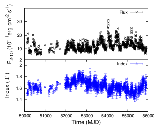
Figure 1: The X-ray flux/index light curves of 3C 273 obtained by using the sixteen years of RXTE archive data. Top panel: 2-days time binned flux light curve obtained in the energy range 2-10 keV, bottom panel: 2-days time binned index light curve.

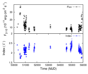
Figure 2: The X-ray flux and $\Gamma 1$ light curves of Mkn 501 obtained by using the sixteen years of RXTE archive data. Top panel and bottom panel are the same as in Fig. 1.

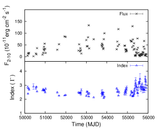
Figure 3: The X-ray flux and $\Gamma 1$ light curves of Mkn 421 obtained by using the sixteen years of RXTE archive data. Top panel: 10-days time binned flux light curve obtained in the energy range 2-10 keV, bottom panel: 10-days time binned $\Gamma 1$ light curve.

3 Distribution study for blazars

3.1 AD test

Generally, the flux distribution of blazar light curves shows an asymmetric/tailed trend. Anderson-Darling (AD) test statistic is an useful tool for the normality test, which is sensitive towards the tails of a distribution (Press et al., 1992). The null hypothesis ($H_{0}$) of the AD test is that the data sample is drawn from a particular distribution (say normal distribution in our case). The AD test calculates the null hypothesis probability value (p–value) such that p–value < 0.01 would indicate the deviation from the normality of the sample.

The AD test for 3C 273 shows that the p–values for flux in log-scale and index in normal-scale are larger than 0.01, which suggests the flux distribution is consistent with a log-normal and the index distribution with a normal one. However, for the two BL Lac objects viz. Mkn 501 and Mkn 421, p–values for flux in linear-scale and log-scale are much smaller than 0.01, which indicates that the flux distribution will be neither normal nor log-normal. Moreover, the p–value of index distribution also suggests a non-normal distribution of index in Mkn 501 and Mkn 421. The AD test results of 3C 273, Mkn 501 and Mkn 421 are summarized in Table 2.

3.2 Histogram of Flux and Index

Histogram fitting is also a helpful tool to characterize the nature of the distribution. Here, we construct the normalized histograms of the logarithm of flux and photon index in linear-scale for the three selected blazars. The bin-widths of the histogram are chosen such that each bin carries an equal number of data points. In the case of FSRQ 3C 273, the single peak in the flux and index histograms suggest for the single distribution; hence we fitted these histograms with the probability density function (PDF) given by

$$\rm f(x)=\frac{1}{\sqrt{2\pi\sigma^{2}}}e^{\frac{-(x-\mu)^{2}}{2\sigma^{2}}}$$ (2)

where $\rm\mu$ and $\rm\sigma$ are the centroid and width of the distribution. The flux and index histograms along with best fitted PDF (equation 2) are shown in the multiplot (Fig. 4) and the best fit parameters are summarized in Table 3. The fit parameters confirm that the flux distribution of 3C 273 is log-normal while its index is normally distributed. These results are consistent with the results obtained from the AD test statistic. On the other hand, the flux and index histograms of the two BL Lacs (Mkn 501 and Mkn 421) show a double-peaked structure. Also, the AD test results of these two BL Lacs show that the flux distribution is neither Gaussian nor log-normal, and the index distribution is not Gaussian. We therefore analyzed these distributions by fitting their histograms with double PDF

$$\rm d(x)=\frac{a}{\sqrt{2\pi\sigma_{1}^{2}}}e^{\frac{-(x-\mu_{1})^{2}}{2\sigma_{1}^{2}}}\ +\frac{(1-a)}{\sqrt{2\pi\sigma_{2}^{2}}}e^{\frac{-(x-\mu_{2})^{2}}{2\sigma_{2}^{2}}}$$ (3)

where, $\rm a$ is the normalization fraction, $\rm\mu_{1}$ and $\rm\mu_{2}$ are the centroids of the distribution with widths $\rm\sigma_{1}$ and $\rm\sigma_{2}$, respectively. The fit of flux histogram in log-scale and index histogram in linear-scale with equation 3 will result in the double log-normal fit of the flux distribution and double normal fit of the index distribution. During the double log-normal fit of flux histogram, we have kept all parameters free viz. $\mu_{1}$, $\mu_{2}$, $\sigma_{1}$, $\sigma_{2}$ and a. However, in case of double normal fit of index histogram, we have fixed the normalization fraction ‘a’ to the best fit parameter value obtained in the double log-normal flux histogram fit and carried fitting with free parameters as $\mu_{1}$, $\mu_{2}$, $\sigma_{1}$ and $\sigma_{2}$. The same normalization fraction in the flux and index double PDF will ensure the similar contribution of the respective components in the flux and index distribution. The best fit parameter values of fitting the double distribution flux/index histograms with equation 3 are given in Table 4 and corresponding plots are shown in Figs 5 and 6. In case of Mkn 421, the error on the normalization fraction ‘a’ is not well constrained due to poor data statistics in the flux histogram, its best fit value ranges from 0.05–0.95. In this case, we have fixed the normalization fraction ‘a’ for both flux and index distribution as 0.3 (Table 4). The double log-normal fit to flux histograms of Mkn 501 and Mkn 421 gave a ${\chi^{2}}/{dof}$ of ${38.28}/{33}$ and ${11.85}/{15}$ respectively, while the other double distribution functions, such as combination of log-normal and Gaussian gave a ${\chi^{2}}/{dof}$ of ${38.38}/{33}$ for Mkn 501 and ${12.75}/{15}$ for Mkn 421. Combination of Gaussian and log-normal gave a ${\chi^{2}}/{dof}$ of ${50.36}/{33}$ for Mkn 501 and ${14.10}/{15}$ for Mkn 421, while a double Gaussian fit gave a ${\chi^{2}}/{dof}$ of ${41.58}/{33}$ for Mkn 501 and ${14.70}/{15}$ for Mkn 421. These reduced $\chi^{2}$ values suggest that the double log-normal fit and lognormal+Gaussian fit to the flux histograms of two BL Lacs are equally good. The best fit parameter values obtained by fitting the flux histogram with lognormal+Gaussian PDF are given in Table 5. Further, we found that the photon index distribution in both Mkn 501 and Mkn 421 are fitted with the double Gaussian distribution function with ${\chi^{2}}/{dof}$ of ${39.1}/{34}$ and $16.94/14$ respectively.

Table 2: AD test results for the flux/index distribution of three selected blazars viz. 3C 273, Mkn 501 and Mkn 421 Col:- 1: Selected blazars satisfying the conditions R<0.2 and length of binned flux/index light curve $\geq 90$, 2: Number of data points in the distributions, 3,4: AD statistics for Flux and Logarithm of flux distribution, and 5: AD statistics for index distribution.

Blazar name	Number of	Normal (Flux)	Log-normal (Flux)	Normal (Spectral index)
	data points	AD(p–value)	AD(p–value)	AD(p–value)
3C 273	1151 (2-days binned)	13.02 (<$2.2\times 10^{-16}$)	0.76 (0.06)	0.57 (0.14)
Mkn 501	188 (2-days binned)	15.89 (<$2.2\times 10^{-16}$)	2.78 ($4.96\times 10^{-7}$)	1.24 ($3.0\times 10^{-3}$)
Mkn 421	93 (10-days binned)	2.29 ($7.44\times 10^{-6}$)	1.27 ($2.5\times 10^{-3}$)	1.09 ($7.0\times 10^{-3}$)

Table 3: Best fit parameter values of the PDF (equation 2) fitted to the logarithm of flux and index histograms. Col:- 2: Histogram obtained from the logarithm of flux and linear index distribution, 3,4: Best fit values of $\mu$ and $\sigma$, 5: Degrees of freedom and 6: Reduced $\chi^{2}$.

Blazar name	Histogram	$\mu$	$\sigma$	dof	$\rm\chi^{2}/dof$
3C 273	log10(Flux)	-9.922$\pm$0.004	0.124$\pm$0.003	21	0.92
	Index	1.642$\pm$0.003	0.088$\pm$0.002	21	1.22

Table 4: Best fit parameter values of the double PDF (equation 3) fitted to the logarithm of flux and index histograms. Col:- 2: Histogram obtained from the logarithm of flux and linear index distribution, 3–6: Best fit values of $\mu_{1}$, $\sigma_{1}$, $\mu_{2}$ and $\sigma_{2}$, 7: Normalization fraction, 8: Degrees of freedom and 9: Reduced $\chi^{2}$.

Blazar name	Histogram	$\mu_{1}$	$\sigma_{1}$	$\mu_{2}$	$\sigma_{2}$	a	dof	$\rm\chi^{2}/dof$
Mkn 501	log10(Flux)	-9.62$\pm$0.04	0.10$\pm$0.03	-10.02$\pm$0.02	0.14$\pm$0.02	0.83$\pm$0.06	33	1.16
	Index	1.74$\pm$0.03	0.09$\pm$0.02	2.19$\pm$0.02	0.15$\pm$0.01	0.83	34	1.15
Mkn 421	log10(Flux)	-9.36$\pm$0.05	0.26$\pm$0.05	-10.10$\pm$0.08	0.29$\pm$0.08	0.3	15	0.79
	Index	2.54$\pm$0.05	0.21$\pm$0.04	3.09$\pm$0.48	0.51$\pm$0.31	0.3	14	1.21

Table 5: Best fit parameter values of the double PDF (lognormal+Gaussian) fitted to the logarithm of flux histogram. Col:- 2: Histogram obtained from the logarithm of flux distribution, 3–6: Best fit values of $\mu_{1}$, $\sigma_{1}$, $\mu_{2}$ and $\sigma_{2}$, 7: Normalization fraction, 8: Degrees of freedom and 9: Reduced $\chi^{2}$.

Blazar name	Histogram	$\mu_{1}$	$\sigma_{1}$	$\mu_{2}$	$\sigma_{2}$	a	dof	$\rm\chi^{2}/dof$
Mkn 501	log10(Flux)	-10.03$\pm$0.03	0.14$\pm$0.02	2.26e-10$\pm$3.998e-11	6.51e-11$\pm$2.10e-11	0.79$\pm$0.09	33	1.163
Mkn 421	log10(Flux)	-10.10$\pm$0.08	0.28$\pm$0.08	4.07e-10$\pm$5.20e-11	2.48e-10$\pm$4.43e-11	0.3	15	0.85

3.3 Correlation study

The three blazars selected from RXTE catalog has a sufficient number of data points to study the correlation between the photon index and the flux in the 2-10 keV energy band. We have used the Spearman’s rank correlation method to assess the correlation behavior between the index and flux. The obtained Spearman’s rank correlation coefficient ($r_{s}$), its chance correlation probability (P) and the correlation slope (A) are summarized in Table 6. The correlation parameters show a significant negative correlation between the flux and index in all the three blazars, which is the usual trend blazars show across the electromagnetic spectrum (Wierzcholska et al., 2015; Pandey et al., 2017; Brown & Adams, 2011). In the correlation plots (left top panel in Figs 4, 5 and 6), gray bands represent the 1-$\sigma$ error on the centroids of the logarithm of flux and index distributions (Figs 4, 5 and 6). In the bottom panel of Fig. 6, the error on higher index centroid is large, so a single vertical line is shown instead of a gray band.

Table 6: Spearman Correlation results obtained by comparing flux and index distribution of three selected blazars. Col:- 1: Selected blazar sources 2: Spearman’s rank correlation coefficient $(r_{s})$, 3: Probability chances for correlation (P) and 4: Slope of the best fitted line to correlation plots (A).

Blazar name	$r_{s}$	P	A
3C 273	-0.60	$2.0\times 10^{-4}$	-0.61$\pm$0.22
Mkn 501	-0.65	$2.96\times 10^{-24}$	-0.94$\pm$0.06
Mkn 421	-0.86	$7.25\times 10^{-29}$	-1.21$\pm$0.07

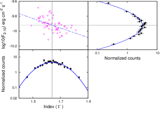
Figure 4: Multi-plot for the characterization of flux/index distribution of 3C 273. Top panel left is the logarithm of flux vs index scatter plot along with the best fit line (dotted line). Top panel right is the histogram of logarithmic of flux distribution. Bottom panel is the histogram of index distribution. The solid curve in the top panel right and bottom panel indicates the best fitted PDF (equation 2). The vertical and horizontal gray bands indicate the 1-$\sigma$ error range on the centroid ($\mu$) of the PDF (equation 2) fitted to the index distribution and logarithm of flux distribution respectively.

.

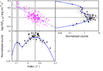
Figure 5: Multi-plot for the characterization of flux/index distribution of Mkn 501. Top panel left is the logarithm of flux vs index scatter plot along with the best fit line (dotted line). Top panel right is the histogram of logarithm of flux distribution. Bottom panel is the histogram of index distribution. The solid curve in the top panel right and bottom panel indicates the best fitted double PDF (equation 3). The vertical and horizontal gray bands indicate the 1-$\sigma$ error range on the centroids ($\mu 1$, $\mu 2$) of the double PDF (equation 3) fitted to the index distribution and logarithm of flux distribution respectively.

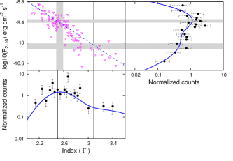
Figure 6: Multi-plot for the characterization of flux/index distribution of Mkn 421. The three panels in this plot are same as described in Fig. 5. A single vertical line represents the centroid value of the higher index distribution (Section 3.3).

4 Discussion

After selecting three blazars viz. 3C 273, Mkn 501 and Mkn 421 from the sample of blazars in the RXTE catalog, we used the AD test and histogram fitting to characterize their flux and index distributions. We found that the flux distribution of FSRQ 3C 273 follows a log-normal distribution while its index is Gaussian distributed. The log-normal distribution of flux in 3C 273 is also observed in the monthly binned $\gamma$-ray light curve (Shah et al., 2018). Since the variations in the index are related to the fluctuations in acceleration and escape time scales of the emitting particles in the acceleration region, the observed Gaussian distribution in index therefore indicate a linear normal fluctuations in the intrinsic time scales in the acceleration region. This result is consistent with the study by Sinha et al., 2018, where they showed that the linear normal fluctuation in the intrinsic particle acceleration time scale in the acceleration region can produce a log-normal flux distribution. The connection of log-normal flux distribution with the Gaussian index variation indicates that the source of X-ray flux variation in 3C 273 are not from the accretion disc, instead, the perturbations are mostly local to the jet.

Using the AD test, we found that the flux and index distributions of two BL Lacs viz. Mkn 501 and Mkn 421 are not consistent with a single distribution, and their histograms can be fitted with a double distribution. Interestingly, the overlapping of the centroids (within 1-$\sigma$ error – gray bands in Figs 5 and 6) of the double distributions in the log of flux and index distribution on the best fitted correlation line (blue dotted line in the correlation plots), with same normalization fraction values for both the distributions (Section 3.3, Table 4), implies that the double distribution in photon index is connected to the double distribution in flux. The reduced $\chi^{2}$ test shows that the flux distributions of Mkn 501 and Mkn 421 are either double log-normal or combination of log-normal and Gaussian, while their index distributions are double Gaussian. However, using the interpretation of Sinha et al., 2018, the double Gaussian distribution in the index would preferably indicate double log-normal distribution in flux. Sinha et al., 2018, showed that Gaussian distribution in the index can be initiated through linear fluctuations in the particle acceleration rate and hence, the log-normal flux distribution may carry information regarding the acceleration processes in the blazar jets.

In the study of multi-wavelength flux variations in PKS 1510-089, the two distinct log-normal profiles found in the flux distribution at near-infrared (NIR), optical and $\gamma$-ray energies are connected to two possible flux states in the source (Kushwaha et al., 2016b). In our work, the observation of double Gaussian distribution in index with bi-lognormal flux distribution in Mkn 501 and Mkn 421 further confirms the two flux states hypothesis. Moreover, contrary to double log-normal flux distribution in Mkn 501 and Mkn 421 in X-ray, the study of the $\gamma$-ray flux distribution of brightest Fermi blazars show a single log-normal flux distribution at $\gamma$-ray energy (Shah et al., 2018). However, it should be noted that the results of Shah et al. (2018) are obtained from light curves with a bin size of a month, which is longer than those used in this work. A longer binning might remove the second component of the distribution. In case of HBL sources like Mkn 501 and Mkn 421, the X-ray spectrum lies beyond the synchrotron peak and hence is mainly emitted by the high-energy end of the electron distribution. While in FSRQs, the X-ray emission is mainly due to the low energy tail of the electron distribution. Further, in the case of HBL sources, the low energy $\gamma$-ray spectrum occurs before the break energy of the inverse Compton component. Therefore, the differences observed in the flux distribution of FSRQ 3C 273 and HBL’s (Mkn 501 and Mkn 421) at X-rays may possibly be related to the energy of emitting particles. Thus, it seems that low energy emitting particles produce a single log-normal flux distribution while the high energy tail of the electron distribution produces double log-normal flux distribution. However, such inference can be confirmed by carrying out a detailed flux distribution study for a sample of sources with more statistically significant light curves. In this direction, a systematic regular long-term monitoring of blazars with MAXI would be important to probe such information. It will be interesting and important to quantify the flux distribution of these sources in other wave-bands, as that may strengthen the results presented here. However, continuous significant and reliable detection of flux and index at other bands is not available at present. We note that the upcoming Cherenkov Telescope Array (CTA Consortium & Ong, 2019) may provide such high quality light curves in gamma-rays.

References

- Aharonian et al. (2009) Aharonian F., et al., 2009, A&A, 502, 749
- Albert et al. (2007) Albert J., et al., 2007, ApJ, 669, 862
- Biteau & Giebels (2012) Biteau J., Giebels B., 2012, A&A, 548, A123
- Böttcher (2007) Böttcher M., 2007, Ap&SS, 307, 69
- Brown & Adams (2011) Brown A. M., Adams J., 2011, MNRAS, 413, 2785
- CTA Consortium & Ong (2019) CTA Consortium Ong R. A., 2019, in European Physical Journal Web of Conferences. p. 01038 (arXiv:1904.12196), doi:10.1051/epjconf/201920901038
- Chevalier et al. (2019) Chevalier J., Sanchez D. A., Serpico P. D., Lenain J.-P., Maurin G., 2019, MNRAS, 484, 749
- Dermer et al. (1992) Dermer C. D., Schlickeiser R., Mastichiadis A., 1992, A&A, 256, L27
- Fan (2003) Fan J. H., 2003, ApJ, 585, L23
- Fan et al. (2016) Fan J. H., et al., 2016, ApJS, 226, 20
- Fossati et al. (1998) Fossati G., Maraschi L., Celotti A., Comastri A., Ghisellini G., 1998, MNRAS, 299, 433
- Gaidos et al. (1996) Gaidos J. A., et al., 1996, Nature, 383, 319
- Gaskell (2004) Gaskell C. M., 2004, ApJ, 612, L21
- Giebels & Degrange (2009) Giebels B., Degrange B., 2009, A&A, 503, 797
- H. E. S. S. Collaboration et al. (2017) H. E. S. S. Collaboration et al., 2017, A&A, 598, A39
- H.E.S.S. Collaboration et al. (2010) H.E.S.S. Collaboration et al., 2010, A&A, 520, A83
- Jahoda et al. (2006) Jahoda K., Markwardt C. B., Radeva Y., Rots A. H., Stark M. J., Swank J. H., Strohmayer T. E., Zhang W., 2006, ApJS, 163, 401
- Kushwaha et al. (2016a) Kushwaha P., Chandra S., Misra R., Sahayanathan S., Singh K. P., Baliyan K. S., 2016a, ApJ, 822, L13
- Kushwaha et al. (2016b) Kushwaha P., Chandra S., Misra R., Sahayanathan S., Singh K. P., Baliyan K. S., 2016b, ApJ, 822, L13
- Lyubarskii (1997) Lyubarskii Y. E., 1997, MNRAS, 292, 679
- Maraschi et al. (1992) Maraschi L., Ghisellini G., Celotti A., 1992, ApJ, 397, L5
- McHardy (2010) McHardy I., 2010, in Belloni T., ed., Lecture Notes in Physics, Berlin Springer Verlag Vol. 794, Lecture Notes in Physics, Berlin Springer Verlag. p. 203, doi:10.1007/978-3-540-76937-8_8
- Negoro & Mineshige (2002) Negoro H., Mineshige S., 2002, PASJ, 54, L69
- Padovani & Giommi (1995) Padovani P., Giommi P., 1995, ApJ, 444, 567
- Paliya et al. (2015) Paliya V. S., Böttcher M., Diltz C., Stalin C. S., Sahayanathan S., Ravikumar C. D., 2015, ApJ, 811, 143
- Pandey et al. (2017) Pandey A., Gupta A. C., Wiita P. J., 2017, ApJ, 841, 123
- Press et al. (1992) Press W. H., Teukolsky S. A., Vetterling W. T., Flannery B. P., 1992, Numerical recipes in FORTRAN. The art of scientific computing, Cambridge Univ. Press, Cambridge
- Quilligan et al. (2002) Quilligan F., McBreen B., Hanlon L., McBreen S., Hurley K. J., Watson D., 2002, A&A, 385, 377
- Rivers et al. (2013) Rivers E., Markowitz A., Rothschild R., 2013, ApJ, 772, 114
- Romoli et al. (2018) Romoli C., Chakraborty N., Dorner D., Taylor A., Blank M., 2018, Galaxies, 6, 135
- Rothschild et al. (1998) Rothschild R. E., et al., 1998, ApJ, 496, 538
- Shah et al. (2017) Shah Z., Sahayanathan S., Mankuzhiyil N., Kushwaha P., Misra R., Iqbal N., 2017, MNRAS, 470, 3283
- Shah et al. (2018) Shah Z., Mankuzhiyil N., Sinha A., Misra R., Sahayanathan S., Iqbal N., 2018, Research in Astronomy and Astrophysics, 18, 141
- Sinha et al. (2017) Sinha A., Sahayanathan S., Acharya B. S., Anupama G. C., Chitnis V. R., Singh B. B., 2017, ApJ, 836, 83
- Sinha et al. (2018) Sinha A., Khatoon R., Misra R., Sahayanathan S., Mandal S., Gogoi R., Bhatt N., 2018, MNRAS, 480, L116
- Tluczykont et al. (2010) Tluczykont M., Bernardini E., Satalecka K., Clavero R., Shayduk M., Kalekin O., 2010, A&A, 524, A48
- Urry & Padovani (1995) Urry C. M., Padovani P., 1995, PASP, 107, 803
- Uttley & McHardy (2001) Uttley P., McHardy I. M., 2001, MNRAS, 323, L26
- Uttley et al. (2005) Uttley P., McHardy I. M., Vaughan S., 2005, MNRAS, 359, 345
- Wierzcholska et al. (2015) Wierzcholska A., Ostrowski M., Stawarz Ł., Wagner S., Hauser M., 2015, A&A, 573, A69