Stability of Non-Linear Filter for Deterministic Dynamics

Abstract.

This papers shows that nonlinear filter in the case of deterministic dynamics is stable with respect to the initial conditions under the conditions that observations are sufficiently rich, both in the context of continuous and discrete time filters. Earlier works on the stability of the nonlinear filters are in the context of stochastic dynamics and assume conditions like compact state space or time independent observation model, whereas we prove filter stability for deterministic dynamics with more general assumptions on the state space and observation process. We give several examples of systems that satisfy these assumptions. We also show that the asymptotic structure of the filtering distribution is related to the dynamical properties of the signal.

1. Introduction

The Bayesian formulation of the data assimilation problem [2, 28, 38, 3, 14] quite naturally leads to the problem of non-linear filtering, which had its roots in engineering applications and for which a rigorous foundational theory had been established in later half of twentieth century [45, 6, 24]. Filtering aims at estimating state of a system at a particular instant given some noisy observations of the system up to that instant. More precisely, we want to study the evolution of conditional distribution, referred to as filter or optimal filter from now on, of the state of the system at time $t$ given the $\sigma$-algebra generated by the observations made up to $t$, where the time $t$ is allowed to be either discrete or continuous. The evolution equation of the conditional distribution takes as inputs the observation path which drives the equation and the initial condition of the system, i.e., the probability distribution at the initial time.

In continuous time, this evolution equation is given by Kushner-Stratanovich (KS) equation whose solution is a measure valued process (conditional distribution in this case) and initial condition of KS equation is the probability distribution of initial condition of the system. In many situations, this initial condition is unknown and hence, it is desirable to know whether the non-linear filter is sensitive to the initial condition, at least for large times. In other words, we desire for solution to KS equation to be asymptotically stable with respect to the initial condition in case of continuous time. The notion of filter stability is analogously defined in the case of discrete time setting. This property of the filter is referred to as filter stability [45, 40]. Essentially, for stable filters, observations will correct for the mistake of wrongly initialising the filter, as more and more observations are made.

In the context of data assimilation in the earth sciences, the signal or the system being observed is the ocean and/or the atmosphere. Some of the important characteristics of these systems are that: (i) they are high dimensional; (ii) the observations are sparse and noisy; (iii) the dynamical models are very commonly deterministic [36],[3, Section 1.5], and (iv) these systems are chaotic. Thus many numerical algorithms that focus on one or more of these characteristics are being developed, though only a few theoretical results related to filtering for deterministic, chaotic signal dynamics have been established so far. This paper provide filter stability results precisely for such systems.

1.1. A summary of previous results

The problem of filter stability has been studied by many authors under different conditions on the system and observations. Stability of the filter in case of Kalman-Bucy filter is studied in [35, 9] under the conditions of uniform controllability and uniform observability and in case of Beneš filters is studied in [34]. Exponential stability of the filter has been established in the case of continuous time, ergodic signal and non-compact domain in [4] and in the case of discrete time, non-ergodic signal and non-compact domain in [13]. In [5, 12], filter stability is achieved using the Hilbert projective metric and Birkhoff’s contraction inequality. The filter stability in the case when signal is a general Markov process with a unique invariant measure under suitable regularity conditions is studied in [11]. In [19] it is proved, using relative entropy arguments, that some appropriate distance of correctly initialised and incorrectly initialised conditional distribution of specific functions of state (namely observation function) goes to zero. Moreover, they show that the relative entropy of optimal filter with respect to incorrectly initialised filter is a non-negative supermartingale. We refer the reader to [18, 40, 17] and the references therein, for more details regarding tools involved and results in the filter stability.

In general, proving filter stability requires ergodicity of the signal or making sufficiently rich enough observations, the precise form of the latter condition being observability. Roughly speaking, filtering model is said to be observable when two observation paths (initialised with two initial conditions) have same distribution and it implies that initial conditions are identically distributed. Using this notion, filter stability is established in [42] in discrete time and in [41] in continuous time. In [32], the authors used a more general version of observability to establish filter stability in discrete time. Note that in all the works mentioned in this section, the signal is a stochastic dynamical system.

1.2. Main contributions

In this paper, we prove in Theorem 3.8 the stability of a general nonlinear filter with deterministic signal dynamics in continuous time (and an analogous Theorem 4.10 in discrete time). Previous results of stability with linear deterministic dynamics and linear observations can be found in [23, 10] in the case of discrete time and in [33, 37] in the case of continuous time. The problem of accuracy (which is a measure of deviation of the filter from the signal) of the filter for deterministic dynamics is studied in [16], and we rely heavily on the techniques used in that study. In particular, the stability result in Theorem 3.8 is obtained by first proving, in Theorem 3.1 (and analogous Theorem 4.8 in discrete time), the consistency of the smoother, i.e., the asymptotic convergence of the conditional distribution of the initial condition given the observations (which is a particular case of the smoothing problem).

1.3. Organization of the paper

The notation, the statement of the problem in continuous time, and the assumptions used are all introduced in Section 2, along with the significance of the assumptions in Section 2.4. We state and prove the main Theorems 3.1 and 3.8 in Section 3. The same methods as in continuous time are used in discrete time setting for establishing stability, and we briefly set up the problem discrete time framework and state the analogous results in Section 4. Asymptotic behaviour of the support of the conditional distribution is studied in Section 5. Examples of systems that satisfy the assumptions are presented in Section 6 and conclusions are given in Section 7.

2. Continuous time nonlinear smoother and filter

2.1. Setup

We consider a continuous time dynamical system $\{\phi_{t}\}_{t\in\mathbb{R}}$ on a state space $X$ which is a $p$-dimensional complete Riemannian manifold with metric $d$ and volume measure $\sigma$. The initial condition ${x_{0}}$ follows a distribution $\mu$ and has a finite second moment. These dynamics are observed partially through the observation process $Y_{t}\in\mathbb{R}^{n}$ in the following way.

$$Y_{t} =\int_{0}^{t}h(s,\phi_{s}(x_{0}))ds+W_{t}\,,$$

where, $h:\mathbb{R}^{+}\times X\rightarrow\mathbb{R}^{n}$ is an observation function (such that $h(\cdot,\cdot)$ is Borel measurable and $h(t,\cdot)$ has linear growth) and $W_{t}\in\mathbb{R}^{n}$ the standard Brownian motion respectively. Moreover, $x_{0}$ and $W$ are assumed to be independent. Therefore, the probability space that we consider is $\big{\{}X\times C\left(\left[0,\infty\right),\mathbb{R}^{n}\right),\mathbb{B}(X)\otimes\mathbb{B}\left(C\left(\left[0,\infty\right),\mathbb{R}^{n}\right)\right),\mathbb{P}=\mu\otimes\mathbb{P}_{W}\big{\}}$. Here, $\mathbb{B}(.)$ denotes the Borel $\sigma$-algebra of the corresponding space and $\mathbb{P}_{W}$ is the Wiener measure. Let $\mathcal{F}^{y}_{t}=\sigma\{Y_{s}:0\leq s\leq t\}$ be the observation process filtration.

The main object of interest in the above setup is the filter denoted by $\pi_{t}$, that is the conditional distribution of the state $x_{t}=\phi_{t}(x_{0})$ at time $t$ given observations up to that time, i.e., conditioned on $\mathcal{F}^{y}_{t}$. We will also study the smoother denoted by $\pi^{0}_{t}$, that is the conditional distribution of the initial condition $x_{0}$, again conditioned on $\mathcal{F}^{y}_{t}$. It follows from Bayes’ rule ([45, Theorem 3.22] and [6, Proposition 3.13]), that for any bounded continuous function $g$ on $X$, the smoother is given by

(2.1) $$\pi^{0}_{t}(g):=\mathbb{E}\left[g\left(x_{0}\right)|\mathcal{F}^{y}_{t}\right]=\frac{\int_{X}g\left(x\right)Z\left(t,x,Y_{\left[0,t\right]}\right)\mu\left(dx\right)}{\int_{X}Z\left(t,x,Y_{\left[0,t\right]}\right)\mu\left(dx\right)}\,,$$

while the filter is given by

(2.2) $${\pi}_{t}(g):=\mathbb{E}\left[g\left(\phi_{t}(x_{0})\right)|\mathcal{F}^{y}_{t}\right]=\frac{\int_{X}g\left(\phi_{t}(x)\right)Z\left(t,x,Y_{\left[0,t\right]}\right)\mu(dx)}{\int_{X}Z\left(t,x,Y_{\left[0,t\right]}\right)\mu(dx)}\,,$$

where we use the following definition

$$Z\left(t,x,Y_{\left[0,t\right]}\right):=\exp\left(\int^{t}_{0}h\left(s,\phi_{s}\left(x\right)\right)^{T}dY_{s}-\frac{1}{2}\int_{0}^{t}\left\|h\left(s,\phi_{s}\left(x\right)\right)\right\|^{2}ds\right)\,.$$

Throughout the paper, we use the standard definition $\mu(\psi):=\int_{\Omega}\psi d\mu$ for a measure $\mu$ on a probability space $(\Omega,\mathcal{B})$ and a measurable function $\psi\in\mathcal{L}^{1}(\Omega,\mathcal{B},\mu)$, and we use Euclidean norm on $\mathbb{R}^{m}$ for any $m\in\mathbb{N}$ and the induced matrix norm. $\operatorname*{plim}_{t\to\infty}Q_{t}$ is the limit in probability of random variables $Q_{t}$, when the limit exists.

2.2. Stability of the filter

If the distribution $\mu$ of the initial condition is unknown, then choosing an incorrect initial condition with law $\nu$, the corresponding incorrect filter, denoted by $\bar{\pi}_{t}$, is given by

$$\bar{\pi}_{t}(g)=\mathbb{E}\left[g\left(\phi_{t}(x_{0})\right)|\mathcal{F}^{y}_{t}\right]=\frac{\int_{X}g\left(\phi_{t}(x)\right)Z\left(t,x,Y_{\left[0,t\right]}\right)\nu(dx)}{\int_{X}Z\left(t,x,Y_{\left[0,t\right]}\right)\nu(dx)}\,.$$

Then filter is said to be stable if $\pi_{t}$ and $\bar{\pi}_{t}$ are asymptotically close in an appropriate sense. More precisely, in this paper, we establish the filter stability in the following sense: we say the filter is stable, if for any bounded continuous $g:X\rightarrow\mathbb{R}$, we have

$$\lim_{t\to\infty}\mathbb{E}[\left|\pi_{t}(g)-\bar{\pi}_{t}(g)\right|]=0\,,$$

for $\nu$ in a class to be specified later (Theorem 3.8).

One of the two main results of the paper is Theorem 3.8 which states that optimal filter and incorrect filter merge [20] weakly in expectation. In order to achieve this, we first prove our other main result, which is Theorem 3.1, establishing the convergence, in an appropriate sense, of the smoother to the Dirac measure at the initial condition. This result in Theorem 3.1 is a more general version of the result of [16, Proposition 2.1], under more general assumptions, as explained in Section 3.2.

2.3. Main assumptions

Assumption 2.1.

There exists a bounded open set $U\subset X$ with diameter $K<\infty$ such that $\overline{\phi_{t}(U)}\subset U$, for all $t>0$.

Assumption 2.2.

[Observability] There exists $\tau>0$ such that $\forall\mkern 2.0mut\geq 0$ and $x_{1},x_{2}\in U$,

(2.3) $$\rho_{t}d(x_{1},x_{2})^{2}\leq\int_{t}^{t+\tau}\left\|h\left(s,\phi_{s-t}(x_{1})\right)-h\left(s,\phi_{s-t}(x_{2})\right)\right\|^{2}ds\leq R\rho_{t}d(x_{1},x_{2})^{2}\,,$$

where, $\rho_{t}$ is a positive non-decreasing function such that $\lim_{t\to\infty}\rho_{t}=\infty$ and $\lim_{t\to\infty}\frac{\int_{0}^{t}\rho_{s}ds}{\rho_{t}}=\infty$, $\frac{t\rho_{t}}{\int_{0}^{t}\rho_{s}ds}\leq C^{\prime}<\infty$, for some $C^{\prime}>0$ and $R>1$.

Assumption 2.3.

For $\tau>0$ given by Assumption 2.2 and $\forall\mkern 2.0mux,\;y\in U$, we have $d(\phi_{\tau}(x),\phi_{\tau}(y))\leq Cd(x,y)$, for some $C=C(\tau)>1$.

It follows from Assumption 2.2 that $\forall\mkern 2.0mu\,x,y\in U$,

(2.4) $$\sum_{i=0}^{{\color[rgb]{0,0,0}N-1}}\rho_{i\tau}d\left(\phi_{i\tau}(x),\phi_{i\tau}(y)\right)^{2}\leq\int_{0}^{t}\left\|h\left(s,\phi_{s}(x)\right)-h\left(s,\phi_{s}(y)\right)\right\|^{2}ds\leq R\sum_{i=0}^{{\color[rgb]{0,0,0}N}}\rho_{i\tau}d\left(\phi_{i\tau}(x),\phi_{i\tau}(y)\right)^{2}\,,$$

where, $N=\lfloor\frac{t}{\tau}\rfloor$. Define,

(2.5) $$D_{N}(x,y):=\left(\sum_{i=0}^{N}\rho_{i\tau}d\left(\phi_{i\tau}(x),\phi_{i\tau}(y)\right)^{2}\right)^{\frac{1}{2}}$$

and

(2.6) $$d_{N}(x,y):=\underset{0\leq i\leq{N-1}}{\max}d\left(\phi_{i\tau}(x),\phi_{i\tau}(y)\right).$$

It is straightforward to see $\sqrt{\rho_{0}}d_{N+1}(x,y)\leq D_{N}(x,y)\leq\sqrt{\rho_{N\tau}(N+1)}d_{N+1}(x,y)$, a fact that we use later repeatedly. We also note that for a fixed $N\geq 0$, $D_{N}(x,y)$ and $d_{N}(x,y)$ are metrics on $X$ (if we extend the Assumption 2.2 to all $x_{1},x_{2}\in X$). Moreover, the metrics $D_{N}$ and $d_{N}$ are equivalent.

It also follows from Assumption 2.1 that $\forall\mkern 2.0mu\,x,y\in U$, we have a uniform bound $d_{N}(x,y)\leq K$. Indeed, from the invariance of $U$, we have $\phi_{i\tau}(x),\phi_{i\tau}(y)\in U$ and hence we get $d(\phi_{i\tau}(x),\phi_{i\tau}(y))\leq K$ for all $i\geq 0$ and in particular, for $0\leq i\leq N-1$.

Assumption 2.4.

For $\mathcal{V}\subset U\times U$, where $(U\times U)\backslash\mathcal{V}$ is a $\sigma$-null measure set, and for $(x,y)\in\mathcal{V}$ satisfying $d(x,y)\geq b>0$, the following holds

$$D^{2}_{N}(x,y)\geq L^{2}(b)\sum_{i=0}^{N}\rho_{i\tau}\,,$$

where, $L(b)$ is a positive constant.

Assumption 2.5.

$supp(\mu)\subset U$.

Before proceeding to the main content of the paper, we define the notion of the spanning sets [43, Definition 7.8] which plays an important role in the proof of Theorem 3.1. It will help us get the estimates of the covering number of a compact set with $\epsilon$-balls (under the metric $d_{N}$) for any $\epsilon>0$.

Definition 2.6.

For a given compact set $\mathcal{K}\subset X$, $n\geq 0$ and $\epsilon>0$, the set $F\subset X$ is called $(n,\epsilon)$-spanning set of $\mathcal{K}$ with respect to $\phi_{\tau}$ if $\forall\mkern 2.0mux\in\mathcal{K}$, $\exists\mkern 2.0muy\in F$ such that $\underset{0\leq i\leq n-1}{{\color[rgb]{0,0,0}\max}}d\left(\phi_{i\tau}(x),\phi_{i\tau}(y)\right)\leq\epsilon$.

Definition 2.7.

$r_{n}(\mathcal{K},\epsilon,\phi_{\tau})$ is defined as the minimum possible cardinality of $(n,\epsilon)$-spanning sets of $\mathcal{K}$.

Note that for any $n$, $r_{n}(\mathcal{K},\epsilon,\phi_{\tau})$ is finite due to compactness of $\mathcal{K}$. The following bound on this quantity will be used later in proof of Lemma 3.2.

Lemma 2.8.

[43, Pg.181] For a given compact set $\mathcal{K}\subset X$, there exist $q=q_{\mathcal{K}}$ and $b=b_{\mathcal{K}}$ such that the following holds for all $n\geq 0$.

$$r_{n}(\epsilon,\mathcal{K},\phi_{\tau})\leq q(C^{n}b\epsilon^{-1})^{p},$$

where, $p$ is the dimension of $X$.

2.4. Discussion about the assumptions

In the following, we give a qualitative understanding of the assumptions stated in the previous section, deferring to the Section 6 a detailed discussion of some important examples for which we can explicitly verify or provide strong numerical evidence for these assumptions.

1. Trapping region: Assumption 2.1 says that if we start inside $U$, then we stay inside $U$ for all future times. We note that this assumption is not equivalent to assuming the state space $X$ to be a compact metric space. Indeed, in Section 6.2, we will see examples of systems whose state space is non-compact, but which satisfy the Assumption 2.1. We also note that such a trapping region $U$ exists for many dynamical systems with chaotic behavior on non-compact spaces.

2. Initial condition inside the trapping region: We note that Assumption 2.5 is quite natural since it is plausible to assume that the state being observed lies inside the trapping region $U$, that is to say, a natural system evolving over long enough time prior to making observations would have settled in some kind of attractor which is in the set $U$. (Also, see Remark 5.5.)

3. Information is lost by the dynamics at most at an exponential rate: The topological entropy (see [43, Pg. 169]) of the dynamics is a measure of the rate at which information is lost in a topological sense and finite, non-zero topological entropy is interpreted as information loss at an exponential rate. Assumption 2.3 implies that the topological entropy is finite [43, Theorem 7.15], thus leading to the at-most exponential loss of information.

   To express this more precisely, we consider an open ball, denoted by $Q_{N}(r,x)$, of radius $r$ around $x\in X$ under the metric $d_{N}$. It is clear that for $y,y^{\prime}\in X$, $d_{N}(y,y^{\prime})\leq d_{N+1}(y,y^{\prime}),\;\forall\mkern 2.0muN\geq 0$. Therefore, the volume of $Q_{N}(r,x)$ is non-increasing in $N$. Informally, this means that, as $N\to\infty$, the set of all points whose orbits are within a $d_{N}$-distance $r$ from the orbit of $x$ can shrink to a zero volume set containing $x$. Assumption 2.3 is used to show that this rate is at most exponential (see inequality 3.20).

4. Relation to observability - the information loss by the dynamics is compensated by information gained from observations: Assumption 2.2 resembles closely the well-known observability condition [1], [37, Definition 1] in the linear case except for the dependence of $\rho_{t}$ on $t$ satisfying certain conditions. These additional conditions on $\rho_{t}$ can be understood intuitively in the following way. The dynamics loses information (as explained above) which can be attributed to sensitive dependence of the dynamics on initial conditions. In such a case, in order to establish the accuracy of the smoother, we have to make observations at a rate faster than the rate at which the dynamics loses the information (which is at most exponential).

   To express this more precisely, note that the bound from the inequality (3.20) mentioned above enters inequality (3.21) (the last term in the exponent). Considering $\rho_{t}$ as mentioned in Assumption 2.2, i.e. by ensuring that we are observing at a fast enough rate, leads to this last term going to zero. We also note that the conditions on $\rho_{t}$ stated in Assumption 2.3 may not be optimal.

5. Divergence of nearby orbits: Assumption 2.4 says that two orbits, started at a given distance away from each other, do not come too close to each other very often. In particular, this assumption ensures that in inequality (3.3), the numerator decays to zero at a rate higher than the rate at which the denominator goes to zero. Intuitively, this is reasonable for a system for which $U$ does not contain any stable periodic orbits or fixed points, but rather contains chaotic attractors. To illustrate this point, we give, in Section 6, examples of classes of systems that satisfy this assumption. Our result, which does not apply for systems which contain stable periodic orbits is in contrast to [15, Theorem 3.3] where, under additional assumptions, the filter corresponding to a system with stable periodic orbit is shown to asymptotically concentrate around the true trajectory. This contrast is due to the difference in approaches.

   We note that for a system that contains stable periodic orbits or fixed points, the conclusion of Theorem 3.1 will not hold since essentially such a system will “forget” the initial conditions and the smoother $\pi_{t}^{0}$ will not concentrate at the initial condition. But on the other hand, for such a “stable” system, the conclusions of Theorem 3.8 about filter stability may still be expected to hold, though our approach for proving this result using concentration of smoother will not be applicable in this case.

3. Main results

The two main results of the paper are Theorem 3.1 and 3.8. Theorem 3.1 states that the asymptotic in time concentration of the smoother $\pi^{0}_{t}$ to the Dirac measure at the initial condition and Theorem 3.8 states that optimal filter and incorrect filter merge weakly in expectation.

Theorem 3.1.

Suppose $\mu$ is absolutely continuous with respect to the volume measure $\sigma$ on $X$ and $\frac{d\mu}{d\sigma}$ is continuous on the support of $\mu$. Under the Assumptions  2.1— 2.5, for all $a>0$, there exists $\alpha(a)>0$ such that the smoother $\pi^{0}_{t}:=\mathbb{P}\left[x_{0}|\mathcal{F}^{y}_{t}\right]$ satisfies

(3.1) $${\color[rgb]{0,0,0}\operatorname*{plim}_{t\to\infty}e^{\alpha(a)t}\left[1-\pi^{0}_{t}\left(B_{a}(x_{0})\right)\right]=0,}$$

where $B_{a}(x_{0}):=\{x\in X:d(x,x_{0})\leq a\}$ is the ball centered at $x_{0}$ and the rate $\alpha(a)>0$ depends only on the radius $a$ of the ball.

Proof.

In order to show that $\pi^{0}_{t}(B_{a}(x_{0}))\xrightarrow[t\to\infty]{P}1$ , we will show, in Lemma 3.5, that $\pi^{0}_{t}(B_{a}(x_{0})^{c})\xrightarrow[t\to\infty]{P}0$ at an exponential rate.

Recall that for any measurable set $A\in\mathbb{B}(X)$,

$$\pi^{0}_{t}(A)=\frac{\int_{A}\exp\left(\int_{0}^{t}h\left(s,\phi_{s}(x)\right)^{T}dY_{s}-\frac{1}{2}\int_{0}^{t}\left\|h\left(s,\phi_{s}(x)\right)\right\|^{2}ds\right)\mu(dx)}{\int_{X}\exp\left(\int_{0}^{t}h\left(s,\phi_{s}(x)\right)^{T}dY_{s}-\frac{1}{2}\int_{0}^{t}\left\|h\left(s,\phi_{s}(x)\right)\right\|^{2}ds\right)\mu(dx)}$$

We substitute $dY_{s}=h\left(s,\phi_{s}(x_{0})\right)ds+dW_{s}$ and multiply the numerator and the denominator by $\exp(\int_{0}^{t}h(s,\phi_{s}(x_{0}))^{T}dW_{s}-\frac{1}{2}\int_{0}^{t}\|h(s,\phi_{s}(x_{0}))\|^{2}ds)$, which is independent of $x$ to get,

(3.2) $$\pi^{0}_{t}(A)=\frac{\int_{A}\exp\left(\int_{0}^{t}\left[h\left(s,\phi_{s}(x)\right)-h\left(s,\phi_{s}(x_{0})\right)\right]^{T}dW_{s}-\frac{1}{2}\int_{0}^{t}\left\|h\left(s,\phi_{s}(x)\right)-h\left(s,\phi_{s}(x_{0})\right)\right\|^{2}ds\right)\mu(dx)}{\int_{X}\exp\left(\int_{0}^{t}\left[h\left(s,\phi_{s}(x)\right)-h\left(s,\phi_{s}(x_{0})\right)\right]^{T}dW_{s}-\frac{1}{2}\int_{0}^{t}\left\|h\left(s,\phi_{s}(x)\right)-h\left(s,\phi_{s}(x_{0})\right)\right\|^{2}ds\right)\mu(dx)}\,.$$

Define $A_{s}(x,x_{0}):=\left[h\left(s,\phi_{s}(x)\right)-h\left(s,\phi_{s}(x_{0})\right)\right]$, the set $Q_{N}(r,x):=\{y\in X:d_{N}(x,y)<r\}$ for $r>0$, and $N:=\lfloor\frac{t}{\tau}\rfloor$

We now consider,

$$\pi^{0}_{t}(B_{a}(x_{0})^{c}) =\frac{\int_{B_{a}(x_{0})^{c}}\exp\left(\int_{0}^{t}A_{s}(x,x_{0})^{T}dW_{s}-\frac{1}{2}\int_{0}^{t}\left\|A_{s}(x,x_{0})\right\|^{2}ds\right)\mu(dx)}{\int_{X}\exp\left(\int_{0}^{t}A_{s}(x,x_{0})^{T}dW_{s}-\frac{1}{2}\int_{0}^{t}\left\|A_{s}(x,x_{0})\right\|^{2}ds\right)\mu(dx)}$$

$$\leq\frac{\int_{B_{a}(x_{0})^{c}}\exp\left(\int_{0}^{t}A_{s}(x,x_{0})^{T}dW_{s}-\frac{1}{2}\sum_{i=0}^{{\color[rgb]{0,0,0}N-1}}\rho_{i\tau}d\left(\phi_{i\tau}(x),\phi_{i\tau}(x_{0})\right)^{2}\right)\mu(dx)}{\int_{Q_{N}(r,x_{0})}\exp\left(\int_{0}^{t}A_{s}(x,x_{0})^{T}dW_{s}-\frac{R}{2}\sum_{i=0}^{{\color[rgb]{0,0,0}N}}\rho_{i\tau}d\left(\phi_{i\tau}(x),\phi_{i\tau}(x_{0})\right)^{2}\right)\mu(dx)}\quad\textrm{using \eqref{uplowbound}}$$

(3.3) $$\leq\frac{\int_{B_{a}(x_{0})^{c}}\exp\left(-\sum_{i=0}^{{\color[rgb]{0,0,0}N-1}}\rho_{i\tau}d\left(\phi_{i\tau}(x),\phi_{i\tau}(x_{0})\right)^{2}\left(-\smash{\displaystyle\sup_{x\in B_{a}(x_{0})^{c}}}\frac{\left|\int_{0}^{t}A_{s}(x,x_{0})^{T}dW_{s}\right|}{\sum_{i=0}^{{\color[rgb]{0,0,0}N-1}}\rho_{i\tau}d\left(\phi_{i\tau}(x),\phi_{i\tau}(x_{0})\right)^{2}}+\frac{1}{2}\right)\right)\mu(dx)}{\int_{Q_{N}(r,x_{0})}\exp\left(\int_{0}^{t}A_{s}(x,x_{0})^{T}dW_{s}-\frac{R}{2}\sum_{i=0}^{{\color[rgb]{0,0,0}N}}\rho_{i\tau}d\left(\phi_{i\tau}(x),\phi_{i\tau}(x_{0})\right)^{2}\right)\mu(dx)},$$

where we used the fact that

$$\frac{\left|\int_{0}^{t}A_{s}(x,x_{0})^{T}dW_{s}\right|}{\sum_{i=0}^{{\color[rgb]{0,0,0}N-1}}\rho_{i\tau}d\left(\phi_{i\tau}(x),\phi_{i\tau}(x_{0})\right)^{2}}\leq\sup_{x\in B_{a}(x_{0})^{c}}\frac{\left|\int_{0}^{t}A_{s}(x,x_{0})^{T}dW_{s}\right|}{\sum_{i=0}^{{\color[rgb]{0,0,0}N-1}}\rho_{i\tau}d\left(\phi_{i\tau}(x),\phi_{i\tau}(x_{0})\right)^{2}}$$

From (3.3), it is clear that in order to establish our desired result, it is sufficient to find suitable estimates on

(3.4) $$\Delta_{a}(x_{0},t):=\sup_{x\in B_{a}(x_{0})^{c}}\frac{\left|\int_{0}^{t}A_{s}(x,x_{0})^{T}dW_{s}\right|}{\sum_{i=0}^{{\color[rgb]{0,0,0}N-1}}\rho_{i\tau}d\left(\phi_{i\tau}(x),\phi_{i\tau}(x_{0})\right)^{2}}\qquad\textrm{and}\qquad\sup_{x\in Q_{N}(r,x_{0})}\left|\int_{0}^{t}A_{s}(x,x_{0})^{T}dW_{s}\right|\,.$$

It will be useful to define the following quantity:

(3.5) $$\Gamma_{a}(x_{0},t):=\sup_{x\in B_{a}(x_{0})}\left|\int_{0}^{t}A_{s}(x,x_{0})^{T}dW_{s}\right|$$

Since $t$ uniquely determines $N$, we have omitted the dependency on $N$ in  (3.4). The relevant bounds on $\Delta_{a}(x_{0},t)$ and $\Gamma_{a}(x_{0},t)$ are stated in Lemmas 3.2–3.3.

Lemma 3.2.

$\forall\mkern 2.0mua>0$ and $\forall\mkern 2.0mut\geq\tau$ with $N=\lfloor\frac{t}{\tau}\rfloor$, we have

(3.6) $$\mathbb{E}\left[{\color[rgb]{0,0,0}\Gamma_{a}(x_{0},t)}\right] \leq{\color[rgb]{0,0,0}S(N,a)}\,,$$

with $b_{\mathcal{K}(a)},q_{\mathcal{K}(a)}$ being the constants from Lemma 2.8, while $C=C(\tau),K,R$ are from Assumptions 2.2–2.3 and

(3.7) $$S(N,a):=24\sqrt{(N+1)R\rho_{N\tau}}\left(K\left(p\left(N+1\right)\log\left(C\right)+\log\left(q_{\mathcal{K}(a)}b_{\mathcal{K}(a)}^{p}\right)\right)^{\frac{1}{2}}+2\sqrt{Kp}\right)$$

Proof.

Since $x_{0}$ and $W_{(\cdot)}$ are independent,

(3.8) $$\mathbb{E}\left[{\color[rgb]{0,0,0}\Gamma_{a}(x_{0},t)}\right]\leq 2{\color[rgb]{0,0,0}\mathbb{E}\left[\mathbb{E}\left[\sup_{x\in B_{a}(x_{0})}\int_{0}^{t}A_{s}(x,x_{0})^{T}dW_{s}\Big{|}\mathcal{F}^{x_{0}}\right]\right]},$$

where, $\mathcal{F}^{x_{0}}$ is the $\sigma$-algebra generated by $x_{0}$. Observing that $\int_{0}^{t}A_{s}(x,x_{0})^{T}dW_{s}$ is a centered Gaussian process, we use the result [29, Theorem 6.1]

(3.9) $$\mathbb{E}\left[\sup_{B_{a}(x_{0})}\int_{0}^{t}A_{s}(x,x_{0})^{T}dW_{s}\Big{|}\mathcal{F}^{x_{0}}\right]\leq 24\int_{0}^{\infty}\log^{\frac{1}{2}}\left(N\left(B_{a}(x_{0}),\bar{d}_{t},\epsilon\right)\right)d\epsilon\,,$$

where, $N\left(B_{a}(x_{0}),\bar{d}_{t},\epsilon\right)$ is the minimum number of balls of radius $\epsilon$ under the psuedo-metric $\bar{d}_{t}$ required to cover $B_{a}(x_{0})$ (which is finite for all $\epsilon$ due to the compactness of $B_{a}(x_{0})$), where,

$$\bar{d}_{t}(x,y) :=\sqrt{\mathbb{E}_{W}\left[\left(\int_{0}^{t}A_{s}(x,x_{0})^{T}dW_{s}-\int_{0}^{t}A_{s}(y,x_{0})^{T}dW_{s}\right)^{2}\right]}$$

$$=\sqrt{\int_{0}^{t}\left\|h\left(s,\phi_{s}(x)\right)-h\left(s,\phi_{s}(y)\right)\right\|^{2}ds}\,.$$

From (2.4), it is clear that,

$$\bar{d}_{t}(x,y)\leq\sqrt{R}D_{{\color[rgb]{0,0,0}N}}(x,y)\leq{\color[rgb]{0,0,0}\sqrt{(N+1)R\rho_{N\tau}}d_{N+1}(x,y)}\,,$$

which implies that

$$N\left(B_{a}(x_{0}),\bar{d}_{t},\epsilon\right)\leq N\left(B_{a}(x_{0}),\sqrt{R}D_{{\color[rgb]{0,0,0}N}},\epsilon\right)\leq N\left(B_{a}(x_{0}),{\color[rgb]{0,0,0}\sqrt{(N+1)R\rho_{N\tau}}d_{N+1}},\epsilon\right)\,$$

Denoting $\bar{\epsilon}(a,N):=\sqrt{(N+1)\rho_{N\tau}R}\sup_{x,y\in B_{a}\left(x_{0}\right)}d_{N+1}\left(x,y\right)$, we get the following bound:

$$\int_{0}^{\infty}\log^{\frac{1}{2}}\left(N\left(B_{a}(x_{0}),\bar{d}_{t},\epsilon\right)\right)d\epsilon \leq\int_{0}^{\bar{\epsilon}(a,N)}\log^{\frac{1}{2}}\left(N\left(B_{a}(x_{0}),\sqrt{(N+1)R\rho_{N\tau}}d_{N+1},\epsilon\right)\right)d\epsilon$$

$$=\int_{0}^{\bar{\epsilon}(a,N)}\log^{\frac{1}{2}}\left(N\left(B_{a}(x_{0}),d_{N+1},\epsilon\left(\sqrt{(N+1)R\rho_{N\tau}}\right)^{-1}\right)\right)d\epsilon$$

(3.10) $$=\sqrt{(N+1)R\rho_{N\tau}}\int_{0}^{\frac{\bar{\epsilon}(a,N)}{\sqrt{(N+1)R\rho_{N\tau}}}}\log^{\frac{1}{2}}\left(N\left(B_{a}(x_{0}),d_{N+1},\beta\right)\right)d\beta\,.$$

In the following, we compute the upper bound of the integral in the last inequality. To that end, define

$$\delta(a,N):=\frac{\bar{\epsilon}(a,N)}{\sqrt{(N+1)\rho_{N\tau}R}}$$

and from the definition of $\bar{\epsilon}(a,N)$, we have $\delta(a,N)\leq K$

$$\int_{0}^{\delta(a,N)}\log^{\frac{1}{2}}\left(N\left(B_{a}(x_{0}),d_{N+1},\beta\right)\right)d\beta$$

$$=\int_{0}^{\delta(a,N)}\log^{\frac{1}{2}}\left(r_{N+1}\left(\beta,B_{a}(x_{0}),\phi_{\tau}\right)\right)d\beta,\text{ from the definitions of $N(\cdot,\cdot,\cdot)$ and $r_{(\cdot)}(\cdot,\cdot,\cdot)$}$$

$$\leq\int_{0}^{\delta(a,N)}\log^{\frac{1}{2}}\left(q_{\mathcal{K}(a)}\left(C^{N+1}b_{\mathcal{K}(a)}\beta^{-1}\right)^{p}\right)d\beta,\text{ from Lemma~{}\ref{covestimate} with $\mathcal{K}=\mathcal{K}(a):=\overline{\cup_{y\in U}\{x:d(x,y)\leq a\}}$ }$$

$$\leq\int_{0}^{\delta(a,N)}\left(\log\left(q_{\mathcal{K}(a)}(C^{N+1}b_{\mathcal{K}(a)})^{p}\right)+p\log\left(\beta^{-1}+1\right)\right)^{\frac{1}{2}}d\beta$$

Using the following inequalities: for $x,y>0$

$$\left(\log\left(1+\frac{1}{x}\right)\right)^{\frac{1}{2}}\leq\frac{1}{\sqrt{x}}\text{ and }\sqrt{x+y}\leq\sqrt{x}+\sqrt{y}$$

and computing the resulting integral, we have

$$\int_{0}^{\delta(a,N)} \log^{\frac{1}{2}}\left(N\left(B_{a}(x_{0}),d_{N+1},\beta\right)\right)d\beta$$

$$\leq\delta(a,N)\left(p\left(N+1\right)\log C+\log\left(q_{\mathcal{K}(a)}b_{\mathcal{K}(a)}^{p}\right)\right)^{\frac{1}{2}}+2\sqrt{\delta(a,N)p}$$

(3.11) $$\leq K\left(p\left(N+1\right)\log C+\log\left(q_{\mathcal{K}(a)}b_{\mathcal{K}(a)}^{p}\right)\right)^{\frac{1}{2}}+2\sqrt{Kp},\text{ from the bound on $\delta(a,N)$.}\,.$$

Combining the inequalities (3.8),  (3.9), and (3.10) with (3.11) gives  (3.6), completing the proof of the lemma. ∎

As noted earlier, we also need to have estimate on $\Delta_{a}(x_{0},t)$ which is given by the lemma below.

Lemma 3.3.

$\forall\mkern 2.0mua>0$, $\forall\mkern 2.0mut\geq\tau$ and $N=\lfloor\frac{t}{\tau}\rfloor$,

$$\mathbb{E}\left[{\color[rgb]{0,0,0}\Delta_{a}(x_{0},t)}\right]\leq\frac{S(N,a)}{{\color[rgb]{0,0,0}L^{2}(a)}\sum_{i=0}^{{\color[rgb]{0,0,0}N-1}}\rho_{i\tau}}\,,$$

where, $S(N,a)$ is as defined in Equation (3.7) and $L(a)$ is a constant from Assumption 2.4.

Proof.

From Assumption 2.5, without loss in generality, fix $a>0$ such that $a\leq K$, where $K$ is the diameter of $U$ (in Assumption 2.1). It then follows from Assumption 2.5 that $\forall\mkern 2.0mux\in supp(\mu)\cap B_{a}(x_{0})^{c}$. In other words, we have

(3.12) $$supp(\mu)\cap B_{a}(x_{0})^{c}\subset supp(\mu)\cap\overline{B_{a}(x_{0})^{c}}\subset\overline{B_{a}(x_{0})^{c}}\cap B_{K}(x_{0})$$

Using this notation, we obtain the required bound as follows:

$$\mathbb{E}\left[{\color[rgb]{0,0,0}\Delta_{a}(x_{0},t)}\right] \leq\mathbb{E}\left[\sup_{x\in\overline{B_{a}(x_{0})^{c}}\cap B_{K}(x_{0})}\frac{\left|\int_{0}^{t}A_{s}(x,x_{0})^{T}dW_{s}\right|}{\sum_{i=0}^{N}\rho_{i\tau}d\left(\phi_{i\tau}(x),\phi_{i\tau}(x_{0})\right)^{2}}\right],\text{ from~{}\eqref{eq:subsets}}$$

(3.13) $$\leq\frac{1}{L^{2}({\color[rgb]{0,0,0}a})\sum_{i=0}^{{\color[rgb]{0,0,0}N-1}}\rho_{i\tau}}\mathbb{E}\left[{\color[rgb]{0,0,0}\Gamma_{{\color[rgb]{0,0,0}K}}(x_{0},t)}\right],{\color[rgb]{0,0,0}\text{ from Assumption~{}\ref{a22} and definition of $\Gamma_{K}(x_{0},t)$}}$$

$$\leq\frac{1}{L^{2}(a)\sum_{i=0}^{{\color[rgb]{0,0,0}N-1}}\rho_{i\tau}}S(N,{\color[rgb]{0,0,0}K}),\text{ from Lemma~{}\ref{auxlem1}}$$

This completes the proof of the lemma. ∎

In the following, we will also need the limit of $\mathbb{E}\left[{\color[rgb]{0,0,0}\Delta_{a}(x_{0},t)}\right]$.

Lemma 3.4.

$\forall\mkern 2.0mua>0$,

(3.14) $$\lim_{t\to\infty}\mathbb{E}\left[{\color[rgb]{0,0,0}\Delta_{a}(x_{0},t)}\right]=0\,.$$

Proof.

We note that $t\to\infty\Leftrightarrow N\to\infty$ and $\frac{N\rho_{N\tau}}{\sum_{i=0}^{N}\rho_{i\tau}}\leq C^{\prime}$ (from Assumption 2.2). And also, from the definition of $S(N,a)$ and from Lemma 3.3, we know that, for large $N$,

$$\mathbb{E}\left[{\Delta_{a}(x_{0},t)}\right]\leq O\left(\frac{N\sqrt{\rho_{N\tau}}}{\sum_{i=0}^{{\color[rgb]{0,0,0}N-1}}\rho_{i\tau}}\right)=O\left(\frac{N\rho_{N\tau}}{\left(\sum_{i=0}^{{\color[rgb]{0,0,0}N-1}}\rho_{i\tau}\right)\sqrt{\rho_{N\tau}}}\right)$$

Now using the fact that $\rho_{t}\uparrow\infty$, it suffices to show that

$$\liminf_{N\to\infty}\frac{\sum_{i=0}^{{\color[rgb]{0,0,0}N-1}}\rho_{i\tau}}{N\rho_{N\tau}}>C^{\prime\prime},\text{ for some $C^{\prime\prime}>0$}$$

To show this, consider

$$\frac{\sum_{i=0}^{N}\rho_{i\tau}}{N\rho_{N\tau}}=\frac{\sum_{i=0}^{N-1}\rho_{i\tau}}{N\rho_{N\tau}}+\frac{1}{N}\geq(C^{\prime})^{-1}>0$$

Taking limit inferior as $N\to\infty$ in the above inequality will give us the desired bound and proves the result. ∎

Finally, we need the lemma below to complete the proof of Theorem 3.1.

Lemma 3.5.

$\forall\mkern 2.0mua>0$, $\exists\mkern 2.0mu\alpha=\alpha(a)>0$ such that $\operatorname*{plim}_{t\to\infty}e^{\alpha t}{\pi^{0}_{t}\left(B_{a}(x_{0})^{c}\right)}=0.$

Proof.

From (3.14), we have

$$\operatorname*{plim}_{t\to\infty}{\color[rgb]{0,0,0}\Delta_{a}(x_{0},t)}=0.$$

Recall that $t\to\infty\Leftrightarrow N\to\infty$. In particular, the above equation holds for any subsequence $\{t_{j}\}$ . Therefore, there is sub-subsequence $\{t_{j_{q}}\}$ such that

$$\lim_{q\to\infty}{\color[rgb]{0,0,0}\Delta_{a}(x_{0},t_{j_{q}})}=0,\text{ $\mathbb{P}$-a.s.}$$

From the above, for large enough $q$, we have

$${\color[rgb]{0,0,0}\Delta_{a}(x_{0},t_{j_{q}})}<\frac{1}{4}$$

and thereby,

$$\int_{B_{a}(x_{0})^{c}} \exp\left(-\sum_{i=0}^{{\color[rgb]{0,0,0}N(j,q)-1}}\rho_{i\tau}d\left(\phi_{i\tau}(x),\phi_{i\tau}(x_{0})\right)^{2}\left({\color[rgb]{0,0,0}-\Delta_{a}(x_{0},t_{j_{q}})}+\frac{1}{2}\right)\right)\mu(dx)$$

$$\leq\int_{B_{a}(x_{0})^{c}}\exp\left(-\sum_{i=0}^{{\color[rgb]{0,0,0}N(j,q)-1}}\rho_{i\tau}d\left(\phi_{i\tau}(x),\phi_{i\tau}(x_{0})\right)^{2}\frac{1}{4}\right)\mu(dx)$$

(3.15) $$\leq\exp\left(-\frac{1}{4}L^{2}(a)\sum_{i=0}^{{\color[rgb]{0,0,0}N(j,q)-1}}\rho_{i\tau}\right),$$

where, $N(j,q):=\lfloor\frac{t_{j_{q}}}{\tau}\rfloor$ and we used Assumption 2.4 together with the fact that $\mu\left(B_{a}(x_{0})^{c}\right)\leq 1$. We now consider

$$\int_{Q_{N}(r,x_{0})} \exp\left(\int_{0}^{t}A_{s}(x,x_{0})^{T}dW_{s}-\frac{1}{2}\int_{0}^{t}\left|A_{s}(x,x_{0})\right|^{2}ds\right)\mu(dx)$$

$$\geq\int_{Q_{N}(r,x_{0})}\exp\left(\int_{0}^{t}A_{s}(x,x_{0})^{T}dW_{s}-\frac{1}{2}R\sum_{i=0}^{{\color[rgb]{0,0,0}N}}\rho_{i\tau}d\left(\phi_{i\tau}(x),\phi_{i\tau}(x_{0})\right)^{2}\right)\mu(dx)$$

$$\geq\int_{Q_{N}(r,x_{0})}\exp\left(\int_{0}^{t}A_{s}(x,x_{0})^{T}dW_{s}-\frac{1}{2}Rd^{2}_{N+1}(x,x_{0})\sum_{i=0}^{{\color[rgb]{0,0,0}N}}\rho_{i\tau}\right)\mu(dx)$$

(3.16) $$\geq\int_{Q_{N}(r,x_{0})}\exp\left(-\sum_{i=0}^{{\color[rgb]{0,0,0}N}}\rho_{i\tau}\left(-\frac{\int_{0}^{t}A_{s}(x,x_{0})^{T}dW_{s}}{\sum_{i=0}^{{\color[rgb]{0,0,0}N}}\rho_{i\tau}}+{\color[rgb]{0,0,0}\frac{R}{2}r^{2}}\right)\right)\mu(dx),$$

In the last inequality, we used the definition of $Q_{N}(r,x_{0})$. And also, from the definition of $Q_{N}(r,{\color[rgb]{0,0,0}x_{0}})$, it is clear that $Q_{N}(r,{\color[rgb]{0,0,0}x_{0}})\subset B_{r}({\color[rgb]{0,0,0}x_{0}})\subset B_{a}(x_{0})$, for $r\leq a$. Therefore,

$$\mathbb{E}\left[\sup_{Q_{N}(r,x_{0})}\left|\int_{0}^{t}A_{s}(x,x_{0})^{T}dW_{s}\right|\right]\leq\mathbb{E}\left[{\color[rgb]{0,0,0}\Gamma_{r}(x_{0},t)}\right]\leq\mathbb{E}\left[{\color[rgb]{0,0,0}\Gamma_{a}(x_{0},t)}\right]$$

From Lemma 3.2, it follows that

$$\frac{1}{\sum_{i=0}^{{\color[rgb]{0,0,0}N}}\rho_{i\tau}}\mathbb{E}\left[\sup_{Q_{N}(r,x_{0})}\left|\int_{0}^{t}A_{s}(x,x_{0})^{T}dW_{s}\right|\right]\leq\frac{{\color[rgb]{0,0,0}S(N,a)}}{\sum_{i=0}^{{\color[rgb]{0,0,0}N}}\rho_{i\tau}}$$

From computations similar to those used in showing Equation (3.14), the right hand side of above inequality converges to zero as $t\to\infty$ which again implies that

$$\operatorname*{plim}_{t\to\infty}\frac{{\color[rgb]{0,0,0}\Gamma_{r}(x_{0},t)}}{\sum_{i=0}^{{\color[rgb]{0,0,0}N}}\rho_{i\tau}}=0.$$

In particular, it converges to zero in probability on subsequence $t_{j}$. Therefore, we can choose a sub-subsequence, $\{t_{j_{q}}\}$ (that works for the previous scenario) such that

$$\lim_{q\to\infty}\frac{\sup_{Q_{N(j,q)}(r,x_{0})}\left|\int_{0}^{t_{j_{q}}}A_{s}(x,x_{0})^{T}dW_{s}\right|}{\sum_{i=0}^{{\color[rgb]{0,0,0}N(j,q)}}\rho_{i\tau}}=0,\;\;\text{$\mathbb{P}$-a.s}.$$

For large enough $q$,

$$\frac{\sup_{Q_{N(j,q)}(r,x_{0})}|\int_{0}^{t_{j_{q}}}A_{s}(x,x_{0})^{T}dW_{s}|}{\sum_{i=0}^{{\color[rgb]{0,0,0}N(j,q)}}\rho_{i\tau}}<{\color[rgb]{0,0,0}\frac{Rr^{2}}{2}}$$

Therefore, (3.16) becomes

$$\int_{Q_{N(j,q)}(r,x_{0})}\exp\left(-\sum_{i=0}^{{\color[rgb]{0,0,0}N(j,q)}}\rho_{i\tau}\left(-\frac{\int_{0}^{t}A_{s}(x,x_{0})^{T}dW_{s}}{\sum_{i=0}^{{\color[rgb]{0,0,0}N(j,q)}}\rho_{i\tau}}+{\color[rgb]{0,0,0}\frac{Rr^{2}}{2}}\right)\right)\mu(dx) \geq\int_{Q_{N(j,q)}(r,x_{0})}\exp\left(-\sum_{i=0}^{{\color[rgb]{0,0,0}N(j,q)}}\rho_{i\tau}{\color[rgb]{0,0,0}Rr^{2}}\right)\mu(dx)$$

(3.17) $$\geq\exp\left(-\sum_{i=0}^{{\color[rgb]{0,0,0}N(j,q)}}\rho_{i\tau}{\color[rgb]{0,0,0}Rr^{2}}\right)\mu(Q_{N(j,q)}(r,x_{0}))$$

Combining inequalities (3.17) and (3.15), we have

(3.18) $$\pi^{0}_{t_{j_{q}}}(B_{a}(x_{0})^{c})\leq\frac{\exp\left(-\sum_{i=0}^{{\color[rgb]{0,0,0}N(j,q)-1}}\rho_{i\tau}\left(\frac{L^{2}(a)}{4}-{\color[rgb]{0,0,0}Rr^{2}}\right)+\rho_{{\color[rgb]{0,0,0}N(j,q)\tau}}{\color[rgb]{0,0,0}Rr^{2}}\right)}{\mu\left(Q_{N(j,q)}(r,x_{0})\right)}$$

As mentioned in Section 2.4, in general, the set $Q_{n}(r,x_{0})$ will shrink to a set containing $x_{0}$ (which is not open) as $n\to\infty$. This is because for chaotic systems, $\phi_{t}(x)$ depends very sensitively on $x$ after large times.. We will see that $\mu\left(Q_{N(j,q)}(r,x_{0})\right)$ goes to zero at most at an exponential rate.

From the assumption of absolute continuity of $\mu$ with respect to $\sigma$ , we have $\frac{d\mu}{d\sigma}(x_{0})>0$ $\mathbb{P}-\text{a.s.}$ From the continuity of $\frac{d\mu}{d\sigma}$, there exist $r_{1}>0$ and $C_{1}>0$ such that $\frac{d\mu}{d\sigma}(x)>C_{1}$, for any $x\in B_{r_{1}}(x_{0})$. Therefore, with the help of Radon-Nikodym Theorem and choosing $r<r_{1}$, we have

(3.19) $$\mu\left(Q_{N(j,q)}(r,x_{0})\right)>C_{1}\sigma\left(Q_{N(j,q)}(r,x_{0})\right).$$

From the Assumption 2.3, we have the following:

$$d_{N}(x,y) \leq C^{N}d(x,y)$$

$$\implies B_{\frac{r}{C^{N}}}(x_{0}) \subset Q_{N}(r,x_{0})$$

(3.19) becomes

$$\mu\left(Q_{N(j,q)}(r,x_{0})\right)>C_{1}\sigma\left(Q_{N(j,q)}(r,x_{0})\right) >C_{1}\sigma\left(B_{\frac{r}{C^{N(j,q)}}}(x_{0})\right)$$

(3.20) $$>C_{1}C_{2}\left(\frac{r}{C^{N(j,q)}}\right)^{p},$$

for some $C_{2}=C_{2}(p,\mathcal{K})$ (with $\mathcal{K}=\overline{\cup_{y\in U}\{x:d(x,y)\leq a\}}$) and (3.18) becomes

$$\pi^{0}_{t_{j_{q}}}(B_{a}(x_{0})^{c})\leq\frac{\exp\left(-\sum_{i=0}^{N(j,q)}\rho_{i\tau}\left(\frac{L^{2}(a)}{4}-{\color[rgb]{0,0,0}Rr^{2}}\right)+\rho_{\tau\left(N(j,q)+1\right)}{\color[rgb]{0,0,0}Rr^{2}}\right)}{C_{1}C_{2}\left(\frac{r}{C^{N(j,q)}}\right)^{p}}$$

(3.21) $$\pi^{0}_{t_{j_{q}}}(B_{a}(x_{0})^{c})\leq\frac{1}{C_{1}C_{2}r^{p}}\exp\left(-\sum_{i=0}^{{\color[rgb]{0,0,0}N(j,q)-1}}\rho_{i\tau}\left(\left(\frac{L^{2}(a)}{4}-{\color[rgb]{0,0,0}Rr^{2}}\right)-\frac{\rho_{{\color[rgb]{0,0,0}N(j,q)\tau}}{\color[rgb]{0,0,0}Rr^{2}}}{\sum_{i=0}^{{\color[rgb]{0,0,0}N(j,q)-1}}\rho_{i\tau}}-\frac{N(j,q)\log_{e}C^{p}}{\sum_{i=0}^{{\color[rgb]{0,0,0}N(j,q)-1}}\rho_{i\tau}}\right)\right)$$

Choosing $r$ small enough such that $\frac{L^{2}(a)}{4}-{\color[rgb]{0,0,0}Rr^{2}}>0$ and from Assumption 2.2 ($\lim_{t\to\infty}\rho_{t}=\infty$ and $\lim_{t\to\infty}\frac{\int_{0}^{t}\rho_{s}ds}{\rho_{t}}=\infty$), for large enough $q$, the sum in the exponent can be made positive which results in $\pi^{0}_{t_{j_{q}}}\left(B_{a}(x_{0})^{c}\right)$ converging exponentially to zero almost surely as $q\to\infty$. Since, the subsequence $t_{j}$ is arbitrary, it implies that $\pi^{0}_{t}\left(B_{a}(x_{0})^{c}\right)$ converges exponentially to zero in probability as $t\to\infty$. ∎

From Lemma 3.5, it is clear that the assertion of the Theorem (3.1) follows. ∎

In the previous theorem, we established that conditional distribution of $x_{0}$ given observations is asymptotically supported only on balls around $x_{0}$ of arbitrary small radius. In the following, we extend the previous statement to any measurable set, $A\in\mathbb{B}(X)$.

Proposition 3.6.

Under the hypotheses of Theorem 3.1, ${\color[rgb]{0,0,0}\operatorname*{plim}_{t\to\infty}\pi^{0}_{t}(A)=}0,\;\;\forall\mkern 2.0muA\in\mathbb{B}(X),\;\;x_{0}\notin A$

Proof.

If we consider an arbitrary sequence $t_{j}\to\infty$, there exists a subsequence that is still denoted by $t_{j}$ such that

$$\lim_{j\to\infty}e^{\alpha(a)t_{j}}\left(\pi^{0}_{t_{j}}(B_{a}(x_{0}))-1\right)=0,\text{ $\mathbb{P}$-a.s.}$$

It can be seen easily that the conclusion of the theorem holds even if $d(x,x_{0})\leq a$ is replaced with $d(x,x_{0})<a$. Indeed, fixing $\rho<a$ and $\gamma>0$, we have

$$e^{\gamma t_{j}}\left(\pi^{0}_{t_{j}}\left(B_{a-\rho}(x_{0})\right)-1\right)\leq e^{\gamma t_{j}}\left(\pi^{0}_{t_{j}}\left(\left\{x\in X:d(x,x_{0})<a\right\}\right)-1\right)\leq e^{\gamma t_{j}}\left(\pi^{0}_{t_{j}}\left(B_{a}(x_{0})\right)-1\right),$$

Now choosing $\gamma=\min\{\alpha(a),\alpha(a-\rho)\}$, we can conclude that

$$e^{\gamma t_{j}}(\pi^{0}_{t_{j}}(B_{a-\rho}(x_{0}))-1)\xrightarrow{}\;0\text{ and }e^{\gamma t_{j}}(\pi^{0}_{t_{j}}(B_{a}(x_{0}))-1)\xrightarrow{}\;0,\text{ as }j\to\infty,\text{ $\mathbb{P}$-a.s.}$$

and thereby,

(3.22) $$\lim_{j\to\infty}e^{\gamma t_{j}}\left(\pi^{0}_{t_{j}}\left(\left\{x\in X:d(x,x_{0})<a\right\}\right)-1\right)=0,\;\;\forall\mkern 2.0mua>0,\text{ $\mathbb{P}$-a.s.}$$

Since for any open set $\mathcal{O}$ containing $x_{0}$, there exists $r>0$ such that $\left\{x\in X:d(x,x_{0})<r\right\}\subset\mathcal{O}$, we have

(3.23) $$\lim_{j\to\infty}\pi^{0}_{t_{j}}\left(\mathcal{O}^{c}\right) \leq\lim_{j\to\infty}\pi^{0}_{t_{j}}\left(\left\{x\in X:d(x,x_{0})\geq r\right\}\right)=0,\text{ $\mathbb{P}$-a.s.},\text{ from~{}\eqref{eq:openball}}.$$

For an open set $\mathcal{O}_{1}$ not containing $x_{0}$, there exists $r>0$ such that $\left\{x\in X:d(x,x_{0})<r\right\}\cap U_{1}=\emptyset$. From this and (3.22), it is trivial to see that

$$\lim_{j\to\infty}\pi^{0}_{t_{j}}(\mathcal{O}_{1})=0,\text{ $\mathbb{P}$-a.s.}$$

And also, for any closed set $\mathcal{C}$, applying the above argument for $\mathcal{C}^{c}$, we obtain

(3.24) $$\lim_{j\to\infty}\pi^{0}_{t_{j}}(\mathcal{C})=\begin{cases}&1,\text{ $\mathbb{P}$-a.s.},\text{ if $x_{0}\in\mathcal{C}$}\\ &0,\text{ $\mathbb{P}$-a.s.},\text{ if $x_{0}\notin\mathcal{C}$.}\end{cases}$$

Finally, to extend it to all measurable sets, we use the property of regular probability measure with Borel $\sigma$-algebra of a metric space [8, Theorem 1.1].

By [8, Theorem 1.1], for every measurable set $A\in\mathbb{B}(X)$, there exist closed set $C_{0}$, open set $U_{0}$ such that $\mathcal{C}\subset A\subset\mathcal{O}$ and $\pi^{0}_{t_{j}}(U_{0}/C_{0})<\frac{1}{2}$.

Let $A$ be such that $x_{0}\in A$ which implies that $x_{0}\in\mathcal{O}$. Choose $0<\eta<\frac{1}{4}$ and $j$ large enough such that $\pi^{0}_{t_{j}}(\mathcal{O})>1-\eta$, $\mathbb{P}$-a.s. Considering $\mathcal{C}$, if $x_{0}\notin\mathcal{C}$ then again by choosing $j$ large enough, we have $\pi^{0}_{t_{j}}(\mathcal{C})<\eta$, $\mathbb{P}$-a.s. But this is a contradiction. Indeed, as $\pi^{0}_{t_{j}}(\mathcal{O})=\pi^{0}_{t_{j}}(\mathcal{C})+\pi^{0}_{t_{j}}(\mathcal{O}/\mathcal{C})$ and $\pi^{0}_{t_{j}}(\mathcal{O})<\eta+\frac{1}{2}<1-\eta$, $\mathbb{P}$-a.s. Therefore, $x_{0}\in\mathcal{C}$.

We note that we have invoked the almost sure convergence only a finitely many number of times. This allows us to conclude that $\lim_{j\to\infty}\pi^{0}_{t_{j}}(A)=0$, $\mathbb{P}$-a.s. Since the sequence $t_{j}$ is arbitrary, we have $\operatorname*{plim}_{t\to\infty}\pi^{0}_{t}(A)=0$. ∎

3.1. Stability of the filter

We need the following lemma in proving the filter stability.

Lemma 3.7.

[44, Pg. 55][Scheffe’s Lemma] Suppose $f_{n}$ and $f$ are non-negative integrable functions in $\mathcal{L}^{1}(\Omega,\mathcal{B},m)$ and $f_{n}\xrightarrow{n\to\infty}f\;\;\text{a.s}$. And also, suppose that $m(f_{n})\xrightarrow{n\to\infty}m(f)$. Then $m\left(\left|f_{n}-f\right|\right)\xrightarrow{n\to\infty}0$

Theorem 3.8.

Under the hypotheses of Theorem 3.1, If $\mu$ and $\nu$ are equivalent, then for any bounded continuous $g:X\rightarrow\mathbb{R}$,

$$\lim_{t\to\infty}\mathbb{E}\left[\left|\pi_{t}(g)-\bar{\pi}_{t}(g)\right|\right]=0\$$

.

Proof.

Firstly, note that for $J:=\frac{d\mu}{d\nu}$, the martingale convergence theorem implies that

(3.25) $$\lim_{t\to\infty}\mathbb{E}\left[J(x_{0})|\mathcal{F}^{y}_{t}\right]=\mathbb{E}\left[J(x_{0})|\mathcal{F}^{y}_{\infty}\right],\text{ $\mathbb{P}$-a.s. and in $L^{1}$.}$$

From the Proposition (3.6), for any measurable $A\in\mathbb{B}(X)$

(3.26) $$\pi^{0}_{\infty}(A):=\operatorname*{plim}_{t\to\infty}\pi^{0}_{t}(A)=\begin{cases}1,&x_{0}\in A\\ 0,&x_{0}\notin A\end{cases}$$

This is by definition the Dirac measure at $x_{0}$ and therefore, we have

$$\operatorname*{plim}_{t\to\infty}\mathbb{E}\left[J(x_{0})|\mathcal{F}^{y}_{t}\right]=J(x_{0}).$$

Now, we can choose a sequence $t_{j}$ such that

$$\lim_{j\to\infty}\mathbb{E}\left[J(x_{0})|\mathcal{F}^{y}_{t_{j}}\right]=J(x_{0}),\text{ $\mathbb{P}$-a.s.}$$

This implies that

(3.27) $$\mathbb{E}\left[J(x_{0})|\mathcal{F}^{y}_{\infty}\right]=J(x_{0}),\text{ $\mathbb{P}$-a.s.}$$

Indeed, consider the limit in (3.25) over the sequence $t_{j}$. To summarize, we have shown that

$$\lim_{t\to\infty}\mathbb{E}\left[J(x_{0})|\mathcal{F}^{y}_{t}\right]=\mathbb{E}\left[J(x_{0})|\mathcal{F}^{y}_{\infty}\right]=J(x_{0}),\text{ $\mathbb{P}$-a.s. and in $L^{1}$}.$$

With $M:=\underset{x\in X}{{\color[rgb]{0,0,0}\sup}}\left|g(x)\right|<\infty$, we have

$$\mathbb{E}\left[\left|\pi_{t}(g)-\bar{\pi}_{t}(g)\right|\right] =\mathbb{E}\left[\frac{\left|\mathbb{E}\left[g\left(\phi_{t}(x)\right)\left(\mathbb{E}\left[J(x_{0})|\mathcal{F}^{y}_{t}\right]-J(x_{0})\right)|\mathcal{F}^{y}_{t}\right]\right|}{\mathbb{E}\left[J(x_{0})|\mathcal{F}^{y}_{t}\right]}\right]$$

$$\leq\mathbb{E}\left[\frac{\mathbb{E}\left[\left|g\left(\phi_{t}(x)\right)\left(\mathbb{E}\left[J(x_{0})|\mathcal{F}^{y}_{t}\right]-J(x_{0})\right)\right||\mathcal{F}^{y}_{t}\right]}{\mathbb{E}\left[J(x_{0})||\mathcal{F}^{y}_{t}\right]}\right]$$

$$\leq M\mathbb{E}\left[\frac{\mathbb{E}\left[\left|\mathbb{E}\left[J(x_{0})|\mathcal{F}^{y}_{t}\right]-J(x_{0})\right||\mathcal{F}^{y}_{t}\right]}{\mathbb{E}\left[J(x_{0})|\mathcal{F}^{y}_{t}\right]}\right]$$

$$\leq M\mathbb{E}\left[\mathbb{E}\left[\frac{\left|\mathbb{E}\left[J(x_{0})|\mathcal{F}^{y}_{t}\right]-J(x_{0})\right|}{\mathbb{E}\left[J(x_{0})|\mathcal{F}^{y}_{t}\right]}\Big{|}\mathcal{F}^{y}_{t}\right]\right],\text{ since $\mathbb{E}\left[J(x_{0})|\mathcal{F}^{y}_{t}\right]^{-1}$ is $\mathcal{F}^{y}_{t}$-measurable}$$

(3.28) $$\leq M\mathbb{E}\left[\frac{\left|\mathbb{E}\left[J(x_{0})|\mathcal{F}^{y}_{t}\right]-J(x_{0})\right|}{\mathbb{E}\left[J(x_{0})|\mathcal{F}^{y}_{t}\right]}\right]$$

Finally, choose a subsequence $t_{n}\uparrow\infty$. Apply the Lemma 3.7 for $f_{n}:=\frac{J(x_{0})}{\mathbb{E}\left[J(x_{0})|\mathcal{F}^{y}_{t_{n}}\right]}$ (Note that $J(x_{0})>0\;\;\text{a.s}$) and $f:=1$, to get the desired result. ∎

Remark 3.9.

We note that Assumptions 2.2, (2.1) and (2.3) together form a sufficient condition for the notion of observability defined in [41, Definition 2]. This can be seen as follows:

Using (3.27), we can conclude that $x_{0}$ is measurable with respect to $\mathcal{F}^{y}_{\infty}$. It implies that there exists a function $F$, that is measurable with respect to $\mathcal{F}^{y}_{\infty}$ such that $F:C\left(\left[0,\infty\right),\mathbb{R}^{n}\right)\rightarrow X$ and $x_{0}=F\left(Y_{[0,\infty)}\right)$. Therefore, we arrive at the conclusion that law of observation process determines the law of $x_{0}$ uniquely which is exactly the definition of observability in [41].

3.2. Comparison with the results in [16]

Since we have used the techniques of [16] in proving Theorem 3.1, the natural question to ask is whether Theorem 3.1 directly follows from [16]. In the following, we show that the assumptions in [16] are too restrictive to obtain the desired results even for very simple systems. In [16], the signal space is $X=\mathbb{R}^{p}$ while $h$ and $\phi_{t}$ are assumed to satisfy the following assumption: for $x,y\in\mathbb{R}^{p}$,

(3.29) $$V_{t}\|x-y\|^{2}\leq\int_{0}^{t}\|h(s,\phi_{s}(x))-h(s,\phi_{s}(y))\|^{2}ds\leq RV_{t}\|x-y\|^{2},$$

where, $V_{t}$ is an positive function such that $V_{t}\to\infty$ as $t\to\infty$ and $R>1$. Under this assumption, Proposition $2.1$ of [16] proves exactly the same conclusion as our Theorem 3.1, namely, the limit in (3.1) showing the concentration of the smoother. We show below, with an example, that the Assumption 3.29 from [16] is a stronger assumption compared to the assumptions we use, in particular, focusing on Assumptions 2.2 and its consequence in 2.4.

To see this, consider $h(t,x)=G(t)x$, where $G(t)$ is a real valued function. Equation (3.29) becomes

(3.30) $$V_{t}\|x-y\|^{2}\leq\int_{0}^{t}|G(s)|^{2}\|\phi_{s}(x)-\phi_{s}(y)\|^{2}ds\leq RV_{t}\|x-y\|^{2},$$

Now let $\phi_{t}$ be the solution of Equation (6.4) (for example, the Lorenz 63 or Lorenz 96 models used in Section 6.2). If $x\in U$, then

(3.31) $$\exp(4HR_{U}t-\|A\|t)\|x-y\|\leq\|\phi_{t}(x)-\phi_{t}(y)\|\leq\exp(\frac{4(H\bar{R})^{2}t}{\lambda})\|x-y\|.$$

Here, $4HR_{U}-\|A\|\leq 0$. Indeed, choosing $y\in U$ results in the following:

$$\exp(4HR_{U}t-\|A\|t)\|x-y\|\leq\|\phi_{t}(x)-\phi_{t}(y)\|\leq diam(U)\,.$$

Due to the difference in exponents in upper and lower bounds of Equation (3.31), the condition (3.30) is not satisfied.

One can also try to find better (than Equation (3.31)) bounds of $\|\phi_{t}(x)-\phi_{t}(y)\|$. But the main issue is that the continuity in $x$ of the flow $\phi_{t}(x)$ is not uniform in time. Thus even though $\phi_{t}(x)$ is bounded uniformly in $t$, i.e., $\|\phi_{t}(x)-\phi_{t}(y)\|\leq K$ where $K$ is the diameter of $U$ (see Assumptions 2.1), it is not true that

$$\|\phi_{t}(x)-\phi_{t}(y)\|\leq K_{t}\|x-y\|,\textrm{ for $K_{t}$ uniformly bounded (in $t$).}$$

Also, note that the lower bound in (3.29) is also a problem: for example, when the dynamics is dissipative, i.e., $\nabla.F<0$, where $F$ is the vector field of (6.4), then in any ball (say, of radius $r$) $B_{r}(x)$ around $x\in U$, there is a $y\in B_{r}(x)$ different from $x$ such that the following holds:

$$\|\phi_{t}(x)-\phi_{t}(y)\|\to 0\textrm{ as $t\to\infty$}.$$

In conclusion, it is clear that such models do not satisfy Equation (3.29) even when $h(t,x)=G(t)x$. But as we show in Section 6.2, these models do satisfy our assumptions, in particular (2.2).

The key difference between our observability assumption and that of [16] is that we use (2.3) in Assumption 2.2, instead of (3.29). Notice that Equation (2.3) involves $\phi_{s-t}$ with $t\leq s\leq t+\tau$, and continuity in $x$ of $\phi_{s-t}(x)$ is uniform in $s-t$ for $0\leq s-t\leq\tau$. Subsequently, we get Equation (2.4) which is crucial for our analysis. We also notice that the bounds (3.29) are replaced in our work by those in (2.4) in terms of $D_{N}$ defined in (2.5) and $d_{N}$ defined in (2.6), which occur naturally in dynamical systems theory, allowing us to use their properties (along with other Assumptions 2.1, 2.3, 2.4 and 2.5) to help us handle the case when the dynamics may be chaotic.

4. Discrete time nonlinear filter

To study the stability of the filter in discrete time, we will set up the discrete time filter in the form where the filter at any time instant depends on the entire observation sequence up to that instant. This form of the filter can be easily converted (using an appropriate transformation of observations) to the recursive form of the filter that is commonly used in applications. We use the setup below in order to keep the notation entirely parallel to the continuous time case we have discussed until now.

4.1. Setup

Again, let the state space $X$ be $p$-dimensional complete Riemannian manifold with metric $d$. On $X$, we have a homeomorphism $T:X\rightarrow X$ along with initial condition $x_{0}$, whose distribution is $\mu$. We denote discrete time with $k$. These dynamics are observed partially in the following way.

$$Y_{k} =\sum_{i=1}^{k}h\left(i,T^{i}(x_{0})\right)+W_{k},$$

where, $h:\mathbb{Z}^{+}\times X\rightarrow\mathbb{R}^{n}$ and $Y_{k}\in\mathbb{R}^{n}$ is the observation process and $W_{k}\in\mathbb{R}^{n}$ is the position of an i.i.d random walk with standard Gaussian increment after $k$ steps, starting at origin. Moreover, $x_{0}$ and $W_{k+1}-W_{k}$ are assumed to be independent for any $k\geq 1$. Therefore,

$$\left\{X\times\left(\mathbb{R}^{n}\right)^{\mathbb{Z}^{+}},\mathbb{B}(X)\otimes\mathbb{B}\left((\mathbb{R}^{n})^{\mathbb{Z}^{+}}\right),\mathbb{P}=\mu\otimes\mathbb{P}_{W}\right\}$$

is considered to be our probability space. Here, $\mathbb{B}(.)$ denotes the borel $\sigma$-algebra of the corresponding space and $\mathbb{P}_{W}$ is the probability measure of $W$. Let $\mathcal{F}^{y}_{k}=\sigma\left\{Y_{i}:0\leq s\leq k,\;i\in\mathbb{Z}^{+}\right\}$, the observation process filtration. We shall see that the results of stability for the case of continuous time extend to the discrete time case with very minor changes. Noting this, we denote all the quantities that appear in both continuous and discrete time cases by same symbols.

Note 4.1.

$\pi^{0}_{k},\;\pi_{k}$ and $\bar{\pi}_{k}$ have similar meanings to what they mean in continuous time case.

Define,

$$Z(k,x,Y_{0:k}):=\exp\left(\sum_{i=1}^{k}h\left(i,T^{i}(x)\right)^{T}\left(Y_{i}-Y_{i-1}\right)-\frac{1}{2}\sum_{i=1}^{k}\left\|h\left(i,T^{i}(x)\right)\right\|^{2}\right),$$

with the convention that $\sum_{1}^{0}:=0$. From Bayes’ rule, for any bounded continuous function $g$,

(4.1) $$\pi^{0}_{k}(g)=\mathbb{E}\left[g(x_{0})|\mathcal{F}^{y}_{k}\right]=\frac{\int_{X}g(x)Z(k,x,Y_{0:k})\mu(dx)}{\int_{X}Z(k,x,Y_{0:k})\mu(dx)}$$

For a fixed $k$, the filter is given by

$${\pi}_{k}(g)=\mathbb{E}\left[g(T^{k}(x_{0}))|\mathcal{F}^{y}_{k}\right]=\frac{\int_{X}g(T^{k}(x))Z(k,x,Y_{0:k})\mu(dx)}{\int_{X}Z(k,x,Y_{0:k})\mu(dx)}$$

Choosing an incorrect initial condition with law $\nu$, expression for the corresponding incorrect filter is given by

(4.2) $$\bar{\pi}_{k}(g)=\frac{\int_{X}g\left(T^{k}(x)\right)Z(k,x,Y_{0:k})\nu(dx)}{\int_{X}Z(k,x,Y_{0:k})\nu(dx)}$$

4.2. Stability of the filter

In the discrete time case, as earlier, stability of the filter is achieved if we show that, for any bounded continuous $g:X\rightarrow\mathbb{R}$,

$$\lim_{k\to\infty}\mathbb{E}[\left|\pi_{k}(g)-\bar{\pi}_{k}(g)\right|]=0$$

To establish the above, we need a discrete analog of Theorem 3.1. This can be done under the following discrete analogs of Assumptions 2.2, 2.1, 2.3. Again note that we use same symbols for the quantities that appear in both the cases.

Assumption 4.2.

There exists a bounded open set $U$ such that $\overline{TU}\subset U$.

Assumption 4.3.

$\forall\mkern 2.0mux,\;y\in U$, we have $d(Tx,Ty)\leq Cd(x,y)$, for some $C>1$.

Assumption 4.4.

There exists $\rho_{k},\;R,\;k_{0}>0$ such that $\forall\mkern 2.0mux_{1},x_{2}\in U$

(4.3) $$\forall\mkern 2.0muk\geq 0,\;\rho_{k}d(x_{1},x_{2})^{2}\leq\sum_{i=k}^{k+k_{0}}\left\|h\left(i,T^{i-k}(x_{1})\right)-h\left(i,T^{i-k}(x_{2})\right)\right\|^{2}\leq R\rho_{k}d(x_{1},x_{2})^{2},$$

where, $\rho_{k}$ is a positive non-decreasing function such that $\lim_{k\to\infty}\frac{\sum_{i=0}^{k}\rho_{i}}{\rho_{k}}=\infty$, $\frac{{\color[rgb]{0,0,0}k\rho_{k}}}{\sum_{i=0}^{k}\rho_{i}}\leq C^{\prime}$ (for some $C^{\prime}>0$) and $R>1$.

Assumption 4.5.

For $\mathcal{V}\subset U\times U$ , where $(U\times U)\backslash\mathcal{V}$ is a $\sigma$-null measure set, and for $(x,y)\in\mathcal{V}$, satisfying $d(x,y)\geq b>0$, the following holds

$$D^{2}_{N}(x,y)\geq L^{2}(b)\sum_{i=0}^{N}\rho_{i\tau},$$

where, $L(b)$ is a positive constant.

Assumption 4.6.

$supp(\mu)\subset U$

It follows from Assumption 4.4 that

(4.4) $$\sum_{i=1}^{N}\rho_{ik_{0}}d\left(T^{i}(x),T^{i}(y)\right)^{2}\leq\sum_{i=0}^{k}\left\|h\left(T^{i}(x)\right)-h\left(T^{i}(y)\right)\right\|^{2}\leq R\sum_{i=1}^{N+1}\rho_{ik_{0}}d\left(T^{i}(x),T^{i}(y)\right)^{2},\;\;\forall\mkern 2.0mux,y\in U,$$

where, $N=\lfloor\frac{k}{k_{0}}\rfloor$.

Remark 4.7.

The significance of the above assumptions is exactly the same as that of the assumptions in Section 2.

Now we state the discrete analogs of Theorem 3.1, Proposition 3.6 and Theorem 3.8.

Theorem 4.8.

Suppose $\mu$ is absolutely continuous with respect to volume, $\sigma$ of $X$ and $\frac{d\mu}{d\sigma}$ is continuous on the support of $\mu$. Under the Assumptions 4.2—4.6,

$${\color[rgb]{0,0,0}\operatorname*{plim}_{k\to\infty}}e^{\alpha k}\left(\pi^{0}_{k}\left(\left\{x\in X:d(x,x_{0})\leq a\right\}\right)-1\right)=0,\;\;\forall\mkern 2.0mua>0,\;\;$$

and for some $\alpha:=\alpha(a)>0$ which depends only on $a$.

Proof.

The proof of this theorem follows exactly in the same lines as that of Theorem 3.1. So the proof is omitted. ∎

Proposition 4.9.

Under the hypotheses of Theorem 4.8,

$${\color[rgb]{0,0,0}\operatorname*{plim}_{k\to\infty}}\pi^{0}_{k}(A)=0,\;\;\forall\mkern 2.0muA\in\mathbb{B}(X),\;\;x_{0}\notin A$$

Proof.

We observe that the proof of Proposition 3.6 remains unchanged if the continuous time is replaced with discrete time. ∎

Theorem 4.10.

Under the hypotheses of Theorem 3.1, If $\mu$ and $\nu$ are equivalent, then for any bounded continuous $g:X\rightarrow\mathbb{R}$,

$$\lim_{k\to\infty}\mathbb{E}\left[\left|\pi_{k}(g)-\bar{\pi}_{k}(g)\right|\right]=0\$$

.

Proof.

Proof is again omitted as it is exactly in the same lines as that of Theorem 3.8. ∎

Remark 4.11.

Remarks analogous to Remark 3.9 and the rest of the remarks of Section 2 follow in the case of discrete time.

5. Structure of the conditional distribution

In this section, we will see that the conditional distribution of $x_{t}$ after large times puts most of its mass on the topological attractor. We restrict ourselves to the case of continuous time filter (similar conclusions can be drawn for discrete time case as well). Recall that topological attractor $\Lambda$ is defined (e.g. [25, Pg. 128]) as

$$\Lambda:=\cap_{t\geq 0}\phi_{t}(U),$$

where $U$ is an open set such that $\overline{\phi_{t}(U)}\subset U$, for $t>0$, as introduced in Assumption 2.1. We make a further assumption:

Assumption 5.1.

$\forall\mkern 2.0mux\in X$, there exists $t(x)\geq 0$ given by $t(x):=\inf\{t\geq 0:\phi_{t}(x)\in U\}$.

Theorem 5.2.

Under the Assumption 5.1,

$$\lim_{t\to\infty}\pi_{t}(\Lambda_{s})=1,\;\forall\mkern 2.0mus\geq 0,$$

where,

$$\Lambda_{s}:=\cap_{0\leq r\leq s}\phi_{r}(U),$$

for $s\geq 0$.

Proof.

From (2.1), for any $A\in\mathbb{B}(X)$, we have

$${\pi}^{0}_{t}(A) =\mathbb{E}[\mathbbm{1}_{\{x_{0}\in A\}}|\mathcal{F}^{y}_{t}]$$

$$=\frac{\int_{A}Z\left(t,x,Y_{\left[0,t\right]}\right)\mu\left(dx\right)}{\int_{X}Z\left(t,x,Y_{\left[0,t\right]}\right)\mu\left(dx\right)}$$

From (2.2), for any $A\in\mathbb{B}(X)$, we have

(5.1) $${\pi}_{t}(A)=\mathbb{E}\left[\mathbbm{1}_{\{\phi_{t}(x_{0})\in A\}}|\mathcal{F}^{y}_{t}\right] =\frac{\int_{\{\phi_{t}(x)\in A\}}Z(t,x,Y_{[0,t]})\mu(dx)}{\int_{X}Z(t,x,Y_{[0,t]})\mu(dx)}$$

(5.2) $$=\frac{\int_{A}Z(t,\phi_{-t}(y),Y_{[0,t]})\mu\circ\phi_{-t}(dy)}{\int_{X}Z(t,\phi_{-t}(y),Y_{[0,t]})\mu\circ\phi_{-t}(dy)}$$

Therefore, support of ${\pi}_{t}$ is always contained in the support of $\mu\circ\phi_{-t}$. So, it is sufficient to show that asymptotically the support of $\mu\circ\phi_{-t}$ is near the topological attractor (i.e., $\Lambda_{s}$) to conclude that after large times, ${\pi}_{t}$ puts negligible mass far away from the topological attractor.

To that end, we define the following disjoint family of sets, $\{U^{s}_{r}\}_{r\geq 0}$, for a given $m$:

$$U_{r}^{s}:=\left\{x\in X:\inf\left\{t\geq 0:\phi_{t}(x)\in\Lambda_{s}\right\}=r\right\}.$$

From the Assumption 5.1, for any given $s\geq 0$, it follows that

$$X=\cup_{r\geq 0}U_{r}^{s}$$

Now, for a given $s\geq 0$ and $t\geq s$, consider

$$\mu\circ\phi_{-t}(\Lambda_{s}) =\mu\left(\left\{x\in X:\phi_{t}(x)\in\Lambda_{s}\right\}\right)$$

$$=\mu\left(\left\{x\in X:\inf\left\{r\geq 0:\phi_{r}(x)\in\Lambda_{s}\right\}\leq t\right\}\right)$$

$$=\mu\left(\cup_{0\leq r\leq t}U_{r}^{s}\right)$$

From above, we have $\lim_{t\to\infty}\mu\circ\phi_{-t}(\Lambda_{s})=1,\;\forall\mkern 2.0mus\geq 0$. Note that this is not a uniform limit in $s\geq 0$. This concludes that asymptotically ${\pi}_{t}$ is supported on $\Lambda_{s}$ for every $s\geq 0$. ∎

Remark 5.3.

If $\mu$ has a bounded support, then following the computations above, we can conclude that $\mu\circ\phi_{-t}$ is supported on $U$ after some finite time. To see this, note that $\Lambda_{0}=U$ and let $S:=\inf\{s\geq 0:supp(\mu)\subset\cup_{0\leq r\leq s}U_{r}^{0}\}$. Now, we have

$$\mu\circ\phi_{-S}(U) =\mu\left(\left\{x\in X:\phi_{S}(x)\in U\right\}\right)$$

$$=\mu\left(\left\{x\in X:\inf\left\{r\geq 0:\phi_{r}(x)\in U\right\}\leq S\right\}\right)$$

$$=\mu\left(\cup_{0\leq r\leq S}U_{r}^{0}\right)$$

$$=1.$$

Therefore, $\pi_{t}$ is also supported on $U$ after some finite time $S$.

Remark 5.4.

In the above computations, it is clear that $\mu$ can be replaced by $\nu$ (or any other probability measure) to arrive at similar conclusions.

Remark 5.5.

To summarize, under the Assumption 5.1, any probability measure $m$ (with bounded support) evolved under the flow $\{\phi_{t}\}_{t\geq 0}$ is supported entirely on $U$, after some finite time. In practice, the system of interest would have already been evolved for long time before we started observing the system and many systems of interest satisfy Assumption 5.1. Therefore, it is reasonable to have Assumption 2.5.

6. Examples and Discussions

6.1. Examples with compact state space

We consider $(X,d)$ to be compact and $h(.,.):\mathbb{R}^{+}\times X\rightarrow\mathbb{R}^{p}$ is such that $h(t,.)$ is bi-Lipshitz for every $t\geq 0$ that satisfies the following:

$$K(t)d(x,y)\leq\|h(t,x)-h(t,y)\|\leq RK(t)d(x,y),$$

for some $\alpha>0$,$R>1$, $K(t)$ such that $K(t)=O(t^{\alpha})$ and is increasing in $t$. Since any dynamical system $\{\phi_{t}\}_{t\in\mathbb{R}}$ with $\phi_{t}$ being a $C^{1+\alpha}$ diffeomorphism on $X$ (with $\alpha>0$, for every $t\in\mathbb{R}$) is such that $\phi_{t}$ is bi-Lipshitz, we have

$$\frac{1}{MC^{t}}d(x,y)\leq d(\phi_{t}x,\phi_{t}y)\leq MC^{t}d(x,y),$$

$\forall\mkern 2.0mut\in\mathbb{R}$ and for some $C,M>1$. Now consider the following expression:

$$\int_{t}^{t+\tau}\left\|h\left(s,\phi_{s-t}(x_{1})\right)-h\left(s,\phi_{s-t}(x_{2})\right)\right\|^{2}ds$$

From the above, we have

$$\int_{t}^{t+\tau}\left\|h\left(s,\phi_{s-t}(x_{1})\right)-h\left(s,\phi_{s-t}(x_{2})\right)\right\|^{2}ds \leq\int_{t}^{t+\tau}R^{2}K^{2}(s)d\left(\phi_{s-t}(x_{1}),\phi_{s-t}(x_{2})\right)^{2}ds$$

$$\leq M^{2}R^{2}d(x_{1},x_{2})^{2}\int_{t}^{t+\tau}K^{2}(s)C^{2(s-t)}ds$$

Similarly we can obtain the following lower bound:

$$\int_{t}^{t+\tau}\left\|h\left(s,\phi_{s-t}(x_{1})\right)-h\left(s,\phi_{s-t}(x_{2})\right)\right\|^{2}ds\geq\frac{1}{M^{2}}d(x_{1},x_{2})^{2}\int_{t}^{t+\tau}K^{2}(s)C^{-2(s-t)}ds$$

We consider $K(t)$ to be of the form $=Bt^{q}$, for some $q>0$. Define $\rho^{1}_{t}:=B^{2}\int_{t}^{t+\tau}t^{2q}C^{-2(s-t)}ds$ and $\rho^{2}_{t}:=B^{2}\int_{t}^{t+\tau}t^{2q}C^{2(s-t)}ds$. It can be seen from computing the integrals that

$$1\leq\frac{\rho^{2}_{t}}{\rho^{1}_{t}}\leq\bar{M},$$

for some $\bar{M}>1$ independent of $t\geq 0$. It can be seen that $\rho^{1}_{t}\sim O(t^{2q})$. Therefore, by defining $\rho_{t}$ in Assumption 2.2 as $\rho_{t}:=\frac{1}{M}\rho^{1}_{t}$, we can conclude that the above model satisfies both Assumptions 2.2 and  2.3. Since $X$ is compact, Assumptions 2.1 hold trivially by choosing $U$ in Assumption 2.1 as $X$. In the above, we presented only continuous time models. Models in discrete time can be constructed similarly.

In the following, we give sufficient conditions for Assumption 2.4 to hold. Recall that Assumption 2.4 says that there is a set $\mathcal{V}\subset X\times X$ that is of full measure under $\sigma\otimes\sigma$ such that for $x,y\in\mathcal{V}$ satisfying $d(x,y)\geq b>0$, the following holds

(6.1) $$D^{2}_{N}(x,y)\geq L^{2}(b)\sum_{i=0}^{N}\rho_{i\tau},$$

where, $L(b)$ is a positive constant. In the following, we show that 6.1 holds for a particular type of dynamical systems viz., uniformly hyperbolic systems [39, Definition 4.1]. The arguments made are independent of whether time is discrete or continuous. So without loss in generality, let us suppose that the time is discrete with $T$ being the homeomorphism. Suppose $T$ is a $C^{1+\alpha}$ uniformly hyperbolic diffeomorphism with $\alpha>0$. From [39, Proposition 7.4], $T$ is expansive, i.e., there exists $\epsilon>0$ such that for every $x,y\in X$ with $x\neq y$, there exists $n\in\mathbb{Z}$ such that $d(T^{n}x,T^{n}y)>2\epsilon$ (for the clarity in expressions, we write $T^{n}x$ for $T^{n}(x)$ in this section). From the continuity of $T$ and compactness of $X$, we have the following lemma whose proof is provided below for sake of completeness (see [27]):

Lemma 6.1.

For any $\delta>0$ and for some $\epsilon>0$ (independent of $\delta$), if $x,y\in X$ such that $d(x,y)\geq\delta$ then there exists $J\in\mathbb{N}$ (independent of $x$ and $y$) such that for some $n\in\mathbb{Z}$ with $|n|\leq J$, we have

$$d(T^{n}x,T^{n}y)>\epsilon$$

Proof.

Consider the compact set, $K:=\{z=(x,y)\in X\times X:d(x,y)\geq\delta\}$. Choose $x,y\in X$ such that $d(x,y)\geq\delta$. From expansivity, there exists $n(x,y)\in\mathbb{Z}$ such that $d(T^{n(x,y)}x,T^{n(x,y)}y)>\epsilon$. Define, $G(.,.):X\times X\rightarrow X\times X$ by $G(u,v)=(T^{n(x,y)}u,T^{n(x,y)}v)$. It is clear that $G$ is continuous on $X\times X$ and from the continuity of $G$, there is a neighbourhood $U({\bar{z}})$ around $\bar{z}=(x,y)$ such that $d(T^{n(x,y)}u,T^{n(x,y)}v)>\epsilon,\;\forall\mkern 2.0mu(u,v)\in U({\bar{z}})$. Since $\bar{z}=(x,y)$ is an arbitrary point in $K$, we can cover $K$ by a family of open sets given by $\{U(z)\}_{z\in K}$. From compactness of $K$, there is a finite set $\{z_{i}\}_{i=1}^{k_{0}}\subset K$ such that $K\subset\cup_{i=1}^{k_{0}}U({z_{i}})$. Now, defining

$$J:=\max_{i=1,..,k_{0}}\left(|n(x_{i},y_{i})|:z_{i}=(x_{i},y_{i})\right),$$

we have the result. ∎

In particular, if we choose $\delta<\epsilon$, $d(T^{n}x,T^{n}y)>\epsilon$ for infinitely many $n\in\mathbb{Z}$. Suppose, $x$ is in the global unstable manifold of $y$ such that $d(x,y)>\epsilon$, i.e.,

$$d(T^{n}x,T^{n}y)\leq B\lambda^{n}d(x,y),$$

where, $n\leq 0$, $B>0$ and $\lambda>1$ (independent of $x$ and $y$). It is clear that there exists $\bar{N}$ such that $d(T^{n}x,T^{n}y)<\epsilon,\;\forall\mkern 2.0mun\leq-\bar{N}$. Therefore, from the above lemma, it is clear that if $|n|>\bar{N}$ and $d(T^{n}x,T^{n}y)\geq\epsilon$ then $n>0$. Let $\{n_{k}(x,y)\}_{k\in\mathbb{N}}$ be a subsequence such that $d(T^{n_{k}(x,y)}x,T^{n_{k}(x,y)}y)\geq\epsilon$. From the above discussion, it is clear that $\{n_{k}(x,y)\}_{k\in\mathbb{N}}$ is an infinite set and in particular, $n_{k}(x,y)>\bar{N}$ infinitely many times. Therefore, without loss in generality, let us restrict the attention to $\{n_{k}(x,y)\}_{k\in\mathbb{N}}$ such that $n_{k}(x,y)\geq\bar{N},\;\forall\mkern 2.0muk\in\mathbb{N}$. From Lemma 6.1 and above discussion, we have the following:

$$n_{k+1}(x,y)-n_{k}(x,y)\leq J.$$

Note that $J$ is independent of $x$ and $y$ as long as $d(x,y)\geq\epsilon$. Therefore, the cardinality of the set $\{n_{k}(x,y)\}_{k\in\mathbb{N}}\cap[\bar{N}+1,2,3,...,\bar{N}+\hat{N}]$ is at least $\lfloor\frac{\hat{N}}{J}\rfloor$, for any $\hat{N}\in\mathbb{N}$. As a result, we have the following for $N>\bar{N}$:

$$D^{2}_{N}(x,y) \geq\epsilon\sum_{\begin{subarray}{c}k\in\mathbb{N},\\ \bar{N}<n_{k}(x,y)\leq N\end{subarray}}\rho_{n_{k}(x,y)\tau}+\sum_{i=0}^{\bar{N}}d(T^{i}x,T^{i}y)\rho_{i\tau}\geq\epsilon\sum_{i=\bar{N}+1}^{\lfloor\frac{N-\bar{N}}{J}\rfloor+\bar{N}+1}\rho_{i\tau}+\sum_{i=0}^{\bar{N}}d(T^{i}x,T^{i}y)\rho_{i\tau}$$

$$\geq\min\left(\epsilon,\inf_{\begin{subarray}{c}x,y\in X,\\ d(x,y)>\epsilon\end{subarray}}\left(\min_{i\leq\bar{N}}\left(d(T^{i}x,T^{i}y)\right)\right)\right)\sum_{i=0}^{\lfloor\frac{N-\bar{N}}{J}\rfloor+\bar{N}+1}\rho_{i\tau}$$

(6.2) $$\geq\min\left(\epsilon,\inf_{\begin{subarray}{c}x,y\in X,\\ d(x,y)>\epsilon\end{subarray}}\left(\min_{i\leq\bar{N}}\left(d(T^{i}x,T^{i}y)\right)\right)\right)\sum_{i=0}^{\lfloor\frac{N}{J}\rfloor}\rho_{i\tau}$$

(6.3) $$\geq G(J)\min\left(\epsilon,\inf_{\begin{subarray}{c}x,y\in X,\\ d(x,y)>\epsilon\end{subarray}}\left(\min_{i\leq\bar{N}}\left(d(T^{i}x,T^{i}y)\right)\right)\right)\sum_{i=0}^{N}\rho_{i\tau},$$

where, $G\left(J\right)>0$ depends only on $J$. Inequality (6.2) follows from non-decreasing property of $\rho_{t}$, applying the lowest bound to any sum up to first $\lfloor\frac{N}{J}\rfloor$ terms of an subsequence of a non-decreasing sequence and inequality (6.3) follows from the form of $\rho_{t}$. And also, from uniform hyperbolicity, bi-Lipshitz property of $T$ and $d(x,y)>\epsilon$, for $n\leq\bar{N}$, we have

$$d(T^{n}x,T^{n}y) \geq\frac{1}{C^{n}}d(x,y)$$

$$\geq\frac{1}{C^{\bar{N}}}d(x,y)$$

$$>\frac{1}{C^{\bar{N}}}\epsilon,$$

for some $C>1$. Therefore, we have

$$\inf_{\begin{subarray}{c}x,y\in X,\\ d(x,y)>\epsilon\end{subarray}}\left(\min_{i\leq\bar{N}}\left(d(T^{i}x,T^{i}y)\right)\right)>\frac{1}{C^{\bar{N}}}\epsilon$$

and we have shown that if $x$ lies in the unstable manifold of $y$ and $d(x,y)>\epsilon$, we have

$$D^{2}_{N}(x,y)\geq\min\left(G\left(\epsilon,J\right),\frac{1}{C^{\bar{N}}}\epsilon\right)\sum_{i=0}^{N}\rho_{i\tau}$$

Now, we extend the above inequality, to $x$ and $y$ when $x$ does not lie in either global stable or unstable manifolds of $y$. To that end, from [7], it is known that global stable manifolds form a foliation of $X$ and global unstable manifold through a given point in $X$ is their transversal. Therefore, for a given $x$ and $y$ such that $d(x,y)>\epsilon$ and $x$ that does not lie in the stable manifold of $y$, there is a point $z\in X$ contained in the global unstable manifold of $y$ such that $x$ is the global stable manifold of $z$ and we have

$$d(T^{n}z,T^{n}y)\leq d(T^{n}z,T^{n}x)+d(T^{n}x,T^{n}y)$$

From the property of global stable manifold and Lemma 6.1, there exists $J_{1}$ such that $d(T^{n}z,T^{n}x)\leq\frac{\epsilon}{2},\;\forall\mkern 2.0mun\geq J_{1}$. If $J_{1}>J$, we replace $J$ by $J_{1}$. Choosing $n=n_{k}(x,y)$, we get

$$\epsilon<d(T^{n}z,T^{n}y) \leq\frac{\epsilon}{2}+d(T^{n}x,T^{n}y)$$

$$\frac{\epsilon}{2}<d(T^{n}x,T^{n}y).$$

Therefore, we have

$$D^{2}_{N}(x,y)\geq\min\left(G\left(\frac{\epsilon}{2},J\right),\frac{1}{C^{\bar{N}}}\epsilon\right)\sum_{i=0}^{N}\rho_{i\tau}.$$

Since the global stable manifold is strictly a lower dimensional manifold due to uniform hyperbolicity, we proved that (6.1) holds on a full measure set under measure $\sigma\otimes\sigma$ ($\sigma$ is the Riemannian volume), which is sufficient for Theorem 3.1 to hold.

6.2. Examples with non-compact state space

We now consider $X=\mathbb{R}^{p}$ (which is non-compact) and continuous time models only. Choose $h(t,x):=K(t)\bar{h}(x):\mathbb{R}^{+}\times X\rightarrow\mathbb{R}^{p}$ with any bi-Lipshitz $\bar{h}:X\rightarrow\mathbb{R}^{p}$ and $K(t)=O(t^{q})$ . In the following, we show that the class of dynamical systems given by (6.4) along with the chosen observation model satisfy Assumptions 2.2,  2.1 and  2.3. To that end, let $\phi_{t}$ be the solution of the ordinary differential equation given below

(6.4) $$\frac{d}{dt}\phi_{t}+A\phi_{t}+B\left(\phi_{t},\phi_{t}\right)=f,$$

where, $B(.,.):\mathbb{R}^{p}\times\mathbb{R}^{p}\rightarrow\mathbb{R}^{p}$ is symmetric bi-linear operator such that $u^{T}B(u,u)=0,\;\forall\mkern 2.0muu\in\mathbb{R}^{p}$ and $A$ is $p\times p$ matrix such that $u^{T}Au>\lambda\|u\|^{2},\;\forall\mkern 2.0muu\neq 0$. Observe that we have $|u^{T}B(v,w)|\leq H\|u\|\|v\|\|w\|$, for some $H$. From [26, Remark 2.4], we have the existence of bounded open set $U$ such that $\overline{\phi_{t}U}\subset U$. And also, from [26, Lemma 2.6], we have the following:

(6.5) $$\|\phi_{\tau}(u)-\phi_{\tau}(v)\|\leq e^{\gamma\tau}\|u-v\|,$$

$\forall\mkern 2.0muu\in U$, $\forall\mkern 2.0muv\in\mathbb{R}^{p}$ and for some $\gamma=\frac{4(H\bar{R})^{2}}{\lambda}>0$, where $\bar{R}$ is the least positive number such that $\|\phi_{t}(x)\|\leq R$, for any $x\in U$. Defining, $e_{t}:=\phi_{t}(u)-\phi_{t}(v)$, we have

$$\frac{d}{dt}e_{t}+Ae_{t}+B(\phi_{t}(u),\phi_{t}(u))-B(\phi_{t}(v),\phi_{t}(v)) =0$$

$$e^{T}_{t}\frac{d}{dt}e_{t}+e^{T}_{t}Ae_{t}+e^{T}_{t}\left(B\left(\phi_{t}(u),\phi_{t}(u)\right)-B\left(\phi_{t}(v),\phi_{t}(u)\right)\right) =0$$

$$\frac{1}{2}\frac{d}{dt}\|e_{t}\|^{2}+e^{T}_{t}Ae_{t}+2e^{T}_{t}\left(B\left(\phi_{t}(u),e_{t}\right)-B\left(e_{t},e_{t}\right)\right) =0$$

$$\frac{1}{2}\frac{d}{dt}\|e_{t}\|^{2}+\|A\|\|e_{t}\|^{2}-2H\|e_{t}\|^{2}\|\phi_{t}(u)\| \geq 0$$

$$\frac{d}{dt}\|e_{t}\|^{2}+\left(2\|A\|+4HR_{U}\right)\|e_{t}\|^{2} \geq 0,$$

where, $R_{U}:=\sup_{u\in U}\sup_{t\geq 0}\|\phi_{t}(u)\|$ and we used the properties of $A$ and $B(.,.)$. We integrate the above equation to get,

$$\|e_{t}\|^{2}\geq\|e_{0}\|-\left(2\|A\|+4HR_{U}\right)\int_{0}^{t}\|e_{s}\|^{2}ds$$

Applying the inequality from [22, Lemma 2], we have

(6.6) $$\|\phi_{\tau}\left(u\right)-\phi_{\tau}\left(v\right)\|\geq\exp\left(-\left(\|A\|+2HR_{U}\right)\tau\right)\|u-v\|$$

From the above, it is clear that Assumptions 2.1 and  2.3 hold. From the calculations similar to those in Section 6.1, we can conclude that if $x_{1},x_{2}\in U$, then Assumptions 2.2 holds. In the above, we have shown that Assumption 2.2 holds in a trivial case. Thus we only need to check the validity of assumption 2.4 in this case.

In the following, we discuss two well-known models, viz., Lorenz 96 model and Lorenz 63 model and give numerical evidence that these models satisfy Assumption 2.4. To that end, we will show from numerical computations that

(6.7) $$D_{N}(x,y):=\sum_{i=0}^{N}\rho_{i\tau}d(\phi_{i\tau}(x),\phi_{i\tau}(y))\geq\bar{H}\sum_{i=0}^{N}\rho_{i\tau}\,,$$

for some $\bar{H}>0$ and $x,y$ are such that $d(x,y)>b$, for some $b>0$.

Lorenz 63 model[30]

In this case, $X=\mathbb{R}^{3}$ $\phi_{t}(u)=[x^{1}_{t}(u),x^{2}_{t}(u),x^{3}_{t}(u)]^{T}$ with $\phi_{0}(u)=u$

(6.8) $$\begin{split}\frac{d}{dt}x^{1}_{t}&=a(x^{2}_{t}-x^{1}_{t})\\ \frac{d}{dt}x^{2}_{t}&=x^{1}_{t}\left(b-x^{3}_{t}\right)-x^{2}_{t}\\ \frac{d}{dt}x^{3}_{t}&=x^{1}_{t}x^{2}_{t}-cx^{3}_{t},\end{split}$$

where, we dropped the dependence of $u$. For $a=10,\;b=28$ and $c=\frac{8}{3}$, it is known that the above model exhibits chaotic behavior.

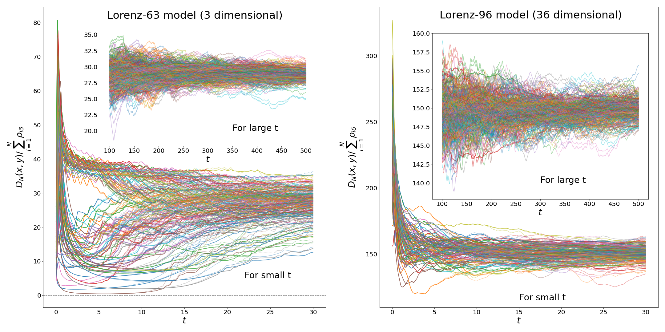
Figure 1. Dependence of $\frac{D_{N}(x,y)}{\sum_{i=0}^{N}\rho_{i\tau}}$ vs $t=N\tau$ with $\tau=0.01$ for $100$ samples. We have $t=N\tau$ with $\tau=0.01$. We chose $100$ different pairs of $(x,y)$ for five different choices of $\rho_{t}=1000,\;t+1000,\;\log(t+1000);t^{2}+1000;t^{3}+1000$. The initial conditions for the samples are randomly chosen from uniform distribution on $[-10,10]^{p}$ where the dimension $p=3$ for Lorenz 63 model (left panel) and $p=36$ for the Lorenz 96 model (right panel). The insets show the plots for large $t$. (Note that the Lyapunov time scale for both these models is $O(1)$.)

Lorenz 96 model[31]

For this model, $X=\mathbb{R}^{p}$, $\phi_{t}(u)=[x_{t}^{1}(u),x_{t}^{2}(u),...,x_{t}^{p}(u)]^{T}$ with

$$\frac{d}{dt}x_{t}^{i} =(x_{t}^{i+1}-x_{t}^{i-2})x_{t}^{i-1}-x_{t}^{i}+F$$

where, it is assumed that $x_{t}^{-1}=x_{t}^{p-1}$, $x_{t}^{0}=x_{t}^{p}$, $x_{t}^{1}=x_{t}^{p+1}$ and we again dropped the dependence of $u$. For $F=8$, this model is known to exhibit chaotic behavior.

Note that for both the models (left and right panel of Figure 1), the plots with five vary different choices of $\rho_{t}=1000,\;t+1000,\;\log(t+1000),\;t^{2}+1000,\;t^{3}+1000$ look very similar, and give a strong numerical evidence that indeed Equation (6.7) is satisfied by both Lorenz 63 and Lorenz 96 models. Providing an analytical proof of the validity of Assumption 2.4 for these models or more generally for dynamical systems of the type given in (6.4) is an interesting open question.

6.3. Qualitative understanding of Assumptions 2.4 and 4.5

In the following we will argue that a system with sensitivity to initial conditions and a positive Lyapunov exponent satisfies the Assumptions 2.4 and 4.5. We restrict ourselves to the discrete time setup and to that end, we consider a bi-Lipshitz homeomorphism, $T:X\rightarrow X$. We will see that the sensitive dependence and positiveness of Lyapunov exponent in order to argue the validity of these assumptions.

To that end, we assume that $T:X\to X$ satisfies the following properties:

1. Sensitivity to initial conditions: There exists $\delta>0$ such that for $x\in X$, $\forall\mkern 2.0mu\epsilon>0$, there exists a $\sigma$-null (zero volume) set $\mathcal{V}(x)$ such that for all $y\in B_{\epsilon}(x)\backslash\mathcal{V}$, there is $n(x,y)\in\mathbb{N}$ such that $d(T^{n(x,y)}x,T^{n(x,y)}y)>\delta$. And for $y\in\mathcal{V}(x)$, $d(T^{n}x,T^{n}y)\to 0$ as $n\to\infty$. (Note that this is a stronger notion than the one given in [21]).

2. Positive Lyapunov exponent: If $y\in B^{c}_{r}(x)\backslash\mathcal{V}$ then $d(T^{i}x,T^{i}y)>\delta$ for $i\sim\frac{1}{\lambda}\log\frac{\delta}{r}$, where $\lambda>0$ plays the role of Lyapunov exponent (Note that this property is qualitative in nature).

We give an informal argument using these properties to show that Assumption 4.5 holds. Choose $r>0$ and fix $x$ and $y$ such that $d(x,y)>r$. And also, define $a_{n}=d(T^{n}x,T^{n}y)$. We assume that $\inf_{n}(a_{n})=0$, otherwise (6.1) trivially holds for a given $x,y$ and of $T$ . And also, we assume that $\limsup_{n\to\infty}a_{n}>0$.

Let $\{n_{k}\}_{k\in\mathbb{N}}$ be a subsequence such that

$$\inf_{k}a_{n_{k}}>0\text{ and }\lim_{k\to\infty}a_{m_{k}}=0\text{ with }\{m_{k}\}_{k\in\mathbb{N}}:=\mathbb{N}\backslash\{n_{k}\}_{k\in\mathbb{N}}.$$

From the assumption that $\limsup_{n\to\infty}a_{n}>0$ and $\inf_{n}a_{n}=0$, such a $\{n_{k}\}_{k\in\mathbb{N}}$ exists. Suppose that $n_{k+1}-n_{k}\to\infty$ as $k\to\infty$, then by choosing $k$ becomes large enough, cardinality of the set $\left[n_{k},n_{k+1}\right]\cap\{m_{k}\}_{k\in\mathbb{N}}$ can be made as larger than any desired integer.

In other words, for every $\rho>0$, $1<M\in\mathbb{N}$, there exists $k_{0}$ such that for all $k\geq k_{0}$, we have

(6.9) $$n_{k+1}-n_{k}>M^{2}\text{ and }a_{m}<\rho,\;\forall\mkern 2.0mun_{k}<m<n_{k+1}.$$

Choosing $M=\frac{1}{\lambda}\log\frac{\rho}{r}$, $\bar{x}:=T^{n_{k}+1}x$ and $\bar{y}:=T^{n_{k}+1}y$, we see that this violates the assumptions on the dynamical system. To see that, we firstly note that for $i\sim\frac{1}{\lambda}\log\frac{\rho}{r}=M$, we have $d(T^{i}\bar{x},T^{i}\bar{y})>\rho$. Now for $n_{k}<m<n_{k+1}$, consider

$$a_{m}=d(T^{m-n_{k}-1}\bar{x},T^{m-n_{k}-1}\bar{y})=d(T^{m-n_{k}-1}T^{n_{k}+1}x,T^{m-n_{k}-1}T^{n_{k}+1}y)=d(T^{m}x,T^{m}y).$$

From Equation (6.9), $a_{m}<\rho$ and since $d(T^{i+n_{k}+1}{x},T^{i+n_{k}+1}{y})>\rho$ with $i\sim M$, we have a contradiction. Therefore, the supposition that $n_{k+1}-n_{k}\to\infty$ as $k\to\infty$ is false and there exist a positive constant, $J$ such that $n_{k+1}-n_{k}\leq J$ for any $k$. This implies that cardinality of the set $\{n_{k}\}_{k\in\mathbb{N}}\cap[1,2,3,...,N]$ is at least $\lfloor\frac{N}{J}\rfloor$. As a result, we have the following

$$D^{2}_{N}(x,y) \geq\delta\sum_{\begin{subarray}{c}k\in\mathbb{N},\\ n_{k}<N\end{subarray}}\rho_{n_{k}\tau}\geq\delta\sum_{i=0}^{\lfloor\frac{N}{J}\rfloor}\rho_{i\tau}\geq\delta G\left(\alpha,J\right)\sum_{i=0}^{N}\rho_{i\tau},$$

where $G\left(\alpha,J\right)>0$ depends only on $\alpha$ and $J$. The above inequalities follow from non-decreasing property of $\rho_{t}$, applying the lowest bound to any sum up to first $\lfloor\frac{N}{J}\rfloor$ terms of an subsequence of a non-decreasing sequence and the form of $\rho_{t}$.

To summarize, in the current section, we studied various filtering models that satisfy the assumptions of Sections 2 and  4.

7. Conclusions

The problem that we studied in this paper is the asymptotic stability of the nonlinear filter with deterministic dynamics. In order to establish stability, we first proved, in Theorem 3.1, an accuracy or consistency result for the smoother, i.e., the convergence of the conditional distribution of the initial condition given observations. We used this result to prove the stability of the filter in Theorem 3.8. Using essentially identical methods, we also established the accuracy of the smoother (Theorem 4.8) and the stability of the filter (Theorem 4.10) in the case of discrete time.

The main assumptions used in proving these results are quite natural as discussed in Section 2.4, and are indeed satisfied by two large classes of dynamical systems, as discussed in Section 6. In particular, these assumptions are valid for a class of diffeomorphisms of compact manifolds with appropriate enough observation function, as well as a class of nonlinear differential equations that includes models such as the Lorenz models (using numerical evidence for Assumption 2.4).

There are various possible directions for further studies. Theorems 3.8 and 4.10 do not give any rate of convergence, because of the use of Martingale convergence theorem, and it would be interesting to find finer methods that may give the rate of convergence, such as those [10, Section 4.3] available for the convergence of covariance of the filter for linear models. Further, partly because of the use of convergence of the smoother to prove filter stability, our results do not give much information about the structure of the asymptotic filtering distribution, such as that which is available [10, Sections 4.3, 5], [37, Remark 3.2] for the linear filter. We hope that further investigations in this direction will lead to efficient numerical implementations of the filter for deterministic dynamics, especially for high dimensional systems.

References

• Anderson and Moore [1969] Brian Anderson and JB Moore. New results in linear system stability. SIAM Journal on Control, 7(3):398–414, 1969.
• Apte et al. [2007] A. Apte, M. Hairer, A.M. Stuart, and J. Voss. Sampling the posterior: an approach to non-Gaussian data assimilation. Physica D, 230:50–64, 2007.
• Asch et al. [2016] Mark Asch, Marc Bocquet, and Maëlle Nodet. Data Assimilation: Methods, Algorithms, and Applications. SIAM, 2016.
• Atar [1998] Rami Atar. Exponential stability for nonlinear filtering of diffusion processes in a noncompact domain. The Annals of Probability, 26(4):1552–1574, 1998.
• Atar and Zeitouni [1997] Rami Atar and Ofer Zeitouni. Exponential stability for nonlinear filtering. Annales de l’Institut Henri Poincare (B) Probability and Statistics, 33(6):697–725, 1997.
• Bain and Crisan [2008] Alan Bain and Dan Crisan. Fundamentals of stochastic filtering, volume 60. Springer Science & Business Media, 2008.
• Barreira and Pesin [2013] Luis Barreira and Ya B Pesin. Introduction to smooth ergodic theory, volume 148. American Mathematical Soc., 2013.
• Billingsley [1999] Patrick Billingsley. Convergence of probability measures. Wiley Series in Probability and Statistics: Probability and Statistics. John Wiley & Sons Inc., second edition, 1999.
• Bishop and Del Moral [2017] Adrian N Bishop and Pierre Del Moral. On the stability of Kalman–Bucy diffusion processes. SIAM Journal on Control and Optimization, 55(6):4015–4047, 2017.
• Bocquet et al. [2017] Marc Bocquet, Karthik S Gurumoorthy, Amit Apte, Alberto Carrassi, Colin Grudzien, and Christopher KRT Jones. Degenerate Kalman filter error covariances and their convergence onto the unstable subspace. SIAM/ASA Journal on Uncertainty Quantification, 5(1):304–333, 2017.
• Budhiraja [2003] Amarjit Budhiraja. Asymptotic stability, ergodicity and other asymptotic properties of the nonlinear filter. Annales de l’IHP Probabilités et statistiques, 39(6):919–941, 2003.
• Budhiraja and Ocone [1997] Amarjit Budhiraja and Daniel Ocone. Exponential stability of discrete-time filters for bounded observation noise. Systems & Control Letters, 30(4):185–193, 1997.
• Budhiraja and Ocone [1999] Amarjit Budhiraja and Daniel Ocone. Exponential stability in discrete-time filtering for non-ergodic signals. Stochastic processes and their applications, 82(2):245–257, 1999.
• Carrassi et al. [2018] Alberto Carrassi, Marc Bocquet, Laurent Bertino, and Geir Evensen. Data assimilation in the geosciences: An overview of methods, issues, and perspectives. WIREs Clim Change, 9(5):e535, 2018.
• [15] Frédéric Cérou. Long time asymptotics for some dynamical noise free non-linear filtering problems , new cases. [Research Report] RR-2541, INRIA. 1995. inria-00074137.
• Cérou [2000] Frédéric Cérou. Long time behavior for some dynamical noise free nonlinear filtering problems. SIAM Journal on Control and Optimization, 38(4):1086–1101, 2000.
• Chigansky et al. [2009] P Chigansky, R Liptser, and R Van Handel. Intrinsic methods in filter stability. Handbook of Nonlinear Filtering, 2009.
• [18] Pavel Chigansky. Stability of nonlinear filters: A survey, 2006. Mini-course lecture notes, Petropolis, Brazil.
• Clark et al. [1999] JMC Clark, Daniel Ocone, and C Coumarbatch. Relative entropy and error bounds for filtering of Markov processes. Mathematics of Control, Signals and Systems, 12(4):346–360, 1999.
• D’Aristotile et al. [1988] Anthony D’Aristotile, Persi Diaconis, and David Freedman. On merging of probabilities. Sankhyā Ser. A, 50(3):363–380, 1988.
• Glasner and Weiss [1993] Eli Glasner and Benjamin Weiss. Sensitive dependence on initial conditions. Nonlinearity, 6(6):1067–1075, 1993.
• Gollwitzer [1969] H. E. Gollwitzer. A note on a functional inequality. Proceedings of the American Mathematical Society, 23(3):642–647, 1969.
• Gurumoorthy et al. [2017] Karthik S Gurumoorthy, Colin Grudzien, Amit Apte, Alberto Carrassi, and Christopher KRT Jones. Rank deficiency of Kalman error covariance matrices in linear time-varying system with deterministic evolution. SIAM Journal on Control and Optimization, 55(2):741–759, 2017.
• Kallianpur [1980] Gopinath Kallianpur. Stochastic filtering theory, volume 13. Springer Science & Business Media, 1980.
• Katok and Hasselblatt [1996] Anatole Katok and Boris Hasselblatt. Introduction to the modern theory of dynamical systems, volume 54. Cambridge university press, 1996.
• Kelly et al. [2014] David TB Kelly, KJH Law, and Andrew M Stuart. Well-posedness and accuracy of the ensemble Kalman filter in discrete and continuous time. Nonlinearity, 27(10):2579, 2014.
• Koro [accessed November 6, 2020] Koro. Uniform expansivity (https://planetmath.org/uniformexpansivity), accessed November 6, 2020. URL https://planetmath.org/UniformExpansivity.
• Law et al. [2015] Kody Law, Andrew Stuart, and Kostas Zygalakis. Data Assimilation. Springer, 2015.
• Ledoux [1996] Michel Ledoux. Isoperimetry and Gaussian analysis. In Lectures on probability theory and statistics, pages 165–294. Springer, 1996.
• Lorenz [1963] Edward N Lorenz. Deterministic nonperiodic flow. Journal of the atmospheric sciences, 20(2):130–141, 1963.
• Lorenz [1996] Edward N Lorenz. Predictability: A problem partly solved. In Proc. Seminar on predictability, volume 1, 1996.
• McDonald and Yuksel [2018] Curtis McDonald and Serdar Yuksel. Stability of non-linear filters and observability of stochastic dynamical systems. arXiv preprint arXiv:1812.01772, 2018.
• Ni and Zhang [2016] Boyi Ni and Qinghua Zhang. Stability of the Kalman filter for continuous time output error systems. Systems & Control Letters, 94:172–180, 2016.
• Ocone [1999] Daniel Ocone. Asymptotic stability of Beneš filters. Stochastic analysis and applications, 17(6):1053–1074, 1999.
• Ocone and Pardoux [1996] Daniel Ocone and Etienne Pardoux. Asymptotic stability of the optimal filter with respect to its initial condition. SIAM Journal on Control and Optimization, 34(1):226–243, 1996.
• Palmer [2019] TN Palmer. Stochastic weather and climate models. Nature Reviews Physics, 1(7):463–471, 2019.
• Reddy et al. [2019] Anugu Sumith Reddy, Amit Apte, and Sreekar Vadlamani. Asymptotic properties of linear filter for noise free dynamical system. arXiv preprint arXiv:1901.00307, 2019.
• Reich and Cotter [2015] Sebastian Reich and Colin Cotter. Probabilistic forecasting and Bayesian data assimilation. Cambridge University Press, 2015.
• Shub [1986] Michael Shub. Global stability of dynamical systems. Springer Science & Business Media, 1986.
• Van Handel [2007] Ramon Van Handel. Filtering, Stability, and Robustness. PhD thesis, California Institute of Technology, 2007.
• Van Handel [2009] Ramon Van Handel. Observability and nonlinear filtering. Probability theory and related fields, 145(1-2):35–74, 2009.
• Van Handel [2010] Ramon Van Handel. Nonlinear filtering and systems theory. In Proceedings of the 19th International Symposium on Mathematical Theory of Networks and Systems (MTNS semi-plenary paper), 2010.
• Walters [1982] Peter Walters. An introduction to ergodic theory, volume 79. Springer Science & Business Media, 1982.
• Williams [1991] David Williams. Probability with Martingales. Cambridge mathematical textbooks. Cambridge University Press, 1991.
• Xiong [2008] Jie Xiong. An introduction to stochastic filtering theory, volume 18. Oxford University Press on Demand, 2008.