Robust boundary flow in chiral active fluid

Abstract

We perform experiments on an active chiral fluid system of self-spinning rotors in confining boundary. Along the boundary, actively rotating rotors collectively drives a unidirectional material flow. We systematically vary rotor density and boundary shape; boundary flow robustly emerges under all conditions. Flow strength initially increases then decreases with rotor density (quantified by area fraction $\phi$); peak strength appears around a density $\phi=0.65$. Boundary curvature plays an important role: flow near a concave boundary is stronger than that near a flat or convex boundary in the same confinements. Our experimental results in all cases can be reproduced by a continuum theory with single free fitting parameter, which describes the frictional property of the boundary. Our results support the idea that boundary flow in active chiral fluid is topologically protected; such robust flow can be used to develop materials with novel functions.

I Introduction

Active matter is composed of constituent units individually powered by internal or external energy sources. In majority of current studies, local energy injection drives constituent unit’s linear motion (Marchetti et al., 2013). In these systems, a wide range of phenomena has been reported, including emergent collective motion (Bricard et al., 2013; Kumar et al., 2014), pattern formation (Riedel et al., 2005; Cates et al., 2010; Farrell et al., 2012; Bricard et al., 2015) and phase segregation without attraction (Fily and Marchetti, 2012; Redner et al., 2013; Stenhammar et al., 2013). Besides linear motion, local energy injection can also cause constituent unit to actively rotate. Biological examples of such chiral active matter include rotating bacteria (Petroff et al., 2015; Chen et al., 2015), circling bacteria (Diluzio et al., 2005; Lauga et al., 2006; Leonardo2011) and sperm cells (Friedrich and Ju, 2007; Riedel et al., 2005) near surfaces, and magnetotactic bacteria in rotating fields (Erglis, 2007; Cebers, 2011). Artificial chiral active systems have also been developed, such as colloids (Yan et al., 2015a, b; Maggi et al., 2015; Kokot et al., 2017; Xie et al., 2019; Aubret et al., 2018; Soni et al., 2019), millimeter-scale magnets(Grzybowski et al., 2000; Grzybowski and Whitesides, 2002) and rotating granular particles (Tsai et al., 2005; Scholz et al., 2018; Farhadi et al., 2018; Workamp et al., 2018). Multiple numerical and theoretical studies on chiral active fluid have been carried out (Lenz et al., 2003; Tsai et al., 2005; Furthauer et al., 2013; Nguyen et al., 2014; Spellings et al., 2015; Goto and Tanaka, 2015; Aragones and Steimel, 2016; Yeo et al., 2015; Reichhardt and Reichhardt, 2019).

Interacting active rotors can form a range of collective phenomena. One of such phenomena is unidirectional material flow localized at rotor/solid (Tsai et al., 2005; van Zuiden et al., 2016), rotor/liquid (Soni et al., 2019) and rotor phase boundaries (Nguyen et al., 2014; Scholz et al., 2018). A continuum theory was developed to reproduce boundary flow in a driven granular system in a circular confinement (Tsai et al., 2005). Later, the same theory was compared with numerical data of confined rotors (van Zuiden et al., 2016). Recently, Dasbiswas, Mandadapu, and Vaikuntanathan (Dasbiswas et al., 2018) studied topological properties of the continuum theory; they showed that the emergence of the boundary flow in active chiral fluid can be understood as an example of topological protection at boundary (Dasbiswas et al., 2018) and that the boundary flow is insensitive to boundary interactions and highly resistant to perturbations. Similar robustness has been extensively studied in many topologically nontrivial systems, such as mechanical lattice (Kane and Lubensky, 2013; Paulose et al., 2015; Lubensky et al., 2015), electronic (Hasan and Kane, 2010) and photonic (Haldane and Raghu, 2008) systems.

Here, we investigate boundary flow of individually-driven, rotating particles in confining boundaries by experiment and theory. Our experiments show that boundary flow robustly emerges in all cases of various rotor densities and boundary shapes. To facilitate the comparison between experiments and theory, we use experimental observations to simplify the continuum theory (Tsai et al., 2005) and carry out independent experiments to identify model parameters. Eventually, our experimental results in all cases can be reproduced by the continuum theory with single free fitting parameter, which describes the frictional property of the boundary.

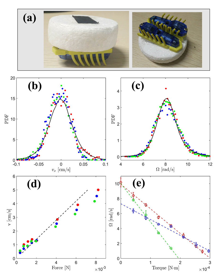
Figure 1: Construction and properties of single rotor. (a) two images showing a rotor made of two Hexbug robots and a foam disk. (b-c) Probability distribution functions of linear velocity and spin rate. Lines and symbols represent average results over 40 rotors and data from individual rotors, respectively. (d-e) Rotor responses to external force and torque. Lines are linear fits to experimental data (symbols).

II Experimental methods and results

Our rotor ($m=15.3\pm 0.2$g in mass) is driven by two Hexbug robots. Each Hexbug, 4.3 cm long and 1.2 cm wide, houses a 1.5V button cell battery that drives a vibration motor; we use fresh batteries in each new experiment and run experiments for less than 20 minutes to prevent battery power degrading. Hexbug body is supported by twelve flexible legs that all bends slightly backwards. When turned on, the vibration motor sets Hexbug into forward hopping motion on a solid (PMMA) substrate (Dauchot and Demery, 2019; Li and Zhang, 2013). As shown in Fig. 1(a), two Hexbug robots in a rotor are glued to a foam disk ( radius $a=2.5$cm ) in opposite directions; they can generate a torque that spins the rotor with a spin rate about $\varOmega_{0}\approx 8.4$ rad/s, cf. Fig. 1(c). Rotors and the substrate are carefully balanced so that translational motion of an isolated rotor is suppressed, cf. Fig. 1(b). Our rotors respond linearly to external force and torque, as shown in Fig. 1(d-e); detailed description of these experiments can be found in supplementary information.

To observe localized boundary flow, we confine rotors with solid boundaries which are precisely machined by a laser-cutter and covered with smooth tapes to reduce friction, cf. Fig. 2(a). Different numbers of rotors are used to vary density. Rotor motion is recorded by a digital camera at 30 frames per second; we use standard particle tracking method to measure rotor translation and rotation from recorded videos. Experimental results obtained in both axisymmetric and non-axisymmetric confinements are discussed in detail below.

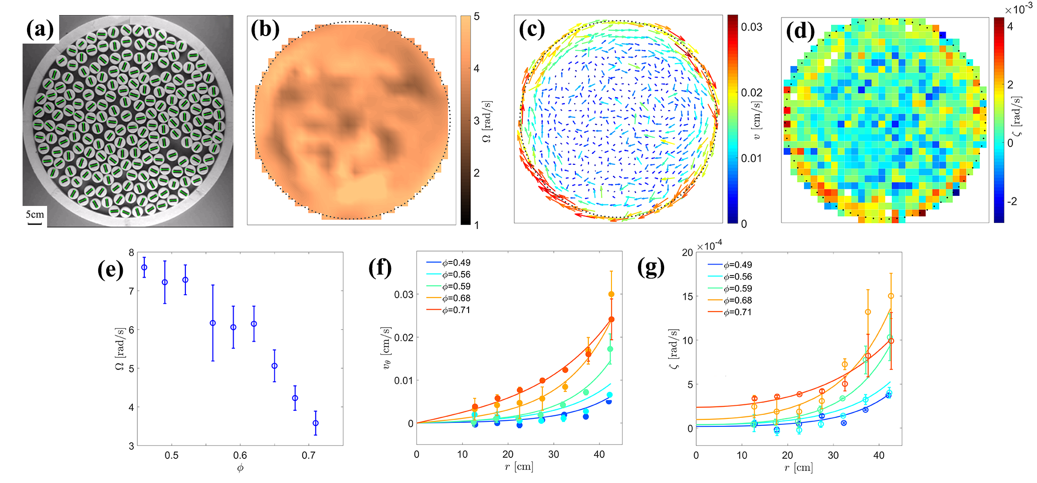
Figure 2: Results in a circular confinement. (a) Snapshot from an experiment with $\phi=$0.68. Black markers on rotors are used to facilitate particle tracking. Coarsen-grained fields ($\varOmega(\vec{r})$, $\vec{v}(\vec{r})$ and $\zeta(\vec{r})$) from the same experiment are shown in (b-d); Dotted line marks the effective boundary of the space accessible to the rotor center. (e) Density dependence of averaged spin rate $\Omega$. (f-g) Radial profiles of $v_{\theta}(r)$ and $\zeta(\vec{r})$. symbols and lines represent experimental and numerical results, respectively.

II.1 Axisymmetric boundary

We start from a circular boundary with a radius $R_{c}=45$ cm, cf. Fig. 2(a). Five different numbers of rotors are used: $N=$ 160,180,190,220 and 230; the corresponding area fraction $\phi\equiv\frac{N\pi a^{2}}{\pi R_{c}^{2}}$ are 0.49, 0.56, 0.59, 0.68 and 0.71, respectively. Typical system dynamics can be seen in supplementary movie S1: while spinning rotors interact with neighbors and boundary, part of their angular momentum is converted to linear momentum, which is reflected by rotors’ translational motion; rotor translation is most pronounced near the boundary and is in the clockwise direction.

We measure spin rate $\varOmega$ and velocity $\vec{v}$ of each rotor and average measured results in 1.5$\times$1.5 c${\textstyle\textrm{m}}^{2}$ bins. As shown in Fig. 2(b) and (e), coarse-grained spin rate $\varOmega(\vec{r})$ has an approximately uniform spatial distribution and its mean value decreases as the rotor density increases, cf. Fig. 2(e); this is mainly caused by the frictional slides of neighbors. Coarsen-grained linear velocity field $\vec{v}(\vec{r})$ is shown in Fig. 2(c); local angular velocity $\zeta(\vec{r})\equiv\frac{1}{2}\left(\nabla\times\vec{v}(\vec{r})\right)_{z}$ computed and plotted in Fig. 2(d). By averaging data in concentric annuli between $r-a$ and $r+a$, we can get radial profiles of $v_{\theta}(r)$ and $\zeta(r)$. Data in Fig. 2(f-g) show that localized boundary flow emerges under all density conditions with different strength.

We add an inner boundary ($15$ cm in radius) to the system; this makes a ring-shaped confinement, as shown in Fig. 3(a). As in the case of circular boundary, coarsen-grained fields, $\vec{v}(\vec{r})$ and $\zeta(\vec{r})$, and their radial profiles are measured and plotted in Fig. 3. From these data, we see that, in addition to the clockwise flow along the outer boundary, a counter-clockwise flow emerges near the inner boundary, which is weaker and can most clearly seen from $v_{\theta}(r)$ profiles in Fig. 3(c).

II.2 Non-axisymmetric boundary

We further investigate two cases of non-axisymmetric boundary: capsule-shaped and U-shaped confinements as shown in Fig. 4(a) and (d). In both cases, curvature changes along the boundary and affects the strength of boundary flow. To quantify this point, linear velocity and local angular velocity at representative points, square and circular symbols in (a) and (d), are computed at six rotor densities. Data in Fig. 4(b-c) show boundary flow near concave boundary (red symbols) is stronger than that (blue symbols) near a flat region. In the case of U-shaped confinement, cf. Fig. 4 (d-f) and supplementary movie S2, concave boundary(red symbols) generates stronger flow than convex boundary (blue symbols). We also discover that the flow velocity peaks near the density $\phi=0.65$ in both cases, as shown in Fig. 4(b) and (e).

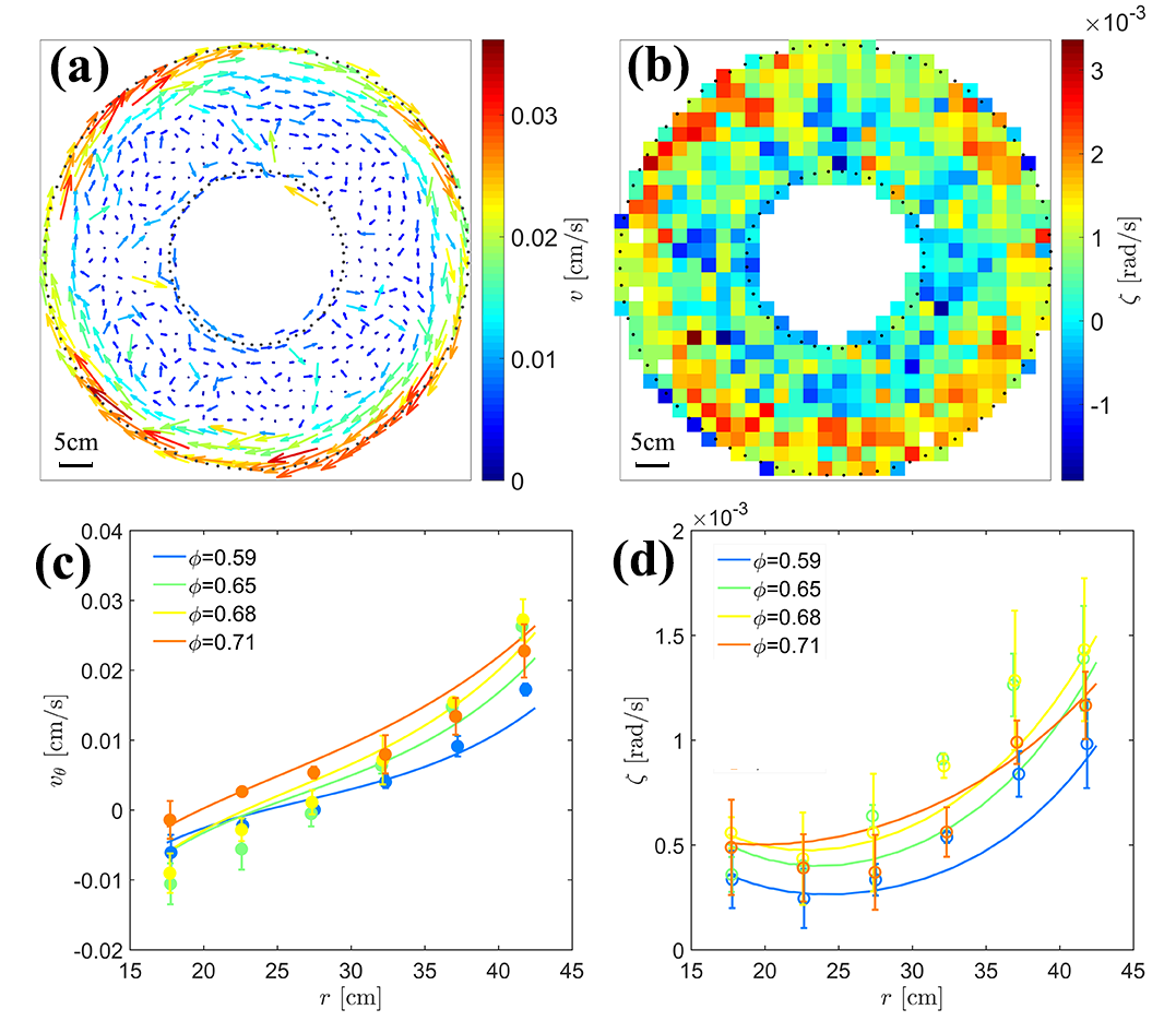
Figure 3: Results in a ring-shaped confinement. (a) velocity field and (b) local collective angular velocity field measured in experiments with $\phi=$0.68. Radial profiles of $v_{\theta}(r)$ and $\zeta(\vec{r})$ are shown in (c-d); symbols and lines represent experimental and numerical results, respectively.

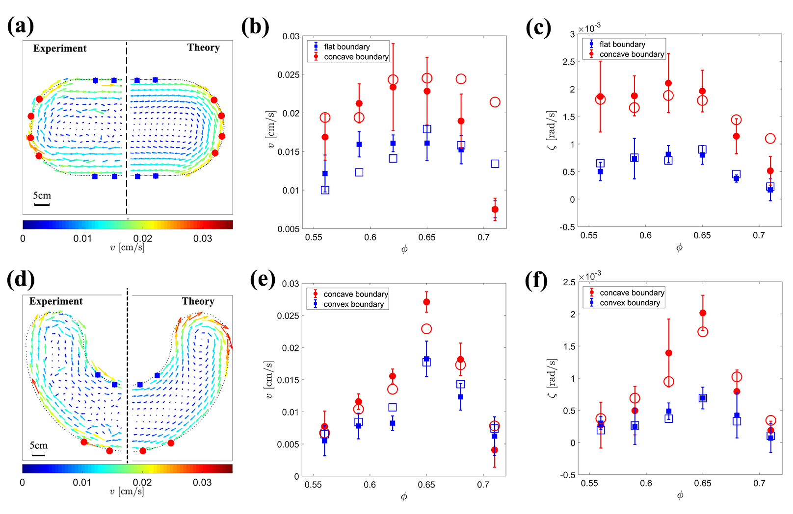
Figure 4: Results in two non-axisymmetric cases: (a-c) capsule-shaped and (d-f) U-shaped confinements. Effective boundary of rotor centers in two cases is represented by dotted line in (a) and (d). Experimentally measured velocity fields with $\phi=$0.68 are shown in the left half of (a) and (d) with corresponding theoretical prediction on the right. Averaged velocity and local angular velocity at representative points, marked by symbols in (a) and (d), are computed at different densities and plotted in (b-c) and (e-f); experimental and theoretical results are represented by filled and empty symbols, respectively.

III Theoretical analysis of experimental results

III.1 Continuum theory

To understand experimental results in Figs. 1-4, we use a continuum theory developed by Tsai and coauthors (Tsai et al., 2005). The theory describes the conservation laws of the following hydrodynamic variables: the mass density $\rho(\vec{r},t)$, the momentum density $\rho\vec{v}(\vec{r},t)$ and the angular momentum density $I\varOmega(\vec{r},t)$, where $I$ is the moment of inertial density. The first continuum equation describes mass conservation:

$$\frac{\partial\rho}{\partial t}+\nabla\cdot(\rho\vec{v})=0,$$ (1)

where the mass density $\rho$ is proportional to the area fraction of rotors $\phi$: $\rho=\frac{m}{\pi a^{2}}\phi$. Rotor density in our experiments is spatially homogeneous, cf. Fig. 2(a) and Fig. S2, which allows us simplify Eq. (1) as :

$$\nabla\cdot\vec{v}=0.$$ (2)

The angular momentum of rotors is conserved:

$$ID_{t}\varOmega=D_{\varOmega}\nabla^{2}\varOmega-\Gamma^{\varOmega}\varOmega-\Gamma(\varOmega-\zeta)+\tau,$$ (3)

where $D_{t}\equiv\partial_{t}+\vec{v}\cdot\nabla$ is convective derivative, $D_{\varOmega}$ is the angular momentum diffusion constant, $\Gamma^{\varOmega}$ is the angular friction coefficient due to rotor-substrate interaction, $\Gamma$ is spin-velocity coupling constant, and $\tau$ stands for driving torque density field experienced by the rotors. We can simplify Eq. (3) as

$$\tau=\Gamma^{\varOmega}\varOmega+\Gamma\varOmega$$

by the following experimental observations: 1) our system in steady state; 2) homogeneous angular momentum field $\varOmega$ (Fig. 2b); 3) local angular velocity $\zeta$ is much less than spin rate $\varOmega$ (Fig. 2g and 3d). Under low density condition, isolated rotors experiences little coupling to others, i.e. $\Gamma=0$, we have spin rate for isolated rotors:

$$\varOmega_{0}=\frac{\tau}{\Gamma^{\varOmega}}.$$

Combining two equations above, we have the following relation:

$$\frac{\varOmega}{\varOmega_{0}}=\frac{\Gamma^{\varOmega}/\varGamma}{\Gamma^{\varOmega}/\varGamma+1}.$$ (4)

Momentum conservation requires:

$$\rho D_{t}\vec{v}=-\nabla p+\eta\nabla^{2}\vec{v}-\Gamma^{v}\vec{v}+\frac{\Gamma}{2}\epsilon\nabla(\varOmega-\zeta),$$ (5)

where $\eta$ is the shear viscosity, $\Gamma^{v}$ is the linear friction coefficient, and $\epsilon$ is 2D antisymmetric symbol. The odd viscosity has been ignored in our system for quite large damping coefficient $\Gamma^{v}$ (Banerjee et al., 2017). With a steady-state assumption, we take the curl of Eq. (5):

$$\left((4\eta+\Gamma)\nabla^{2}-4\Gamma^{v}\right)\zeta-\Gamma\nabla^{2}\varOmega=0.$$ (6)

The above equation can be further simplified by assuming a homogeneous angular momentum field $\varOmega$ and weak coupling $\Gamma\ll\eta$ (see Fig. 5b); we end up with the following equation:

$$\left(\nabla^{2}-\frac{\Gamma^{v}}{\eta}\right)(\nabla\times\vec{v})_{z}=0.$$ (7)

III.2 Boundary conditions

Eq. (2) and Eq. (7) can be solved with proper boundary conditions. The boundary is characterized by a local outward normal vector, $\hat{r}$, and a tangential direction, $\hat{\theta}$; the local radius curvature is denoted as $R$ with the convention that a concave boundary has a positive radius of curvature. A rigid wall requires the radial velocity component to be zero:

$$v_{r,B}=0,$$ (8)

where the subscript “$B$” stands for the boundary of the occupied region for rotor centers, as shown by the dotted line in Fig. 2(b-d) for circular boundary. The second boundary condition arises from the fact that rotors also experience a frictional force from the boundary; this leads to a tangential-radial component of the stress tensor:

$$\sigma_{\theta r,B}=f_{B},$$ (9)

where $f_{B}$ is an effective boundary friction on unit length. We assume that $f_{B}$ is proportional to the shear stress from the spin-velocity coupling:

$$f_{B}=-k\Gamma\varOmega,$$ (10)

As the friction of rotor-rotor and rotor-boundary have similar dependence on $\phi$, the proportion factor $k$ in Eq. 10 is treated as a constant in a given experiment. We express $\sigma_{\theta r}$ in velocity components, combine Eqs. (8-10) and obtain the following boundary condition (See supplementary information for detailed discussions):

$$\left(\zeta-\frac{v_{\theta}}{R}\right)_{B}=\frac{\varGamma}{4\eta}(1-2k)\varOmega_{B}.$$ (11)

III.3 Determination of model parameters

Fig. 1(d) and (e) shows linear responses of isolated rotors to external force and torque. By measuring slopes of data in these plots, we extracted linear and angular frictional coefficient for isolated rotors: $\gamma^{v}=0.14$ kg/s and $\gamma^{\varOmega}=0.32$ kg $\textrm{cm}{}^{2}$/s. These two quantifies are related to $\Gamma^{v}$ and $\Gamma^{\varOmega}$ as : $\Gamma^{v}=\rho\gamma^{v}=\frac{m}{\pi a^{2}}\phi\gamma^{v}$ and $\Gamma^{\varOmega}=\rho\gamma^{\varOmega}=\frac{m}{\pi a^{2}}\phi\gamma^{\varOmega}$; this leads to $\Gamma^{\varOmega}/\Gamma^{v}=0.44$ cm^-2 for all densities.

Eq. (4) relates spin rate $\Omega$ to the ratio of angular frictional coefficient $\Gamma^{\varOmega}$ to coupling constant $\Gamma$. Our experiments show that spin rate $\Omega$ decreases with increasing rotor density, cf. Fig. 2(e). From such data, we can use Eq. (4) to measure the ratio $\Gamma^{\varOmega}/\Gamma$ in different confinements and different densities. Results are plotted in Fig. 5(a), showing a monotonic decrease with area fraction $\phi$; collapse of all data on a single curve demonstrates that this ratio depends weakly on boundary shape and is a bulk property of the system.

We can estimate the ratio $\varGamma/\eta$ from stress boundary condition, Eq. 11, by rewriting the equation as

$$\frac{\varGamma}{\eta}=\frac{4\left(\zeta-v_{\theta}/R\right)_{B}}{(1-2k)\varOmega_{B}}.$$

Quantities in the above equation, $\zeta,v_{\theta},\text{and }\Omega$ at boundary, can be measured directly from experiments. Therefore, for any given proportion constant $k$, we can compute $\frac{\varGamma}{\eta}$ along the boundary then average computed values, which depends weakly on local curvature. Averaged results for $\frac{\varGamma}{\eta}$ obtained with $k=0.4$ are plotted in Fig. 5(b). $\frac{\varGamma}{\eta}$ results from different confinements approximately collapse onto a single curve and show a peak around density $\phi=0.65$, where peak boundary flow in Fig. 4(b) and (e) appears. Fig. 5(b) shows that spin-velocity coupling is weak in our system, with a coupling constant $\Gamma$ two-order magnitude smaller than the shear viscosity $\eta$.

III.4 Comparison between theoretical and experimental results

With the process in the above section, we can estimate three parameter ratios in every experiment. From these ratios, the only parameter in Eq. (7) can be determined:

$$\frac{\Gamma^{v}}{\eta}=\left(\frac{\Gamma^{v}}{\Gamma^{\varOmega}}\right)\left(\frac{\Gamma^{\varOmega}}{\varGamma}\right)\left(\frac{\varGamma}{\eta}\right).$$ (12)

Because spin rate $\Omega$ is spatially homogeneous, we set its boundary value in Eq. (11) $\Omega_{B}$ as the measured spin rate in bulk. The proportion constant $k$ is treated as an adjusting parameter. For a given $k$ value, we use a finite-element package (COMSOL) to solve Eq. (2) and Eq. (7) with boundary conditions Eq. (8) and Eq. (11) for steady flow $\vec{v}(\vec{r},t)$ in all experiments. In a typical calculation, more than 10,000 finite elements are used to ensure convergence. Detailed numerical results for a capsule-shaped confinement can be found in Fig. S4.

We compare theoretical results to experiments and find that $k=0.4$ yields the best overall agreement. All theoretical results in Figs. 2-4 are computed with $k=0.4$. In the case of circular boundary, theoretical solutions correctly capture the spatial lengthscale and density dependence of the boundary flow, as shown in Fig. 2. In ring geometry, Fig. 3, continuum theory predicts the reversal of flow direction as one moves from the inner to outer boundary and non-monotonic behavior in local angular velocity, $\zeta$. In non-axisymmetric cases, main features of steady flow are well captured in theoretical solutions, especially how flow depends on local curvature and rotor density. Effect of local curvature is manifested through the stress boundary condition, Eq. (11), see detailed discussion in supplementary information. Rotor density enters the theory through model parameters shown in Fig. 5.

We note that Fig. 4 (b) and (e) show some deviation of theoretical results from experiments at high densities. This is likely caused by transient jamming of densely packed rotors in experiments, which are not captured in the current fluid-based continuum theory. Transient jamming and associated elastic stress can also explain the sharp drop of boundary flow beyond density $\phi=0.65$, cf. Fig. 4 (b) and (e).

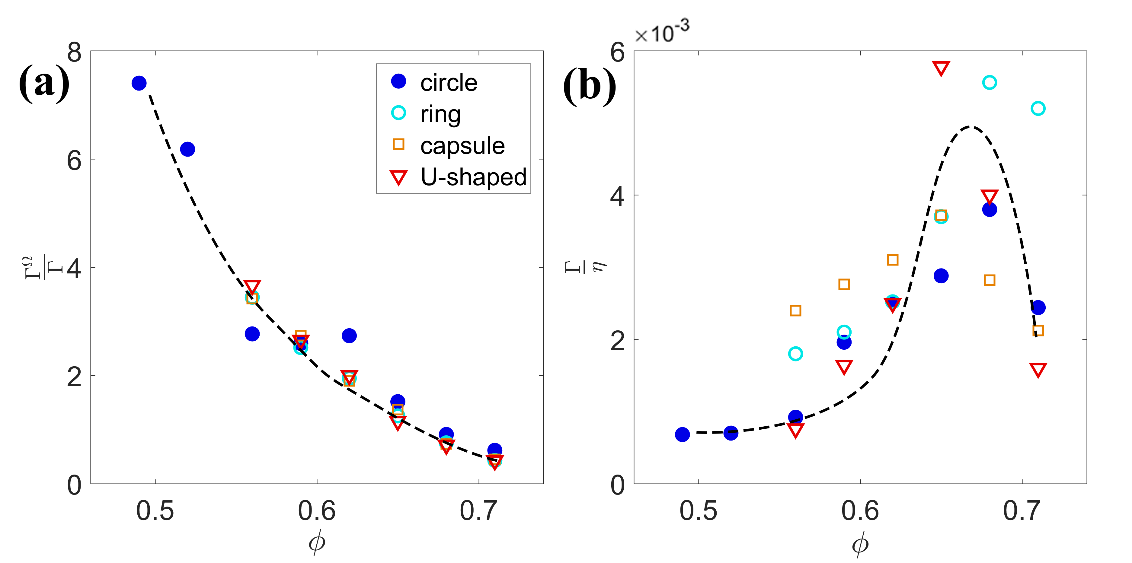
Figure 5: Density dependence of two parameter ratios extracted from experiments: (a) $\frac{\Gamma^{\varOmega}}{\varGamma}$ and (b) $\frac{\varGamma}{\eta}$. Data from different confinements are shown by symbols. Dashed lines are a guide to the eye.

IV Conclusion and discussion

We have studied collective dynamics of rotors in various confining boundaries and density conditions. Actively rotating rotors collectively drives a unidirectional material flow along boundary. Boundary flow robustly emerges in all experiments with different rotor densities and boundary shapes. We showed that flow strength initially increases then decreases with rotor density and peak strength appears around a density $\phi=0.65$. Boundary curvature plays an important role: flow near a concave boundary (with a positive radius of curvature) is stronger than that near a flat or convex boundary in the same confinements. We corroborate experimental measurements with a theoretical analysis based on a continuum theory, which is simplified under our experimental conditions; independent experimental measurements were used to determine transport coefficients in the theory. We demonstrated that our experimental results in all cases were quantitatively reproduced by the theory with single free fitting parameter, which describes the frictional property of the boundary. Our experimental and theoretical results support the idea that emergence of robust boundary flow in chiral active matter is an example of topological protection phenomena in dissipative system (Dasbiswas et al., 2018). Topological nature of the boundary flow may allow us to develop new materials with novel and robust functions.

References

- Marchetti et al. (2013) M. C. Marchetti, J. F. Joanny, S. Ramaswamy, T. B. Liverpool, J. Prost, M. Rao, and R. A. Simha, Rev. Mod. Phys. 85, 1143 (2013).
- Bricard et al. (2013) A. Bricard, J.-b. Caussin, N. Desreumaux, O. Dauchot, and D. Bartolo, Nature 503, 95 (2013).
- Kumar et al. (2014) N. Kumar, H. Soni, S. Ramaswamy, and A. K. Sood, Nat. Commun. 5, 1 (2014).
- Riedel et al. (2005) I. H. Riedel, K. Kruse, and J. Howard, Science 309, 300 (2005).
- Cates et al. (2010) M. E. Cates, D. Marenduzzo, I. Pagonabarraga, and J. Tailleur, Proc. Natl. Acad. Sci. 107, 11715 (2010).
- Farrell et al. (2012) F. Farrell, M. C. Marchetti, D. Marenduzzo, and J. Tailleur, Phys. Rev. Lett. 108, 248101 (2012).
- Bricard et al. (2015) A. Bricard, J.-B. Caussin, D. Das, C. Savoie, V. Chikkadi, K. Shitara, O. Chepizhko, F. Peruani, D. Saintillan, and D. Bartolo, Nat. Commun. 6, 7470 (2015).
- Fily and Marchetti (2012) Y. Fily and M. C. Marchetti, Phys. Rev. Lett. 108, 235702 (2012).
- Redner et al. (2013) G. S. Redner, M. F. Hagan, and A. Baskaran, Phys. Rev. Lett. 110, 055701(5) (2013).
- Stenhammar et al. (2013) J. Stenhammar, A. Tiribocchi, R. J. Allen, D. Marenduzzo, and M. E. Cates, Phys. Rev. Lett. 111, 145702(5) (2013).
- Petroff et al. (2015) A. P. Petroff, X.-L. Wu, and A. Libchaber, Phys. Rev. Lett. 114, 158102 (2015).
- Chen et al. (2015) X. Chen, X. Yang, M. Yang, and H. P. Zhang, Europhys. Lett. 111, 54002 (6 pp.) (2015).
- Diluzio et al. (2005) W. R. Diluzio, L. Turner, M. Mayer, P. Garstecki, D. B. Weibel, H. C. Berg, and G. M. Whitesides, Nature 435, 1271 (2005).
- Lauga et al. (2006) E. Lauga, W. R. Diluzio, G. M. Whitesides, and H. A. Stone, Biophys. J. 90, 400 (2006).
- Friedrich and Ju (2007) B. M. Friedrich and F. Ju, Proc. Natl. Acad. Sci. 104, 13256 (2007).
- Erglis (2007) K. Erglis, Biophys. J. 93, 1402 (2007).
- Cebers (2011) A. Cebers, J. Magn. Magn. Mater. 323, 279 (2011).
- Yan et al. (2015a) J. Yan, S. C. Bae, and S. Granick, Soft Matter 11, 147 (2015a).
- Yan et al. (2015b) J. Yan, S. C. Bae, and S. Granick, Adv. Mater. 27, 874 (2015b).
- Maggi et al. (2015) C. Maggi, F. Saglimbeni, M. Dipalo, F. D. Angelis, and R. D. Leonardo, Nat. Commun. 6, 1 (2015).
- Kokot et al. (2017) G. Kokot, S. Das, R. G. Winkler, G. Gompper, I. S. Aranson, and A. Snezhko, Proc. Natl. Acad. Sci. 114, 12870 (2017).
- Xie et al. (2019) H. Xie, M. M. Sun, X. J. Fan, Z. H. Lin, W. N. Chen, L. Wang, L. X. Dong, and Q. He, Sci. Rob. 4, eaav8006 (2019).
- Aubret et al. (2018) A. Aubret, M. Youssef, S. Sacanna, and J. Palacci, Nat. Phys. (2018).
- Soni et al. (2019) V. Soni, E. S. Bililign, S. Magkiriadou, S. Sacanna, D. Bartolo, M. J. Shelley, and W. T. M. Irvine, Nat. Phys. (2019).
- Grzybowski et al. (2000) B. A. Grzybowski, H. A. Stone, and G. M. Whitesides, Nature 405, 1033 (2000).
- Grzybowski and Whitesides (2002) B. A. Grzybowski and G. M. Whitesides, Science 296, 718 (2002).
- Tsai et al. (2005) J.-C. Tsai, F. Ye, J. Rodriguez, J. P. Gollub, and T. Lubensky, Phys. Rev. Lett. 94, 214301 (2005).
- Scholz et al. (2018) C. Scholz, M. Engel, and T. Pöschel, Nat. Commun. 9, 1 (2018).
- Farhadi et al. (2018) S. Farhadi, S. Machaca, J. Aird, B. O. Torres Maldonado, S. Davis, P. E. Arratia, and D. J. Durian, Soft Matter 14, 5588 (2018).
- Workamp et al. (2018) M. Workamp, G. Ramirez, K. E. Daniels, and J. A. Dijksman, Soft Matter 14, 5572 (2018).
- Lenz et al. (2003) P. Lenz, J.-F. Joanny, F. Julicher, and J. Prost, Phys. Rev. Lett. 91, 108104(4) (2003).
- Furthauer et al. (2013) S. Furthauer, M. Strempel, S. W. Grill, and F. Julicher, Phys. Rev. Lett. 110, 048103 (2013).
- Nguyen et al. (2014) N. H. P. Nguyen, D. Klotsa, M. Engel, and S. C. Glotzer, Phys. Rev. Lett. 112, 075701 (2014).
- Spellings et al. (2015) M. Spellings, M. Engel, D. Klotsa, S. Sabrina, A. M. Drews, and N. H. P. Nguyen, Proc. Natl. Acad. Sci. 112, E4642 (2015).
- Goto and Tanaka (2015) Y. Goto and H. Tanaka, Nat. Commun. 6, 1 (2015).
- Aragones and Steimel (2016) J. L. Aragones and J. P. Steimel, Nat. Commun. 7, 1 (2016).
- Yeo et al. (2015) K. Yeo, E. Lushi, and P. M. Vlahovska, Phys. Rev. Lett. 114, 188301 (2015).
- Reichhardt and Reichhardt (2019) C. Reichhardt and C. J. O. Reichhardt, Phys. Rev. E 100, 012604 (2019).
- van Zuiden et al. (2016) B. C. van Zuiden, J. Paulose, W. T. M. Irvine, D. Bartolo, and V. Vitelli, Proc. Natl. Acad. Sci. 113, 12919 (2016).
- Dasbiswas et al. (2018) K. Dasbiswas, K. K. Mandadapu, and S. Vaikuntanathan, Proc. Natl. Acad. Sci. 115, E9031 (2018).
- Kane and Lubensky (2013) C. L. Kane and T. C. Lubensky, Nat. Phys. 10, 39 (2013).
- Paulose et al. (2015) J. Paulose, B. G.-g. Chen, and V. Vitelli, Nat. Phys. 11, 153 (2015).
- Lubensky et al. (2015) T. C. Lubensky, C. L. Kane, X. Mao, A. Souslov, and K. Sun, Rep. Prog. Phys. 78, 073901(30) (2015).
- Hasan and Kane (2010) M. Z. Hasan and C. L. Kane, Rev. Mod. Phys. 82, 3045 (2010).
- Haldane and Raghu (2008) F. D. M. Haldane and S. Raghu, Phys. Rev. Lett. 100, 013904(4) (2008).
- Dauchot and Demery (2019) O. Dauchot and V. Demery, Phys. Rev. Lett. 122, 068002(5) (2019).
- Li and Zhang (2013) H. Li and H. P. Zhang, Europhys. Lett. 102, 50007 (2013).
- Banerjee et al. (2017) D. Banerjee, A. Souslov, A. G. Abanov, and V. Vitelli, Nat. Commun. 8, 1 (2017).