Magnetar birth: rotation rates and gravitational-wave emission

Abstract

Understanding the evolution of the angle $\chi$ between a magnetar’s rotation and magnetic axes sheds light on the star’s birth properties. This evolution is coupled with that of the stellar rotation $\Omega$, and depends on the competing effects of internal viscous dissipation and external torques. We study this coupled evolution for a model magnetar with a strong internal toroidal field, extending previous work by modelling – for the first time in this context – the strong proto-magnetar wind acting shortly after birth. We also account for the effect of buoyancy forces on viscous dissipation at late times. Typically we find that $\chi\to 90^{\circ}$ shortly after birth, then decreases towards $0^{\circ}$ over hundreds of years. From observational indications that magnetars typically have small $\chi$, we infer that these stars are subject to a stronger average exterior torque than radio pulsars, and that they were born spinning faster than $\sim 100-300$ Hz. Our results allow us to make quantitative predictions for the gravitational and electromagnetic signals from a newborn rotating magnetar. We also comment briefly on the possible connection with periodic Fast Radio Burst sources.

1 Introduction

Magnetars contain the strongest long-lived magnetic fields known in the Universe. Unlike radio pulsars, the canonical neutron stars (NSs), magnetars do not have enough rotational energy to power their emission, and so the energy reservoir must be magnetic (Thompson & Duncan, 1995). Through sustained recent effort in modelling, we now have a reasonable idea of the physics of the observed mature magnetars.

The early life of magnetars is far more poorly understood, although models of various phenomena rely on them being born rapidly rotating. Indeed, the very generation of magnetar-strength fields is likely to involve one or more physical mechanisms that operate at high rotation frequencies $f$: a convective dynamo (Thompson & Duncan, 1993) and/or the magneto-rotational instability (Rembiasz et al., 2016). Uncertainties about how these effects operate at the ultra-high electrical conductivity of proto-NS matter – where the crucial effect of magnetic reconnection is stymied – could be partially resolved with constraints on the birth $f$ of magnetars. In addition, a rapidly-rotating newborn magnetar could be the central engine powering extreme electromagnetic (EM) phenomena – superluminous supernovae and gamma-ray bursts (GRBs) (Thompson et al., 2004; Kasen & Bildsten, 2010; Woosley, 2010; Metzger et al., 2011). Such a source might also emit detectable gravitational waves (GWs) (Cutler, 2002; Stella et al., 2005; Dall’Osso et al., 2009; Kashiyama et al., 2016), though signal-analysis difficulties (Dall’Osso et al., 2018) make it particularly important to have realistic templates of the evolving star. As we will see later, detection of such a signal would provide valuable constraints on the star’s viscosity (i.e. microphysics) and internal magnetic field.

A major weakness in all these models is the lack of convincing observational evidence for newborn magnetars with such fabulously high rotation rates; the galactic magnetars we observe have spun down to rotational periods $P\sim 2-12$ s (Olausen & Kaspi, 2014), and heavy proto-magnetars formed through binary inspiral may since have collapsed into black holes. Details of magnetar birth are, therefore, of major importance. In this paper we show that an evolutionary model of magnetar inclination angles – including, for the first time, the key effect of a neutrino-driven proto-magnetar wind – allows one to infer details about their birth rotation, GW emission, and the prospects for accompanying EM signals. Furthermore, two potentially periodic Fast Radio Burst (FRB) sources have very recently been discovered (The CHIME/FRB Collaboration et al., 2020; Rajwade et al., 2020), which may be powered by young precessing magnetars (Levin et al., 2020; Zanazzi & Lai, 2020); we show that our work allows constraints to be put on such models.

2 Magnetar evolution

We begin by outlining the evolutionary phases of interest here. We consider a magnetar a few seconds after birth, once processes related to the generation and rearrangement of magnetic flux have probably saturated. The physics of each phase will be detailed later.

Early phase ($\sim$ seconds): the proto-NS is hot and still partially neutrino-opaque. A strong particle wind through the evolving magnetosphere removes angular momentum from the star. Bulk viscosity – the dominant process driving internal dissipation – is suppressed.

Intermediate phase ($\sim$ minutes–hours): now transparent to neutrinos, the star cools rapidly, and bulk viscosity turns on. The wind is now ultrarelativistic, and the magnetospheric structure has settled.

Late phase ($\sim$ days and longer): the presence of buoyancy forces affects the nature of fluid motions within the star, so that they are no longer susceptible to dissipation via bulk viscosity. The star slowly cools and spins down.

2.1 Precession of the newborn, fluid magnetar

Straight after birth, a magnetar (sketched in Fig. 1) is a fluid body; its crust only freezes later, as the star cools. Normally, the only steady motion that such a fluid body can sustain is rigid rotation about one axis $\boldsymbol{\Omega}$. However, the star’s internal magnetic field $B_{\rm int}$ provides a certain ‘rigidity’ to the fluid, manifested in the fact that it can induce some distortion $\epsilon_{B}$ to the star (Chandrasekhar & Fermi, 1953). For a dominantly poloidal $B_{\rm int}$ this distortion is oblate; whereas a dominantly toroidal $B_{\rm int}$ induces a prolate distortion. If the magnetic axis ${\boldsymbol{B}}$ is aligned with $\boldsymbol{\Omega}$, the magnetic and centrifugal distortions will also be aligned, and the stellar structure axisymmetric and stationary – but if they are misaligned by some angle $\chi$, the primary rotation about $\boldsymbol{\Omega}$ will no longer conserve angular momentum; a slow secondary rotation with period

$$P_{\rm prec}=\frac{2\pi}{\Omega\epsilon_{B}\cos\chi}$$ (1)

about ${\boldsymbol{B}}$ is also needed. These two rotations together constitute rigid-body free precession, but since the star is fluid this bulk precession must be supported by internal motions (Spitzer, 1958; Mestel & Takhar, 1972). The first self-consistent solution for these motions, requiring second-order perturbation theory, was only recently completed (Lander & Jones, 2017).

On secular timescales these internal motions undergo viscous damping, and the star is subject to an external EM torque (Mestel & Takhar, 1972; Jones, 1976). The latter effect tends to drive $\chi\to 0^{\circ}$, as recently explored by Şaşmaz Muş et al. (2019) in the context of newborn magnetars; and if the star’s magnetic distortion is oblate, viscous damping of the internal motions supporting precession also causes $\chi$ to decrease. Viscous damping of a prolate star (i.e. one with a dominantly toroidal $B_{\rm int}$) is more interesting: it drives $\chi\to 90^{\circ}$, and thus competes with the aligning effect of the exterior torque. Therefore, whilst it is not obvious how the internal motions could themselves be directly visible, the effect of their dissipation may be.

In our previous paper, Lander & Jones (2018), we presented the first study of the evolution of $\chi$ including the competing effects of the exterior torque and internal dissipation. The balance between these effects was shown to be delicate – and so it is important to capture the complex physics of the newborn magnetar as faithfully as possible. In attempting to do so, our calculation will resort to a number of approximations and parameter-space exploration of uncertain quantities. Nonetheless, as we will discuss at the end, we believe our conclusions are generally insensitive to this uncertainties – and that confronting these issues is better than ignoring them.

2.2 The evolving magnetar magnetosphere

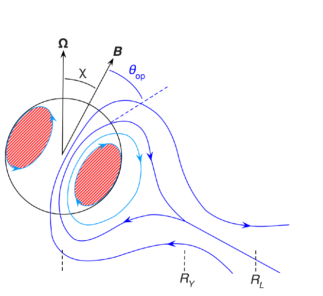
Figure 1: Interior and exterior field of a newborn magnetar. Poloidal-field lines are shown in blue; the internal toroidal field (directed perpendicular to the page) is located in the red shaded region. The exterior field geometry and the star’s spindown depend on the rotation and magnetic-field strength. The open-field line region of the magnetosphere, with opening half-angle $\theta_{\rm op}$, begins at a line joining to an equatorial current sheet at the $Y$-point, located at a radius $R_{Y}$ from $\boldsymbol{\Omega}$. Both $R_{Y}$ and the Alfvén radius $R_{A}$ evolve in time towards the light-cylinder radius $R_{L}$, with $R_{Y}\leq R_{A}\leq R_{L}$.

The environment around a NS determines how rapidly it loses angular momentum, and hence spins down. This occurs even if the exterior region is vacuum, through Poynting-flux losses at a rate (proportional to $\sin^{2}\chi$) which may be solved analytically (Deutsch, 1955). The vacuum-exterior assumption is still fairly frequently employed in the pulsar observational literature, although it exhibits the pathological behaviour that spin-down decreases as $\chi\to 0^{\circ}$ and ceases altogether for an aligned rotator ($\chi=0^{\circ}$).

The magnetic-field structure outside a NS, and the associated angular-momentum losses, change when one accounts for the distribution of charged particles that will naturally come to populate the exterior of a pulsar (Goldreich & Julian, 1969). Solving for the magnetospheric structure is now analytically intractable, but numerical force-free solutions for the cases of $\chi=0^{\circ}$ (Contopoulos et al., 1999) and $\chi\neq 0^{\circ}$ (Spitkovsky, 2006) demonstrate a structure similar to that sketched in Fig. 1: one region of closed, corotating equatorial field lines and another region of ‘open’ field lines around the polar cap. The two are delineated by a separatrix: a cusped field line that joins an equatorial current sheet at the $Y$-point $R_{Y}$. Corotation of particles along magnetic fields ceases to be possible if their linear velocity exceeds the speed of light; this sets the light cylinder radius $R_{L}=c/\Omega$. In practice, simulations employing force-free electrodynamics find magnetospheric structures with $R_{Y}=R_{L}$, although solutions with $R_{Y}<R_{L}$ are not, a priori, inadmissible. The angular-momentum losses from these models proved to be non-zero in the case $\chi=0^{\circ}$, in contrast with the vacuum-exterior case. These losses again correspond to the radiation of Poynting flux, but are enhanced compared with the vacuum case, since there is now additional work done on the charge distribution outside the star (Timokhin, 2006). Results from these simulations should be applicable in the ultrarelativistic wind limit, and since it appears $R_{Y}=R_{L}$ generically for this case, the losses are also independent of any details of the magnetospheric structure.

Shortly after birth, however, a magnetar exterior is unlikely to bear close resemblance to the standard pulsar-magnetosphere models. A strong neutrino-heated wind of charged particles will carry angular momentum away from the star (Thompson et al., 2004) – a concept familiar from the study of non-degenerate stars (Schatzman, 1962) – and these losses may dominate over those of Poynting-flux type. At large distances from the star, a particle carries away more angular momentum than if it were decoupled from the star at the stellar surface. At sufficient distance, however, there will be no additional enhancement to angular momentum losses as the particle moves further out; the wind speed exceeds the Alfvén speed, meaning the particle cannot be kept in corotation with the star. The radius at which the two speeds become equal is the Alfvén radius $R_{A}$.

An additional physical mechanism for angular-momentum loss becomes important at rapid rotation: as well as thermal pressure, a centrifugal force term assists in driving the particle wind. Each escaping particle then carries away an enhanced amount of angular momentum (Mestel, 1968a; Mestel & Spruit, 1987). The mechanism is active up to the sonic radius $R_{s}=(GM/\Omega^{2})^{1/3}$, at which these centrifugal forces are strong enough to eject the particle from its orbit. If it is still in corotation with the star until the point when it is centrifugally ejected, i.e. $R_{A}\geq R_{s}$, the maximal amount of angular momentum is lost.

Another source of angular-momentum losses is plausible in the aftermath of the supernova creating the magnetar: a magnetic torque from the interaction of the stellar magnetosphere with fallback material. The physics of this should resemble that of the classic problem of a magnetic star with an accretion disc (Ghosh & Lamb, 1978), but the dynamical aftermath of the supernova is far messier, and results will be highly sensitive to the exact physical conditions of the system. Attempting to account for fallback matter would therefore not make our model any more quantitatively accurate.

We recall that there are four radii of importance in the magnetar-wind problem. Two of them, $R_{L}$ and $R_{s}$, depend only on the stellar rotation rate. The others are $R_{Y}$, associated with electromagnetic losses, and $R_{A}$, associated with particle losses. We will need to account for how these quantities, which both grow until reaching $R_{L}$, evolve over the early phase of the magnetar’s life. Finally, we also need to know, at a given instant, the dominant physics governing the star’s angular-momentum loss. This is captured in the wind magnetisation $\sigma_{0}$, the ratio of Poynting-flux to particle kinetic energy losses:

$$\sigma_{0}=\frac{B_{\rm ext}^{2}\mathcal{F}_{\rm op}^{2}R_{*}^{4}\Omega^{2}}{\dot{M}c^{3}},$$ (2)

where $\mathcal{F}_{\rm op}$ is the fraction of field lines which remain open beyond $R_{Y}$ (see Fig. 1) and $B_{\rm ext}$ is the surface field strength. Note that the limits $\sigma_{0}\ll 1$ ($\sigma_{0}\gg 1$) correspond to non(ultra)-relativistic winds.

At present there are neither analytic nor numerical solutions providing a full description of the proto-magnetar wind. In the absence of these, we will adapt the model of Metzger et al. (2011) (hereafter M11), which at least attempts to incorporate, semi-quantitatively, the main ingredients that such a full wind solution should have. Based on their work, we have devised a simplified semi-analytic model for the magnetar wind, capturing the same fundamental wind physics but more readily usable for our simulations. Our description of the details is brief, but self-contained if earlier results are taken on trust; we denote some equation X taken from M11 by (M11;X).

To avoid cluttering what follows with mass and radius factors, we report equations and results for our fiducial magnetar model with $R_{*}=12$ km and a mass $1.4M_{\odot}$. We have, however, performed simulations with a $15$-km radius, $2.4M_{\odot}$ model, as a crude approximation to a massive magnetar formed through binary inspiral (Giacomazzo & Perna, 2013), finding similar results.

We start from the established mass-loss rate $\dot{M}_{\nu}$ (Qian & Woosley, 1996) of a non-rotating, unmagnetised proto-NS:

$$\dot{M}_{\nu}=-6.8\times 10^{-5}M_{\odot}\textrm{s}^{-1}\!\left({\!\frac{L_{\nu}}{10^{52}\textrm{erg s}^{-1}}\!}\right)^{\!5/3}\!\left({\!\frac{E_{\nu}}{10\textrm{ MeV}}\!}\right)^{\!10/3},$$ (3)

where $M_{\odot}$ is the solar mass and $L_{\nu}$ and $E_{\nu}$ are the neutrino luminosity and energy per neutrino, respectively. The idea will be to adjust this result to account for the effects of rotation and a magnetic field. From the simulations of Pons et al. (1999) (see M11 Fig. A1), we make the following fits to the evolution of $L_{\nu}$ and $E_{\nu}$:

$$\frac{L_{\nu}}{10^{52}\textrm{ erg s}^{-1}} \approx 0.7\exp\left({-\frac{t\textrm{ [s]}}{1.5}}\right)+0.3\left({1-\frac{t\textrm{ [s]}}{50}}\right)^{4}\ ,$$

$$\frac{E_{\nu}}{10\textrm{ MeV}} \approx 0.3\exp\left({-\frac{t\textrm{ [s]}}{4}}\right)+1-\frac{t\textrm{ [s]}}{60}\ .$$ (4)

Our model does not allow for evolution of the radius $R_{*}$, so our time zero corresponds to two seconds after bounce, at which point $R_{*}$ has stabilised at $\sim 12$ km.

Charged particles can only escape the magnetised star along the fraction of open field lines, so the original mass-loss rate (3) should be reduced to $\dot{M}=\dot{M}_{\nu}\mathcal{F}_{\rm op}$, where (M11;A4)

$$\mathcal{F}_{\rm op}=1-\cos(\theta_{\rm op})=1-\cos\left[\arcsin\left({\sqrt{R_{*}/R_{Y}}}\right)\right].$$ (5)

Now since $\cos(\arcsin x)=\sqrt{1-x^{2}}$, we have

$$\mathcal{F}_{\rm op}=1-\sqrt{1-R_{*}\mathfrak{R}_{LY}/R_{L}},$$ (6)

where $\mathfrak{R}_{LY}\equiv R_{L}/R_{Y}$. When $f\gtrsim 500$ Hz, the mass loss may experience a centrifugal enhancement $\mathcal{F}_{\rm cent}>1$, so that (M11;A15):

$$\dot{M}=\dot{M}_{\nu}\mathcal{F}_{\rm op}\mathcal{F}_{\rm cent}.$$ (7)

Our approach will be first to ignore this to obtain a slow-rotation solution, which we then use to calculate $\mathcal{F}_{\rm cent}$ (and hence the general $\dot{M}$) ‘perturbatively’. We start by combining equations (6) and (2) (with $\mathcal{F}_{\rm cent}=1$) to get a relation between $\mathfrak{R}_{LY}$ and $\sigma_{0}$. But another, phenomenological relation $\mathfrak{R}_{LY}=\max\{(0.3\sigma_{0}^{0.15})^{-1},1\}$ (Bucciantini et al., 2006; Metzger et al., 2007) also links the two. The relations may therefore be combined to eliminate $\sigma_{0}$:

$$\left({1-\sqrt{1-\frac{R_{*}}{R_{L}}\mathfrak{R}_{LY}}}\right)\mathfrak{R}_{LY}^{1/0.15}=\frac{0.3^{-1/0.15}c^{3}\dot{M}_{\nu}}{B_{\rm ext}^{2}R_{*}^{4}\Omega^{2}}.$$ (8)

This equation may be solved to find $\mathfrak{R}_{LY}$ for given $B_{\rm ext},\Omega$ and $t$. It has real solutions as long as $R_{*}/R_{Y}<1$; the $Y$-point cannot be within the star. As $R_{Y}\to R_{*}$ all magnetospheric field lines become open, and the following limits are attained:

$$\mathfrak{R}_{LY}=R_{L}/R_{*}\ ,\ \mathcal{F}_{\rm op}=1\ ,\ \sigma_{0}=B_{\rm ext}^{2}R_{*}^{4}\Omega^{2}/(\dot{M}_{\nu}c^{3}).$$ (9)

Accordingly, in cases where equation (8) has no real solutions, we use the above limiting values.

Figure 2: The first 80 s of rotational evolution for different model newborn magnetars, with fixed $\chi$ and (from left to right): $f_{0}=1$ kHz, $B_{\rm ext}=10^{16}$ G; $f_{0}=100$ Hz, $B_{\rm ext}=10^{16}$ G; $f_{0}=1$ kHz, $B_{\rm ext}=10^{15}$ G. Linestyles 1,2 show (respectively) $\chi=0,90^{\circ}$ models evolved with the magnetar wind prescription described in section 2.2 for 40 s and thereafter with a ‘pulsar’ prescription (third line of equation (12)); linestyles 3,4 show the corresponding results using the ‘pulsar’ prescription from birth. Note that before 40 s, lines 1 and 2 become indistinguishable from one another for higher $f_{0}$ and $B_{\rm ext}$.

Next we move on to calculate the centrifugal enhancement. As discussed earlier, this depends strongly on the location of $R_{A}$ with respect to $R_{s}$. Only the former quantity depends on the magnetospheric physics, and as for the $Y$-point location we find it convenient to work with the dimensionless radius $\mathfrak{R}_{LA}\equiv R_{L}/R_{A}$. Now, M11 employ the phenomenological relation $\mathfrak{R}_{LA}=\max\{\sigma_{0}^{-1/3},1\}$; we therefore just need to find $\sigma_{0}$. To do so, we use the solution we have just obtained for $\mathfrak{R}_{LY}$, plugging it in equation (7) to make a first calculation of $\dot{M}$ in the absence of any centrifugal enhancement (i.e. setting $\mathcal{F}_{\rm cent}=1$), then using the result in equation (2) to find $\sigma_{0}$. We may now calculate the centrifugal enhancement:

$$\mathcal{F}_{\rm cent}=\mathcal{F}_{\rm cent}^{\rm max}[1-\exp(-R_{A}/R_{s})]+\exp(-R_{A}/R_{s}),$$ (10)

where (M11;A12,A13)

$$\mathcal{F}_{\rm cent}^{\rm max}=\exp\left[\left({\frac{f[\textrm{kHz}]}{2.8\max\{\sin(\theta_{\rm op}),\sin\chi\}}}\right)^{1.5}\right]$$ (11)

is the maximum possible enhancement factor to the mass loss, occurring when $R_{A}\geq R_{s}$.

The centrifugal enhancement relies on particles reaching large distances from $\boldsymbol{\Omega}$ whilst remaining in corotation; we can see this will not happen if open field lines remain close to this axis out to large distances. As a diagnostic of this, M11 assume that enhancement will not occur if a typical open-field line angle $(\chi+\theta_{\rm op})\ll\pi/2$, but will do if $(\chi+\theta_{\rm op})\gtrsim\pi/2$. In practice we have to decide on an angle delineating the two regimes: we take $\pi/4$. Accordingly, we will adopt equation (7) for the full mass-loss rate, but set $\mathcal{F}_{\rm cent}=1$ when $\chi+\theta_{\rm op}<\pi/4$. We now re-calculate equation (2) to find the full $\sigma_{0}$, and so the EM energy-loss rate (M11;A5):

$$\dot{E}_{\rm EM}=\begin{cases}c^{2}\dot{M}\sigma_{0}^{2/3}&\sigma_{0}<1\textrm{ and }t<40\textrm{s}\\ \frac{2}{3}c^{2}\dot{M}\sigma_{0}&\sigma_{0}\geq 1\textrm{ and }t<40\textrm{s}\\ -\frac{R_{*}^{2}}{4c^{3}}\Omega^{4}B_{\rm ext}^{2}(1+\sin^{2}\chi)&t\geq 40\textrm{s}.\end{cases}$$ (12)

Within one minute, the bulk of the star’s neutrinos have escaped and so the proto-magnetar wind weakens greatly. Here we take the wind to be negligible after $40$ s, at which point we switch to a fit (Spitkovsky, 2006) to numerical simulations of pulsar magnetospheres, corresponding to the ultrarelativistic limit of the wind (i.e. kinetic losses being negligible). For all our models $\sigma_{0}$ becomes large and $R_{Y}\to R_{L}$ before the $40$-second mark at which we switch to this regime; see M11 for more details.

Note that the first and second lines of equation (12) are formally correct only in the limits $\sigma_{0}\ll 1$ and $\sigma_{0}\gg 1$, respectively, with no such simple expressions existing for the case $\sigma_{0}\sim 1$. Treating the latter case is beyond the scope of the present work, so we simply switch between the first two regimes of equation (12) at $\sigma_{0}=1$. We do not expect this to introduce any serious uncertainty in our work, however: the wind magnetisation makes a rapid transition between the two limiting regimes over a timescale short compared with the evolution of both $\chi$ and $\Omega$.

Fig. 2 shows sample evolutions, comparing the magnetar wind prescription with one often used for pulsars (and also used, with a slightly different numerical prefactor, in Lander & Jones (2018)). For the extreme case of $f_{0}=1$ kHz, $B_{\rm ext}=10^{16}$ G (left-hand panel), we see that the rotation rate has roughly halved after 40 s for all models – although the most rapid losses are suffered by the model with $\chi=90^{\circ}$ and the pulsar prescription. For less extreme cases (middle and right panels), however, the magnetar wind always gives the greatest losses. Finally, as expected from equation (12), we see that the value of $\chi$ often has less effect on the magnetar-wind losses than those from the pulsar prescription.

2.3 Buoyancy forces

At a much later stage, another physical effect needs to be modelled, related to the role of buoyancy forces on internal motions.

The proportions of different particles in a NS varies with depth. If one moves an element of NS matter to a different depth, chemical reactions act to re-equilibrate it with its surroundings, on a timescale $\tau_{\rm chem}$. When the temperature $T$ is high, $\tau_{\rm chem}\ll P_{\rm prec}$, so moving fluid elements are kept in chemical equilibrium. Once the star has cooled sufficiently, however, reactions will have slowed down enough for fluid elements to retain a different composition from their surroundings (Lander & Jones, 2018); they will therefore be subject to a buoyancy force due to the chemical gradient (Reisenegger & Goldreich, 1992). This force tends to suppress radial motion, and hence will predominantly affect the compressible piece of the motions (Mestel & Takhar, 1972; Lasky & Glampedakis, 2016). For this phase, one would ideally generalise the lengthy calculation of Lander & Jones (2017) to include buoyancy forces, but this is very likely to be intractable. In lieu of this, we will simply impose that the motions become divergence-free below some temperature $T_{\rm solen}$, which we define to be the temperature for which

$$P_{\rm prec}=\tau_{\rm chem}=0.2\left({\frac{T}{10^{9}\textrm{ K}}}\right)^{-6}\left({\frac{\bar{\rho}}{\rho_{\rm nuc}}}\right)^{2/3},$$ (13)

taking the expression for $\tau_{\rm chem}$ from Reisenegger & Goldreich (1992), and where $\rho_{\rm nuc}$ is nuclear density and $\bar{\rho}$ the average core density. $T_{\rm solen}$ is clearly a function of $B_{\rm int}$ and $\Omega$; its typical value is $10^{9}-10^{10}$ K. For $T<T_{\rm solen}$, bulk viscous dissipation (depending on the compressibility of the internal motions) therefore becomes redundant, and we shut it off in our evolutions, leaving only the ineffective shear-viscous dissipation. Without significant viscous damping, the star’s proclivity towards becoming an orthogonal rotator ($\chi=90^{\circ}$) is suppressed.

Our evolutionary model employs standard fluid physics, and cannot therefore describe any effects related to the gradual formation of the star’s crust. The star’s motion depends on distortions misaligned from the rotation axis; at late stages this may include, or even be dominated by, elastic stresses in the crust. For the magnetar-strength fields we consider, however, it is reasonable to assume that magnetic distortions dominate. Our fluid model of a magnetar’s $\chi$-evolution should predict the correct long-timescale trend, even if it cannot describe short-timescale seismic features (see discussion).

Finally, as the star cools the core will form superfluid components, and the interaction between these may provide a new coupling mechanism between the rotation and magnetic-field evolution (Ruderman et al., 1998). It is not clear what effect – if any – this will have on the long-timescale evolution of $\chi$.

3 Evolution equations

We follow the coupled $\Omega-\chi$ evolution of a newborn magnetar with a strong, large-scale toroidal $B_{\rm int}$ in its core – the expected outcome of the birth physics (Jones, 1976; Thompson & Duncan, 1993). For stability reasons (Tayler, 1980) this must be accompanied by a poloidal-field component, but we will assume that within the star it is small enough to be ignored here (it also retains consistency with the solution we have for the internal motions; Lander & Jones (2017)). We assume there is no internal motion, and hence no dissipation, in the outer envelope (the region that becomes the crust once the star has cooled sufficiently).

One unrealistic feature of purely toroidal fields is that $B_{\rm ext}=0$. As in Lander & Jones (2018), we will assume that the poloidal-field component – negligible within the star – becomes significant as one moves further out, and links to a substantial $B_{\rm ext}$ sharing the same symmetry axis as $B_{\rm int}$. We then express the magnetic ellipticity as:

$$\epsilon_{B}=-3\times 10^{-4}\left({\frac{B_{\rm int}}{10^{16}\textrm{ G}}}\right)^{2}=-3\times 10^{-4}\left({\frac{B_{\rm int}}{B_{\rm ext}}}\right)^{2}\left({\frac{B_{\rm ext}}{10^{16}\textrm{ G}}}\right)^{2},$$ (14)

where the first equality comes from self-consistent solutions of the star’s hydromagnetic equilibrium (Lander & Jones, 2009) with a purely toroidal internal field, and the second equality links this ellipticity to the exterior field strength (somewhat arbitrarily) through the ratio $B_{\rm ext}/B_{\rm int}$. Note that the negative sign of $\epsilon_{B}$ indicates that the distortion is prolate.

A typical model encountered in the literature (e.g. Stella et al. (2005)) assumes a ‘buried’ magnetic field, with $B_{\rm ext}/B_{\rm int}\ll 1$, although self-consistent equilibrium models with vacuum exteriors have $B_{\rm ext}\sim B_{\rm int}$ (Lander & Jones, 2009). The results for $f$ and $\chi$ vary little with the choice of this ratio, since it is mostly the exterior torque, i.e. $B_{\rm ext}$, that dictates the last-phase evolution, and we therefore set the ratio to unity for simplicity unless stated otherwise – an upper limit for our model, as $B_{\rm ext}/B_{\rm int}\gtrsim 1$ would be inconsistent with the toroidal field dominating within the star. Only in section 6 do we explore varying this ratio, as the predicted gravitational and electromagnetic emission are affected by the relative strength of the magnetic field inside and outside the star.

The $\Omega$-evolution is given by the simple, familiar expression:

$$\dot{\Omega}=\frac{\dot{E}_{\rm EM}}{I\Omega},$$ (15)

where $I$ is the moment of inertia, whilst the $\chi$-evolution involves an interplay between viscous dissipation $\dot{E}_{\rm visc}$ of internal fluid motions, and external torques:

$$\dot{\chi}=\frac{\dot{E}_{\rm visc}}{I\epsilon_{B}\sin\chi\cos\chi\Omega^{2}}+\frac{\dot{E}_{\rm EM}^{(\chi)}}{I\Omega^{2}}.$$ (16)

Now, $\dot{\chi}$ should vanish for $\chi=0^{\circ},90^{\circ}$ (Mestel, 1968b). The $\dot{E}_{\rm EM}$ from equation (12) does not satisfy this, however; it represents the spindown part of the full external torque, whereas $\dot{\chi}$ depends on a torque component orthogonal to this. As a simple fix that gives the correct limiting behaviour of $\dot{\chi}$, we take $\dot{E}_{\rm EM}^{(\chi)}=\sin\chi\cos\chi\dot{E}_{\rm EM}$ for $t<40$ s. For the later phase, Philippov et al. (2014) suggest the expression

$$\dot{E}_{\rm EM}^{(\chi)}=\frac{R_{*}^{2}}{4c^{3}}\Omega^{4}B_{\rm ext}^{2}k\sin\chi\cos\chi,$$ (17)

based on fits to numerical simulations, and finding $k\approx 1$ for dipolar pulsar magnetospheres. This is a sensible result, since setting $k=1$ in equation (17) gives the analytic result for the case of a vacuum exterior. Evolutions for a vacuum exterior were performed in Lander & Jones (2018); we also considered pulsar-like models, but with an alignment torque that did not vanish as $\chi\to 0^{\circ}$. The present treatment improves upon this.

Although equation (17) reflects the physics of pulsar magnetospheres, the coronae of magnetars have a different physical origin and are likely to be complex multipolar structures, which will in turn affect the alignment torque. Furthermore, there are hints that a magnetar corona may lead to an enhanced torque, $k>1$, compared with the pulsar case (Thompson et al., 2002; Younes et al., 2017). On the other hand, for relatively modest magnetic fields ($B\sim 10^{14}$ G) these coronae are likely to be transient features (Beloborodov & Thompson, 2007; Lander, 2016); whilst we may still think of $k$ as embodying the long-term average torque, it therefore seems implausible for the appropriate value of $k$ to be far larger than unity. In the absence of suitable quantitative results for magnetars, here we will simply adopt equation (17) to describe the alignment, but explore varying the torque prefactor $k$ to check how strong the alignment torque needs to be for consistency with the model.

Finally, the gravitational radiation reaction torque on the star – like its electromagnetic counterpart – has an aligning effect on the ${\boldsymbol{B}}$ and $\boldsymbol{\Omega}$ axes. It is given by a straightforward expression that could be included in our evolutions; we neglect it, however, as one can easily show that the GW energy losses (Cutler & Jones, 2001) in (15) and (16) are always negligible compared with $\dot{E}_{\rm EM}$ for the models we consider. For instance, for a star with $B_{\rm ext}=10^{16}$ G and $f=1$ kHz, the ratio of GW-driven spindown to EM Poynting-type spindown is $\sim 10^{-4}$. This ratio scales as $f^{2}B_{\rm int}^{4}/B_{\rm ext}^{2}$, so would be even smaller for more slowly spinning and less strongly magnetised stars. Furthermore, we have not considered the torque enhancement due to the magnetar wind, which would further reduce the ratio.

Viscosity coefficients have strong $T$-dependence, so this should also be accounted for. We assume an isothermal stellar core (recall that we do not consider dissipation in the envelope/crust) with

$$\frac{T(t)}{10^{10}\textrm{ K}}=\begin{cases}40-\frac{39}{40}t[\textrm{s}]&t\leq 40\textrm{ s},\\ [1+0.06(t[\textrm{s}]-40)]^{-1/6}&t>40\textrm{ s},\end{cases}$$ (18)

which mimics the differing cooling behaviour in the neutrino diffusion and free-streaming regimes, with the latter expression coming from Page et al. (2006). The isothermal assumption is indeed quite reasonable for the latter case, though less so for the former (see, e.g., Pons et al. (1999)); the temperature may vary by a factor of a few in the core at very early times.

In calculating the viscous energy losses $\dot{E}_{\rm visc}$ we assume the same well known forms for shear and bulk viscosity as described in Lander & Jones (2018). Whilst shear viscosity is always assumed to be active (albeit inefficient), bulk viscosity is not. We have already discussed why we take it to be inactive at late times when $T<T_{\rm solen}$, but it is also suppressed in the early era, whilst the proto-neutron star matter is still partially neutrino-opaque and reactions are inhibited. Following Lai (2001), we will switch on bulk viscosity once the temperature drops below $3\times 10^{10}$ K. Note that while we include the viscosity mechanisms traditionally considered in such analyses as ours, other mechanisms can act. Of possible relevance in the very early life of our star is the shear viscosity contributed by the neutrinos themselves (see e.g. Guilet et al. (2015)). We leave study of this to future work, merely noting for now that its inclusion would increase the tendency for our stars to orthogonalise.

Whatever its microphysical nature, viscous dissipation acts on the star’s internal fluid motions, for which we use the only self-consistent solutions to date (Lander & Jones, 2017). We do not allow for any evolution of $B_{\rm int}$.

4 Simulations

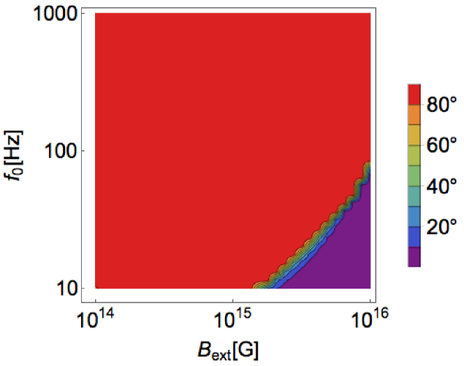
Figure 3: Distribution of inclination angles (colourscale) after one day, for a range of $f_{0}$ and $B_{\rm ext}$ as shown, and with $\chi_{0}=1^{\circ}$ for all models. All models in the considered parameter range have already reached either the aligned- or orthogonal-rotator limit, though the orthogonal rotators will all start to align at later times.

We solve the coupled $\Omega-\chi$ equations (15) and (16) with the physical input discussed above. The highly coupled and non-linear nature of the equations means that numerical methods are required, and we therefore use adapted versions of the Mathematica notebooks described in detail in Lander & Jones (2018). Only in a few limits are analytic results possible, e.g. at late times where $\chi$ has reduced to nearly zero (see below), and the spin-down then proceeds as the familiar power-law solution to equation (12). Unless stated otherwise, we start all simulations with a small initial inclination angle, $\chi_{0}\equiv\chi(t=0)=1^{\circ}$.

Fig. 3 shows the distribution of $\chi$ after one day, for our chosen newborn-magnetar parameter space $f_{0}\equiv f(t=0)=10-10^{3}\textrm{ Hz},\ B_{\rm ext}=10^{14}-10^{16}\textrm{ G}$ and with $k=2$. This is similar to our earlier results (Lander & Jones, 2018), where the effect of buoyancy forces on interior motions was not considered. As the orthogonalising effect of internal viscosity becomes suppressed, the orthogonal rotators can be expected to start aligning at later times, whilst the small region of aligned rotators will obviously remain with $\chi\approx 0^{\circ}$. If rapid rotation drives magnetic-field amplification, however, a real magnetar born with such a low $f$ could not reach $B\sim 10^{16}$ G.

Figure 4: Evolution of $f$ (solid line) and $\chi$ (dashed line) for two magnetars. Top: $f_{0}=1$ kHz, $B_{\rm int}=B_{\rm ext}=10^{16}$ G, bottom: $f_{0}=100$ Hz, $B_{\rm int}=B_{\rm ext}=10^{14}$ G. For illustrative purposes $\chi_{0}=30^{\circ}$ is chosen, but a smaller value is more likely. For both models $\chi$ decreases for the first $\sim 40$ s, then increases rapidly to $90^{\circ}$ as bulk viscosity becomes active, staying there until the internal motions become solenoidal (at $t\sim 10^{3}$ s for the left-hand model; at $t\sim 10^{8}$ s for the right-hand one), after which the spindown torque is able, slowly, to drive $\chi$ back towards $0^{\circ}$.

Fig. 4 shows the way $f$ and $\chi$ evolve, for all models in our parameter space except the aligned rotators of Fig. 3: an early phase of axis alignment, rapid orthogonalisation, then slow re-alignment. The evolution for most stars in our considered parameter range is similar, though proceeds more slowly for lower $B_{\rm int}$, $B_{\rm ext}$ and $f_{0}$, as seen by comparing the left- and right-hand panels (see also Fig. 5 and 6).

Figure 5: Distribution of spin periods (colourscale) for magnetars with the shown range of $B_{\rm ext}$ and $f_{0}$ at ages of $1000$ yr (left) and $5000$ yr (right). For all models $\chi_{0}=1^{\circ}$ and $B_{\rm int}=B_{\rm ext}$.

5 Comparison with observations

Next we compare our model predictions with the population of observed magnetars. Typical magnetars have $P\sim 2-12$ s and $B_{\rm ext}\sim 10^{14}-10^{15}$ G; comparing these values with Fig. 5, we see that they are consistent with the expected ages of magnetars, roughly $1000-5000$ yr (see, e.g., Tendulkar et al. (2012)). The results in Fig. 5 are virtually insensitive to the exact value of the alignment-torque prefactor $k$ (we take $k=2$ in these plots). The model results are very similar for different $B_{\rm int}$ and $\chi_{0}$, and the vertical contours show that present-day periods are set primarily by $B_{\rm ext}$, and give no indication of the birth rotation.

Observations contain more information than just $P$ and the inferred $B_{\rm ext}$, however. The four magnetars observed in radio (Olausen & Kaspi, 2014):

name	$P$/s	$B_{\rm ext}/(10^{14}\textrm{ G})$
1E 1547.0-5408	2.1	3.2
PSR J1622-4950	4.3	2.7
SGR J1745-2900	3.8	2.3
XTE J1810-197	5.5	2.1

are particularly interesting. They have in common a flat spectrum and highly-polarised radio emission that suggests they may all have a similar exterior geometry, with $\chi\lesssim 30^{\circ}$ (Kramer et al., 2007; Camilo et al., 2007, 2008; Levin et al., 2012; Shannon & Johnston, 2013). The probability of all four radio magnetars having $\chi<30^{\circ}$, assuming a random distribution of magnetic axes relative to spin axes, is $(1-\cos 30^{\circ})^{4}\approx 3\times 10^{-4}$, indicating that such a distribution is unlikely to happen by chance. Low values of $\chi$ could explain the paucity of observed radio magnetars: if the emission is from the polar-cap region, it would only be seen from a very favourable viewing geometry. Beyond the four radio sources, modelling of magnetar hard X-ray spectra also points to small $\chi$ (Beloborodov, 2013; Hascoët et al., 2014), giving further weight to the idea that small values of $\chi$ are generic for magnetars.

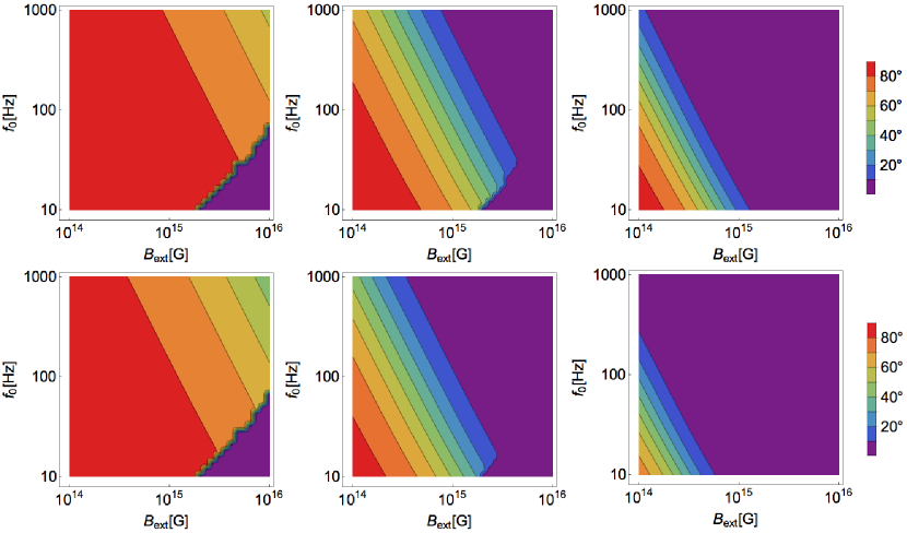
Figure 6: Distribution of $\chi$ (colourscale) for magnetars with an alignment torque prefactor of (from left to right) $k=1,2$ and $3$; and at ages of $1000$ yr (top panels) and $5000$ yr (bottom panels). As before, $\chi_{0}=1^{\circ}$ and $B_{\rm int}=B_{\rm ext}$ for all models.

Now comparing with Fig. 6, we see that – by contrast with the present-day $P$ – the present-day $\chi$ does encode interesting information about magnetar birth. Unfortunately, as noted by Philippov et al. (2014), the results are quite sensitive to the alignment-torque prefactor $k$. We are also hindered by the dearth of reliable age estimates for magnetars. Nonetheless, we will still be able to draw some quite firm conclusions, and along the way constrain the value of $k$.

Let us assume a fiducial mature magnetar with $\chi<30^{\circ}$, $B_{\rm ext}=3\times 10^{14}$ G (i.e. roughly halfway between $10^{14}$ and $10^{15}$ G on a logarithmic scale) and a strong internal toroidal field (so that it will have had $\chi\approx 90^{\circ}$ at early times). We first observe that such a star is completely inconsistent with $k=1$ unless it is far older than $5000$ yr, so we regard this as a strong lower limit.

If $k=2$, Fig. 6 shows us that the birth rotation must satisfy $f_{0}\gtrsim 1000$ Hz if our fiducial magnetar is $1000$ yr old, or $f_{0}\gtrsim 300$ Hz for a $5000$-yr-old magnetar. The former value may just be possible, in that the break-up rotation rate is typically over 1 kHz for any reasonable neutron-star equation of state – but is clearly extremely high. The latter value of $f_{0}$ is more believable, but does require the star to be towards the upper end of the expected magnetar age range.

Finally, if $k=3$ the birth rotation is essentially unrestricted: it implies $f_{0}\gtrsim 20-100$ Hz for the age range $1000-5000$ yr. As discussed earlier, however, this represents a very large enhancement to the torque – with crustal motions continually regenerating the magnetar’s corona – and sustaining this over a magnetar lifetime (especially $5000$ yr) therefore seems very improbable.

An accurate value of $k$ (or at least, its long-term average) cannot be determined without more detailed work, so we have to rely on the qualitative arguments above. From these, we tentatively suggest that existing magnetar observations indicate that $f_{0}\gtrsim 100-300$ Hz and $2\lesssim k<3$ for these stars. Furthermore, from Fig. 6, we see that a single measurement of $\chi\gtrsim 15^{\circ}$ from one of the more highly-magnetised (i.e. $B_{\rm ext}\sim 10^{15}$ G) observed magnetars would essentially rule out $k\geq 3$.

6 Gravitational and electromagnetic radiation

6.1 GWs from newborn magnetars

An evolution $\chi\to 90^{\circ}$ brings a NS into an optimal geometry for GW emission (Cutler, 2002), and a few authors have previously considered this scenario applied to newborn magnetars (Stella et al., 2005; Dall’Osso et al., 2009), albeit without the crucial effects of the protomagnetar wind and self-consistent solutions for the internal motions. By contrast, we have these ingredients, and hence can calculate GWs from newborn magnetars more quantitatively. In Fig. 7 we plot the characteristic GW strain at distance $d$:

$$h_{\rm c}(t)=\frac{8G}{5c^{4}}\frac{\epsilon_{B}I\Omega(t)^{2}\sin^{2}\chi(t)}{d}\left({\frac{f_{\rm GW}^{2}}{|\dot{f}_{\rm GW}|}}\right)^{1/2}$$ (19)

from four model magnetars with $\chi_{0}=1^{\circ}$, averaged over sky location and source orientation, following Jaranowski et al. (1998). This signal is emitted at frequency $f_{\rm GW}=2f=\Omega/\pi$. We also show the design rms noise $h_{\rm rms}=\sqrt{f_{\rm GW}S_{h}(f_{\rm GW})}$ for the detectors aLIGO (Abbott et al., 2018) and ET-B (Hild et al., 2008), where $S_{h}$ is the detector’s one-sided power spectral density. Models 1 and 2 from Fig. 7 both have $f_{0}=1000$ Hz and $B_{\rm int}=10^{16}$ G, but the former model has a much stronger exterior field. As a result, it is subject to a strong wind torque, which spins it down greatly before $\chi\to 90^{\circ}$, thus reducing its GW signal compared with model 2.

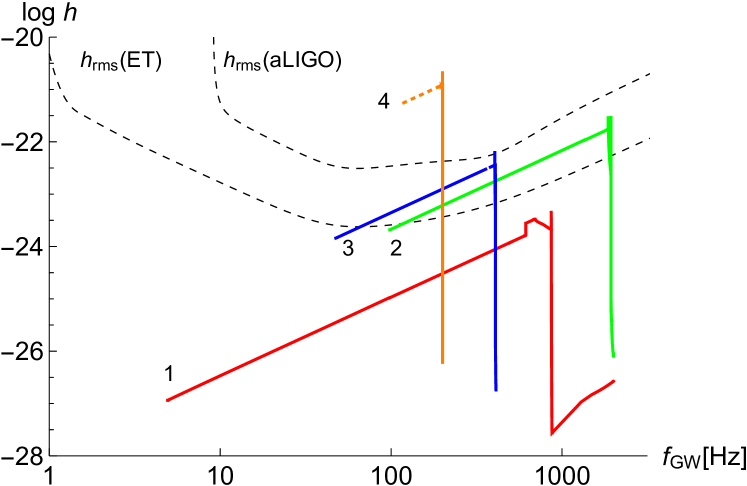
Figure 7: GW signal $h_{\rm c}$ from four model newborn magnetars, against the noise curves $h_{\rm rms}$ for aLIGO and ET. Three models are for one week of signal at $d=20$ Mpc (i.e. Virgo galaxy cluster): (1) $f_{0}=1$ kHz, $B_{\rm ext}=B_{\rm int}=10^{16}$ G, (2) $f_{0}=1$ kHz, $B_{\rm ext}=0.05B_{\rm int}=5\times 10^{14}$ G, (3) $f_{0}=200$ Hz, $B_{\rm ext}=0.05B_{\rm int}=10^{15}$ G; and the final signal (4) is at $d=10$ kpc (i.e. in our galaxy) and has duration of one year (solid line for the first week, dotted for the rest), with $B_{\rm ext}=0.05B_{\rm int}=5\times 10^{13}$ G, $f_{0}=100$ Hz.

Next we calculate the signal-to-noise ratio (SNR) for our selected models, following Jaranowski et al. (1998):

$$\textrm{SNR}=\left[\int\limits_{t=0}^{t_{\rm final}}\left({\frac{h_{\rm c}}{h_{\rm rms}}}\right)^{2}\frac{|\dot{f}_{\rm GW}|}{f_{\rm GW}}\ \mathrm{d}t\right]^{1/2}.$$ (20)

Note that this expression assumes single coherent integrations. In reality it will be difficult to track the evolving frequency well enough to perform such integrations; see discussion in Section 7.

Using aLIGO, models 1, 2, 3 and 4 have $\textrm{SNR}=0.018,0.38,0.43,4.0$ for $t_{\rm final}=1$ week. With ET, we find SNR values of $0.19,4.5,4.4,47$ for models 1, 2, 3, 4, again taking $t_{\rm final}=1$ week. Model 4 would be detectable for longer; taking instead $t_{\rm final}=1$ yr gives $\textrm{SNR}=16$ ($200$) for aLIGO (ET). Once $\chi$ for this model reduces below $90^{\circ}$, the GW signal will gain a second harmonic at $f$, in addition to the one at $2f$ (Jones & Andersson, 2002) . However, even after $150$ yr (when the model-4 signal drops below the ET noise curve), the star is still an almost-orthogonal rotator, with $\chi=81^{\circ}$. In this paper, therefore, it is enough to consider only the $2f$ harmonic.

Recently, Dall’Osso et al. (2018) studied GWs from newborn magnetars, finding substantial SNR values even using aLIGO. To compare with them, we take one of their $\textrm{SNR}=5$ models, which has $B_{\rm ext}/B_{\rm int}=0.019$ and $f_{0}=830$ Hz. From their equations (25) and (26), however, they appear to have a different numerical prefactor from ours; if this was used in their calculations their SNR values should be multiplied by $\sqrt{2/5}$ for direct comparison, meaning the $\textrm{SNR}=5$ model would become $\textrm{SNR}\approx 3$. With our evolutions we find $\textrm{SNR}\approx 2$ for the same model. This smaller value is to be expected, since we account for two pieces of physics not present in the Dall’Osso et al. (2018) model – the magnetar wind and the aligning effect of the EM torque – which are both liable to reduce the GW signal.

6.2 Rotational-energy injection: jets and supernovae

The rapid loss of rotational energy experienced by a newborn NS with very high $B_{\rm ext}$ and $f$ may be enough to power superluminous supernovae, and/or GRBs. Because our wind model is based on M11, our results for energy losses are similar to theirs, and the evolving $\chi$ only introduces order-unity differences to the overall energy losses. What may change with $\chi$, however, is which phenomenon the lost rotational energy powers: Margalit et al. (2018) argue for a model with a partition of the energy, predominantly powering a jet and GRB for $\chi\approx 0^{\circ}$ and thermalised emission contributing to a more luminous supernova for $\chi\approx 90^{\circ}$.

The amplification of a nascent NS’s magnetic field to magnetar strengths is likely to require dynamo action, with differential rotation playing a key role, and so we anticipate both poloidal and toroidal components of the resulting magnetic field to be approximately orientated around the rotation axis. In this case, $\chi$ at birth would be small – and decreases further whilst the stellar matter is still partially neutrino-opaque ($\sim 38$ s in our model). For all of this phase we therefore find – following Margalit et al. (2018) – that most lost rotational energy manifests itself as a GRB. Following this, the stellar matter becomes neutrino-transparent and bulk viscosity activates, rapidly driving $\chi$ towards $90^{\circ}$. By this point $f$ will have decreased considerably, but could still be well over $100$ Hz. The star remains with $\chi\approx 90^{\circ}$ for $\sim 10^{6}$ s in the case of an extreme millisecond magnetar, or otherwise longer; see Fig. 4. Now the rotational energy is converted almost entirely to thermal energy and ceases to power the jet. Therefore, at any one point during the magnetar’s evolution, one of the two EM scenarios is strongly favoured.

6.3 Fast Radio Bursts

Finally, we will comment briefly on the periodicities that have been seen in two repeating FRB sources (to date). The CHIME/FRB Collaboration et al. (2020) reported evidence for a $16$-day periodicity in FRB 180916.J0158+65 over a data set of $\sim 1$ year, whilst Rajwade et al. (2020) found somewhat weaker evidence for a $159$-day periodicity in FRB 121102 from a $\sim 5$-year data set. The possibility of magnetar precession providing the required periodicity was pointed out by The CHIME/FRB Collaboration et al. (2020), and developed further in Levin et al. (2020) and Zanazzi & Lai (2020), with the periodicity being identified with the free precession period.

As noted by Zanazzi & Lai (2020), the lack of a measurement of a spin period introduces a significant degeneracy (between $P$ and $\epsilon_{B}$, in our notation). Nevertheless, a few common-sense considerations help to further constrain the model. In addition to reproducing the free precession period, a successful model also has to predict no significant evolution in spin frequency (as noted by Zanazzi & Lai (2020)) or in $\chi$, over the $\sim 1$–$5$ year durations of the observations. Also, the precession angle cannot be too close to zero or $\pi/2$, as otherwise there would be no geometric modulation of the emission. Finally, a requirement specific to the model of Levin et al. (2020) is that the magnetar should be only tens of years old.

Our simulations show that requiring $\chi$ to take an intermediate value is a significant constraint. At sufficiently late times the electromagnetic torque wins out, and the star aligns ($\chi\rightarrow 0$), an effect not considered in either Levin et al. (2020) or Zanazzi & Lai (2020). We clearly can accommodate stars of ages $\sim 10-100$ yr with such intermediate $\chi$ values; see the top panel of Fig. 4. Such magnetars in this age range experience, however, considerable spindown: from our evolutions we find a decrease of around $4\%$ in the spin and precession frequencies over a year at age $10$ yr, and a $0.5\%$ annual decrease at age $100$ yr. More work is clearly needed to see whether this is compatible with the young-magnetar model, and we intend to pursue this matter in a separate study.

7 Discussion

Inclination angles encode important information about NSs that cannot be otherwise constrained. In particular, hints that observed magnetars generically have small $\chi$ places a significant and interesting constraint on their rotation rates at birth, $f_{0}\gtrsim 100-300$ Hz, and shows that their exterior torque must be stronger than that predicted for pulsar magnetospheres. More detailed modelling of this magnetar torque may increase this minimum $f_{0}$. Because our models place lower limits on $f_{0}$ (from the shape of the contours of Fig. 6), they complement other work indicating upper limits of $f_{0}\lesssim 200$ Hz, based on estimates of the explosion energy from magnetar-associated supernovae remnants (Vink & Kuiper, 2006).

Typically, a newborn magnetar experiences an evolution where $\chi\to 90^{\circ}$ within one minute. At this point it emits its strongest GW signal. For rapidly-rotating magnetars born in the Virgo cluster, for which the expected birth rate is $\gtrsim 1$ per year (Stella et al., 2005), there are some prospects for detection of this signal with ET, provided that the ratio $B_{\rm ext}/B_{\rm int}$ is small. Such a detection would allow us to infer the unknown $B_{\rm int}$. A hallmark of the magnetar-birth scenario we study would be the onset of a signal with a delay of roughly one minute from the initial explosion. The delay is connected with the star becoming neutrino-transparent, and so measuring this might provide a probe of the newborn star’s microphysics. Note, however, that the actual detectability of GWs depends upon the signal analysis method employed – most importantly single-coherent verses multiple-incoherent integrations of the signal – and on the amount of prior information obtained from EM observations, most importantly signal start time and sky location. For a realistic search, reductions of sensitivity by a factor of $5$-$6$ are possible (Dall’Osso et al., 2018; Miller et al., 2018).

Stronger magnetic fields do not necessarily improve prospects for detecting GWs from newborn magnetars. A strong $B_{\rm ext}$ causes a dramatic initial drop in $f$ before orthogonalisation, resulting in a diminished GW signal. The lost rotational energy from this phase will predominantly power a GRB, and later energy losses may be seen through increased luminosity of the supernova. Less electromagnetically spectacular supernovae may therefore be better targets for GW searches.

The birth of a NS in our galaxy need not have such extreme parameters to produce interesting levels of GW emission, as long as it has a fairly strong internal toroidal field, $B_{\rm int}\gtrsim 10^{14}$ G, and $f_{0}\gtrsim 100$ Hz. These are plausible birth parameters for a typical radio pulsar, since $B_{\rm ext}$ will typically be somewhat weaker than $B_{\rm int}$. Such a star will initially experience a similar evolution to that reported here, but slower, giving the star time to cool and begin forming a crust. Afterwards, the evolution of $\chi$ will probably proceed in a slow, stochastic way dictated primarily by crustal-failure events: crustquakes or episodic plastic flow. Regardless of the details of this evolutionary phase, we find that the long-timescale trend for all NSs should be the alignment of their rotation and magnetic axes, which is in accordance with observations (Tauris & Manchester, 1998; Weltevrede & Johnston, 2008; Johnston & Karastergiou, 2019).

Many of our conclusions will not be valid for NSs whose magnetic fields are dominantly poloidal, rather than toroidal. In this case the magnetically-induced distortion is oblate, and there is no obvious mechanism for $\chi$ to increase; it will simply decrease from birth. The expectation that all NSs eventually tend towards $\chi\approx 0^{\circ}$ remains true, but our constraints on magnetar birth would likely become far weaker and the GW emission from this phase negligible. The lost rotational energy from the newborn magnetar would power a long-duration GRB almost exclusively, at the expense of any luminosity enhancement to the supernova. Poloidal-dominated fields are, however, problematic for other reasons: it is not clear how they would be generated, whether they would be stable, or whether magnetar activity could be powered in the absence of a toroidal field stronger than the inferred exterior field. This aspect of the life of newborn magnetars clearly deserves more detailed modelling.

References

- Abbott et al. (2018) Abbott B. P., et al., 2018, Living Reviews in Relativity, 21, 3
- Beloborodov (2013) Beloborodov A. M., 2013, ApJ, 762, 13
- Beloborodov & Thompson (2007) Beloborodov A. M., Thompson C., 2007, ApJ, 657, 967
- Bucciantini et al. (2006) Bucciantini N., Thompson T. A., Arons J., Quataert E., Del Zanna L., 2006, MNRAS, 368, 1717
- Camilo et al. (2007) Camilo F., Reynolds J., Johnston S., Halpern J. P., Ransom S. M., van Straten W., 2007, ApJ, 659, L37
- Camilo et al. (2008) Camilo F., Reynolds J., Johnston S., Halpern J. P., Ransom S. M., 2008, ApJ, 679, 681
- Chandrasekhar & Fermi (1953) Chandrasekhar S., Fermi E., 1953, ApJ, 118, 116
- Contopoulos et al. (1999) Contopoulos I., Kazanas D., Fendt C., 1999, ApJ, 511, 351
- Cutler (2002) Cutler C., 2002, Phys. Rev. D, 66, 084025
- Cutler & Jones (2001) Cutler C., Jones D. I., 2001, Phys. Rev. D, 63, 024002
- Dall’Osso et al. (2009) Dall’Osso S., Shore S. N., Stella L., 2009, MNRAS, 398, 1869
- Dall’Osso et al. (2018) Dall’Osso S., Stella L., Palomba C., 2018, MNRAS, 480, 1353
- Deutsch (1955) Deutsch A. J., 1955, Annales d’Astrophysique, 18, 1
- Faucher-Giguère & Kaspi (2006) Faucher-Giguère C.-A., Kaspi V. M., 2006, ApJ, 643, 332
- Ghosh & Lamb (1978) Ghosh P., Lamb F. K., 1978, ApJ, 223, L83
- Giacomazzo & Perna (2013) Giacomazzo B., Perna R., 2013, ApJ, 771, L26
- Goldreich & Julian (1969) Goldreich P., Julian W. H., 1969, ApJ, 157, 869
- Guilet et al. (2015) Guilet J., Müller E., Janka H.-T., 2015, MNRAS, 447, 3992
- Hascoët et al. (2014) Hascoët R., Beloborodov A. M., den Hartog P. R., 2014, ApJ, 786, L1
- Hild et al. (2008) Hild S., Chelkowski S., Freise A., 2008, arXiv e-prints, p. arXiv:0810.0604
- Jaranowski et al. (1998) Jaranowski P., Królak A., Schutz B. F., 1998, Phys. Rev. D, 58, 063001
- Johnston & Karastergiou (2019) Johnston S., Karastergiou A., 2019, MNRAS, 485, 640
- Jones (1976) Jones P. B., 1976, Ap&SS, 45, 369
- Jones & Andersson (2002) Jones D. I., Andersson N., 2002, MNRAS, 331, 203
- Kasen & Bildsten (2010) Kasen D., Bildsten L., 2010, ApJ, 717, 245
- Kashiyama et al. (2016) Kashiyama K., Murase K., Bartos I., Kiuchi K., Margutti R., 2016, ApJ, 818, 94
- Kramer et al. (2007) Kramer M., Stappers B. W., Jessner A., Lyne A. G., Jordan C. A., 2007, MNRAS, 377, 107
- Lai (2001) Lai D., 2001, in Astrophysical Sources for Ground-Based Gravitational Wave Detectors.
- Lander (2016) Lander S. K., 2016, ApJ, 824, L21
- Lander & Jones (2009) Lander S. K., Jones D. I., 2009, MNRAS, 395, 2162
- Lander & Jones (2017) Lander S. K., Jones D. I., 2017, MNRAS, 467, 4343
- Lander & Jones (2018) Lander S. K., Jones D. I., 2018, MNRAS, 481, 4169
- Lasky & Glampedakis (2016) Lasky P. D., Glampedakis K., 2016, MNRAS, 458, 1660
- Levin et al. (2012) Levin L., et al., 2012, MNRAS, 422, 2489
- Levin et al. (2020) Levin Y., Beloborodov A. M., Bransgrove A., 2020, arXiv e-prints, p. arXiv:2002.04595
- Lorimer et al. (2006) Lorimer D. R., et al., 2006, MNRAS, 372, 777
- Margalit et al. (2018) Margalit B., Metzger B. D., Thompson T. A., Nicholl M., Sukhbold T., 2018, MNRAS, 475, 2659
- Mestel (1968a) Mestel L., 1968a, MNRAS, 138, 359
- Mestel (1968b) Mestel L., 1968b, MNRAS, 140, 177
- Mestel & Spruit (1987) Mestel L., Spruit H. C., 1987, MNRAS, 226, 57
- Mestel & Takhar (1972) Mestel L., Takhar H. S., 1972, MNRAS, 156, 419
- Metzger et al. (2007) Metzger B. D., Thompson T. A., Quataert E., 2007, ApJ, 659, 561
- Metzger et al. (2011) Metzger B. D., Giannios D., Thompson T. A., Bucciantini N., Quataert E., 2011, MNRAS, 413, 2031
- Miller et al. (2018) Miller A., et al., 2018, Phys. Rev. D, 98, 102004
- Olausen & Kaspi (2014) Olausen S. A., Kaspi V. M., 2014, ApJS, 212, 6
- Page et al. (2006) Page D., Geppert U., Weber F., 2006, Nuclear Physics A, 777, 497
- Philippov et al. (2014) Philippov A., Tchekhovskoy A., Li J. G., 2014, MNRAS, 441, 1879
- Pons et al. (1999) Pons J. A., Reddy S., Prakash M., Lattimer J. M., Miralles J. A., 1999, ApJ, 513, 780
- Qian & Woosley (1996) Qian Y. Z., Woosley S. E., 1996, ApJ, 471, 331
- Rajwade et al. (2020) Rajwade K. M., et al., 2020, arXiv e-prints, p. arXiv:2003.03596
- Reisenegger & Goldreich (1992) Reisenegger A., Goldreich P., 1992, ApJ, 395, 240
- Rembiasz et al. (2016) Rembiasz T., Guilet J., Obergaulinger M., Cerdá-Durán P., Aloy M. A., Müller E., 2016, MNRAS, 460, 3316
- Ruderman et al. (1998) Ruderman M., Zhu T., Chen K., 1998, ApJ, 492, 267
- Şaşmaz Muş et al. (2019) Şaşmaz Muş S., Çıkıntoğlu S., Aygün U., Ceyhun Andaç I., Ek\textcommabelowsi K. Y., 2019, arXiv e-prints, p. arXiv:1904.06769
- Schatzman (1962) Schatzman E., 1962, Annales d’Astrophysique, 25, 18
- Shannon & Johnston (2013) Shannon R. M., Johnston S., 2013, MNRAS, 435, L29
- Spitkovsky (2006) Spitkovsky A., 2006, ApJ, 648, L51
- Spitzer (1958) Spitzer Jr. L., 1958, in Lehnert B., ed., IAU Symposium Vol. 6, Electromagnetic Phenomena in Cosmical Physics. p. 169
- Stella et al. (2005) Stella L., Dall’Osso S., Israel G. L., Vecchio A., 2005, ApJ, 634, L165
- Tauris & Manchester (1998) Tauris T. M., Manchester R. N., 1998, MNRAS, 298, 625
- Tayler (1980) Tayler R. J., 1980, MNRAS, 191, 151
- Tendulkar et al. (2012) Tendulkar S. P., Cameron P. B., Kulkarni S. R., 2012, ApJ, 761, 76
- The CHIME/FRB Collaboration et al. (2020) The CHIME/FRB Collaboration et al., 2020, arXiv e-prints, p. arXiv:2001.10275
- Thompson & Duncan (1993) Thompson C., Duncan R. C., 1993, ApJ, 408, 194
- Thompson & Duncan (1995) Thompson C., Duncan R. C., 1995, MNRAS, 275, 255
- Thompson et al. (2002) Thompson C., Lyutikov M., Kulkarni S. R., 2002, ApJ, 574, 332
- Thompson et al. (2004) Thompson T. A., Chang P., Quataert E., 2004, ApJ, 611, 380
- Timokhin (2006) Timokhin A. N., 2006, MNRAS, 368, 1055
- Vink & Kuiper (2006) Vink J., Kuiper L., 2006, MNRAS, 370, L14
- Weltevrede & Johnston (2008) Weltevrede P., Johnston S., 2008, MNRAS, 387, 1755
- Woosley (2010) Woosley S. E., 2010, ApJ, 719, L204
- Younes et al. (2017) Younes G., Baring M. G., Kouveliotou C., Harding A., Donovan S., Göğü\textcommabelows E., Kaspi V., Granot J., 2017, ApJ, 851, 17
- Zanazzi & Lai (2020) Zanazzi J. J., Lai D., 2020, ApJ, 892, L15