Change Point Detection for Nonparametric Regression under Strongly Mixing Process

Abstract

In this article, we consider the estimation of the structural change point in the nonparametric model with dependent observations. We introduce a maximum-CUSUM-estimation procedure, where the CUSUM statistic is constructed based on the sum-of-squares aggregation of the difference of the two Nadaraya-Watson estimates using the observations before and after a specific time point. Under some mild conditions, we prove that the statistic tends to zero almost surely if there is no change, and is larger than a threshold asymptotically almost surely otherwise, which helps us to obtain a threshold-detection strategy. Furthermore, we demonstrate the strong consistency of the change point estimator. In the simulation, we discuss the selection of the bandwidth and the threshold used in the estimation, and show the robustness of our method in the long-memory scenario. We implement our method to the data of Nasdaq 100 index and find that the relation between the realized volatility and the return exhibits several structural changes in 2007–2009.

1 Introduction

Structural change is a variation of a system over time, which is usually unexpected but can lead to a huge estimation and prediction error when we specify a time-invariant model. To deal with this, one can divide the sample set into two sub-samples on the time interval, and model each sub-sample separately. The key issue here is how to detect the changes and separate samples. More specifically, one should judge whether the change point exists, and, if it exists, where it is located. Change point detection methods are divided into two main branches: on-line methods, which aim to detect changes as soon as they occur in a real-time setting, and off-line methods that retrospectively detect changes when all samples are received. The former task is often referred to as event or anomaly detection, while the latter is sometimes called signal segmentation. In this paper, our research core is off-line problem with all samples already collected. In addition, we will only focus on abrupt change, though gradual change is another kind of structure change that has attracted extensive attention and research. Readers can refer to Hušková and Steinebach (2002) for the hypothesis test of gradual change.

Structural change, as suggested by the name, is always related to a specific structure. When a parametric model is specified, some of the parameters in the model may change over time. More general, any feature of a structure such as mean, variance and quantile can exhibit changes. Readers can refer to the excellent literature published recently such as Eichinger and Kirch (2018), Wang, Wang and Zi (2019) and Enikeeva and Harchaoui (2019) for mean changes, Xu, Wu and Jin (2019) for variance changes, Zhang and Lavitas (2018) for other quantities of interest, and Zou, Yin, Feng and Wang (2014) for distribution changes. Recently, an analogous mean-change-point setup became very popular in the functional data framework and motivated the new development, see, for instance, Dette, Kokot and Aue (2017) and Aue, Rice and Sönmez (2018).

Regression functions, which describe the relationship between regressand and regressors, of course, can change over time. It is of great interest for researchers to detect the structural change of regression functions, especially the linear ones. For example, Brown, Durbin and Evans (1975) tested the instability of the regression parameters based on the CUSUM of recursive residuals and Ploberger and Krämer (1992) studied CUSUM tests based on OLS residuals without standardising it. More recently, Wu, Zhang, Zhang and Ma (2016) used the jackknife empirical likelihood method for detecting the change in the parameters of the linear regression. Chen and Nkurunziza (2017) studied the multiple change point problem with the change point numbers known. Kaul, Jandhyala and Fotopoulos (2019) considered a high-dimensional case without grid search and they added a change-inducing variable in their linear regression model. In terms of non-linear regressions, Gurevich and Vexler (2005) studied the structural change of the logistic regression.

The most researches are devoted to the structural change of the parametric model, resulting in relatively few results and literature in the field of the structural change of the nonparametric models. To detect the changes in the nonparametric model, Su and Xiao (2008) proposed a CUSUM test and Mohr and Neumeyer (2019) modified it to achieve consistency. However, they did not estimate the changes after the change points were found. Wang (2008) studied the weak consistency of the change point estimator for a long-memory process, which motivates our change-point estimation research. Recently, Mohr and Selk (2020) proposed an estimator based on Kolmogorov-Smirnov functional of the marked empirical process of residuals.

The existing change point literature usually falls into two main categories: the change point detection and the change point estimation. The change point detection is usually performed by the means of some statistical test, while the change point estimation tries to locate the change points. We investigate both aspects of the change point problem by using a threshold-based method, which was developed by Fryzlewicz (2014), Cho and Fryzlewicz (2015) and Cho (2016). This method does not require a prior knowledge that the change point is really present in the model. With some ad-hoc threshold, consistency of the estimator is guaranteed, and no formal statistical test is implemented to controls Type I errors. We emphasize that the threshold method is consistent in estimating the number of change points. If there are multiple change points, though it is not investigated in this paper, the binary segmentation method can be used. Interested readers can refer to Venkatraman (1992), Bai (1997), Cho and Fryzlewicz (2012), Killick, Fearnhead and Eckley (2012), Fryzlewicz (2014) and the references therein.

We will investigate the following nonparametric model with a structural change,

$$Y_{t}=\left\{\begin{aligned} \varphi_{1}(X_{t})+\epsilon_{t},\quad 1\leq t\leq k,\\ \varphi_{2}(X_{t})+\epsilon_{t},\quad k<t\leq n,\\ \end{aligned}\right.$$ (1.1)

where ${Y_{t}}$ is the regressand and $X_{t}$ is the regressor, $\varphi_{1}(x)$ and $\varphi_{2}(x)$ are two different regression functions, and $k$ is an unknown change point.

It is important to make it clear that the problem we focus on is different from regression discontinuity. Regression discontinuity assumes a discontinuous regression function, and is prevailing in the treatment-effect analysis, see Müller (1992) and Qiu, Zi and Zou (2018) for fixed-design setting, Huh and Park (2004) for random-design setting, Wu and Chu (1993) and Braun and Müller (1998) for multiple discontinuity points detection problem, and Choi and Lee (2017) for reviews. Discontinuity points in a regression function are sometimes referred to as change points as well, so they can be ambiguous. For instance, Hušková and Maciak (2017) considered a nonparametric regression with $\alpha$-mixing dependence, which seems similar to this paper, but they investigated the discontinuities, which is fundamentally different. Delgado and Hidalgo (2000) tried to estimate the change points and discontinuity points in a uniform framework by estimating the right and left limits of an extended regression function including the scaling time as an extra variable. This method is very common in regression discontinuity, but does not take into account the priori information that the regression function is indeed not changed in two subsamples. In other words, the extended regression function is flat in the direction of time variable. Therefore the locally comparison method is intuitively not optimal which only uses limited data and information. In comparison, our method still identifies two regression functions before and after the change point rather than one discontinuity but time-invariant regression function. To estimate the change point, two regression functions are estimated using subsamples and compared across the entire domain of the covariate.

We make the following contributions. Firstly, we construct a CUSUM statistic to detect the structural change in the nonparametric regression model. The CUSUM statistic is aggregated using the sum-of-squares, which does not focus on only one extremal point like Wang (2008). Secondly, we not only establish the consistency of the change point estimator but also derive an asymptotic upper bound of the CUSUM statistic when there is no change point and an asymptotic lower bound when there is a change point. This result leads to a threshold method that can judge whether there is a change point. We show in the simulation that our method makes few false positive and false negative determinations. Last but not least, we show a surprising result that the CUSUM statistic constructed by the Nadaraya-Watson (N-W) estimator performs better than that constructed by the local linear estimator, because the N-W estimator is more sensitive to the observations or outliers which do not belong to the same stable period.

In Section 2, we introduce the basic preliminary of the nonparametric model and propose a sum-of-squares aggregated CUSUM statistic to locate the position of change point. In Section 3, we propose a threshold method based on the CUSUM statistic to detect whether the regression function changes over time. Under strongly mixing assumption, some asymptotic results are established. In Section 4, we do simulations and show how the bandwidth and the threshold in the estimation can be selected in practice. We show that our method has a superb performance in comparison with Wang (2008)’s method and the method of the local linear estimation. Section 5 is an application of our method to real data. Section 6 concludes. To keep fluency, we relegate all proofs in the appendix.

For convenience, we unify the notations in the rest part of this paper as below:

1. Denote the largest integer not greater than $a$ as $\lfloor a\rfloor$.

2. Let $\pi\bigotimes\psi$ denote a bivariate function $\pi(x_{1})\cdot\psi(x_{2})$.

3. Denote the support of a variable $X$ as ${\sf supp}[X]$. Let $\mathcal{X}^{\circ}$ denote the set composed by the interior points of a set $\mathcal{X}$.

4. Let $\|\pi\|_{p}=({\int|\pi(x)|^{p}d\mu(x)})^{1/p}$ denote the $L_{p}$-norm, where $\pi$ is a measurable function on a measure space $L(\Omega,\mathcal{B},\mu)$, and $p\in[1,\infty)$. When $p=\infty$, we denote $\|\pi\|_{\infty}=\inf\ \{c:\mu(\{x:|\pi(x)|>c\})=0\}$.

5. Suppose that $\{a_{n}\}_{n=1}^{\infty}$ and $\{b_{n}\}_{n=1}^{\infty}$ are two scalar sequences. Define $a_{n}\simeq b_{n}$ when $\lim_{n\rightarrow\infty}a_{n}/b_{n}=c$, where $c$ is some nonzero constant.

6. Suppose that $\{A_{n}\}_{n=1}^{\infty}$ and $\{B_{n}\}_{n=1}^{\infty}$ are two random variable sequences. Denote $A_{n}=O_{a.s.}(B_{n})$ when there exists a positive constant $M$ satisfying that $|A_{n}|\leq M\cdot B_{n}$ almost surely for $n$ large enough, and $A_{n}=o_{a.s.}(B_{n})$ when $\lim_{n\rightarrow\infty}A_{n}/B_{n}=0$ almost surely.

Besides, all asymptotics are discussed when the sample size $n\rightarrow\infty$ without any special statement.

2 Preliminary and methodology

We denote the number of change point as $l$. If $l=0$, there is no change. We can write the conventional nonparametric regression model without a change as below,

$$Y_{t}=\varphi(X_{t})+\epsilon_{t},1\leq t\leq n,$$ (2.1)

where $(X_{t},Y_{t})$ is the stationary observation at time $t$, $\varphi(x)$ is the conditional mean of $Y_{t}$ on $X_{t}=x$, that is, $\varphi(x)={\sf E}[Y_{t}|X_{t}=x]$, and $\epsilon_{t}$ is the residual, that is, $\epsilon_{t}=Y_{t}-{\sf E}[Y_{t}|X_{t}]$.

Let $p(x,y)$ and $f(x)$ be the joint density of $(X_{t},Y_{t})$ and density of $X_{t}$, respectively. Using the fact that the conditional mean function can be written as $\varphi(x)=g(x)/f(x)$, where $g(x)=\int yp(x,y)dy$, one can construct the classical N-W kernel regression estimator (refer to Nadaraya (1964) and Watson (1964)) as follows (using the sample from time $s=1$ to $u=n$ in this case),

$$\widehat{\varphi}_{s,u}(x;h_{n})=\frac{\widehat{g}_{s,u}(x;h_{n})}{\widehat{f}_{s,u}(x;h_{n})},$$ (2.2)

with

$$\widehat{g}_{s,u}(x;h_{n})=\frac{1}{u-s+1}\sum_{t=s}^{u}Y_{t}K_{h_{n}}(X_{t}-x),$$ (2.3)

and

$$\widehat{f}_{s,u}(x;h_{n})=\frac{1}{u-s+1}\sum_{t=s}^{u}K_{h_{n}}(X_{t}-x),$$ (2.4)

where $K(\cdot)$ is a kernel function, $h_{n}$ is a bandwidth, and $K_{h_{n}}(X_{t}-x)=1/h_{n}\cdot K((X_{t}-x)/h_{n})$. Note that $\widehat{g}_{s,u}(x;h_{n})$ and $\widehat{f}_{s,u}(x;h_{n})$ are the estimators of $g(x)$ and $f(x)$, respectively.

Now we consider the case when there is only one change point, that is, $l=1$. If the regression function is not invariant in the whole time period but changes after time $k$, we can create a model as below:

$$Y_{t}=\left\{\begin{aligned} \varphi_{1}(X_{t})+\epsilon_{t},\quad 1\leq t\leq k,\\ \varphi_{2}(X_{t})+\epsilon_{t},\quad k<t\leq n,\\ \end{aligned}\right.$$ (2.5)

where $\varphi_{1}\neq\varphi_{2}$. Note that at this stage we allow the change of the distribution of $X$ at $k$. In order to identify the model, an overlapping condition is necessary for the supports of $X$ before and after the change point. However, if the distribution of $X$ changes, the change point detection is much easier, which reduces to a distributional change problem. For this reason, we assume that the distribution of $X_{t}$ does not change over time. We refer to Mohr and Selk (2020) for the case that the distribution of $X_{t}$ may change as well. Similarly, we should not only focus on the change of the distribution of $Y$. There are many examples, e.g. $\varphi_{1}(x)=-\varphi_{2}(x)=x$, $X_{t}\sim U[-1,1]$ and $\epsilon_{t}\sim N(0,1)$, in which it is impossible to detect the regression function change by only detecting the distributional change of $Y_{t}$.

Next we construct a CUSUM statistic. Inspired by the statistic due to Wang (2008), which is defined by

$$\frac{t(n-t)}{n^{2}}\sup_{x\in\mathbb{R}}\left|\widehat{\varphi}_{1,t}(x;h_{n})-\widehat{\varphi}_{t+1,n}(x;h_{n})\right|,$$ (2.6)

we define a CUSUM statistic using sum-of-squares as follows,

$$W_{1,n}(t)=\frac{t(n-t)}{n^{2}}\sum_{i=1}^{m}\left|\widehat{\varphi}_{1,t}(x_{i};h_{n})-\widehat{\varphi}_{t+1,n}(x_{i};h_{n})\right|^{2},$$ (2.7)

for $t=1,\cdots,n-1$, where $\{x_{1},\,\cdots,\,x_{m}\}\subseteq({\sf supp}[X_{1}])^{\circ}$ are $m$ chosen grid points at which the function $\varphi(\cdot)$ is estimated to detect whether a change point exists.

The choice of using supremum or sum-of-squares to aggregate the CUSUM statistic depends on the behavior of the two regression functions. If the magnitude of the change is small in the whole domain of the function, then the cumulation by sum-of-squares is a better choice. If the change of the function is spiky and local, then the supremum method is better. Thus, the choice of the two methods depends on the model of research and the volatility of data.

We shall also note that when supremum is used to aggregate the CUSUM statistic, the maximum on pre-determined grid points is used in the algorithm for discretization. Therefore, no matter supremum or sum-of-squares is used, we have to introduce the grid points. The requirement for the grid points is that $\varphi_{1}(x_{i})\neq\varphi_{2}(x_{i})$ for some $1\leq i\leq m$. In practice, we can use equidistant grid points to cover the whole support of $X_{t}$. If we have prior information, it will be more efficient if we only use the grids points where the change of the regression function may occur. For simplicity, we assume that $m$ does not change with $n$. If $m$ increases with $n$, the theoretical results will be more complex and it will be more time-consuming during the computation when $n$ is large. We will show in the simulation that the number of $m$ does not matter much to the empirical results.

After we construct the detection statistic, we obtain the estimator for the change point $k$ by maximizing $W_{1,n}(t)$ with respect to $t$, that is,

$$\widehat{k}=\mathop{\arg\max}\limits_{\Delta_{n}\leq t\leq n-\Delta_{n}}W_{1,n}(t),$$ (2.8)

where $\Delta_{n}$ is an integer growing with $n$, which is introduced to deal with the time-boundary effect. When $t$ is close to $1$ or $n$, we will have inadequate samples to estimate either $\varphi_{1,t}$ or $\varphi_{t+1,n}$. Then it will be unable to detect the change by using the CUSUM statistic. For this reason, we only detect change points which is not close to the time boundary. We note that the weight $t(n-t)/n^{2}$ in the CUSUM statistic, similar to Wang (2008), is also introduced to deal with the time-boundary effect. These two strategies are commonly used, see discussion in Appendix D of Barigozzi, Cho and Fryzlewicz (2018) for $\Delta_{n}$ and Cho (2016) for an alternative choice of weights.

3 Asymptotics

Before introducing the related theorems, we will make the following assumptions for the purpose of asymptotic analysis.

Assumption 1

(PSM) The process $\{X_{t},\epsilon_{t}\}_{t=1}^{n}$ is strictly stationary and $\{X_{t},Y_{t}\}_{t=1}^{n}$ is strongly mixing dependent with the mixing coefficient $\alpha(t)$ decaying to zero at a polynomial rate, that is, $\alpha(t)\leq C_{1}|t|^{-\gamma}$ with some constant $\gamma>11/2$ and constant $C_{1}>0$.

Assumption 2

(GSM) The process $\{X_{t},\epsilon_{t}\}_{t=1}^{n}$ is strictly stationary and $\{X_{t},Y_{t}\}_{t=1}^{n}$ is strongly mixing dependent with the mixing coefficient $\alpha(t)$ decaying to zero at a geometric rate, that is, $\alpha(t)\leq C_{1}\rho^{t}$ with some constant $0<\rho<1$ and constant $C_{1}>0$.

Assumption 3

Suppose that $h_{n}\simeq n^{-\omega}$, where $\omega$ satisfies that $0<\omega<1-\frac{14}{2\gamma+3}$ for PSM, or $0<\omega<1$ for GSM.

Assumption 4

Let the kernel function $K$ be a symmetric nonnegative function satisfying that $0<\|K\|_{1}<\infty$ and $0<\|K\|_{\infty}<\infty$.

Assumption 5

Suppose that $f$ and $g$ defined in the model (2.1) are uniformly bounded and denote $f^{(t)}$ as the joint density of $(X_{t},X_{0})$. Define the bivariate function $F^{(t)}=f^{(t)}-f\bigotimes f$, and

$${\sf G}^{(t)}(x_{t},x_{0})=\int|y_{t}y_{0}p(y_{t},y_{0},x_{t},x_{0})-y_{t}p(y_{t},x_{t})y_{0}p(y_{0},x_{0})|dy_{t}dy_{0},$$

where $p(y_{t},y_{0},x_{t},x_{0})$ and $p(y_{t},x_{t})$ are the joint densities of $(Y_{t},Y_{0},X_{t},X_{0})$ and $(Y_{t},X_{t})$, respectively. Assume that for some constants $p_{F}>2$ and $p_{G}>2$, $\sup_{t\in\mathbb{Z}_{+}}{\|F^{(t)}\|}_{p_{F}}<C_{2}<\infty$ and $\sup_{t\in\mathbb{Z}_{+}}{\|G^{(t)}\|}_{p_{G}}<C_{3}<\infty$ . In addition, if the data is PSM, we define $q_{F}:=1-2/p_{F}$ and $q_{G}:=1-2/p_{G}$, and require that $q_{F}(\gamma-1)>1$ and $q_{G}(\gamma-1)>1$, where $\gamma$ is defined in Assumption 1.

Assumption 6

Suppose that $\sup\limits_{x\in{\sf supp}[X_{t}]}{\sf E}\left[Y_{t}^{2}|X_{t}=x\right]<C_{4}$ and ${\sf E}\left[e^{C_{5}|Y_{t}|}\right]<C_{6}$, where $C_{4},C_{5}$ and $C_{6}$ are positive constants.

If there is a change point, $p(y,x)$ and $g(x)$ may change over time. Assumptions 5 and 6 should hold true separately on the subsamples before and after the change point. In addition, if a change happens, we assume that:

Assumption 7

Let the time-scaled change point located at $k=\lfloor\theta n\rfloor$ with $\delta\leq\theta\leq 1-\delta$ for some $\delta>0$. Let $\mathcal{X}=({\sf supp}[X_{1}])^{\circ}$ and $\mathcal{Y}=\{x:\varphi_{1}(x)\neq\varphi_{2}(x)\}^{\circ}$. We assume that $\mathcal{X}\cap\mathcal{Y}$ is non-empty, and $\varphi_{1}(x)$ and $\varphi_{2}(x)$, which are two bounded functions, do not change with $n$.

Assumption 8

The grid points $\{x_{i}\}_{i=1}^{m}$ satisfy that $\{x_{i}\}_{i=1}^{m}\subset\mathcal{X}$ and $x_{i}\in\mathcal{Y}$ at least for some grid point $x_{i}$. The number of grid points $m$ is not dependent on $n$.

The condition of the mixing dependence on $\{X_{t},Y_{t}\}_{t=1}^{n}$ in Assumption 1 (or 2) is very common and covers some commonly-used time series models such as ARMA process (Bosq (1998)) and GARCH process (Basrak, Davis and Mikosch (2002)). Bosq (1998) investigated the nonparametric N-W estimation for GSM and Johannes and Rao (2011) extended it to PSM. The condition that $\{X_{t},\epsilon_{t}\}_{t=1}^{n}$ is stationary guarantees that $\{X_{t},Y_{t}\}_{t=1}^{n}$ is stationary before and after the change, respectively. Assumptions 3 is some restrictions on the bandwidth. Given the order of $h_{n}$, it holds true that $\log^{2}n/(nh_{n})\rightarrow 0$, which has been used in Chapter 2 of Bosq (1998) to obtain the upper bound of $v^{2}(q)$ defined in Lemma 1. The condition on the kernel function in Assumption 4 is very mild, which is satisfied by commonly-used kernels. Assumption 5 is a technique requirement which refers to the same assumption in Bosq (1998) and Johannes and Rao (2011), and it is used by us to bound the variance and covariance of $K_{h_{n}}(X_{t}-x)$ and $Y_{t}K_{h_{n}}(X_{t}-x)$ together with Assumption 6. If there is no change point, Assumptions 3–6 guarantee the uniform bound of $\widehat{f}-{\sf E}[\widehat{f}]$ and $\widehat{g}-{\sf E}[\widehat{g}]$.

In Assumption 7, what one should note is that we do not have to require that $f$, $g$ or $\varphi$ are continuous or differentiable as many researchers did. If $\varphi_{1}(x)$ and $\varphi_{2}(x)$ are discontinuous functions, the local estimator estimates a smoothing version of $\varphi_{1}(x)$ and $\varphi_{2}(x)$. We can still detect the change point by comparing the two estimates. Assumption 8 suggests that, if a change happens, it is enough for our detection method to locate the change point, as long as there is a grid point on which the values of $\varphi_{1}$ and $\varphi_{2}$ are not identical. This quality releases the selection of the grid points extremely. As we have mentioned before, we can choose the equidistant grid points covering the main region between the minimum and the maximum of the collected $\{X_{t}\}_{t=1}^{n}$. In this case, the grid points can cover each local region and probably some of them lie in $\cal Y$.

Recall that, if $l=0$, it means that no change appears, and the structure is of form as the model (2.1). If $l=1$, it means that a change appears, and the structure is of form as the model (2.5). We have the following results for these two cases.

Theorem 3.1

Suppose that the process $\{X_{t},Y_{t}\}_{t=1}^{n}$ is PSM (or GSM) and Assumptions 3–6 are satisfied. Let $W_{1,n}(t)$ be defined in (2.7). Then we have when $l=0$,

$$\max_{\Delta_{n}\leq t\leq n-\Delta_{n}}W_{1,n}(t)=O_{a.s.}\left(\frac{\log^{4}n}{nh_{n}}\right),$$ (3.1)

where $\Delta_{n}=\lfloor n\delta\rfloor$ for some constant $\delta$.

When there is a change point, define

$$\Lambda_{h_{n}}(x):=\frac{{\sf E}[Y_{k}K_{h_{n}}(X_{k}-x)]}{{\sf E}[K_{h_{n}}(X_{k}-x)]}-\frac{{\sf E}[Y_{k+1}K_{h_{n}}(X_{k+1}-x)]}{{\sf E}[K_{h_{n}}(X_{k+1}-x)]},$$

for $x\in{\cal X}$. Indeed, if $f$ and $g$ are differentiable functions, we have by integration and Taylor expansion that

$$\lim_{h_{n}\to 0}\Lambda_{h_{n}}(x)=\lim_{h_{n}\to 0}\frac{{\sf E}[\varphi_{1}(X_{k})K_{h_{n}}(X_{k}-x)]}{{\sf E}[K_{h_{n}}(X_{k}-x)]}-\lim_{h_{n}\to 0}\frac{{\sf E}[\varphi_{1}(X_{k+1})K_{h_{n}}(X_{k+1}-x)]}{{\sf E}[K_{h_{n}}(X_{k+1}-x)]}=\varphi_{2}(x)-\varphi_{1}(x).$$

Thus $\Lambda_{h_{n}}(x)$ can be seen as a smooth version of $\varphi_{2}(x)-\varphi_{1}(x)$. We have the following theorem.

Theorem 3.2

Suppose that the process $\{X_{t},Y_{t}\}_{t=1}^{n}$ is PSM (or GSM) and Assumptions 3–8 are satisfied. Let $W_{1,n}(t)$ be defined in (2.7). Then when $l=1$ and $n$ is large enough, we have $\Lambda_{h_{n}}(x_{i})$ is bounded away from zero if $x_{i}\in\mathcal{X}\cap\mathcal{Y}$. What’s more,

$$\max\limits_{\Delta_{n}\leq t\leq n-\Delta_{n}}W_{1,n}(t)\geq\theta(1-\theta)\sum_{i=1}^{m}\Lambda_{h_{n}}^{2}(x_{i})+O_{a.s.}\left(\frac{\log^{2}n}{\sqrt{nh_{n}}}\right)$$ (3.2)

where $\Delta_{n}=\lfloor n\delta\rfloor$ and $\theta$ is defined in Assumption 7.

We can see from Theorem 3.2 that the CUSUM statistic is larger if $\sum_{i=1}^{m}\Lambda_{h_{n}}^{2}(x_{i})$ is larger or if $\theta$ is close to 0.5. This means that it is easier to detect a change point if the change is larger in magnitude, or if the change point locates in the middle of the sample set.

With probability one, Theorem 3.1 shows the asymptotic order of the CUSUM statistic when $l=0$. There exists a constant $M$ satisfying that $\max_{t}W(t)\leq M\log^{4}n/(nh_{n})$ asymptotically. Theorem 3.2 shows that our CUSUM statistic has an asymptotic lower bound when $l=1$, and this lower bound is a constant and thus is larger than the order in Theorem 3.1 as $\log^{4}n/(nh_{n})\rightarrow 0$. Therefore, we can find an appropriate threshold $\xi_{n}$ between $M\log^{4}n/(nh_{n})$ and $\theta(1-\theta)\sum_{i=1}^{m}\Lambda_{h_{n}}^{2}(x_{i})$ when $n$ is large enough. Since both $\theta$ and $\Lambda_{h_{n}}^{2}(x_{i})$ are unobservable, we will use a permutation method to set the threshold for our method in the simulation and real data analysis.

We determine the value of $l$ by comparing $\max_{t}W(t)$ with the threshold $\xi_{n}$. When $\max_{t}W(t)\leq\xi_{n}$, we set $\widehat{l}=0$, otherwise $\widehat{l}=1$. Then we derive the strong consistency of $\widehat{\theta}:=\widehat{k}/n$ as follows.

Theorem 3.3

Suppose that the conditions in either Theorem 3.1 or Theorem 3.2 are satisfied, if the threshold is between $M\log^{4}n/(nh_{n})$ and $\theta(1-\theta)\sum_{i=1}^{m}\Lambda_{h_{n}}^{2}(x_{i})$, we have that
(i) $\widehat{l}=l$ almost surely when $n\rightarrow\infty$.
(ii) When $l=1$, $|\widehat{\theta}-\theta|=o_{a.s.}(1)$, where $\widehat{\theta}=\widehat{k}/n$, $\widehat{k}$ is defined in (2.8), and $\theta$ is defined in Assumption 7.

We will show the determination of the threshold in the simulation.

4 Practicalities and simulation studies

In Section 4.1, we discuss the choice of the bandwidth $h_{n}$ and the threshold $\xi_{n}$. We compare the estimation precision of several detection methods in Section 4.2. The Epanechnikov kernel function ${K}(u)=3/4(1-u^{2})I(|u|\leq 1)$ is used in the N-W estimation throughout the whole simulation. In terms of the grid points, which are related to $\mathcal{X}$ and $\mathcal{Y}$ in Assumption 7, we choose $20,50,100$ equidistant points between 5th percentile and 95th percentile of $\{X_{t}\}_{t=1}^{n}$ as the grid points, respectively, to construct the CUSUM statistic in (2.7). We figure out that the results are similar to each other and thus set $m=100$ hereafter.

Two data generation processes (DGP), the ARMA process and the ARFIMA process, are used throughout our simulation. The former is a strongly mixing process, see the argument in S.4 of Bosq (1998), which matches Assumption 2 in Section 3. The latter is not a strongly mixing process but a long-memory one which Wang (2008) has studied. That helps us to show the robust application of our proposed method. The long-memory assumption together with ARFIMA DGP (see Hosking (1981) for detail) is introduced to the nonparametric change-point-detection problem by Wang (2008). Because Wang (2008)’s method is based on the N-W estimation as we do but uses supremum to construct the CUSUM statistic, we denote it as “nwsup”. In contrast, our method is denoted as “nwss”, where “ss” means “sum-of-squares”.

During our research, we ever planed to replace the N-W estimator with the local linear estimator in constructing the CUSUM statistic. We replace the N-W estimators in “nwsup” or “nwss” by the local linear estimators in the change-point-detection procedure to obtain the new methods which we denote as “llsup” and “llss”, respectively. Nevertheless, we will see later in our simulation that it does not promote performance result, compared with our current method.

Two nonparametric structural changes are considered:

(i) The first DGP is

$$Y_{t}=\left\{\begin{aligned} 1+X_{t}+\epsilon_{t},1\leq t\leq k,\\ X_{t}^{2}+\epsilon_{t}\ \ \ ,k<t\leq n.\\ \end{aligned}\right.$$ (4.1)

The relation between $X_{t}$ and $Y_{t}$ changes from a linear pattern to a quadratic one. This DGP is constructed to show the detectable property of our method even if ${\sf E}[Y_{t}]$ does not change.

(ii) To show the extent of detectable structural change, the second DGP allows different scales of the change of $\varphi(x)$, which is given by

$$Y_{t}=\left\{\begin{aligned} X_{t}^{2}+\epsilon_{t}\ \ \ \ \ \ ,1\leq t\leq k,\\ (X_{t}+\Delta_{\varphi})^{2}+\epsilon_{t},k<t\leq n,\\ \end{aligned}\right.$$ (4.2)

where $\Delta_{\varphi}$ determines the magnitude of the change of the regression function.

For each model, we simulate $X_{t}$ by an ARMA(1,1) process or an ARFIMA(0,0.15,0) process:

(i) The ARMA(1,1) process is given by

$$(1-0.5{\cal L})X_{t}=(1+0.5{\cal L})u_{t},$$ (4.3)

where ${\cal L}$ is the time-shifting operator, $u_{t}$ is generated from an independent normal distribution with mean 0 and variance $3/7$, and $\epsilon_{t}$ is generated from an independent normal distribution with mean 0 and variance 0.25. Note that in this case ${\sf E}[X_{t}]=0$ and ${\sf E}[X_{t}^{2}]=1$, therefore ${\sf E}[Y_{t}]$ in the model (4.1) does not change over time $t$ but changes in model (4.2).

(ii) The ARFIMA(0,0.15,0) process is given by

$$(1-{\cal L})^{0.15}X_{t}=u_{1t},$$ (4.4)

where $u_{1t}$ is generated from an independent normal distribution with mean 0 and variance $\Gamma^{2}(0.85)/\Gamma(0.7)\approx 0.9534$. In the meantime, $\epsilon_{t}$ is generated from an ARFIMA(0,0.35,0) process as follows,

$$(1-{\cal L})^{0.35}\epsilon_{t}=u_{2t},$$ (4.5)

where $u_{2t}$ is generated from an independent normal distribution with mean 0 and variance 0.01. The setting of variance still leads that ${\sf E}[X_{t}]=0$ and ${\sf E}[X_{t}^{2}]=1$ (one can refer to the statement about the variance of ARFIMA process in Hosking (1981)). Thus ${\sf E}[Y_{t}]$ in the model (4.1) does not change over time $t$, while changes slightly in the model (4.2).

To quantify the performance of each method, before exhibiting our simulation, we introduce some notations. Let the change point estimate of the $i$-th experiment be $\widehat{k}_{i}$, for $i=1,\cdots,N$, where $N$ is the number of experiments. We show the consistency of the estimator by using “Bias”, which is defined as $N^{-1}\sum_{i=1}^{N}(\widehat{k}_{i}-k)$. We compare different methods by using absolute bias (ABias), which is defined as $N^{-1}\sum_{i=1}^{N}|\widehat{k}_{i}-k|$. The sample standard deviations of $\widehat{k}_{i}-k$ and $|\widehat{k}_{i}-k|$ are denoted as “BiasSd” and “ABiasSd”, respectively.

4.1 Selection of bandwidth and threshold

The bandwidth used in the change point detection can be different from that used in the nonparametric regression. Our aim is not to find a better regression curve, say in the sense of least MSE or some other criteria, but to make the change most detectable. In the case when the unconditional mean of $Y_{t}$ changes, one can always benefit from choosing a large $h_{n}$. This is because the nonparametric curve degenerates to a horizontal line when $h_{n}$ tends to infinity, and detecting the change point in the conditional mean is actually a parametric problem which naturally has a better solution in the sense of the asymptotics.

We want to find a data-driven procedure to select a bandwidth before knowing whether the unconditional mean of $Y_{t}$ changes. We may find some clues from Theorem 3.1 and 3.2. When there is no change point, the order of $\max_{t}W_{1,n}(t)$ is $\log^{4}n/(nh)$. The first idea one could think of is to find the $h$ that maximize $\max_{t}W_{1,n}(t)$. However, when there is no change point, this criterion leads to a tiny bandwidth. To fix it, we maximize $F(h)=\max_{t}W_{1,n}(t)\cdot h$ to find a bandwidth. We have $F(h)\leq M\cdot\log^{4}n/n$ a.s. from Theorem 3.1, where $M$ is a positive constant, showing that the order of $F(h)$ is no longer dependent on $h$. Indeed, the procedure can be seen as trying to find the potential $M$ for the inequality. We avoid using too large $h$ and only consider $h$ smaller than $(\max_{1\leq t\leq n}(X_{t})-\min_{1\leq t\leq n}(X_{t}))/2$. In Figure 1 and 2, we show that how the maximum point of $F(h)$ and the minimum point of “ABias” match each other under different models and data. Specifically, we set sample size $n=500$, $\Delta_{\varphi}=0.5$ in the model (4.2) and the relative position $\theta=0.4$, and replicate experiments $N=500$ times for each $h$. The average $\max_{t}W_{1,n}(t)\cdot h$ of $500$ experimental results is considered as $F(h)$ for each $h$. Note that we do not consider the threshold temporarily and determine the maximizer of $W_{1,n}(t)$ as the change point.

In most cases, the maximizer of $F(h)$ is near the minimizer of ABias. Particularly, when $F(h)$ increases monotonically, ABias tends to decrease monotonically or retains in a range of low ABias. That is, we can take the maximizer of $F(h)$ as the bandwidth to ensure the least or low ABias, which we cannot compute in reality. It seems to justify our bandwidth-choosing strategy. Thus, we use this method to determine the bandwidth of the real data demonstrated in the next section. In our simulation, without loss of generality, we take $h=1$ to proceed our simulation since each method has a relatively low ABias.

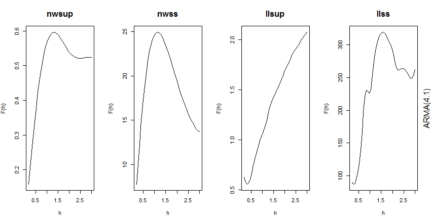
(a) F(h) using ARMA DGP under model (4.1)

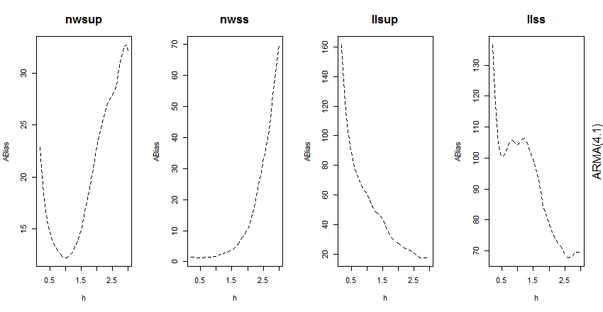
(b) ABias using ARMA DGP under model (4.1)

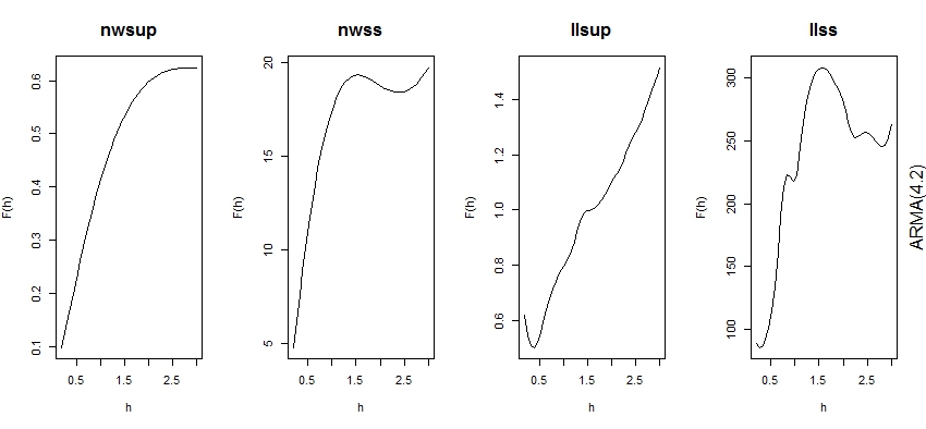
(c) F(h) using ARMA DGP under model (4.2)

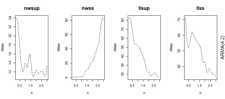
(d) ABias using ARMA DGP under model (4.2)

Fig. 1:  Simulating $X_{t}$ by ARMA(1,1) process and $\epsilon_{t}$ by N(0,0.25), we obtain the F(h) and ABias of each method. Note that each column corresponds to a detection method, and the first two rows demonstrate the experimental F(h) and ABias under the model (4.1) while the last two rows show those under the model (4.2) with $\Delta_{\varphi}=0.5$ without loss of generality.

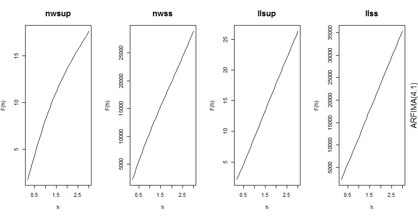
(a) F(h) using ARFIMA DGP under model (4.1)

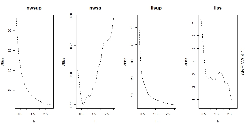
(b) ABias using ARFIMA DGP under model (4.1)

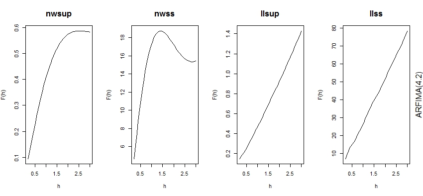
(c) F(h) using ARFIMA DGP under model (4.2)

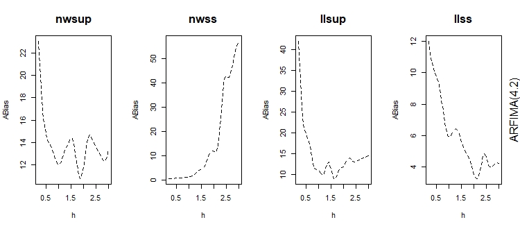
(d) ABias using ARFIMA DGP under model (4.2)

Fig. 2:  Simulating $X_{t}$ by ARFIMA(0,0.15,0) process and $\epsilon_{t}$ by ARFIMA(0,0.35,0) process, we obtain the F(h) and ABias of each method. Note that each column corresponds to a detection method, and the first two rows demonstrate the experimental F(h) and ABias under the model (4.1) while the last two rows show those under the model (4.2) with $\Delta_{\varphi}=0.5$ without loss of generality.

Now, we use bootstrap to determine the threshold $\xi_{n}$ of our method “nwss”. Specifically, we resample 200 sets of samples without replacing (which is a permutation essentially) and compute the 200 values of $\max_{t}W_{1,n}(t)$. Then we define the 99th percentile of $\max_{t}W_{1,n}(t)$’s as the threshold, which is an approximation of the order in Theorem 3.1. To show the performance of our detection and threshold determination, we replicate 500 detection experiments for each specification defined in Section 4.1. For each case, the percentage of experiments determining a change happens, denoted as PDC, is shown in Table 1, that is, the percentage of $\max_{t}W_{1,n}(t)>\xi_{n}$. PDC shows the rate of the true positive results when there is a change point or the rate of the false positive results when the system is stable and it can measure the detection performance well.

From the table, we can see that: (i) When the structural change is large, e.g., the model (4.1) and the model (4.2) with $\Delta_{\varphi}=0.3$ or 0.5, our method can detect nearly all the changes. (ii) When there is no change point, the rate of the false positive results is approximately 2% for strongly mixing process. (iii) The accuracy increases with the sample size. (iv) When the change point is not around the center ($\theta=0.2$), the rate of the true positive results is slightly inferior than that when $\theta=0.4$ but remains good as long as the sample size is relatively large. Note that the results are the same for $\theta=0.4$ and $\theta=0.2$ when $\Delta_{\varphi}=0$.

These results are in compliance with the theoretical results. The larger the sample size is, the more accuracy our method is. It is possible to repeat the resample in the bootstrap procedures more times and select a larger threshold, for example 99.9th percentile. When sample size is large enough, we are able to find a proper threshold. According to Theorem 3.1 and 3.2, $\max_{t}W_{1,n}(t)$ should be less than the threshold if there is no change and exceed the threshold when the change point exists.

We conclude that, although our research detection is performed by threshold method rather than hypothesis testing, our method still has a nice rate of the true positive and a low rate of the false positive to distinguish whether there is a change point.

$X_{t}$	model	PDC($\theta=0.4$)			PDC($\theta=0.2$)
		$n=200$	$n=500$	$n=1000$	$n=200$	$n=500$	$n=1000$
ARMA	4.1	0.982	1	1	0.940	1	1
	$4.2(\Delta_{\varphi}=0.5)$	0.888	0.998	1	0.722	0.956	1
	$4.2(\Delta_{\varphi}=0.3)$	0.678	0.924	1	0.562	0.748	0.942
	$4.2(\Delta_{\varphi}=0.1)$	0.036	0.264	0.108	0.014	0.234	0.064
	$4.2(\Delta_{\varphi}=0)$	0.018	0.012	0.016	0.018	0.012	0.016
ARFIMA	4.1	1	1	1	0.992	1	1
	$4.2(\Delta_{\varphi}=0.5)$	0.822	1	1	0.426	1	1
	$4.2(\Delta_{\varphi}=0.3)$	0.132	0.986	1	0.090	0.700	0.998
	$4.2(\Delta_{\varphi}=0.1)$	0.056	0.102	0.082	0.046	0.060	0.052
	$4.2(\Delta_{\varphi}=0)$	0.042	0.030	0.024	0.042	0.030	0.024

Table 1:  PDC under different models and data.

4.2 ARMA and ARFIMA processes with a change point

After judging whether there is a change point, to compare the estimation precision of the four methods,“nwss”, “nwsup”, “llss” and “llsup”, we do additional simulations under different model settings as below.

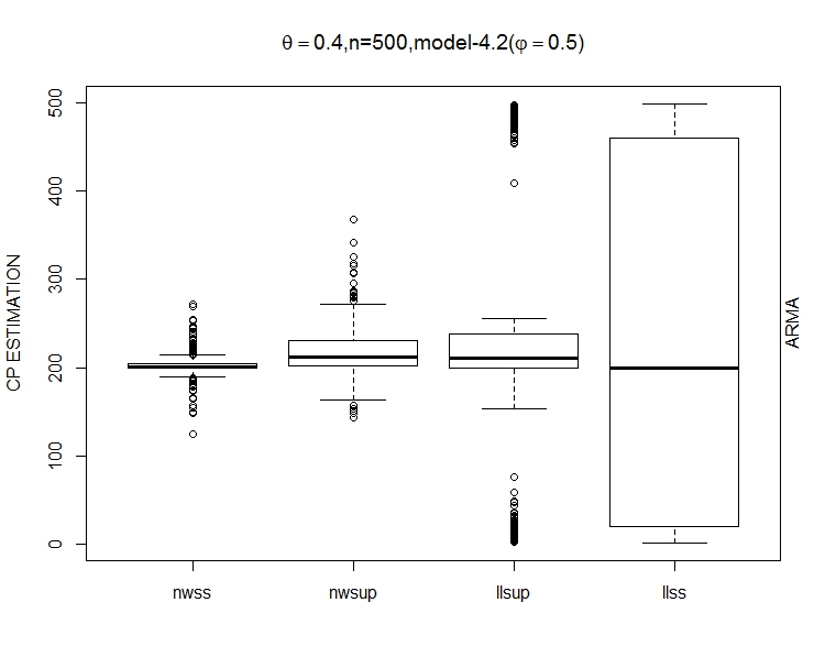
(b) $\theta=0.4,n=500$, and ARMA DGP under model (4.2)

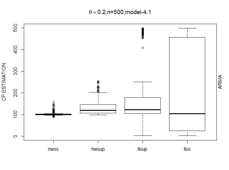
(c) $\theta=0.2,n=500$, and ARMA DGP under model (4.1)

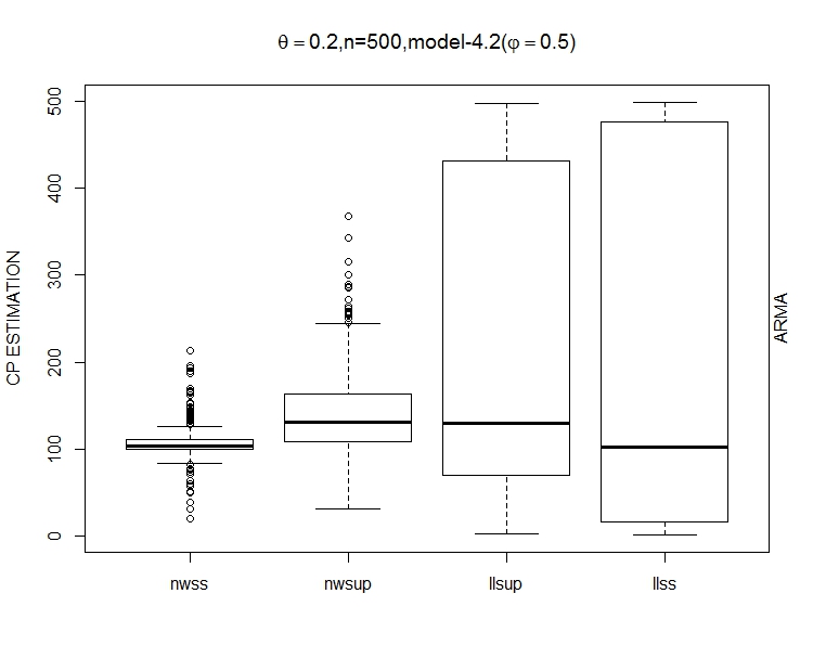
(d) $\theta=0.2,n=500$, and ARMA DGP under model (4.2)

Fig. 3:  At the case when data is generated by ARMA DGP, setting sample size $n=500$, we plot the box-plots of the change point estimates under the model (4.1) and the model (4.2) with $\theta=0.4$ and $\theta=0.2$, respectively.

Firstly, we generate ARMA DGP with the change point at $\theta=0.2$ and 0.4, and take the sample size $n=200,500$ and $1000$. We replicate 500 experiments for each case. The Bias and ABias of the estimators are shown in Table 2. For saving space and because of similarity, we select the case when $n=500$ with the model (4.1) and the model (4.2) ($\Delta_{\varphi}=0.5$), respectively, and plot the box-plots of the change point estimates in Figure 3. Note that the estimates outside $1.5\cdot{\sf IQR}$ from the median are marked by the void circle as outliers, where ${\sf IQR}$ means the interquartile range.

We can see from the table that “nwss” performs best among all cases and “nwss” estimator has far smaller “Bias” and “ABias” than other three methods. When the change point is near time boundary ($\theta=0.2$), the performance is still not bad as long as the structural change or sample size is not too small, despite it is inferior to that when the change point is about the central position. Intuitively, the local linear estimation may be superior to the N-W estimation. However, the result is opposite when they are introduced in the change-point detection procedure. Large “Bias”, “BiasSd”,“ABias” and “ABiasSd” are witnessed in most cases. We may call this phenomenon as the local linear paradox.

It is well known that the local linear fit is less influenced by outliers than the N-W fit, that is, the N-W estimation is more sensitive to outliers than the local linear estimation. Thus, we suspect that, when we use the local linear estimation, $|\widehat{\varphi}_{1,t}-\widehat{\varphi}_{t+1,n}|$ is flat around $t=k$ and $W_{1,n}(t)$ probably reaches the maximum at other time point when some stochastic errors exist. Thus, we will get the wrong estimate of the change point. While using N-W estimation, $|\widehat{\varphi}_{1,t}-\widehat{\varphi}_{t+1,n}|$ decreases quickly at around $t=k$ because of its sensitivity property, and we can obtain the maximum at the change point $k$. The stability advantage of the local linear fit develops disadvantage in this change-point detection and the local linear regression cannot be applied well to our detection in practice.

n	Model	Method	$\theta=0.4$				$\theta=0.2$
			Bias	BiasSd	ABias	ABiasSd	Bias	BiasSd	ABias	ABiasSd
n=200	4.1	nwss	2.126	7.233	2.802	6.998	5.278	14.034	5.938	13.767
		nwsup	9.406	8.813	9.570	8.634	22.110	22.453	22.158	22.406
		llsup	14.020	58.129	43.864	40.595	42.094	66.791	55.826	55.800
		llss	12.686	68.348	51.760	46.343	42.170	76.537	60.950	62.590
	4.2	nwss	2.013	16.465	8.963	13.951	8.313	22.781	12.722	20.638
	($\Delta_{\varphi}=0.5$)	nwsup	9.646	17.357	14.086	13.988	28.978	28.889	30.434	27.347
		llsup	14.106	68.767	57.806	39.750	47.644	74.360	66.068	58.568
		llss	14.362	74.272	61.334	44.201	43.322	80.185	65.522	63.313
	4.2	nwss	2.0678	34.870	23.277	26.015	21.871	47.352	30.505	42.289
	($\Delta_{\varphi}=0.3$)	nwsup	11.788	27.759	21.620	21.011	41.736	39.748	43.928	37.307
		llsup	16.316	76.542	69.908	35.050	53.682	79.217	74.818	59.615
		llss	14.042	82.441	75.686	35.416	51.082	85.440	77.166	62.834
n=500	4.1	nwss	1.192	3.463	1.788	3.196	2.728	6.877	3.236	6.653
		nwsup	12.228	12.586	12.236	12.578	30.756	30.899	30.768	30.887
		llsup	24.812	109.096	60.748	93.921	73.770	141.537	95.658	127.737
		llss	16.688	158.394	104.268	120.308	77.944	183.979	126.028	154.986
	4.2	nwss	3.098	12.404	6.889	10.767	6.845	18.480	10.949	16.381
	($\Delta_{\varphi}=0.5$)	nwsup	17.996	26.223	21.656	23.286	43.352	46.817	45.264	44.968
		llsup	25.834	146.082	99.294	110.134	93.622	176.052	135.626	146.102
		llss	21.488	174.659	126.644	122.056	87.646	197.860	144.898	160.649
	4.2	nwss	4.359	46.524	24.038	40.055	14.403	69.204	32.088	62.967
	($\Delta_{\varphi}=0.3$)	nwsup	19.922	46.556	35.034	36.542	71.740	79.929	76.080	75.801
		llsup	36.958	180.757	146.014	112.601	115.930	198.597	172.182	152.320
		llss	27.194	204.130	173.426	110.786	108.079	217.664	182.138	160.752
n=1000	4.1	nwss	1.732	4.743	2.280	4.505	2.188	5.593	2.504	5.462
		nwsup	15.914	18.122	15.930	18.108	42.434	45.790	42.442	45.783
		llsup	31.280	159.419	67.836	147.593	94.096	221.589	121.688	207.691
		llss	41.962	282.981	160.130	236.959	132.434	342.388	202.526	306.112
	4.2	nwss	3.464	9.112	5.616	7.965	6.730	16.901	9.570	15.469
	($\Delta_{\varphi}=0.5$)	nwsup	25.676	35.052	28.544	32.754	61.428	72.720	62.800	71.536
		llsup	37.054	228.565	119.742	198.119	137.230	305.007	191.638	274.044
		llss	45.342	312.549	196.314	247.246	148.852	373.300	243.264	319.779
	4.2	nwss	4.404	33.797	16.152	30.005	6.615	38.622	22.373	32.154
	($\Delta_{\varphi}=0.3$)	nwsup	32.278	59.658	46.874	49.005	96.584	113.546	100.448	110.136
		llsup	62.740	305.363	203.232	236.230	175.600	360.074	262.188	302.771
		llss	64.268	384.523	299.620	249.088	202.762	425.231	332.922	333.103

Table 2:  Simulating $X_{t}$ and $\epsilon_{t}$ by ARMA DGP, we replicate enormous experiments under different sample sizes, models and amounts of structural change. Then we compute the estimation bias of each method.

To compare our method “nwss” with “nwsup” in Wang (2008), we consider the long-memory DGP given by (4.4) and (4.5). The results are shown in Table 3 and Figure 4. Even for the long-memory data, “nwss” still has a superb performance with few big deviations as long as the structural change is not too tiny. While the method “nwsup” has relatively big bias and standard deviation. Also, the local linear paradox remains exist.

n	Model	Method	$\theta=0.4$				$\theta=0.2$
			Bias	BiasSd	ABias	ABiasSd	Bias	BiasSd	ABias	ABiasSd
n=200	4.1	nwss	0.786	1.870	0.858	1.838	1.745	4.203	1.806	4.177
		nwsup	6.698	7.370	6.702	7.367	16.330	19.211	16.334	19.207
		llsup	7.146	16.438	9.794	15.009	17.624	26.318	19.608	24.844
		llss	0.700	21.658	6.056	20.804	8.528	30.962	11.856	29.844
	4.2	nwss	1.673	10.756	4.861	9.737	6.807	22.572	9.718	21.475
	($\Delta_{\varphi}=0.5$)	nwsup	7.106	14.642	10.890	12.090	23.486	27.060	24.798	25.860
		llsup	7.448	26.129	13.888	23.346	21.586	36.812	25.422	34.270
		llss	1.394	28.162	9.482	26.551	7.820	34.338	12.140	33.056
	4.2	nwss	4.227	40.089	23.409	32.693	23.933	53.243	32.733	48.216
	($\Delta_{\varphi}=0.3$)	nwsup	9.984	25.850	18.652	20.482	33.624	36.117	35.928	33.821
		llsup	10.890	39.516	23.346	33.679	28.224	48.451	35.040	43.766
		llss	5.010	41.815	19.53	37.298	16.232	51.461	24.752	47.941
n=500	4.1	nwss	0.922	1.999	0.954	1.984	1.162	2.728	1.182	2.719
		nwsup	8.904	9.966	8.904	9.966	24.362	27.943	24.370	27.936
		llsup	11.076	24.188	13.168	23.114	28.236	39.803	29.464	38.901
		llss	0.696	37.550	6.708	36.952	11.318	59.164	15.502	58.206
	4.2	nwss	1.506	6.405	3.730	5.419	3.544	10.613	5.792	9.572
	($\Delta_{\varphi}=0.5$)	nwsup	13.208	21.384	15.984	19.393	38.590	44.179	39.530	43.338
		llsup	10.114	29.557	12.210	28.753	27.186	52.429	32.262	49.462
		llss	2.256	52.782	12.024	51.441	13.924	76.997	20.320	75.558
	4.2	nwss	2.184	25.692	11.762	22.939	5.550	41.453	16.631	38.258
	($\Delta_{\varphi}=0.3$)	nwsup	18.374	34.478	26.066	29.090	58.748	66.250	62.484	62.731
		llsup	8.156	53.917	21.940	49.914	39.048	83.426	49.576	77.620
		llss	6.146	78.835	25.726	74.764	25.374	107.586	38.206	103.717
n=1000	4.1	nwss	0.921	1.998	0.938	1.991	1.346	2.934	1.354	2.930
		nwsup	11.548	13.829	11.548	13.829	33.014	38.612	33.014	38.612
		llsup	15.088	28.843	15.088	28.843	39.944	53.390	40.628	52.871
		llss	1.368	56.758	7.500	56.276	15.296	101.836	20.520	100.912
	4.2	nwss	1.198	5.542	3.138	4.721	2.898	9.249	5.006	8.298
	($\Delta_{\varphi}=0.5$)	nwsup	14.156	23.915	16.780	22.149	54.828	64.433	55.952	63.457
		llsup	9.540	36.459	12.492	35.554	39.848	64.470	41.912	63.145
		llss	2.424	79.112	13.268	78.027	13.556	114.871	22.468	113.462
	4.2	nwss	2.610	29.752	8.870	28.516	5.829	45.781	13.036	44.268
	($\Delta_{\varphi}=0.3$)	nwsup	17.814	44.65646	29.966	37.582	75.358	90.264	77.698	88.253
		llsup	10.604	60.211	18.692	58.206	51.374	102.357	57.290	99.161
		llss	9.254	127.826	32.570	123.945	34.000	177.884	49.164	174.296

Table 3:  Simulating $X_{t}$ and $\epsilon_{t}$ by ARFIMA DGP, we replicate enormous experiments under different sample sizes, models and amounts of structural change. Then we compute the estimation bias of each method.

In conclusion, on one hand, our method is superior to other methods in each case and it performs well as long as the structural change is not too tiny and the change point is not too close to the edge, and the robust application to the long-memory data has been shown by ARFIMA DGP. On the other hand, “nwsup” tends to have a relatively bad performance. Last but not least, “llss” does not promote the effect and even results in big deviations in most cases, which pushes us only to use the simpler N-W estimation.

(a) $\theta=0.4,n=500$, and ARMA DGP under model (4.1)

(a) $\theta=0.4,n=500$, and ARFIMA DGP under model (4.1)

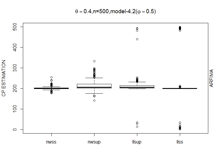
(b) $\theta=0.4,n=500$, and ARFIMA DGP under model (4.2)

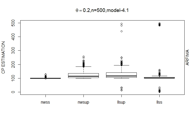
(c) $\theta=0.2,n=500$, and ARFIMA DGP under model (4.1)

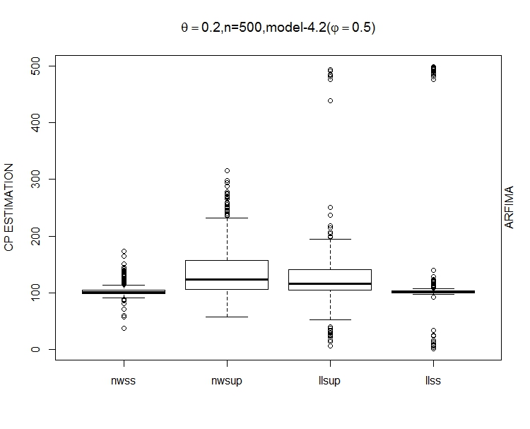
(d) $\theta=0.2,n=500$, and ARFIMA DGP under model (4.2)

Fig. 4:  At the case when data is generated by ARFIMA DGP, setting sample size $n=500$, we plot the box-plots of the change point estimates under the model (4.1) and the model (4.2) with $\theta=0.4$ and $\theta=0.2$, respectively.

5 Real data analysis

We apply our method to the Nasdaq 100 index for finding the structural change between the return volatility and the return. The relation between volatility and return is sometimes referred to as leverage effect, which can be illustrated as an asymmetric U-shaped curve. This relation can be time-varying, see for example Bandi and Renò (2012) and Jin (2017).

The volatility is inherently unobservable and we consider the realized volatility as the proxy of the return volatility. A discussion in gauging return-volatility regressions using different volatility measures can be found in Bollerslev and Zhou (2006). We take the three-year Nasdaq 100 index data from 2007–2009 as the sample (reader can acquire the data from the site https://realized.oxford-man.ox.ac.uk/data), and set its realized volatility as $Y_{t}$ and return as $X_{t}$. We plot the sequence $Y_{t}$ and $X_{t}$ in Figure 6, and think that there probably exists multiple change points. The dotted vertical lines mark the change-point positions computed later.

In order to select the bandwidth, we plot the curve $F(h)$ on the interval $(0,\max(X_{t})-\min(X_{t}))$ in Figure 5. It can be seen that $F(h)$ increases monotonically, so we choose the bandwidth $h=0.12$. Then we obtain the threshold by the permutation method as proposed in the simulation.

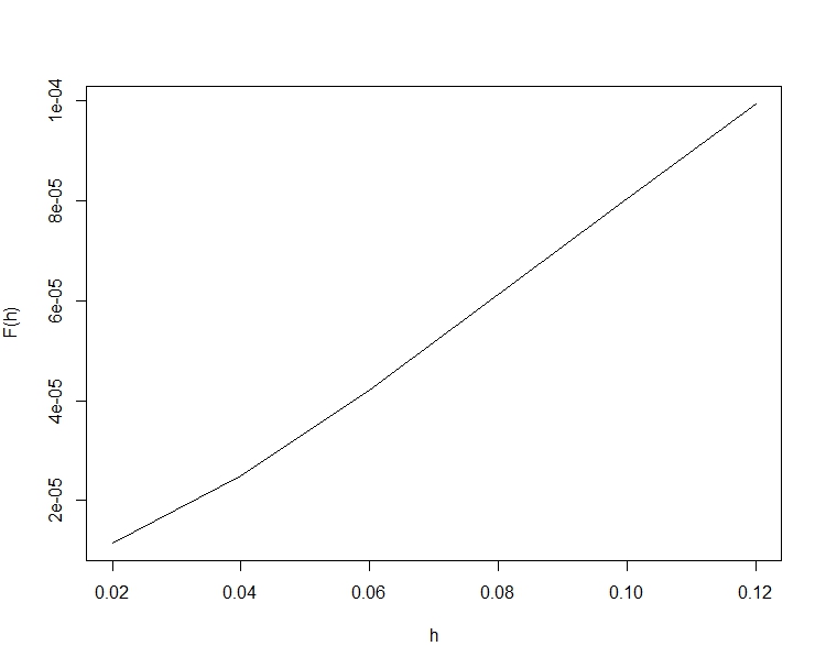
Fig. 5:  $F(h)$ based on Nasdaq index from 2007 to 2009

We detect the change point from the whole sample, and obtain the change point at 12/31/2007. Then we split the original sample to two sub-samples. Repeating the same steps for the left and right sub-samples, we detect the second change point 07/23/2007 and third one 06/02/2009. Note that the threshold is always changing because of the change of the sample size. Repeating the binary segmentation until the maximum of $W_{1,n}(t)$ of each sub-sample is less than the threshold or the sub-sample sizes are too few, we totally detect 16 change points (dates). We investigate the corresponding big financial events resulting in stock market to fluctuate just near the date in Table 4. We can expect that during the financial crisis, prices and volatility will be unstable. From our analysis, we can see that the relationship between price and volatility is also fragile, and change points occur very frequently.

To see how the leverage curve changes visually, we choose the first three detected change points 07/23/2007, 12/31/2007 and 06/02/2009 as the split points, and plot the four corresponding classical N-W kernel regression curves in Figure 7 with the bandwidth $h=0.01$. It is clear to find the obvious differences between $\widehat{\varphi}_{1}$ and $\widehat{\varphi}_{2}$, $\widehat{\varphi}_{2}$ and $\widehat{\varphi}_{3}$, $\widehat{\varphi}_{3}$ and $\widehat{\varphi}_{4}$, respectively.

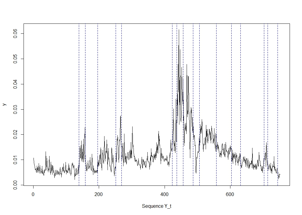
(a) The sequence of volatility $Y_{t}$

(b) The sequence of return $X_{t}$

Fig. 6:  The sequences of return $X_{t}$ and volatility $Y_{t}$

date (change point)	event	date (change point)	event
07/23/2007	Largest US commercial mortgage company	08/17/2007	American FED cut the window discount
	declared profit decreased by 33%		rate by 50 basis points to 5.75
10/10/2007	The dow Jones closed at	12/31/2007	International agricultural futures
	an all-time high of 14,165		prices continue to set new records
01/28/2008	American FED provided $30 billion	09/12/2008	The 4th large US investment
	to commercial bank		bank filed bankruptcy protection
10/02/2008	Bush signed a $700	10/29/2008	American sub-prime mortgage crisis
	billion financial rescue plan		developed to global financial crisis
12/12/2008	Many Banks in world cut	01/12/2009	The Finance of America injected
	interest rates in tandem once more		$14.77 billion into 43 Banks
03/26/2009	American FED declared to use $200 billion	06/02/2009	General motors officially filed for
	to help personal consumers and small enterprises		bankruptcy
07/13/2009	England bank announced it would	10/22/2009	The European debt crisis
	maintain QE at the 120 billion pounds		officially erupted
11/06/2009	England bank announced it would	12/21/2009	US House of Representatives passed the biggest
	increase QE 20 billion to 200 billion pounds		financial regulatory reform since 1930s

Table 4:  The probable change points and the big financial events around them

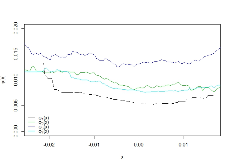
Fig. 7:  N-W kernel regression curves: $\varphi_{1}(x)$ from 01/03/2007 to 07/23/2007, $\varphi_{2}(x)$ from 07/23/2007 to 12/31/2007, $\varphi_{3}(x)$ from 12/31/2007 to 06/02/2009, $\varphi_{4}(x)$ from 06/02/2009 to 12/31/2009, respectively.

6 Conclusion and discussion

In this paper, firstly, we construct a CUSUM statistic to detect the structural change in the nonparametric regression model. The CUSUM statistic is constructed using sum-of-squares but not supremum like Wang (2008) so that we can find the relatively small structural change, especially when the function difference is small in the whole domain. Secondly, with probability one, we derive an upper bound of the CUSUM statistic asymptotically when there is no change point as well as a lower bound asymptotically when there is a change point. We establish the strong consistency of the change point estimator. Although we detect the change point by the threshold method not usual hypothesis testing, we still show in the simulation that our method has a low rate of the false positive and high rate of the true positive even if the structural change of the regression function is not obvious. Last but not least, we demonstrate a surprising result that the CUSUM method constructed by the N-W estimator performs better than that constructed by the local linear estimator, because the N-W estimator is more sensitive to the observations or outliers which do not belong to the same stable period.

Although we only focus on the case of one regressor and one change point, our method can be extended without difficulties to the multivariate regression with multiple change points.

Appendix: Proofs

In this section, we provide the detailed proofs of the theoretical results in Section 3. Before proving the main theorems, we state and prove some lemmas.

The following lemma plays a crucial role in deriving some uniform bounds of an $\alpha$-mixing process.

Lemma 1 (Theorem 1.3 of Bosq (1998))

Let $(X_{t},t\in\mathbb{Z})$ be a zero-mean real-valued process such that $\sup\limits_{1\leq t\leq n}\|X_{t}\|_{\infty}\leq b$. Let $S_{n}=\sum_{t=1}^{n}X_{t}$. Then
(i) For each integer $q\in[1,\frac{n}{2}]$ and each $\varepsilon>0$,

$${\sf P}(|S_{n}|>n\varepsilon)\leq 4\exp\left(-\frac{\varepsilon^{2}}{8b^{2}}q\right)+22\left(1+\frac{4b}{\varepsilon}\right)^{1/2}q\alpha\left(\left\lfloor\frac{n}{2q}\right\rfloor\right).$$

(ii) For each integer $q\in[1,\frac{n}{2}]$ and each $\varepsilon>0$,

$${\sf P}(|S_{n}|>n\varepsilon)\leq 4\exp\left(-\frac{\varepsilon^{2}}{8v^{2}(q)}q\right)+22\left(1+\frac{4b}{\varepsilon}\right)^{1/2}q\alpha\left(\left\lfloor\frac{n}{2q}\right\rfloor\right)$$

with $v^{2}(q)=\frac{2}{p^{2}}\sigma^{2}(q)+\frac{b\varepsilon}{2}$, $p=\frac{n}{2q}$,

$$\sigma^{2}(q) = \max_{0\leq j\leq 2q-1}{\sf E}\left\{(\lfloor jp\rfloor+1-jp)X_{\lfloor jp\rfloor+1}+X_{\lfloor jp\rfloor+2}+\right.$$

$$\left.\cdots+X_{\lfloor(j+1)p\rfloor}+((j+1)p-\lfloor(j+1)p\rfloor)X_{\lfloor(j+1)p+1\rfloor}\right\}^{2}.$$

The following lemma demonstrates the bounds of the auto-covariances of $K_{h_{n}}(x-X_{i})$ and $Y_{i}I_{(|Y_{i}|\leq T)}K_{h_{n}}(x-X_{i})$, that is, a truncated version of $Y_{i}K_{h_{n}}(x-X_{i})$, which facilitates the application of Lemma 1 to the N-W estimator.

Lemma 2

Suppose $\{X_{t},Y_{t}\}_{t=1}^{n}$ is an $\alpha$-mixing process, and Assumptions 4–6 are satisfied. Then we have
(i)

$${\sf Var}\left(K_{h_{n}}(x-X_{i})\right)\leq c_{1}h_{n}^{-1},$$ (6.1)

and

$$\left|{\sf Cov}\left(K_{h_{n}}(x-X_{i}),K_{h_{n}}(x-X_{j})\right)\right|\leq\left\{\begin{aligned} c_{2}\min\{h_{n}^{-1+q_{F}},h_{n}^{-2}|i-j|^{-\gamma}\},\{X_{t},Y_{t}\}_{t=1}^{n}\in PSM,\\ c_{2}\min\{h_{n}^{-1+q_{F}},h_{n}^{-2}\rho^{|i-j|}\}\ \ \ \ ,\{X_{t},Y_{t}\}_{t=1}^{n}\in GSM\\ \end{aligned}\right.$$ (6.2)

for any $1\leq i\neq j\leq n$ and $x\in\mathbb{R}$, where $c_{1}$ and $c_{2}$ are two positive constants, and $q_{F}$ is defined in Assumption 5.
(ii)

$${\sf Var}(Y_{i}I_{(|Y_{i}|\leq T)}K_{h_{n}}(x-X_{i}))\leq c_{3}h_{n}^{-1},$$ (6.3)

and

$$\left|{\sf Cov}\left(Y_{i}I_{(|Y_{i}|\leq T)}K_{h_{n}}(x-X_{i}),Y_{j}I_{(|Y_{j}|\leq T)}K_{h_{n}}(x-X_{j})\right)\right|$$ (6.4)

$$\leq \left\{\begin{aligned} c_{4}\min\{h_{n}^{-1+q_{F}},h_{n}^{-2}|i-j|^{-\gamma}\},\ \{X_{t},Y_{t}\}_{t=1}^{n}\in PSM,\\ c_{4}\min\{h_{n}^{-1+q_{F}},h_{n}^{-2}\rho^{|i-j|}\}\ \ \ \ \ ,\{X_{t},Y_{t}\}_{t=1}^{n}\in GSM\\ \end{aligned}\right.$$

for any $1\leq i\neq j\leq n$ and $x\in\mathbb{R}$, where $c_{3}$ and $c_{4}$ are two positive constants which does not dependent on $T$.

Proof of Lemma 2

(i) Noting that $f$, the density function of $X$, is uniformly bounded and $\|K\|_{2}<\infty$, we can prove that

$${\sf Var}(K_{h_{n}}(x-X_{i})) \leq {\sf E}\left[K_{h_{n}}^{2}(x-X_{i})\right]=\int_{\mathbb{R}}K_{h_{n}}^{2}(u-x)f(u)du$$

$$= h_{n}^{-1}\int_{\mathbb{R}}K^{2}(z)f(x+h_{n}z)dz\leq c_{1}h_{n}^{-1}$$

with variable substitution $z=(u-x)/h_{n}$ and selecting $c_{1}=\|f\|_{\infty}\|K\|_{2}^{2}$. In terms of the covariance, we have

$${\sf Cov}\left(K_{h_{n}}(x-X_{i}),K_{h_{n}}(x-X_{j})\right)$$

$$= {\sf E}\left[K_{h_{n}}(x-X_{i})K_{h_{n}}(x-X_{j})\right]-{\sf E}\left[K_{h_{n}}(x-X_{i})\right]{\sf E}\left[K_{h_{n}}(x-X_{j})\right]$$

$$= \int_{{\mathbb{R}}^{2}}K_{h_{n}}(x-u)K_{h_{n}}(x-v)F^{(|i-j|)}(u,v)dudv,$$

where $F^{(|i-j|)}$ is defined in Assumption 5. Letting $\bar{p_{F}}$ satisfy $p_{F}^{-1}+\bar{p_{F}}^{-1}=1$ and using Hölder inequality, we can prove that

$$\left|{\sf Cov}\left(K_{h_{n}}(x-X_{i}),K_{h_{n}}(x-X_{j})\right)\right|\leq h_{n}^{-2}\cdot h_{n}^{2/\bar{p_{F}}}\|K\|_{\bar{p_{F}}}^{2}\cdot\|F^{|i-j|}\|_{p_{F}}\leq c_{2,1}h_{n}^{-1+q_{F}},$$ (6.5)

where $c_{2,1}$ is equal to $\|K\|_{\bar{p_{F}}}^{2}\cdot C_{2}$, noting that $\|K\|_{\bar{p_{F}}}<\infty$, which is implied by $\|K\|_{1}<\infty$ and $\|K\|_{\infty}<\infty$ in Assumption 4. Besides, by using the Billingsley’s inequality (c.f. Chapter 1 of Bosq (1998)), we have

$$\left|{\sf Cov}\left(K_{h_{n}}(x-X_{i}),K_{h_{n}}(x-X_{j})\right)\right| \leq 4\|K_{h_{n}}(x-X_{i})\|_{\infty}\|K_{h_{n}}(x-X_{j})\|_{\infty}\cdot\alpha(|i-j|)$$ (6.6)

$$\leq c_{2,2}h_{n}^{-2}\alpha(|i-j|),$$

where $c_{2,2}=4\|K\|_{\infty}^{2}$. Note that we have $\alpha(|i-j|)\leq C_{1}\rho^{|i-j|}$ in Assumption 2 for GSM or $\alpha(|i-j|)\leq C_{1}|i-j|^{-\gamma}$ in Assumption 1 for PSM. Combining (6.5) and (6.6), and taking $c_{2}=\max\{c_{2,1},c_{2,2}C_{1}\}$, we can prove (6.2).

(ii) We denote $I_{(|Y_{i}|\leq T)}$ as $I_{i}$ for simplicity. Noting that $\|K\|_{2}<\infty$, $\|f\|_{\infty}<\infty$ and $\sup_{x\in{\sf supp}[X_{1}]}{\sf E}\left[Y_{i}^{2}|X_{i}=x\right]<C_{4}$ by Assumptions 4, 5 and 6, respectively, we have

$${\sf Var}(Y_{i}I_{i}K_{h_{n}}(x-X_{i}))\leq{\sf E}[Y_{i}^{2}K_{h_{n}}^{2}(x-X_{i})]=\int_{\mathbb{R}}{\sf E}[Y_{i}^{2}|X_{i}=u]K_{h_{n}}^{2}(x-u)f(u)du\leq c_{3}h_{n}^{-1}$$

by selecting $c_{3}=C_{4}\cdot\|f\|_{\infty}\cdot\|K\|_{2}^{2}$.

For the covariance, set $A=\{(y_{i},y_{j}):|y_{i}|\leq T,|y_{j}|\leq T\}$, we have

$$\left|{\sf Cov}\left(Y_{i}I_{i}K_{h_{n}}(x-X_{i}),Y_{j}I_{j}K_{h_{n}}(x-X_{j})\right)\right|$$

$$= \left|{\sf E}\left[Y_{i}I_{i}K_{h_{n}}(x-X_{i})\cdot Y_{j}I_{j}K_{h_{n}}(x-X_{j})\right]-{\sf E}\left[Y_{i}I_{i}K_{h_{n}}(x-X_{i})\right]\cdot{\sf E}[Y_{j}I_{j}K_{h_{n}}(x-X_{j})]\right|$$

$$= \left|\int_{\mathbb{R}^{2}}\int_{A}\left\{y_{i}y_{j}p(y_{i},y_{j},u,v)-y_{i}p(y_{i},u)\cdot y_{j}p(y_{j},v)\right\}dy_{i}dy_{j}\cdot K_{h_{n}}(x-u)K_{h_{n}}(x-v)dudv\right|$$

$$\leq \int_{\mathbb{R}^{2}}\int_{\mathbb{R}^{2}}\left|y_{i}y_{j}p(y_{i},y_{j},u,v)-y_{i}p(y_{i},u)y_{j}p(y_{j},v)\right|dy_{i}dy_{j}\cdot|K_{h_{n}}(x-u)K_{h_{n}}(x-v)|dudv$$

$$= \int_{\mathbb{R}^{2}}G^{|i-j|}(u,v)\cdot\left|K_{h_{n}}(x-u)K_{h_{n}}(x-v)\right|dudv$$

$$\leq h_{n}^{-2}\cdot h_{n}^{2/\bar{p_{G}}}\|K\|_{\bar{p_{G}}}^{2}\cdot\|G^{|i-j|}\|_{p_{G}}\leq c_{4,1}h_{n}^{-1+q_{G}},$$

where $c_{4,1}=C_{3}\|K\|_{\bar{p_{G}}}^{2}$ and $C_{3}$ are defined in Assumption 5. Note that the last step follows from the Hölder inequality similar to (6.5) with $\bar{p_{G}}$ satisfying $p_{G}^{-1}+\bar{p_{G}}^{-1}=1$.

Next we prove the second part in the minimization function in (6.4). Note that, for any $m\geq 1$ and $i=1,\cdots,n$,

$${\sf E}\left[|Y_{i}I_{i}K_{h_{n}}(X_{i}-x)|^{m}\right] \leq {\sf E}\left[|Y_{i}K_{h_{n}}(X_{i}-x)|^{m}\right]$$ (6.7)

$$\leq h_{n}^{-m}\cdot{\sf E}[|Y_{i}|^{m}]\cdot\|K\|_{\infty}^{m}=O(h_{n}^{-m}),$$

and $e^{C_{5}({\sf E}\left[|Y_{i}|^{m}\right])^{1/m}}\leq{\sf E}\left[e^{C_{5}|Y_{i}|}\right]\leq C_{6}$ by Assumption 6 and Jensen inequality. By Corollary 1.1 in Bosq (1998) together with (6.7), we have, for any $m>2$,

$$\left|{\sf Cov}\left(Y_{i}I_{i}K_{h_{n}}(X_{i}-x),Y_{j}I_{j}K_{h_{n}}(X_{j}-x)\right)\right|$$

$$\leq 2m/(m-2)\cdot(h_{n}^{-m}\cdot{\sf E}[|Y_{i}|^{m}]\cdot\|K\|_{\infty}^{m})^{2/m}\cdot[2\alpha([i-j])]^{1-2/m}$$

$$\leq c_{4,2}(m)\cdot h_{n}^{-2}\cdot[\alpha([i-j])]^{1-2/m}$$

with $c_{4,2}(m)=2^{2-2/m}\cdot m/(m-2)({\sf E}\left[|Y_{i}|^{m}\right]\|K\|_{\infty}^{m})^{2/m}$. Let $m$ tend to infinity, we have $c_{4,2}(m)\to 4\cdot(\log(C_{6})/C_{5})^{2}\|K\|_{\infty}^{2}:=c_{4,2}$, thus

$$\left|{\sf Cov}\left(Y_{i}I_{i}K_{h_{n}}(X_{i}-x),Y_{j}I_{j}K_{h_{n}}(X_{j}-x)\right)\right|\leq c_{4,2}\cdot h_{n}^{-2}\cdot\alpha([i-j]).$$

Using $\alpha(|i-j|)\leq C_{1}\rho^{|i-j|}$ in Assumption 2 or $\alpha(|i-j|)\leq C_{1}|i-j|^{-\gamma}$ in Assumption 1, and taking $c_{4}=\max\{c_{4,1},c_{4,2}C_{1}\}$, we can prove (6.4). $\Box$

The following lemma shows the uniform bound of the N-W estimator of a PSM process. Note that (i) the bandwidth is selected based on the sample size $n$, (ii) the estimator $\widehat{f}_{s,u}(x;h_{n})$ is constructed based on subsample set $\{X_{t},Y_{t}\}_{t=s}^{u}$, for $1\leq s\leq u\leq n$, and (iii) the uniform bound is considered with respect to time $t$.

Lemma 3

Suppose the process $\{X_{t},Y_{t}\}_{t=1}^{n}$ is PSM and Assumptions 3–6 are satisfied. Let $\widehat{f}_{1,t}(x;h_{n})$ and $\widehat{f}_{t+1,n}(x;h_{n})$ be defined in (2.4). Then we have for $\forall x\in\mathbb{R}$, under the model (2.1)

$$\max_{\Delta_{n}\leq t\leq n-\Delta_{n}}\left|\widehat{f}_{1,t}(x;h_{n})-{\sf E}\left[\widehat{f}_{1,t}(x;h_{n})\right]\right|=O_{a.s.}\left(\frac{\log n}{\sqrt{nh_{n}}}\right),$$ (6.8)

and

$$\max_{\Delta_{n}\leq t\leq n-\Delta_{n}}\left|\widehat{f}_{t+1,n}(x;h_{n})-{\sf E}\left[\widehat{f}_{t+1,n}(x;h_{n})\right]\right|=O_{a.s.}\left(\frac{\log n}{\sqrt{nh_{n}}}\right).$$ (6.9)

Proof of Lemma 3

It is clear that if for some $\eta>0$,

$$\sum_{n=1}^{\infty}{\sf P}\left(\max_{\Delta_{n}\leq t\leq n-\Delta_{n}}\left|\widehat{f}_{1,t}(x;h_{n})-{\sf E}\left[\widehat{f}_{1,t}(x;h_{n})\right]\right|>\eta\cdot\frac{\log n}{\sqrt{nh_{n}}}\right)<\infty,$$ (6.10)

we can show (6.8) by using the Borel-Cantelli lemma. Next we prove (6.10). Actually,

$${\sf P}\left(\max_{\Delta_{n}\leq t\leq n-\Delta_{n}}\left|\widehat{f}_{1,t}(x;h_{n})-{\sf E}\left[\widehat{f}_{1,t}(x;h_{n})\right]\right|>\eta\cdot\frac{\log n}{\sqrt{nh_{n}}}\right)$$

$$\leq \sum_{t=\Delta_{n}}^{n-\Delta_{n}}{\sf P}\left(\left|\widehat{f}_{1,t}(x;h_{n})-{\sf E}\left[\widehat{f}_{1,t}(x;h_{n})\right]\right|>\eta\cdot\frac{\log n}{\sqrt{nh_{n}}}\right)$$

$$\leq \sum_{t=\Delta_{n}}^{n-\Delta_{n}}{\sf P}\left(\left|\widehat{f}_{1,t}(x;h_{n})-{\sf E}\left[\widehat{f}_{1,t}(x;h_{n})\right]\right|>\eta\sqrt{\delta}\cdot\frac{\log t}{\sqrt{th_{n}}}\right),$$

noting that $\log n/\sqrt{n}>\sqrt{\delta}\log t/\sqrt{t}$ when $\lfloor n\delta\rfloor\leq t<n$. A sufficient condition is that for some $\eta>0$ and $\delta_{1}>0$

$${\sf P}\left(\left|\widehat{f}_{1,t}(x;h_{n})-{\sf E}\left[\widehat{f}_{1,t}(x;h_{n})\right]\right|>\eta\cdot\frac{\log t}{\sqrt{th_{n}}}\right)\leq c_{5}\cdot n^{-(2+\delta_{1})}$$ (6.11)

when $n$ is large enough, where $c_{5}$ is a positive constant (we still use the notation $\eta$ for $\eta\sqrt{\delta}$).

Next we prove (6.11) using Lemma 1(ii). Let $Z_{1,s,n}=K_{h_{n}}(x-X_{s})-{\sf E}\left[K_{h_{n}}(x-X_{s})\right]$ for $s=1,\cdots,n$, and denote the partial sum of $Z_{1,s,n}$ as $S_{t}=\sum_{s=1}^{t}Z_{1,s,n}$.

Firstly, we want to derive the order of $\sigma^{2}(q)$ and $v^{2}(q)$ defined in Lemma 1 with the sequence $\{X_{t}\}_{t=1}^{n}$ replaced by the sequence $\{Z_{1,s,n}\}_{s=1}^{t}$. Taking $\varepsilon=\varepsilon_{t}=(th_{n})^{-1/2}\log t$, $q=q_{t}=\lfloor t^{1/2}h_{n}^{-1/2}\rfloor$, and $p=t/(2q)$, we have $|Z_{1,s,n}|\leq\|K\|_{\infty}\cdot h_{n}^{-1}$ and $q_{t}\leq t/2$ for large n. Using the partition method similar to the proof of Theorem 3.3 in Johannes and Rao (2011), we have (define $p^{\prime}=\lfloor p\rfloor+2$)

$$\sigma^{2}(q) \leq \sum_{i=1}^{p^{\prime}}{\sf Var}(K_{h_{n}}(X_{i}-x))+2\sum_{i>j}^{p^{\prime}}|{\sf Cov}(K_{h_{n}}(X_{i}-x),K_{h_{n}}(X_{j}-x))|$$

$$= \sum_{i=1}^{p^{\prime}}{\sf Var}(K_{h_{n}}(X_{i}-x))+2\sum_{i=2}^{p^{\prime}}(p^{\prime}-i+1)|{\sf Cov}(K_{h_{n}}(X_{i}-x),K_{h_{n}}(X_{1}-x))|$$

$$\leq c_{1}p^{\prime}h_{n}^{-1}+2p^{\prime}\sum_{i=2}^{B}|{\sf Cov}(K_{h_{n}}(X_{i}-x),K_{h_{n}}(X_{1}-x))|$$

$$+ 2p^{\prime}\sum_{i=B+1}^{p^{\prime}}|{\sf Cov}(K_{h_{n}}(X_{i}-x),K_{h_{n}}(X_{1}-x))|$$

with the partition point $B=\lfloor h_{n}^{-q_{F}}\rfloor$. Then using Lemma 2, we can obtain for large n

$$\sigma^{2}(q) \leq c_{1}p^{\prime}h_{n}^{-1}+2p^{\prime}\sum_{i=2}^{B}c_{2}h_{n}^{-1+q_{F}}+2p^{\prime}\sum_{i=B+1}^{p^{\prime}}c_{2}h_{n}^{-2}(i-1)^{-\gamma}$$ (6.12)

$$\leq c_{1}p^{\prime}h_{n}^{-1}+2p^{\prime}B\cdot c_{2}h_{n}^{-1+q_{F}}+2p^{\prime}h_{n}^{-2}\cdot 2c_{2}B^{1-\gamma}$$

$$\leq c_{1}p^{\prime}h_{n}^{-1}+2p^{\prime}c_{2}h_{n}^{-q_{F}}\cdot h_{n}^{-1+q_{F}}+4c_{2}p^{\prime}h_{n}^{-2+q_{F}(\gamma-1)}$$

$$\leq (c_{1}+6c_{2})\cdot p^{\prime}h_{n}^{-1},$$

where the term $B^{1-\gamma}$ is induced by substituting the sum with an integral and the last row follows from $q_{F}(\gamma-1)>1$ in Assumption 5. So for $v^{2}(q)$, we have

$$v^{2}(q) = 2\sigma^{2}(q)/p^{2}+\|K\|_{\infty}\cdot h_{n}^{-1}\varepsilon_{t}/2$$ (6.13)

$$\leq 2(c_{1}+6c_{2})h_{n}^{-1}p^{\prime}p^{-2}+\|K\|_{\infty}\cdot h_{n}^{-1}\varepsilon_{t}/2$$

$$\leq \|K\|_{\infty}\cdot h_{n}^{-1}\varepsilon_{t}$$

for $n$ large enough, noting that $p^{\prime}/(p^{2})\simeq 2\varepsilon_{t}/\log t=o(\varepsilon_{t})$ when $\lfloor\delta n\rfloor\leq t\leq n-\lfloor\delta n\rfloor$. Then using Lemma 1(ii) and (6.13), we have for $\eta>0$

$$(6.13) = {\sf P}\left(\left|S_{t}\right|>t\cdot\eta\varepsilon_{t}\right)$$ (6.14)

$$\leq 4\exp\left(-\frac{\eta^{2}\varepsilon_{t}}{8\|K\|_{\infty}}q_{t}h_{n}\right)+22\left(1+\frac{4\|K\|_{\infty}\cdot h_{n}^{-1}}{\eta\varepsilon_{t}}\right)^{1/2}q\alpha\left(\left\lfloor\frac{t}{2q_{t}}\right\rfloor\right)$$

$$:= A_{1,t}+A_{2,t}.$$

Because $q_{t}\simeq t^{1/2}h_{n}^{-1/2}$ and thereby $\varepsilon_{t}q_{t}h_{n}\simeq(\log t)$, by selecting $\eta>\sqrt{8(2+\delta_{1})\|K\|_{\infty}}$, we have $A_{1,t}\leq 4t^{-{\eta^{2}}/(8\|K\|_{\infty})}=O\left(n^{-(2+\delta_{1})}\right)$. In terms of $A_{2,t}$, noting that $(h_{n}^{-1}/\varepsilon_{t})^{1/2}q_{t}\leq t^{3/4}h_{n}^{-3/4}\leq n^{3/4}h_{n}^{-3/4}\rightarrow\infty$ and $\alpha\left(\left\lfloor\frac{t}{2q_{t}}\right\rfloor\right)\leq C_{1}{\left\lfloor\frac{t}{2q_{t}}\right\rfloor}^{-\gamma}\leq C_{1}{\left\lfloor\frac{\sqrt{th_{n}}}{2}\right\rfloor}^{-\gamma}=O(n^{-\gamma/2}h_{n}^{-\gamma/2})$, we can obtain

$$A_{2,t}=O\left(n^{-\gamma/2+3/4}h_{n}^{-3/4-\gamma/2}\right)=O\left(n^{-(2+\delta_{1})}\right)$$

when $h_{n}\simeq n^{-\omega}$ for some $0<\omega\leq\frac{\gamma/2-11/4-\delta_{1}}{\gamma/2+3/4}<1-\frac{14}{2\gamma+3}$.

The proof of (6.9) is similar to the proof of (6.8) by considering the sequence $\{Z_{1,s,n}\}_{s=t+1}^{n}$. Thus we omit the proof. Then we complete the proof of this lemma. $\Box$

Lemma 4

Suppose the process $\{X_{t},Y_{t}\}_{t=1}^{n}$ is GSM and Assumptions 3–6 are satisfied. Let $\widehat{f}_{1,t}(x;h_{n})$ and $\widehat{f}_{t+1,n}(x;h_{n})$ be defined in (2.4), then we have for $\forall x\in\mathbb{R}$, under the model (2.1)

$$\max_{\ \Delta_{n}\leq t\leq n-\Delta_{n}}\left|\widehat{f}_{1,t}(x;h_{n})-{\sf E}\left[\widehat{f}_{1,t}(x;h_{n})\right]\right|=O_{a.s.}\left(\frac{\log n}{\sqrt{nh_{n}}}\right),$$ (6.15)

and

$$\max_{\ \Delta_{n}\leq t\leq n-\Delta_{n}}\left|\widehat{f}_{t+1,n}(x;h_{n})-{\sf E}\left[\widehat{f}_{t+1,n}(x;h_{n})\right]\right|=O_{a.s.}\left(\frac{\log n}{\sqrt{nh_{n}}}\right).$$ (6.16)

Proof of Lemma 4

The proof of this lemma is similar to the proof of Lemma 3. Because of similarity, we only prove (6.15).

We need to prove (6.11) by Lemma 1(ii). Using the same notation with Lemma 3, we have $\sigma^{2}(q)=O(p^{\prime}h_{n}^{-1})$, hence $v^{2}(q)\leq\|K\|_{\infty}\cdot h_{n}^{-1}\varepsilon_{t}$ for $n$ large enough (see Lemma 2.1 of Bosq (1998)). Then we still have (6.14). By selecting $\eta>\sqrt{8(2+\delta_{1})\|K\|_{\infty}}$, we have

$$A_{1,t}\leq 4t^{-{\eta^{2}}/(8\|K\|_{\infty})}=O\left(n^{-(2+\delta_{1})}\right).$$ (6.17)

In terms of $A_{2,t}$, note that $\log t/\sqrt{th_{n}}\rightarrow 0$, which implies that $th_{n}$ and thus $\log t-\log h_{n}^{-1}\rightarrow\infty$, and therefore $\log t$ and $\log h_{n}^{-1}$ can be bounded by $\sqrt{th_{n}}$. We have

$$A_{2,t} = 22\left(1+\frac{4\|K\|_{\infty}\cdot h_{n}^{-1}}{\eta\varepsilon_{t}}\right)^{1/2}q\alpha\left(\left\lfloor\frac{t}{2q_{t}}\right\rfloor\right)$$ (6.18)

$$\leq c_{7}\cdot t^{3/4}h_{n}^{-3/4}\cdot\rho^{\sqrt{th_{n}}/2}$$

$$= c_{7}\cdot\exp\left\{\frac{3}{4}\left(\log t+\log h_{n}^{-1}\right)\right\}\cdot\exp\left\{-\frac{1}{2}\log\left(\frac{1}{\rho}\right)\cdot\sqrt{th_{n}}\right\}$$

$$\leq c_{7}\cdot\exp\left\{-c_{8}\sqrt{th_{n}}\right\}$$

$$= c_{7}\cdot t^{-c_{8}/\varepsilon_{t}}=o\left(n^{-(2+\delta_{1})}\right),$$

where $c_{7}$ and $c_{8}$ are two positive constants, noting that $\varepsilon_{t}\rightarrow 0$. Combining (6.14), (6.17) and (6.18), we can prove (6.11). Thus we complete the proof of this lemma. $\Box$

Lemma 5

Suppose the process $\{X_{t},Y_{t}\}_{t=1}^{n}$ is PSM and Assumptions 3–6 are satisfied. Let $\widehat{g}_{1,t}(x;h_{n})$ and $\widehat{g}_{t+1,n}(x;h_{n})$ be defined in (2.3). Then we have for $\forall x\in\mathbb{R}$, under the model (2.1)

$$\ \max_{\Delta_{n}\leq t\leq n-\Delta_{n}}\left|\widehat{g}_{1,t}(x;h_{n})-{\sf E}[\widehat{g}_{1,t}(x;h_{n})]\right|=O_{a.s.}\left(\frac{\log^{2}n}{\sqrt{nh_{n}}}\right),$$ (6.19)

and

$$\ \max_{\Delta_{n}\leq t\leq n-\Delta_{n}}\left|\widehat{g}_{t+1,n}(x;h_{n})-{\sf E}[\widehat{g}_{t+1,n}(x;h_{n})]\right|=O_{a.s.}\left(\frac{\log^{2}n}{\sqrt{nh_{n}}}\right),$$ (6.20)

Proof of Lemma 5

The proof of this lemma is similar to that of Lemma 3. The only difference is that $Y_{i}$ may not be bounded, and we need to adopt the idea of truncation before using Lemma 1(ii). Analogously, our goal is to prove for some $\eta>0$

$$\sum_{n=1}^{\infty}{\sf P}\left(\max_{\Delta_{n}\leq t\leq n-\Delta_{n}}\left|\widehat{g}_{1,t}(x;h_{n})-{\sf E}\left[\widehat{g}_{1,t}(x;h_{n})\right]\right|>\eta\frac{\log^{2}n}{\sqrt{nh_{n}}}\right)<\infty,$$

which can be proved by

$${\sf P}\left(\left|\widehat{g}_{1,t}(x;h_{n})-{\sf E}[\widehat{g}_{1,t}(x;h_{n})]\right|>\eta\varepsilon_{t}\right)=O\left(n^{-(2+\delta_{1})}\right),$$ (6.21)

where $\varepsilon_{t}=\log^{2}t/\sqrt{th_{n}}$ and $\delta_{1}$ is a tiny positive constant.

Next, we prove (6.21). For $s=1,\cdots,n$ , define $\bar{Y}_{s}=Y_{s}I_{(|Y_{s}|\leq T_{t})}$ and $\widetilde{Y}_{s}=Y_{s}I_{(|Y_{s}|>T_{t})}$ with $T_{t}=c_{9}\log t$, where $c_{9}$ is a positive constant which will be determined later. Then

$$Z_{2,s,n} =: Y_{s}K_{h_{n}}(X_{s}-x)-{\sf E}[Y_{s}K_{h_{n}}(X_{s}-x)]$$ (6.22)

$$= (\bar{Y}_{s}K_{h_{n}}(X_{s}-x)-{\sf E}[\bar{Y}_{s}K_{h_{n}}(X_{s}-x)])$$

$$+(\widetilde{Y}_{s}K_{h_{n}}(X_{s}-x)-{\sf E}[\widetilde{Y}_{s}K_{h_{n}}(X_{s}-x)])$$

$$:= \bar{Z}_{2,s,n}+\widetilde{Z}_{2,s,n}.$$

Denote the partial sums in (6.22) as $\bar{S}_{t,n}=\sum_{s=1}^{t}\bar{Z}_{2,s,n}$ and $\widetilde{S}_{t,n}=\sum_{s=1}^{t}\widetilde{Z}_{2,s,n}$. To use Lemma 1(ii), set $q=q_{t}=\lfloor t^{1/2}h_{n}^{-1/2}\rfloor$. Then (6.21) can be written as follows,

$${\sf P}\left(\left|\widehat{g}_{1,t}(x;h_{n})-{\sf E}[\widehat{g}_{1,t}(x;h_{n})]\right|>\eta\varepsilon_{t}\right) = {\sf P}\left(|\bar{S}_{t,n}+\widetilde{S}_{t,n}|>t\cdot\eta\varepsilon_{t}\right)$$

$$\leq {\sf P}\left(|\bar{S}_{t,n}|>t\cdot\frac{\eta}{2}\varepsilon_{t}\right)+{\sf P}\left(|\widetilde{S}_{t,n}|>t\cdot\frac{\eta}{2}\varepsilon_{t}\right),$$

so we can prove this lemma by showing that

$${\sf P}\left(|\bar{S}_{t,n}|>t\cdot\frac{\eta}{2}\varepsilon_{t}\right)=O\left(n^{-(2+\delta_{1})}\right)$$ (6.23)

and

$${\sf P}\left(|\widetilde{S}_{t,n}|>t\cdot\frac{\eta}{2}\varepsilon_{t}\right)=O\left(n^{-(2+\delta_{1})}\right).$$ (6.24)

For (6.23), before using the similar method by the inequality in Lemma 1(ii) like before, we still need to show the bound of $\sigma^{2}(q)$. Together with Lemma 2(ii), it immediately follows that, like (6.12) by using $B=\lfloor h_{n}^{-q_{G}}\rfloor$, for large n

$$\sigma^{2}(q) \leq c_{3}p^{\prime}h_{n}^{-1}+2p^{\prime}\sum_{i=2}^{B}c_{4}h_{n}^{-1+q_{G}}+2p^{\prime}\sum_{i=B+1}^{p^{\prime}}c_{4}h_{n}^{-2}(i-1)^{-\gamma}$$

$$\leq c_{3}p^{\prime}h_{n}^{-1}+2p^{\prime}B\cdot c_{4}h_{n}^{-1+q_{G}}+2p^{\prime}h_{n}^{-2}c_{4}\cdot 2B^{1-\gamma}$$

$$\leq c_{3}p^{\prime}h_{n}^{-1}+2p^{\prime}c_{4}h_{n}^{-q_{G}}\cdot h_{n}^{-1+q_{G}}+4p^{\prime}c_{4}h_{n}^{-2+q_{G}(\gamma-1)}$$

$$\leq (c_{3}+6c_{4})\cdot p^{\prime}h_{n}^{-1}$$

when $q_{G}(\gamma-1)>1$. Hence

$$v^{2}(q)\leq\left(\frac{4(c_{3}+6c_{4})}{c_{9}\|K\|_{\infty}\log^{3}t}+1\right)\|K\|_{\infty}h_{n}^{-1}\varepsilon_{t}T_{t}\leq 2\|K\|_{\infty}h_{n}^{-1}\varepsilon_{t}T_{t}$$

when n is sufficiently large. Then we can use Lemma 1(ii) like the proof before and derive that for $\eta>0$

$${\sf P}\left(|\bar{S}_{t,n}|>t\cdot\frac{\eta}{2}\varepsilon_{t}\right) \leq 4\exp\left(-\frac{\eta^{2}\varepsilon_{t}}{64\|K\|_{\infty}T_{t}}qh_{n}\right)+22\left(1+\frac{16\|K\|_{\infty}h_{n}^{-1}T_{t}}{\eta\varepsilon_{t}}\right)^{1/2}q\alpha\left(\left\lfloor\frac{t}{2q}\right\rfloor\right)$$

$$:= A_{3,t}+A_{4,t}.$$

For $A_{3,t}$, we have

$$A_{3,t} \simeq 4\exp\left(-\frac{\eta^{2}}{64c_{9}\|K\|_{\infty}}\cdot\log t\right)=4t^{-\eta^{2}/(64c_{9}\|K\|_{\infty})}=O\left(n^{-(2+\delta_{1})}\right)$$

by selecting $\eta>8\sqrt{c_{9}(2+\delta_{1})\|K\|_{\infty}}$. For $A_{4,t}$, we have

$$A_{4,t} = 22\left(1+\frac{16c_{2}\|K\|_{\infty}\sqrt{t}}{\eta\sqrt{h_{n}}\log t}\right)^{1/2}\frac{\sqrt{t}}{\sqrt{h_{n}}}\left(\frac{\sqrt{th_{n}}}{4}\right)^{-\gamma}$$

$$\leq c_{10}\frac{t^{3/4-\gamma/2}}{h_{n}^{3/4+\gamma/2}}\frac{1}{\log^{1/2}t}$$

$$\leq c_{11}\frac{1}{n^{\gamma/2-3/4}h_{n}^{3/4+\gamma/2}}$$

$$= O\left(n^{-(2+\delta_{1})}\right),$$

where the existence of $\delta_{1}$ in the last equality follows from Assumption 3. Then we have proved (6.23).

In terms of (6.24), using Cauchy-Schwarz and Markov inequality, we have

$${\sf P}\left(|\widetilde{S}_{t,n}|>t\cdot\frac{\eta}{2}\varepsilon_{t}\right) \leq \frac{2{\sf E}\left[|\widetilde{S}_{t,n}|\right]}{t\eta\varepsilon_{t}}$$

$$\leq \frac{2{\sf E}\left[|Y_{1}K_{h}(X_{1}-x)I_{(|Y_{1}|>T_{t})}|\right]}{\eta\varepsilon_{t}}$$

$$\leq \frac{2\left\{\mathsf{E}\left[\left|Y_{1}K_{h}(X_{1}-x)\right|^{2}\right]\right\}^{1/2}\left\{\mathsf{P}\left(C_{5}\left|Y_{1}\right|>C_{5}T_{t}\right)\right\}^{1/2}}{\eta\varepsilon_{t}}$$

$$= \frac{2\left\{\int{\sf E}[Y_{1}^{2}|X_{1}=u]K_{h_{n}}^{2}(u-x)f(u)du\right\}^{1/2}\left\{\mathsf{P}(e^{C_{5}|Y_{1}|}>e^{C_{5}T_{t}})\right\}^{1/2}}{\eta\varepsilon_{t}}$$

$$= O\left(\frac{\sqrt{th_{n}}}{\log^{2}t}\cdot h_{n}^{-1/2}\cdot t^{-\frac{c_{9}C_{5}}{2}}\right)$$

$$= O\left(n^{-(2+\delta_{1})}\right)$$

by letting $c_{9}>(5+2\delta_{1})/C_{5}$, noting that $\|K\|_{2}<\infty$, $f$ is uniformly bounded, $\sup\limits_{x\in{\sf supp}[{X_{1}}]}{\sf E}\left[Y_{1}^{2}|X_{1}=x\right]<\infty$, and ${\sf E}\left[e^{C_{5}|Y_{1}|}\right]<\infty$.

Combing (6.23) and (6.24), we obtain (6.21). Hence the proof is completed. $\Box$

Lemma 6

Suppose the process $(X_{t},Y_{t})$ is GSM and Assumptions 3–6 are satisfied. Let $\widehat{g}_{1,t}(x;h_{n})$ and $\widehat{g}_{t+1,n}(x;h_{n})$ be defined in (2.3). Then we have for $\forall x\in\mathbb{R}$, under the model (2.1)

$$\max_{\Delta_{n}\leq t\leq n-\Delta_{n}}|\widehat{g}_{1,t}(x;h_{n})-{\sf E}[\widehat{g}_{1,t}(x;h_{n})]|=O_{a.s.}\left(\frac{\log^{2}n}{\sqrt{nh_{n}}}\right),$$ (6.25)

and

$$\max_{\Delta_{n}\leq t\leq n-\Delta_{n}}|\widehat{g}_{t+1,n}(x;h_{n})-{\sf E}[\widehat{g}_{t+1,n}(x;h_{n})]|=O_{a.s.}\left(\frac{\log^{2}n}{\sqrt{nh_{n}}}\right).$$ (6.26)

Proof of Lemma 6

We still use the notation in Lemma 5, and want to show (6.23) and (6.24). Together with Lemma 2(ii), it still holds that

$$\sigma^{2}(q) \leq c_{3}p^{\prime}h_{n}^{-1}+2p^{\prime}\left(\sum_{i=2}^{B}c_{4}h_{n}^{-1+q_{G}}+\sum_{i=B+1}^{p^{\prime}}c_{4}h_{n}^{-2}\rho^{(i-1)}\right)$$

$$\leq (c_{3}+2c_{4})p^{\prime}h_{n}^{-1}+2c_{4}p^{\prime}h_{n}^{-2}\cdot(1-\rho)^{-1}\rho^{h_{n}^{-q_{G}}}$$

$$= O(p^{\prime}h_{n}^{-1}),$$

noting that $\frac{p^{\prime}h_{n}^{-2}}{p^{\prime}h_{n}^{-1}}\cdot\rho^{h_{n}^{-q_{G}}}=h_{n}^{-1}\rho^{h_{n}^{-q_{G}}}\simeq(h_{n}^{-q_{G}})^{\frac{1}{q_{G}}}\cdot\rho^{h_{n}^{-q_{G}}}\rightarrow 0$. So we only need to show the part $A_{4,t}$ containing mixing-coefficient as follows,

$$A_{4,t} = 22\left(1+\frac{16\|K\|_{\infty}h_{n}^{-1}T_{t}}{\eta\varepsilon_{t}}\right)^{1/2}q\alpha\left(\left\lfloor\frac{t}{2q}\right\rfloor\right)\simeq 22\left(1+\frac{16c_{9}\|K\|_{\infty}\sqrt{t}}{\eta\sqrt{h_{n}}\log t}\right)^{1/2}\frac{\sqrt{t}}{\sqrt{h_{n}}}\cdot\rho^{\sqrt{th_{n}}/2}$$ (6.27)

$$\leq c_{12}\frac{t^{3/4}}{h_{n}^{3/4}}\frac{1}{\log^{1/2}t}\cdot\rho^{\sqrt{th_{n}}/2}$$

$$\leq c_{13}\exp\{-c_{14}\log^{2}t(\varepsilon_{t})^{-1}\}$$

$$= O\left(n^{-(2+\delta_{1})}\right),$$

where $c_{12},c_{13}$ and $c_{14}$ are strictly positive constants, noting that the last second row is deduced like (6.18), and $\varepsilon_{t}\rightarrow 0$. $\Box$

Lemma 7

Suppose that the assumptions in Lemmas 3 and 5 (or Lemmas 4 and 6) are satisfied. Let $\widehat{\varphi}_{1,t}(x;h_{n})$ and $\widehat{\varphi}_{t+1,n}(x;h_{n})$ be defined in (2.2). If the grid point $x_{i}\in\mathcal{X}$, then we have under the model (2.1)

$$\max\limits_{\Delta_{n}\leq t\leq n-\Delta_{n}}\left|\widehat{\varphi}_{1,t}(x_{i};h_{n})-\frac{{\sf E}[\widehat{g}_{1,t}(x_{i};h_{n})]}{{\sf E}[\widehat{f}_{1,t}(x_{i};h_{n})]}\right|=O_{a.s.}\left(\frac{\log^{2}n}{\sqrt{nh_{n}}}\right),$$ (6.28)

and

$$\max\limits_{\Delta_{n}\leq t\leq n-\Delta_{n}}\left|\widehat{\varphi}_{t+1,n}(x_{i};h_{n})-\frac{{\sf E}[\widehat{g}_{t+1,n}(x_{i};h_{n})]}{{\sf E}[\widehat{f}_{t+1,n}(x_{i};h_{n})]}\right|=O_{a.s.}\left(\frac{\log^{2}n}{\sqrt{nh_{n}}}\right).$$ (6.29)

Proof of Lemma 7

Because of similarity, we only show the first equation. Consider the decomposition

$$\widehat{\varphi}_{1,t}(x_{i})-\frac{{\sf E}[\widehat{g}_{1,t}(x_{i};h_{n})]}{{\sf E}[\widehat{f}_{1,t}(x_{i};h_{n})]}$$

$$= \frac{\widehat{g}_{1,t}(x_{i};h_{n})-\widehat{f}_{1,t}(x_{i};h_{n})\frac{{\sf E}[\widehat{g}_{1,t}(x_{i};h_{n})]}{{\sf E}[\widehat{f}_{1,t}(x_{i};h_{n})]}}{{\sf E}[\widehat{f}_{1,t}(x_{i};h_{n})]}$$

$$-\frac{\widehat{f}_{1,t}(x_{i};h_{n})-{\sf E}[\widehat{f}_{1,t}(x_{i};h_{n})]}{\widehat{f}_{1,t}(x_{i};h_{n})}\cdot\frac{\widehat{g}_{1,t}(x_{i};h_{n})-\widehat{f}_{1,t}(x_{i};h_{n})\frac{{\sf E}[\widehat{g}_{1,t}(x_{i};h_{n})]}{{\sf E}[\widehat{f}_{1,t}(x_{i};h_{n})]}}{{\sf E}[\widehat{f}_{1,t}(x_{i};h_{n})]}.$$

By Lemma 3, $\widehat{f}_{1,t}(x_{i};h_{n})-{\sf E}[\widehat{f}_{1,t}(x_{i};h_{n})]=o_{a.s.}(1)$ uniformly over $t$. Since $x_{i}\in{\cal X}=({\sf supp}[X_{1}])^{\circ}$, the density function $f$ has a nonzero lower bound in a sufficient small neighbourhood of $x_{i}$. We have ${\sf E}[\widehat{f}_{1,t}(x_{i};h_{n})]={\sf E}\left[K_{h_{n}}({X_{1}-x_{i}})\right]=h_{n}^{-1}\int_{\mathbb{R}}K((u-x_{i})/h_{n})f(u)du=\int_{\mathbb{R}}K(z)f(zh_{n}+x_{i})dz\geq c_{15}$ for some positive constant $c_{15}$ if $h_{n}$ is small enough. Then, by Lemma 3 and 5, we have

$$\max\limits_{\Delta_{n}\leq t\leq n-\Delta_{n}}\left|\widehat{\varphi}_{1,t}(x_{i};h_{n})-\frac{{\sf E}[\widehat{g}_{1,t}(x_{i};h_{n})]}{{\sf E}[\widehat{f}_{1,t}(x_{i};h_{n})]}\right|$$

$$= \max\limits_{\Delta_{n}\leq t\leq n-\Delta_{n}}\left|\frac{\widehat{g}_{1,t}(x_{i};h_{n})-\widehat{f}_{1,t}(x_{i};h_{n})\frac{{\sf E}[\widehat{g}_{1,t}(x_{i};h_{n})]}{{\sf E}[\widehat{f}_{1,t}(x_{i};h_{n})]}}{{\sf E}[\widehat{f}_{1,t}(x_{i};h_{n})]}\right|\left(1+o_{a.s.}(1)\right)$$

$$\leq \max\limits_{\Delta_{n}\leq t\leq n-\Delta_{n}}\left|\frac{\widehat{g}_{1,t}(x_{i};h_{n})-{\sf E}[\widehat{g}_{1,t}(x_{i};h_{n})]}{{\sf E}[\widehat{f}_{1,t}(x_{i};h_{n})]}\right|\left(1+o_{a.s.}(1)\right)$$

$$+\max\limits_{\Delta_{n}\leq t\leq n-\Delta_{n}}\left|\frac{\left(\widehat{f}_{1,t}(x_{i};h_{n})-{\sf E}[\widehat{f}_{1,t}(x_{i};h_{n})]\right)\frac{{\sf E}[\widehat{g}_{1,t}(x_{i};h_{n})]}{{\sf E}[\widehat{f}_{1,t}(x_{i};h_{n})]}}{{\sf E}[\widehat{f}_{1,t}(x_{i};h_{n})]}\right|\left(1+o_{a.s.}(1)\right)$$

$$= O_{a.s.}\left(\frac{\log^{2}n}{\sqrt{nh_{n}}}\right),$$

noting that ${\sf E}\left[|\widehat{g}_{1,t}(x_{i};h_{n})|\right]\leq{\sf E}\left[|Y_{i}K_{h_{n}}(X_{1}-x_{i})|\right]=\int_{\mathbb{R}}{\sf E}\left[|Y_{1}|\mid X_{1}=h_{n}z+x_{i}\right]\cdot K(z)f(h_{n}z+x_{i})dz\leq C_{4}||K||_{1}||f||_{\infty}$.

Hence we complete the proof of this lemma. $\Box$

Proof of Theorem 3.1

Since there is no change point, we have ${\sf E}[\widehat{f}_{1,t}(x_{i};h_{n})]={\sf E}[\widehat{f}_{t+1,n}(x_{i};h_{n})]$ and ${\sf E}[\widehat{g}_{1,t}(x_{i};h_{n})]={\sf E}[\widehat{g}_{t+1,n}(x_{i};h_{n})]$, and therefore by Lemma 7

$$\max\limits_{\Delta_{n}\leq t\leq n-\Delta_{n}}W_{1,n}(t) \leq 2\max\limits_{\Delta_{n}\leq t\leq n-\Delta_{n}}\sum_{i=1}^{m}\left|\widehat{\varphi}_{1,t}(x_{i};h_{n})-\frac{{\sf E}[\widehat{g}_{1,t}(x_{i};h_{n})]}{{\sf E}[\widehat{f}_{1,t}(x_{i};h_{n})]}\right|^{2}$$

$$+ 2\max\limits_{\Delta_{n}\leq t\leq n-\Delta_{n}}\sum_{i=1}^{m}\left|\widehat{\varphi}_{t+1,n}(x_{i};h_{n})-\frac{{\sf E}[\widehat{g}_{t+1,n}(x_{i};h_{n})]}{{\sf E}[\widehat{f}_{t+1,n}(x_{i};h_{n})]}\right|^{2}$$

$$= O_{a.s.}\left(\frac{\log^{4}n}{nh_{n}}\right).$$

We complete the proof of the theorem. $\Box$

Proof of Theorem 3.2

By definition,

$$\Lambda_{h_{n}}^{2}(x_{i}) = \left({\sf E}\left[\left(\varphi_{1}(X_{1})-\varphi_{2}(X_{1})\right)K_{h_{n}}(x_{i}-X_{1})\right]\right)^{2}/({\sf E}[K_{h_{n}}(X_{1}-x_{i})])^{2}$$

$$= \left(\int_{\mathbb{R}}(\varphi_{1}(u)-\varphi_{2}(u))K_{h_{n}}(x_{i}-u)f(u)du\right)^{2}/({\sf E}[K_{h_{n}}(X_{1}-x_{i})])^{2}$$

$$= \left(\int_{u\in\mathcal{X}\cap\mathcal{Y}}\left(\varphi_{1}(u)-\varphi_{2}(u)\right)K_{h_{n}}(x_{i}-u)f(u)du\right)^{2}/({\sf E}[K_{h_{n}}(X_{1}-x_{i})])^{2}$$

$$= \left(\int_{(h_{n}z+x_{i})\in\mathcal{X}\cap\mathcal{Y}}\left(\varphi_{1}(h_{n}z+x_{i})-\varphi_{2}(h_{n}z+x_{i})\right)K(z)f(h_{n}z+x_{i})dz\right)^{2}/({\sf E}[K_{h_{n}}(X_{1}-x_{i})])^{2}.$$

Note that $({\sf E}[K_{h_{n}}(X_{1}-x_{i})])$ is bounded. When $x_{i}\in\mathcal{X}\cap\mathcal{Y}$, both $\varphi_{1}(x)-\varphi_{2}(x)$ and $f(x)$ are bounded away from zero in a small neighbour of $x_{i}$. Therefore $\Lambda_{h_{n}}^{2}(x_{i})$ is also bounded away from zero when $n$ is large enough.

Next we prove (3.2). Considering the special point $t=k$, it is obvious that

$$\max\limits_{\Delta_{n}\leq t<n-\Delta_{n}}W_{1,n}(t)\geq W_{1,n}(k).$$

Note that the sequences $\{X_{s},Y_{s}\}_{s=1}^{k}$ and $\{X_{s},Y_{s}\}_{s=k+1}^{n}$ are strictly stationary. By definition and Lemma 7, we have

$$W_{1,n}(k) = \frac{k(n-k)}{n^{2}}\sum_{i=1}^{m}\left|\widehat{\varphi}_{1,k}(x_{i};h_{n})-\widehat{\varphi}_{k+1,n}(x_{i};h_{n})\right|^{2}$$ (6.30)

$$= \theta(1-\theta)\sum_{i=1}^{m}\left(\frac{{\sf E}[\widehat{g}_{1,k}(x_{i};h_{n})]}{{\sf E}[\widehat{f}_{1,k}(x_{i};h_{n})]}-\frac{{\sf E}[\widehat{g}_{k+1,n}(x_{i};h_{n})]}{{\sf E}[\widehat{f}_{k+1,n}(x_{i};h_{n})]}\right)^{2}+O_{a.s.}\left(\frac{\log^{2}n}{\sqrt{nh_{n}}}\right)$$

$$= \theta(1-\theta)\sum_{i=1}^{m}\Lambda^{2}_{h_{n}}(x_{i})+O_{a.s.}\left(\frac{\log^{2}n}{\sqrt{nh_{n}}}\right).$$

Thus, we complete the proof of this theorem. $\Box$

Proof of Theorem 3.3

(i) It is a direct corollary from Theorem 3.1 and 3.2.

Now we prove (ii). From the statement in the proof of Theorem 3.2, we have

$$\max\limits_{\Delta_{n}\leq t\leq k}W_{1,n}(t)\geq\theta(1-\theta)\sum_{i=1}^{m}\Lambda^{2}_{h_{n}}(x_{i})$$ (6.31)

almost surely when $n\rightarrow\infty$. If we can show that

$$\max\limits_{\Delta_{n}\leq t\leq k-n\varepsilon}W_{1,n}(t)<\theta(1-\theta)\sum_{i=1}^{m}\Lambda^{2}_{h_{n}}(x_{i})$$ (6.32)

almost surely, for any small $\epsilon>0$ when $n\rightarrow\infty$, then (6.31) and (6.32) imply that $\widehat{k}\geq k-n\varepsilon$ almost surely when $n\rightarrow\infty$. Using the same method for the case when $k+n\varepsilon\leq t\leq n-\Delta_{n}$, we can obtain $\widehat{k}\leq k+n\varepsilon$ almost surely when $n\rightarrow\infty$. Combining these two inequalities we can show that $(\widehat{k}-k)/n=o_{a.s.}(1)$ by letting $\varepsilon\rightarrow 0$.

Next we prove (6.32). When $t\leq k-n\varepsilon$, on the one hand, we have

$$\widehat{\varphi}_{1,t}(x_{i};h_{n})-\frac{{\sf E}[\widehat{g}_{1,t}(x_{i};h_{n})]}{{\sf E}[\widehat{f}_{1,t}(x_{i};h_{n})]}=O_{a.s.}\left(\frac{\log^{2}n}{\sqrt{nh_{n}}}\right)$$ (6.33)

uniformly in $t$ by Lemma 7. On the other hand,

$$\widehat{\varphi}_{t+1,n}(x_{i};h_{n})-\frac{{\sf E}[\widehat{g}_{1,t}(x_{i};h_{n})]}{{\sf E}[\widehat{f}_{1,t}(x_{i};h_{n})]}=\frac{\widehat{g}_{t+1,n}(x_{i};h_{n})}{\widehat{f}_{t+1,n}(x_{i};h_{n})}-\frac{{\sf E}[\widehat{g}_{1,t}(x_{i};h_{n})]}{{\sf E}[\widehat{f}_{1,t}(x_{i};h_{n})]}$$

$$= \frac{(k-t)\left(\widehat{g}_{t+1,k}(x_{i};h_{n})-{\sf E}[\widehat{g}_{t+1,k}(x_{i};h_{n})]\right)+(n-k)\left(\widehat{g}_{k+1,n}(x_{i};h_{n})-{\sf E}[\widehat{g}_{k+1,n}(x_{i};h_{n})]\right)}{(n-t)\widehat{f}_{t+1,n}(x_{i};h_{n})}$$

$$+ \frac{(k-t){\sf E}[g_{t+1,k}(x_{i};h_{n})]+(n-k){\sf E}[g_{k+1,n}(x_{i};h_{n})]-(n-t)\widehat{f}_{t+1,n}(x_{i};h_{n})\frac{{\sf E}[\widehat{g}_{1,t}(x_{i};h_{n})]}{{\sf E}[\widehat{f}_{1,t}(x_{i};h_{n})]}}{(n-t)\widehat{f}_{t+1,n}(x_{i};h_{n})}$$

$$:= B_{3}(x_{i})+B_{4}(x_{i}).$$

We show that $B_{3}(x_{i})$ is negligible and $B_{4}(x_{i})$ is the leading term. Similar to the argument of proof for Lemma 5, we can show that the asymptotic order of $\widehat{g}_{t+1,k}(x_{i};h_{n})-{\sf E}[\widehat{g}_{t+1,k}(x_{i};h_{n})]$ is also $\frac{\log^{2}n}{\sqrt{nh_{n}}}$, as the sample size $k-t$ is of order $n$. Note that $\widehat{f}_{t+1,n}$ is bounded away from zero almost surely when $n$ is large enough. Since $(k-t)/(n-t)<\theta/(1-\theta)$ and $(n-k)/(n-t)<1$, we have by Lemma 5 (or Lemma 6)

$$B_{3}(x_{i})=O_{a.s.}\left(\frac{\log^{2}n}{\sqrt{nh_{n}}}\right).$$ (6.34)

In terms of $B_{4}(x_{i})$, we have by Lemma 3

$$(n-t)\widehat{f}_{t+1,n}(x_{i};h_{n})=(k-t){\sf E}[\widehat{f}_{1,k}(x_{i};h_{n})]+(n-k){\sf E}[\widehat{f}_{k+1,n}(x_{i};h_{n})]+O_{a.s.}\left(\frac{n\log n}{\sqrt{nh_{n}}}\right).$$

Therefore,

$$B_{4}(x_{i}) = \frac{(k-t){\sf E}[\widehat{g}_{1,k}(x_{i};h_{n})]+(n-k){\sf E}[\widehat{g}_{k+1,n}(x_{i};h_{n})]}{(k-t){\sf E}[\widehat{f}_{1,k}(x_{i};h_{n})]+(n-k){\sf E}[\widehat{f}_{k+1,n}(x_{i};h_{n})]}-\frac{{\sf E}[\widehat{g}_{1,t}(x_{i};h_{n})]}{{\sf E}[\widehat{f}_{1,t}(x_{i};h_{n})]}+O_{a.s.}\left(\frac{\log^{2}n}{\sqrt{nh_{n}}}\right)$$ (6.35)

$$= \frac{(k-t){\sf E}[\widehat{g}_{1,k}(x_{i};h_{n})]+(n-k){\sf E}[\widehat{g}_{k+1,n}(x_{i};h_{n})]}{(k-t){\sf E}[\widehat{f}_{1,k}(x_{i};h_{n})]+(n-k){\sf E}[\widehat{f}_{k+1,n}(x_{i};h_{n})]}$$

$$-\frac{\left((k-t){\sf E}[\widehat{f}_{1,k}(x_{i};h_{n})]+(n-k){\sf E}[\widehat{f}_{k+1,n}(x_{i};h_{n})]\right)\frac{{\sf E}[\widehat{g}_{1,t}(x_{i};h_{n})]}{{\sf E}[\widehat{f}_{1,t}(x_{i};h_{n})]}}{(k-t){\sf E}[\widehat{f}_{1,k}(x_{i};h_{n})]+(n-k){\sf E}[\widehat{f}_{k+1,n}(x_{i};h_{n})]}+O_{a.s.}\left(\frac{\log^{2}n}{\sqrt{nh_{n}}}\right)$$

$$= \frac{(n-k){\sf E}[\widehat{f}_{k+1,n}(x_{i};h_{n})]}{(k-t){\sf E}[\widehat{f}_{1,k}(x_{i};h_{n})]+(n-k){\sf E}[\widehat{f}_{k+1,n}(x_{i};h_{n})]}\cdot\left(\frac{{\sf E}[\widehat{g}_{k+1,n}(x_{i};h_{n})]}{{\sf E}[\widehat{f}_{k+1,n}(x_{i};h_{n})]}-\frac{{\sf E}[\widehat{g}_{1,t}(x_{i};h_{n})]}{{\sf E}[\widehat{f}_{1,t}(x_{i};h_{n})]}\right)$$

$$+O_{a.s.}\left(\frac{\log^{2}n}{\sqrt{nh_{n}}}\right).$$

Combining (6.33)–(6.35), we can obtain uniformly in $t$

$$W_{1,n}(t) = \frac{t(n-t)}{n^{2}}\sum\limits_{i=1}\limits^{m}|\widehat{\varphi}_{1,t}(x_{i};h_{n})-\widehat{\varphi}_{t+1,n}(x_{i};h_{n})|^{2}$$

$$= \frac{t(n-t)}{n^{2}}\sum\limits_{i=1}\limits^{m}B_{4}^{2}(x_{i})+O_{a.s.}\left(\frac{\log^{2}n}{\sqrt{nh_{n}}}\right)$$

$$= \frac{t(n-t)}{n^{2}}\cdot\frac{(n-k)^{2}}{(n-t)^{2}}\sum\limits_{i=1}\limits^{m}\Lambda^{2}_{h_{n}}(x_{i})+O_{a.s.}\left(\frac{\log^{2}n}{\sqrt{nh_{n}}}\right)$$

$$= \frac{t(n-k)^{2}}{n^{2}(n-t)}\sum\limits_{i=1}\limits^{m}\Lambda^{2}_{h_{n}}(x_{i})+O_{a.s.}\left(\frac{\log^{2}n}{\sqrt{nh_{n}}}\right).$$

Note that

$$\frac{t(n-k)^{2}}{n^{2}(n-t)}\leq(1-\theta)^{2}\frac{\theta-\varepsilon}{1-\theta+\varepsilon}=(1-\theta)\cdot\frac{1-\theta}{1-\theta+\varepsilon}\cdot(\theta-\varepsilon)<\theta(1-\theta).$$

Thus, we have (6.32), and we complete the proof. $\Box$

References

• Aue, Rice and Sönmez (2018) Aue A, Rice G and Sönmez O(2018)Detecting and dating structural breaks in functional data without dimension reduction. Journal of the Royal Statistical Society: Series B 80(3): 509–529
• Bai (1997) Bai J(1997)Estimating multiple breaks one at a time. Econometric theory 13(3): 315–352
• Bandi and Renò (2012) Bandi FM and Renò R (2012)Time-varying leverage effects. Journal of Econometrics 169(1): 94-113
• Barigozzi, Cho and Fryzlewicz (2018) Barigozzi M, Cho H and Fryzlewicz P(2018)Simultaneous multiple change-point and factor analysis for high-dimensional time series. Journal of Econometrics 206(1): 187-225
• Basrak, Davis and Mikosch (2002) Basrak B, Davis RA and Mikosch T(2002)Regular variation of GARCH processes. Stochastic Processes and their Applications 99(1): 95–115
• Bollerslev and Zhou (2006) Bollerslev T and Zhou H(2006)Volatility puzzles: a simple framework for gauging return-volatility regressions. Journal of Econometrics 131(1-2): 123-150
• Bosq (1998) Bosq D(1998)Nonparametric Statistics for Stochastic Processes: Estimation and Prediction, 2nd edn. Springer-Verlag, New York
• Braun and Müller (1998) Braun JV and Müller HG(1998)Statistical methods for DNA sequence segmentation. Statistical Science 13(2): 142–162
• Brown, Durbin and Evans (1975) Brown RL, Durbin J and Evans JM(1975)Techniques for testing the constancy of regression relationships over time. Journal of the Royal Statistical Society: Series B 37(2): 149–192
• Chen and Nkurunziza (2017) Chen F and Nkurunziza S(2017)On estimation of the change points in multivariate regression models with structural changes. Communications in Statistics-Theory and Methods 46(14): 7157–7173
• Cho (2016) Cho H(2016)Change-point detection in panel data via double CUSUM statistic. Electronic Journal of Statistics 10(2): 2000–2038
• Cho and Fryzlewicz (2012) Cho H and Fryzlewicz P(2012)Multiscale and multilevel technique for consistent segmentation of nonstationary time series. Statistica Sinica 22: 207–229
• Cho and Fryzlewicz (2015) Cho H and Fryzlewicz P(2015)Multiple-change-point detection for high dimensional time series via sparsified binary segmentation. Journal of the Royal Statistical Society: Series B 77(2): 475–507
• Choi and Lee (2017) Choi JY and Lee MJ(2017)Regression discontinuity: review with extensions. Statistical Papers 58(4): 1217–1246
• Dette, Kokot and Aue (2017) Dette H, Kokot K and Aue A(2017)Functional data analysis in the Banach space of continuous functions. Preprint on https://arxiv.org/abs/1710.07781
• Delgado and Hidalgo (2000) Delgado MA and Hidalgo J. (2000). Nonparametric inference on structural breaks. Journal of Econometrics 96(1): 113-144
• Eichinger and Kirch (2018) Eichinger B and Kirch C(2018)A MOSUM procedure for the estimation of multiple random change points. Bernoulli 24(1): 526–564
• Enikeeva and Harchaoui (2019) Enikeeva F and Harchaoui Z(2019)High-dimensional change-point detection under sparse alternatives. The Annals of Statistics 47(4): 2051–2079
• Fryzlewicz (2014) Fryzlewicz P(2014)Wild binary segmentation for multiple change-point detection. The Annals of Statistics 42(6): 2243–2281
• Gurevich and Vexler (2005) Gurevich G and Vexler A(2005)Change point problems in the model of logistic regression. Journal of Statistical Planning and Inference 131(2): 313-331
• Härdle, Müller, Sperlich and Werwatz (2004) Härdle W, Müller M, Sperlich S and Werwatz A(2004)Nonparametric and Semiparametric Models. Springer-Verlag, Berlin Heidelberg
• Hosking (1981) Hosking JRM(1981)Fractional differencing. Biometrika 68(1): 165–176
• Huh and Park (2004) Huh J and Park BU(2004)Detection of a change point with local polynomial fits for the random design case. Australian and New Zealand Journal of Statistics 46(3): 425–441
• Hušková and Maciak (2017) Hušková M and Maciak M(2017)Discontinuities in robust nonparametric regression with $\alpha$-mixing dependence. Journal of Nonparametric Statistics 29(2): 447–475
• Hušková and Steinebach (2002) Hušková M and Steinebach J(2002)Asymptotic tests for gradual changes. Statistics and Risk Modeling 20(1-4): 137–152
• Jin (2017) Jin X(2017)Time-varying return-volatility relation in international stock markets. International Review of Economics & Finance 51: 157-173.
• Johannes and Rao (2011) Johannes J and Rao SS(2011)Nonparametric estimation for dependent data. Journal of Nonparametric Statistics 23(3): 661–681
• Kaul, Jandhyala and Fotopoulos (2019) Kaul A, Jandhyala VK and Fotopoulos SB(2019)An efficient two step algorithm for high dimensional change point regression models without grid search. Journal of Machine Learning Research 20(111): 1–40
• Killick, Fearnhead and Eckley (2012) Killick R, Fearnhead P and Eckley IA(2012)Optimal detection of changepoints with a linear computational cost. Journal of the American Statistical Association 107(500): 1590–1598
• Masry (1996) Masry E(1996)Multivariate local polynomial regression for time series: uniform strong consistency and rates. Journal of Time Series Analysis 17(6): 571–599
• Mohr and Neumeyer (2019) Mohr M and Neumeyer N(2019)Consistent nonparametric change point detection combining CUSUM and marked empirical processes. Preprint on https://arxiv.org/abs/1901.08491
• Mohr and Selk (2020) Mohr M and Selk L(2020)Estimating change points in nonparametric time series regression models. Statistical Papers, online https://doi.org/10.1007/s00362-020-01162-8
• Müller (1992) Müller HG(1992)Change-points in nonparametric regression analysis. The Annals of Statistics 20(2): 737–761
• Nadaraya (1964) Nadaraya EA(1964)On estimating regression. Theory of Probability and Its Applications 9(1):141–142
• Ploberger and Krämer (1992) Ploberger W and Krämer W(1992)The CUSUM test with OLS residuals. Econometrica 60(2): 271–285
• Qiu, Zi and Zou (2018) Qiu P, Zi X and Zou C(2018)Nonparametric dynamic curve monitoring. Technomerics 60(3): 386–397
• Su and Xiao (2008) Su L and Xiao Z(2008)Testing structural change in time-series nonparametric regression models. Statistics and Its Interface 1(2): 347–366
• Venkatraman (1992) Venkatraman ES(1992)Consistency results in multiple change-point problems. Technical Report 24. Department of Statistics, Stanford University, Stanford
• (39)
• Wang (2008) Wang L(2008)Change-point estimation in long memory nonparametric models with applications. Communications in Statistics-Simulation and Computation 37(1): 48–61
• Wang, Wang and Zi (2019) Wang Y, Wang Z and Zi X(2019)Rank-based multiple change-point detecion. Communications in Statistics–Theory and Methods, online https://doi.org/10.1080/03610926.2019.1589515
• Watson (1964) Watson GS(1964)Smooth regression analysis. Sankhyā: The Indian Journal of Statistics: Series A 26(4): 359–372
• Wu and Chu (1993) Wu JS and Chu CK(1993)Kernel-type estimators of jump points and values of a regression function. The Annals of Statistics 21(3): 1545–1566
• Wu, Zhang, Zhang and Ma (2016) Wu X, Zhang S, Zhang Q and Ma S(2016)Detecting change point in linear regression using jackknife empirical likelihood. Statistics and Its Interface 9(1): 113–122
• Xu, Wu and Jin (2019) Xu M, Wu Y and Jin B(2019)Detection of a change-point in variance by a weighted sum of powers of variances test. Journal of Applied Statistics 46(4): 664–679
• Zhang and Lavitas (2018) Zhang T and Lavitas L(2018)Unsupervised self-normalized change-point testing for time series. Journal of The American Statistical Association 113(522): 637–648
• Zou, Yin, Feng and Wang (2014) Zou C, Yin G, Feng L and Wang Z(2014)Nonparametric maximum likelihhood approach to multiple change-point problems. The Annals of Statistics 42(3): 970–1002