Fitted front tracking methods for two-phase incompressible
Navier–Stokes flow:
Eulerian and ALE finite element discretizations
Abstract
We investigate novel fitted finite element approximations for two-phase Navier–Stokes flow. In particular, we consider both Eulerian and Arbitrary Lagrangian–Eulerian (ALE) finite element formulations. The moving interface is approximated with the help of parametric piecewise linear finite element functions. The bulk mesh is fitted to the interface approximation, so that standard bulk finite element spaces can be used throughout. The meshes describing the discrete interface in general do not deteriorate in time, which means that in numerical simulations a smoothing or a remeshing of the interface mesh is not necessary. We present several numerical experiments, including convergence experiments and benchmark computations, for the introduced numerical methods, which demonstrate the accuracy and robustness of the proposed algorithms. We also compare the accuracy and efficiency of the Eulerian and ALE formulations.
Key words. incompressible two-phase flow, Navier–Stokes equations, ALE method, free boundary problem, surface tension, finite elements, front tracking
1 Introduction
Fluid flow problems with a moving interface are encountered in many applications in physics, engineering and biophysics. Typical applications include drops and bubbles, die swell, dam break, liquid storage tanks, ink-jet printing and fuel injection. For this reason, developing robust and efficient numerical methods for these flows is an important problem and has attracted tremendous interest over the last few decades.
A crucial aspect of these types of fluid flow problems is that apart from the solution of the flow in the bulk domain, the position of the interface separating the two bulk phases also needs to be determined. At the interface certain boundary conditions need to be fulfilled, which specify the motion of the phase boundary. These conditions relate the variables of the bulk flow, velocity and pressure, across the two phase, taking into account external influences, such as for example surface tension. Numerically, in order to be able to compute the flow solution as well as the interface geometry, a measure to track the interface starting from an initial position needs to be incorporated. There are several strategies to deal with this problem, which can be divided into two categories depending on the viewpoint: interface capturing and interface tracking.
Interface capturing methods use an Eulerian description of the interface, which is defined implicitly. A characteristic scalar field, that is advected by the flow, is used to identify the two phases as well as the interface along the boundaries of the individual fluid domains. Depending on the method, this scalar field may be, for example, a discontinuous Heaviside function or a signed-distance function. The most important methods, which belong to this category, are the volume-of-fluid method, the level-set method and the phase-field method. In the volume-of-fluid method, the characteristic function of one of the phases is approximated numerically, see e.g. [38, 50, 49]. In the level-set method, the interface is given as the level set of a function, which has to be determined, see e.g. [54, 53, 47, 34, 35, 55]. Instead, the phase-field method works with diffuse interfaces, and therefore the transition layer between the phases has a finite size. There is no tracking mechanism for the interface, but the phase state is included implicitly in the governing equations. The interface is associated with a smooth, but highly localized variation of the so-called phase-field variable. Examples for phase-field methods applied to two-phase flow are [39, 5, 44, 15, 27, 22, 42, 1, 4, 36, 32]. Extensions of the method to multi-phase flows can be found in [24, 25, 16, 6]. The appeal of interface capturing approaches is the fact that they are usually easy to implement, and that they offer an automated way to deal with topological changes.
Interface tracking approaches, instead, use a Lagrangian description of the interface which is described explicitly. Here the interface is represented by a collection of particles or points, and this representation is transported by the bulk flow velocity. The great advantage of interface tracking approaches is that they offer an accurate and computationally efficient approximation of the evolving interface. Challenges are the mesh quality both of the interface representation and of the bulk triangulations, as well as the need to heuristically deal with topological changes. We refer e.g. to [57, 7, 56, 31, 10, 12] for further details, and to [43, 48] for the related immersed boundary method, which is used to simulate fluid-structure interactions using Eulerian coordinates for the fluid and Lagrangian coordinates for the structure.
In this paper we use a direct description of the interface using a parametrization of the unknown interface, similarly to the previous work [12]. In particular, our numerical method will be based on a piecewise linear parametric finite elements, and the description of the interface will be advected in normal direction with the normal part of the fluid velocity. The tangential degrees of freedom of the interface velocity are implicitly used to ensure a good mesh quality, and this is a main feature of our proposed methods. But in contrast to [12], where an unfitted bulk finite element approximation was used, we will adopt a fitted mesh approach, which means that the discrete interface is composed of faces of elements from the bulk triangulation. Fitted and unfitted bulk mesh approaches are fundamentally different approximation methods, and need specialized implementation techniques. A fitted method has the advantage that discontinuity jumps at the interface are captured naturally, but it has the disadvantage that in a standard Eulerian method the velocity needs to be interpolated from an old mesh to a new mesh, unless the interface is stationary. Hence so-called Arbitrary Lagrangian Eulerian (ALE) methods are often proposed. Here the equations are posed in a moving domain framework, and an arbitrary Lagrangian velocity may be chosen to improve the quality of the bulk mesh. The original idea for ALE methods goes back to the papers [23, 40], and we refer to [46, 45, 28, 29, 31, 37, 30] for applications to two-phase Navier–Stokes flow.
In this paper we will propose both standard Eulerian and ALE finite element approximations for two-phase incompressible Navier–Stokes flow. One aim of our paper is to investigate numerically, if there is a clear advantage of ALE type methods over standard Eulerian methods. We stress that we are not aware of any detailed comparisons between fitted Eulerian and ALE front tracking methods in the literature. This paper aims to fill this gap. On the other hand, similar comparisons between ALE type interface tracking methods and various interface capturing methods have been presented in e.g. [41, 26]. We note that in the case of viscous incompressible two-phase Stokes flow, there is no need for the numerical method to interpolate the velocity from the old to the new mesh. Hence there is no need to employ an ALE method. In fact, in the case of two-phase Stokes flow, all our proposed numerical methods collapse the approximation considered by the authors in [3].
The remainder of the paper is organized as follows. In Section 2 we introduce the precise mathematical model of two-phase flow that we study, and formulate the weak formulations on which our Eulerian and ALE finite element approximations will be based. In Section 3 we introduce four different fully discrete finite element discretizations, and in Section 4 we discuss computational issues for their implementation as well as the employed solution methods. Finally, in Section 5 we present several numerical simulations for the introduced finite element approximations. In particular, we investigate their accuracy in convergence tests with the help of two exact solutions. Moreover, we compare the performance of our schemes in two well known benchmark problems.
2 Mathematical model and weak formulations
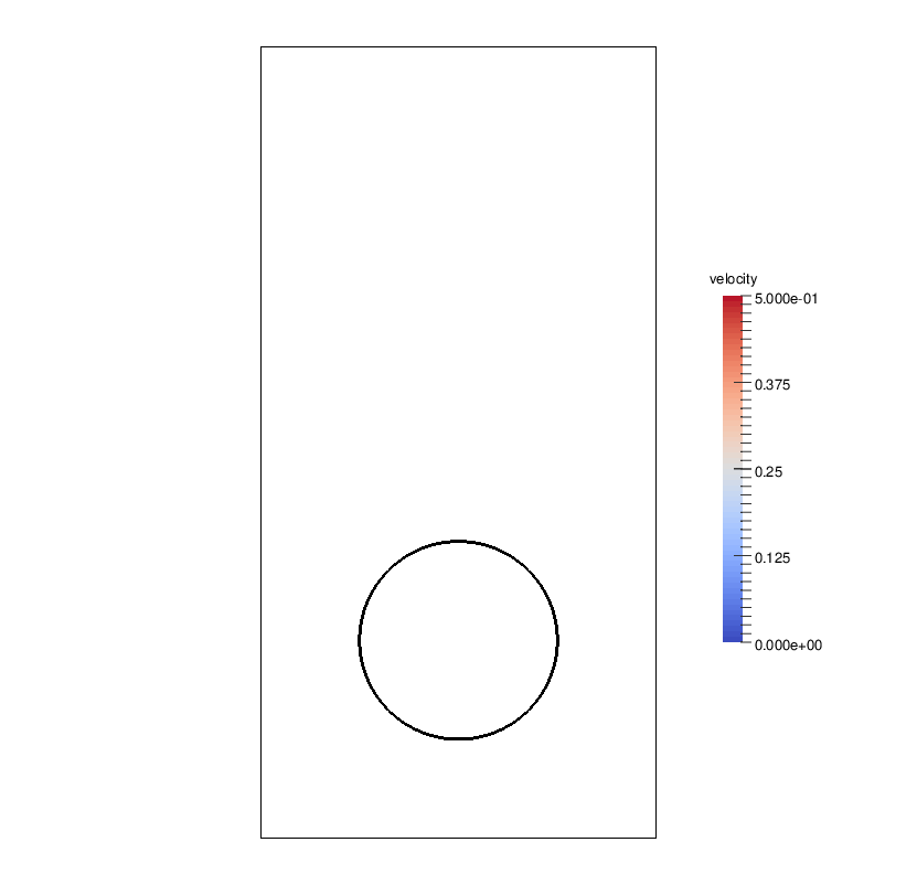
Let , for or be a given domain that contains two different immiscible, incompressible fluids (liquid-liquid or liquid-gas) which for all occupy time dependent regions and and which are separated by an interface , . We limit ourselves to interfaces formed by closed hypersurfaces, see Figure 1 for a pictorial representation in the case .
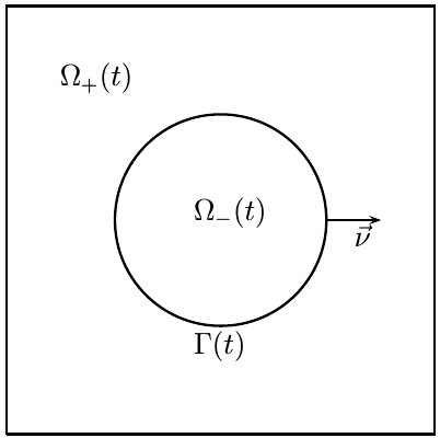
For later use, we assume that is a sufficiently smooth evolving hypersurface without boundary that is parametrized by , where is a given reference manifold such that . Then
| (2.1) |
defines the velocity of , and is the normal velocity of the evolving hypersurface , where is the unit normal on pointing into .
Denoting the velocity and pressure by and , respectively, we introduce the stress tensor
| (2.2) |
where , with , denotes the dynamic viscosities in the two phases, is the identity matrix and is the rate-of-deformation tensor. Here and throughout, denotes the characteristic function for a set .
The fluid dynamics in the bulk domain is governed by the two-phase Navier–Stokes model
| (2.3a) | |||||
| (2.3b) | |||||
where , with , denotes the fluid density in the two phases, and where is a possible forcing term. The velocity and stress tensor need to be coupled across the free surface . Viscosity of the fluids leads to the continuity condition
| (2.4) |
where denote the jump in velocity across the interface . Here and throughout, we employ the shorthand notation for a function ; and similarly for scalar and matrix-valued functions. The assumption that there is no change of phase leads to the dynamic interface condition
| (2.5) |
which means that the normal velocity of the interface needs to match the flow normal velocity across the interface . Moreover, the momentum conservation in a small material volume that intersects the interface leads to the stress balance condition
| (2.6) |
where is the interface stress tensor and is the surface divergence on . The operator is the surface gradient on and it is the orthogonal projection of the usual gradient operator on the tangent space of the surface . Therefore, given a smooth function defined on a neighbourhood of , it is defined as
| (2.7) |
with the usual projection operator defined as
| (2.8) |
It can be shown that the definition of does not depend on the chosen extension of , but only on the value of on . See e.g. [20, §2.1] for details. For later use, we also define the surface Laplacian, also known as Laplace–Beltrami operator, on as
| (2.9) |
We restrict ourselves to the case that the only force acting on the interface is the surface tension contact force. Therefore the interface stress tensor has the following constitutive equation
| (2.10) |
where is the surface tension coefficient. Substituting (2.10) in (2.6) we obtain, assuming is constant, the so called clean interface model for the interfacial forces
| (2.11) |
which, in the case of Newtonian stress tensor (2.2), assumes the form
| (2.12) |
Here denotes the mean curvature of , i.e. the sum of the principal curvatures of , where we have adopted the sign convention that is negative where is locally convex. In particular, see e.g. [20], it holds that
| (2.13) |
In order to close the system, we prescribe the initial data and the initial velocity . Finally, we impose the Dirichlet condition on and the free-slip condition and , , on , with denoting the outer unit normal of and . As usual, it holds that and . Therefore the total system of equations can be rewritten as follows:
| (2.14a) | |||||
| (2.14b) | |||||
| (2.14c) | |||||
| (2.14d) | |||||
| (2.14e) | |||||
| (2.14f) | |||||
| (2.14g) | |||||
In what follows we introduce different weak formulations for (2.14a–g), on which our finite element approximations will be based.
2.1 Eulerian weak formulations
In order to obtain a weak formulation for (2.14a–g), we define the function spaces, for a given ,
and let, as usual, and denote the –inner products on and , respectively. In addition, we let and denote the Lebesgue measure in and the -dimensional Hausdorff measure, respectively.
We also need a weak form of the differential geometry identity (2.13), which can be obtained by multiplying (2.13) with a test function and performing integration by parts leading to
| (2.15) |
Moreover, on noting (2.2) and (2.12), we have that
| (2.16) |
for all . Hence a standard weak formulation of (2.14a–g) is given as follows. Given and , for almost all find and such that
| (2.17a) | |||
| (2.17b) | |||
| (2.17c) | |||
| (2.17d) | |||
holds for almost all times . We notice that if is part of a solution to (2.14a–g), then so is for an arbitrary .
An alternative to the weak formulation (2.17a–d) can be obtained by following the paper [12]. These authors show that it is possible to derive an energy bound not only on the continuous level but also for a discretization based on this formulation. Due to the resulting structure of the equation, we will refer to this form as the antisymmetric weak formulation, and it is given as follows. Given and , for almost all find and such that
| (2.18) |
holds, together with (2.17b–d). For a derivation of (2.18) we refer to [12], see also [2].
2.2 ALE model and weak formulation
The Arbitrary Lagrangian Eulerian (ALE) technique consists in reformulating the time derivative by expressing it with respect to a fixed reference configuration. A special homeomorphic map, called the ALE map, associates, at each time , a point in the current computational domain to a point in the reference domain . Note that for convenience we consider the domain to be time-dependent, even though in our situation it is fixed.
We now reformulate the two-phase Navier–Stokes system (2.14a–g), which is expressed in terms of Eulerian coordinates , by rewriting the velocity time derivative with respect to the so called ALE coordinate . Analogously to what is done in a front tracking approach to parametrize the interface , we can define the fixed reference manifold and extend the map to parametrize as . This extended map clearly still satisfies , given that . Moreover, we let be partitioned as with .
Now, let be a function defined on the Eulerian frame. The corresponding function on the ALE frame is defined as
| (2.19) |
In order to compute the time derivative of (2.19) with respect to the ALE frame, using the chain rule, we have . Therefore it holds that . Finally, introducing the domain velocity
| (2.20) |
and the time derivative in the ALE frame
| (2.21) |
we obtain
| (2.22) |
The identity (2.22) is naturally extended to vector valued functions. We stress the fact that the domain velocity for the interface points is consistent with the interface velocity . Therefore it holds that . We also point out that the ALE mapping is somehow arbitrary, apart from the requirement of conforming to the evolution of the domain boundary. Indeed the map of the boundary of the reference domain has then to provide, at all , the boundary of the current configuration, with .
Using (2.22) in the momentum equation (2.14a), we can rewrite it as:
| (2.23) |
We can notice that, with respect to the original formulation, there is a convective-type term due to the domain movement and the time derivative is computed in the fixed reference frame . Moreover, contrary to the original system, not only the regions are time dependent but also the whole domain is time dependent.
Obviously, if the domain is fixed, the additional convective term is zero and the time derivative in the ALE frame coincides with the usual time derivative in the Eulerian frame. This means that corresponds to a pure Eulerian method, while corresponds to a fully Lagrangian scheme. In our case, since we have a fixed domain , the ALE formulation might not seem very useful. But, at the discrete level, we are concerned with the evolution of the discrete triangulated domains. Therefore the discrete ALE map describes the evolution of the grid during the domain movement. It is indeed at the discrete level that the advantage of the ALE formulation emerges, as in an ALE setting the time advancing scheme provides directly the evolution of the unknowns at mesh nodes and thus that of the degrees of freedom of the discrete solutions.
In order to define the ALE weak formulation, we need to use a different functional setting for the test functions with respect to the one used for the Eulerian weak formulations. The reason is that here it needs to be defined on the moving domain . Therefore we introduce the admissible spaces of test functions on the reference domain
for a given . Then, using the ALE mapping, we can define the admissible spaces of test functions on the moving domain by setting
Hence, the ALE weak formulation of (2.23), (2.14b–g) is given as follows. Given and , find and such that
| (2.24a) | |||
| (2.24b) | |||
and (2.17c,d) hold for almost all times . Here denotes the –inner products on .
3 Finite element approximations
3.1 Eulerian finite element approximations
We consider the partitioning , , of into uniform time steps , see [12]. Moreover, let , , be a regular partitioning of the domain into disjoint open simplices , . From now on, the domain which we consider is the polyhedral domain defined by the triangulation . On we define the finite element spaces
where denotes the space of polynomials of degree on . Moreover, is the space of piecewise constant functions on and let be the standard interpolation operator onto .
Let and be the finite element spaces we use for the approximation of velocity and pressure, and let . In this paper, we restrict ourselves to the choice P2–(P1+P0), i.e. we set and , but generalizations to other spaces are easily possible.
We consider a fitted finite element approximation for the evolution of the interface . Let be a -dimensional polyhedral surface approximating the closed surface , . Let denote the exterior of and let be the interior of , where we assume that has no self-intersections. Then , and the fitted nature of our method implies that
where and . Let denote the piecewise constant unit normal to such that points into . In addition, let and .
In order to define the parametric finite element spaces on , we assume that , where is a family of mutually disjoint open -simplices with vertices . Then we define , where is the space of scalar continuous piecewise linear functions on , with denoting the standard basis of . As usual, we parametrize the new surface over using a parametrization , so that . Moreover, let be the mass lumped inner product on defined as
| (3.1) |
where are the vertices of , and where we define the limit . We naturally extend (3.1) to vector valued functions. Finally, let denote the standard –inner product on .
Our fully discrete finite element approximations based on the standard weak formulation (2.17a–d) are given as follows. Here we consider an explicit and an implicit treatment of the convective term in the Navier–Stokes equation.
: Let , an approximation to , and be given. For , find such that
| (3.2a) | |||
| (3.2b) | |||
| (3.2c) | |||
| (3.2d) | |||
and set . Here we have defined , .
: Let , an approximation to , and be given. For , find such that
| (3.3) |
and (3.2b–d), and set . Since the convective term in (3.2a) is treated explicitly, the scheme is a linear scheme that leads to a coupled linear system of equations for the unknowns at each time level. On the other hand, in (3.3) the convective term is treated implicitly, and so is a nonlinear scheme that leads to a coupled nonlinear system of equations for the unknowns at each time level.
An alternative fully discrete finite element approximation is based on the formulation (2.18), (2.17b–d). In particular, we consider the following scheme.
: Let , an approximation to , and be given. For , find such that
| (3.4) |
and (3.2b–d), and set . We note that the scheme corresponds to [12, (4.6a–d)] in the setting of an unfitted finite element approximation. Similarly to [12, Theorem 4.1] it is then straightforward to show that there exists a unique solution to that fulfils an energy inequality. In the unfitted case this energy inequality leads to an overall stability result if the bulk mesh does not change. Of course, in the fitted case considered here this will never be the case, unless the interface is stationary. Nevertheless, it is of interest to see how the scheme performs in practice, compared to and .
Moreover, we remark that all three schemes, , and , share the equations (3.2d). Apart from defining the discrete curvature, the equations (3.2d) can also be viewed as a side constraint on the distribution of mesh points, see [8, 9] for further details. In particular, they lead to an implicit tangential motion of the vertices on the discrete interface, so that the vertices of will in general be very well distributed in practice. For example, in the case it is possible to prove an asymptotic equidistribution property, see [2, Theorem 5].
Finally, we stress that the three schemes , and , all feature at least one term containing the interpolated velocity , and so an interpolation of the old velocity onto the new mesh is necessary, see also §4.1.4 below. In order to avoid such an interpolation, we consider an ALE formulation next.
3.2 ALE finite element approximation
In order to derive our fully discrete ALE finite element approximation, we first introduce a semidiscrete continuous-in-time fitted finite element approximation of (2.24a–d). Let be a regular partitioning of the reference domain into disjoint open simplices , . From now on, the reference domain , which we consider, is the polyhedral domain defined by the triangulation . On we define the finite element spaces
as well as , the space of piecewise constant functions on .
Then, using the discrete ALE mapping , we can define the finite element spaces on the discretized moving domains by
Here maps each simplex with straight faces in to a simplex with straight faces belonging to the triangulation of the discretized moving domain . For later use, we let and denote the appropriate spaces for the discrete velocities and pressure. In addition, we also define the discrete domain velocity as
| (3.5) |
with denoting the standard basis of , and denoting the vertices of .
Given , a family of -dimensional polyhedral surfaces with unit normal pointing into , the exterior of , analogously to the fully discrete case discussed in the previous section, we introduce the piecewise linear finite element spaces and , with denoting the standard basis of the former. Hence for all and , where are the vertices of . We also notice that the discrete interface velocity defined as
| (3.6) |
see e.g. [11, (3.3)], is simply the trace of on . We also introduce the interior , and the –inner products and on and , respectively. Moreover, let be the mass lumped inner product on . Finally, we let , , where denotes the standard interpolation operator onto , and set and .
Then, given and , for find and such that
| (3.7a) | |||
| (3.7b) | |||
| (3.7c) | |||
| (3.7d) | |||
The semidiscrete continuous-in-time fitted finite element scheme (3.7a–d) is a system of ODEs. Indeed, on defining the appropriate time-dependent matrices and vectors, we can rewrite (3.7a–d) in algebraic form as
| (3.8a) | |||
| (3.8b) | |||
| (3.8c) | |||
| (3.8d) | |||
where , , and are the unknown vectors for the velocity, pressure, interface curvature and interface position, respectively. See [2, (6.15)] for details.
It is now straightforward to obtain a fully discrete finite element approximation of (3.8a–d), since the only missing part is the temporal discretization. On recalling the partitioning , , of , and on applying a semi-implicit Euler scheme to (3.8a–d), we obtain
| (3.9a) | |||
| (3.9b) | |||
| (3.9c) | |||
| (3.9d) | |||
where , are some fully discrete bulk mesh velocities which, starting from , induce a sequence of bulk meshes , , where is an approximation to .
Following [45], we now rewrite (3.9a–d) into a form that is common in the finite element literature. Firstly, let and . Now to ease the notation, we introduce the following convention. For a function defined on , we can immediately transport it to any other configuration , with , using the mapping . Hence, when we need to integrate on we will write simply instead of , and we will adopt the same notation used for the inner products. Then, our ALE finite element approximation (3.9a–d), which is based on the variational formulation (2.24a–d), can be written as follows.
: Let , , and be given. For , find such that and such that
| (3.10a) | |||
| (3.10b) | |||
and (3.2c,d), and set , as well as , where . Here we note that in practice the bulk mesh velocity will be obtained with the help of an iterative solution and smoothing procedure, see the next section for more details. Moreover, we recall that the side constraint (3.2d) will lead to a uniform distribution of the vertices on in the case , and to well distributed vertices in .
We stress that since the ALE formulation describes the evolution of the solution along trajectories, the velocity is defined on all the domains, and so in particular on and . Hence no interpolation of the velocity is necessary in the ALE formulation, unless a full bulk remeshing is performed because of severe mesh deformations. Finally we remark that at the discrete level, the domain often plays the role of the reference manifold, so that is never used in practice.
4 Solution methods
4.1 Eulerian schemes
In this subsection we discuss the solution methods and other implementation issues for the three Eulerian schemes , and .
4.1.1 Algebraic formulations
As is standard practice for the solution of linear systems arising from discretizations of Navier–Stokes equations, we avoid the complications of the constrained pressure space in practice by considering an overdetermined linear system with instead. For example, for the scheme we consider the system (3.2a–d) with replaced by . For non-zero Dirichlet boundary data this requires a correction term on the right hand side of (3.2b). In particular, we replace (3.2b) with
| (4.1) |
The linear system of equations arising at each time step of the scheme then can be formulated as: Find , where , such that
| (4.2) |
where here, in a slight abuse of notation, denote the coefficients of these finite element functions with respect to some chosen basis functions. Moreover, denotes the coefficients of with respect to the basis of . The definitions of the matrices and vectors in (4.2) directly follow from (3.2a,c,d), (4.1), and their exact definitions can be found in e.g. [2, §5.5]. Note that for the submatrices we have used the convention that the subscripts refer to the test and trial domains, respectively. A single subscript is used where the two domains are the same. Of course, the algebraic formulation of the linear scheme can also be stated in the form (4.2).
In order to solve the nonlinear scheme , we employ the following fixed point iteration. Let and be given. Let and fix . Then, for , find such that
| (4.3a) | |||
| (4.3b) | |||
| (4.3c) | |||
| (4.3d) | |||
and repeat the iteration until . Finally, set and . Clearly, (4.3a–d) is a linear system for the unknowns that is of the form (4.2).
Remark 1.
At times we will be interested in numerical simulations for non divergence-free solutions, in particular when considering our convergence experiments in §5.1. Here the condition (2.3b) is replaced by in . Clearly, this leads to an additional term on the right-hand side of the discrete continuity equation (3.2b). In particular, we have to replace (4.1) with
| (4.4) |
The same adjustment is made on the right-hand side of (4.3b). In addition, we observe that the weak formulation (2.18) needs to be suitably adjusted, with the additional term on the right-hand side of (2.18), see [2] for details. As a consequence, the term needs to be added to the right-hand side of (3.4) for the scheme .
4.1.2 Solvers for the linear (sub)problems
Following the authors’ approach in [3], see also [12, 10], for the solution of (4.2) we use a Schur complement approach that eliminates from (4.2), and then use an iterative solver for the remaining system in . This approach has the advantage that for the reduced system well-known solution methods for finite element discretizations for standard Navier–Stokes discretizations may be employed. The desired Schur complement can be obtained as follows. Let
| (4.5) |
be the interface condensed operator. Then (4.2) can be reduced to
| (4.6a) | ||||
| and | ||||
| (4.6b) | ||||
We notice that when the linear system (4.6a) becomes
| (4.7) |
which for and corresponds to a discretization of the one-phase Navier–Stokes problem. This system is well known and a classical way to solve it is to use a preconditioned GMRES iteration. Therefore, we solve (4.6a), which is a slight modification of (4.7), employing a preconditioned GMRES iterative solver. For the inverse we employ a sparse decomposition, which we obtain with the help of the sparse factorization package UMFPACK, see [18], in order to reuse the factorization. Having obtained from (4.6a), we solve (4.6b) for .
As preconditioner for (4.6a) we employ the standard Navier–Stokes matrix
| (4.8) |
recall (4.7). Of course, as the pressure in the Navier–Stokes problem (4.7) is only unique up to a constant, the block matrix (4.8) is singular. Hence, in order to efficiently apply the preconditioner (4.8) as part of an iterative solution method for (4.6a), one can either use a sparse factorization method as provided by SPQR, see [19]. Alternatively, the matrix (4.8) can be suitably doctored to make it invertible, and then a sparse factorization can be obtained with the help of UMFPACK, see [18], as usual. In practice we pursued the latter approach, as it proved to be slightly more efficient. We refer to [2, §4.6] for more details.
4.1.3 Mesh generation and smoothing
Given the initial polyhedral surface , we create a triangulation
of that is fitted to with the help of the
package Gmsh, see [33].
The mesh generation process is controlled by characteristic length
parameter, which describes the fineness of the resulting mesh.
Then, for , having computed the new interface , we
would like to obtain a bulk triangulation that is fitted to
, and ideally is close to . This is to avoid
unnecessary overhead from remeshing the domain completely.
To this end, we perform the following smoothing step on , which
is inspired by the method proposed in [29], see also
[31]. Having obtained from the solution of
(4.2), we solve the linear elasticity problem: Find a
displacement such that
| (4.9) |
In practice we approximate (4.9) with piecewise linear elements and solve the resulting system of linear equations with the UMPFACK package, see [18]. The obtained discrete variant of , at every vertex of the current bulk grid , then represents the variation in their position that we compute in order to obtain .
Occasionally the deformation of the mesh becomes too large, and so a complete remeshing of becomes necessary. In order to detect the need for a complete remeshing, we define the angle criterion
| (4.10) |
where is a fixed constant. Moreover, is the set of all the angles of the simplex , which can be computed as , , with the unitary normal to the simplex face . In practice we perform a full remeshing if the criterion (4.10) holds with . We stress that in all our numerical simulations we never need to remesh the interface itself.
4.1.4 Velocity interpolation
We notice that in the three Eulerian schemes , and , all feature at least one term containing the interpolated velocity . Here the interpolation operator is needed because the velocity , which has been computed at time level , is defined on . Therefore, at the next time level , the previous velocity needs to be interpolated on , which will in general be different from , in order to be used.
The interpolation routine simply consists in evaluating the discrete function in all the degrees of freedom of a piecewise quadratic function defined on . The efficiency of this computation hinges on quickly finding the element in the bulk triangulation that contains the coordinates of the degree of freedom on that is currently of interest. Of course, a naive linear looping over all elements in is highly inefficient. A simple optimization to this naive search consists in starting a guided search from the last correctly found element, in the hope that the degrees of freedom on are traversed in such a way, the successive points are close to each other. If the element does not contain the new point, then the guided search moves to the neighbouring element that is opposite the vertex with the largest distance to the new point. For a convex domain, this search is always well-defined. For nonconvex domains this guided search can be combined with a naive linear search whenever a boundary face is encountered in the local search for the next neighbour.
The last ingredient to our velocity interpolation algorithm is the traversal of the degrees of freedom on . Ideally we would like to have a continuous path of elements, which visits, only once, all the elements of . This ensures that successive degrees of freedom on the new mesh are spatially close, and so the local guided search for the next element of to visit is likely to be very short. Unfortunately, since we use unstructured meshes, such a path, in general, is difficult to construct. Hence, instead of explicitly constructing such a path, we create a fictitious background lattice that covers the domain . Then each element of is assigned to the point on the lattice that is closest to its barycentre. Depending on the size of the lattice, , multiple entities can be mapped to the same point on the lattice. Since the lattice is structured, it is straightforward to build a continuous path which visits all its points. For example, for a rectangular domain in 2d we can use a snaking path that traverses the lattice alternating left-to-right and right-to-left, see Figure 2.
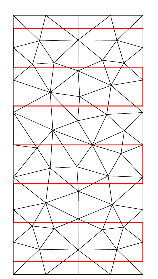
Now, in practice, the elements of are visited following the given lattice path. This means that, for each lattice point traversed, the associated entities on are visited. Clearly, for the algorithm to be efficient, the lattice size should be neither too small nor too large. In practice we use proportional to the characteristic length of the bulk mesh.
4.2 ALE scheme
The solution technique used to solve the ALE scheme is very similar to the one used to solve the nonlinear scheme , recall (4.3a–d), in that we use a fixed point iteration. However, the main difference is that at each time step for the ALE scheme we also find a bulk mesh velocity , and hence a new bulk mesh , as part of the solution process. More precisely, we find a solution for the scheme as follows. Let and be given. Set , , and fix . Then, for , find such that
| (4.11a) | |||
| (4.11b) | |||
| (4.11c) | |||
| (4.11d) | |||
Having obtained , the new bulk displacement is computed via the linear elasticity problem (4.9), see §4.1.3, and the new bulk mesh is updated accordingly. This iteration is repeated until and . Finally, set , and . Clearly, (4.11a–d) is once again a linear system of equations for the unknowns of the form (4.2).
Similarly to the Eulerian schemes, we monitor the mesh quality of the bulk meshes with the help of the criterion (4.10). In practice, if (4.10) holds with , then we perform a full remeshing of the domain , keeping fixed, and obtain the discrete velocity approximation on the new mesh via the procedure described in §4.1.4.
5 Numerical results
We implemented our numerical schemes within the DUNE framework,
using the FEM toolbox dune-fem, see
[14, 13, 21].
As grid manager we employed ALBERTA, [52],
and all the meshes were created with the library Gmsh,
[33]. All the schemes described in this paper are implemented as
a DUNE module called dune-navier-stokes-two-phase, available at
https://github.com/magnese/dune-navier-stokes-two-phase.
The simulations were performed as single thread computations on a cluster of
Xeon CPUs with frequency between 2.40GHz to 3.00GHz, and with at
least 16GB of memory.
5.1 Convergence experiments
Here we consider convergence experiments for exact solutions to the incompressible two-phase Navier–Stokes flow problem. These exact solutions will be characterised by expanding spheres. In particular, let be a sphere of radius , with curvature . Then, for , it can be shown that the expanding sphere with radius
| (5.1a) | |||
| together with | |||
| (5.1b) | |||
is an exact solution to the problem (2.14a–g), with (2.14b) replaced by
and with and on e.g. with .
A nontrivial divergence free and radially symmetric solution can be constructed on a domain that does not contain the origin. To this end, consider e.g. . Then, for , the expanding sphere with radius
| (5.2a) | |||
| together with | |||
| (5.2b) | |||
is an exact solution to the problem (2.14a–g) with and on .
For the following convergence tests, we choose the initial surface , and adaptive bulk meshes that use a finer resolution close to the interface. We compute the discrete solution over the time interval . We begin with the exact solution (5.1a,b) for on , with the physical parameters . Details on the discretization parameters are given in Table 1, where we also state the final number of bulk elements, , for the scheme . The values of for the remaining three schemes were very similar.
| (5.1a,b) | (5.2a,b) | ||||
|---|---|---|---|---|---|
| 32 | 296 | 310 | 460 | 216 | |
| 64 | 1 240 | 1 240 | 1 040 | 444 | |
| 128 | 4 836 | 4 836 | 2 628 | 1 378 | |
| 256 | 18 476 | 18 476 | 7 460 | 4 476 | |
We report on the computed errors in Table 2, where we have defined the error quantities , where , as well as , and . Moreover, we also define the estimated order of convergence EOC as , where and are the errors for the computations with characteristic lengths .
| EOC | EOC | CPU[s] | |||||
| 32 | 3.96456e-04 | 0 | - | 0 | 3.05157e-01 | - | 5 |
| 64 | 1.03429e-04 | 0 | - | 0 | 1.57053e-01 | 0.96 | 61 |
| 128 | 2.61302e-05 | 0 | - | 0 | 7.09596e-02 | 1.15 | 1 317 |
| 256 | 6.53463e-06 | 0 | - | 0 | 1.99794e-02 | 1.79 | 29 194 |
| 32 | 3.96456e-04 | 0 | - | 0 | 3.05157e-01 | - | 6 |
| 64 | 1.03429e-04 | 0 | - | 0 | 1.57053e-01 | 0.96 | 134 |
| 128 | 2.61302e-05 | 0 | - | 0 | 7.09596e-02 | 1.15 | 2 649 |
| 256 | 6.53463e-06 | 0 | - | 0 | 1.99794e-02 | 1.79 | 49 990 |
| 32 | 3.96456e-04 | 0 | - | 0 | 3.05157e-01 | - | 5 |
| 64 | 1.03429e-04 | 0 | - | 0 | 1.57053e-01 | 0.96 | 45 |
| 128 | 2.61302e-05 | 0 | - | 0 | 7.09596e-02 | 1.15 | 1 567 |
| 256 | 6.53463e-06 | 0 | - | 0 | 1.99794e-02 | 1.79 | 30 997 |
| 32 | 3.96823e-04 | 1.94467e-06 | - | 1.74315e-05 | 3.01900e-01 | - | 10 |
| 64 | 1.03462e-04 | 1.27547e-07 | 3.93 | 1.33117e-06 | 1.57054e-01 | 0.94 | 160 |
| 128 | 2.61390e-05 | 4.26296e-08 | 1.58 | 3.78211e-07 | 7.09597e-02 | 1.15 | 2 420 |
| 256 | 6.53680e-06 | 1.09827e-08 | 1.91 | 9.46271e-08 | 1.99793e-02 | 1.79 | 47 181 |
We observe from Table 2 that the schemes , and capture the velocity solution exactly. This is possible because the true velocity is linear, see (5.1b). We also notice that all the schemes capture the interface position with the same accuracy and exhibit similar errors for the pressure. In terms of the overall CPU times, we notice that the two linear schemes and , as well as the two nonlinear schemes and , have similar execution times, with the CPU times for the linear schemes lower than for the nonlinear schemes. Finally, we note that the number of full remeshings performed when was, depending on the scheme, between 1 and 4 while it was always 0 in all the other simulations for this test case.
In a second set of convergence experiments, we fix for the exact solution (5.2a,b) with and the physical parameters
We report on the errors of the exact solution (5.2a,b) in Table 3.
| EOC | EOC | CPU[s] | |||||
| 32 | 4.13976e-03 | 1.24661e-03 | - | 2.59441e-02 | 2.28403e-00 | - | 8 |
| 64 | 1.07627e-03 | 4.80240e-04 | 1.38 | 1.35253e-02 | 1.20439e-00 | 0.92 | 102 |
| 128 | 2.55529e-04 | 3.70025e-04 | 0.38 | 1.20309e-02 | 5.89258e-01 | 1.03 | 2 810 |
| 256 | 6.66480e-05 | 1.42910e-04 | 1.34 | 6.48222e-03 | 2.69953e-01 | 1.10 | 88 056 |
| 32 | 3.99899e-03 | 1.23928e-03 | - | 2.61424e-02 | 2.30983e-00 | - | 11 |
| 64 | 1.07657e-03 | 4.80445e-04 | 1.37 | 1.35256e-02 | 1.20449e-00 | 0.94 | 126 |
| 128 | 2.55562e-04 | 3.70165e-04 | 0.38 | 1.20325e-02 | 5.89236e-01 | 1.03 | 3 223 |
| 256 | 6.66478e-05 | 1.42914e-04 | 1.34 | 6.48232e-03 | 2.69982e-01 | 1.10 | 95 315 |
| 32 | 5.56564e-02 | 3.33673e-01 | - | 8.38557e-00 | 9.98404e+01 | - | 8 |
| 64 | 1.05282e-03 | 4.75502e-04 | 9.45 | 1.37127e-02 | 2.01792e+01 | 2.31 | 112 |
| 128 | 2.52742e-04 | 3.82170e-04 | 0.32 | 1.24067e-02 | 2.00690e+01 | 0.01 | 3 138 |
| 256 | 6.55951e-05 | 1.45885e-04 | 1.36 | 6.67192e-03 | 2.00294e+01 | 0 | 98 893 |
| 32 | 4.20717e-03 | 1.33379e-03 | - | 3.03240e-02 | 4.92318e-00 | - | 15 |
| 64 | 1.11280e-03 | 4.91358e-04 | 1.44 | 1.42754e-02 | 2.47229e-00 | 0.99 | 90 |
| 128 | 2.54196e-04 | 3.30194e-04 | 0.57 | 1.31294e-02 | 1.24058e-00 | 0.99 | 991 |
| 256 | 6.37496e-05 | 1.35898e-04 | 1.25 | 6.41819e-03 | 6.08051e-01 | 1.01 | 11 970 |
Firstly, we observe that the velocity and the interface position is captured with similar accuracy by all four schemes. However, we notice that the pressure error does not appear to converge for the scheme , which may be caused by the discontinuous jumps in density and viscosity. In addition, the scheme exhibits slightly higher pressure errors compared to and . We also note the vastly superior CPU times for the scheme compared to the other schemes. This is caused by the fact that the domain is nonconvex, and so we employ a simple linear search in our velocity interpolation routine, recall §4.1.4. Of course, the ALE scheme only needs to interpolate the velocity when a complete bulk remeshing is performed, and this leads to a significant reduction in the total simulation time. Finally, we note that the number of full remeshings performed during any simulation for this test case was always between 3 and 9.
5.2 Benchmark computations
Here we will present benchmark computations for the two rising bubble test cases proposed in [41, Table I]. To this end, we use the setup described in [41, Figure 2], which is with and . Moreover, the initial interface is . We also let and . For the discretization parameters, we choose , and nearly uniform bulk meshes.
We recall that the paper [41] used the proposed benchmarks to compare two different codes based on the level-set method with a direct front tracking ALE method, while the same benchmarks were used in [4, 32] to investigate different phase-field methods. Finally, in [12] an unfitted front tracking method was used for these benchmark problems.
5.2.1 Benchmark problem I
The physical parameters for the test case 1 in [41, Table I] are given by
| (5.3) |
We list our discretization parameters for this benchmark computation in Table 4, and report on the quantitative results for our four schemes in Table 5. Here we have defined the -component of the bubble’s centre of mass as , the degree of sphericity as , and the bubble’s rise velocity as .
| 32 | 2 210 | 1 816 | 1 816 | 1 794 | 1 820 |
| 64 | 8 822 | 7 544 | 7 156 | 7 490 | 7 566 |
| 128 | 35 092 | 29 276 | 29 014 | 28 968 | 28 296 |
| 0.8929 | 0.8975 | 0.9001 | 0.8925 | 0.8973 | 0.9004 | |
| 1.9040 | 1.9040 | 1.9170 | 2.0410 | 1.9120 | 1.9160 | |
| 0.2439 | 0.2424 | 0.2411 | 0.2439 | 0.2423 | 0.2410 | |
| 0.9350 | 0.9300 | 0.9180 | 0.9340 | 0.9300 | 0.9190 | |
| 1.0829 | 1.0852 | 1.0822 | 1.0820 | 1.0841 | 1.0819 | |
| CPU[s] | 10 236 | 29 610 | 234 396 | 17 771 | 72 837 | 403 904 |
| 0.8788 | 0.8851 | 0.8883 | 0.9013 | 0.9010 | 0.9030 | |
| 1.7920 | 1.7190 | 1.6790 | 1.9460 | 1.9050 | 1.8460 | |
| 0.2359 | 0.2344 | 0.2334 | 0.2435 | 0.2422 | 0.2410 | |
| 0.8860 | 0.8820 | 0.8750 | 0.9370 | 0.9330 | 0.9200 | |
| 1.0648 | 1.0622 | 1.0607 | 1.0877 | 1.0865 | 1.0824 | |
| CPU[s] | 5 887 | 19 703 | 146 538 | 13 628 | 63 136 | 351 867 |
We observe that the results in Table 5 are in very good agreement, except for the scheme . For this reason, we do not consider the scheme further in this section. The results for the remaining three schemes agree very well with the corresponding numbers from the finest discretization run of group 3 in [41], which are given by 0.9013, 1.9000, 0.2417, 0.9239 and 1.0817, and which are generally accepted as the most accurate in that paper. In fact, very similar results are also obtained in [12, Tables 2 and 3]. Moreover, we note that the number of full remeshings performed during any simulation for this test case was always between 2 and 4.
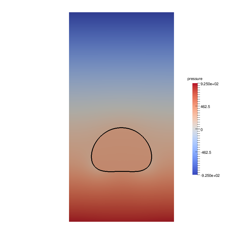
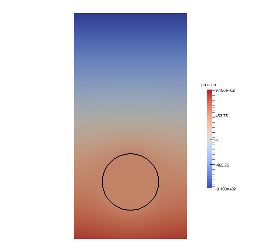
In Figure 3 we show the evolution of the discrete pressures for a simulation with interface elements using the scheme , while the velocities are visualized in Figure 4.


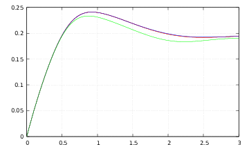
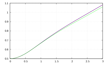
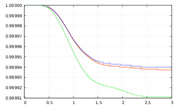
Finally, in Figures 5, 6, and 7 are reported, respectively, the evolution of the sphericity , rising velocity and barycentre over time. We notice almost identical results for the three schemes , and , which are in very good agreement with the plots shown in [41]. We also note the excellent area conservation shown in 8, where we visualize the evolution of the relative inner area over time.
5.2.2 Benchmark problem II
The physical parameters for the test case 2 in [41, Table I] are given by
| (5.4) |
We report on the quantitative results for this benchmark computation in Table 6, where we have used interface elements and initial bulk elements. The final number of bulk elements, , for the schemes , and was 10 638, 10 716 and 9 972, respectively.
| ( | |||
| 0.5435 | 0.5473 | 0.5266 | |
| 3.0000 | 3.0000 | 3.0000 | |
| 0.2503 | 0.2502 | 0.2502 | |
| 0.7290 | 0.7290 | 0.7300 | |
| 0.2403 | 0.2403 | 0.2400 | |
| 2.1070 | 2.1540 | 2.0670 | |
| 1.1383 | 1.1387 | 1.1385 | |
| CPU[s] | 132 498 | 236 635 | 236 253 |
We observe that the results in Table 6 are in good agreement with the corresponding numbers from the finest discretization run of group 3 in [41], which are given by 0.5144, 3.0000, 0.2502, 0.7317, 0.2393, 2.0600 and 1.1376. Here we note that there is little agreement on these results between the three groups in [41], but we believe the numbers of group 3 to be the most reliable ones. In fact, very similar results are also obtained in [12, Tables 5 and 6]. Moreover, we note that the number of full remeshings performed for this test case using the schemes , and was 787, 788 and 808, respectively. These large numbers are caused by the strong deformation of the rising bubble, with the narrow tail structure leading to very elongated bulk elements. In fact, until time only 6 remeshings are needed for each of the three schemes.
It is interesting to note that for this benchmark, the methods in [41] do not agree on whether the two tails of the rising bubble experience pinch-off of some droplets. But we note that the most accurate method there indicates that no pinch-off occurs, in agreement with our results and the results in [4, 12]. Of course, in a front tracking method like ours topological changes need to be performed heuristically when they occur, and this can be done, for example, as described in [17, 51].
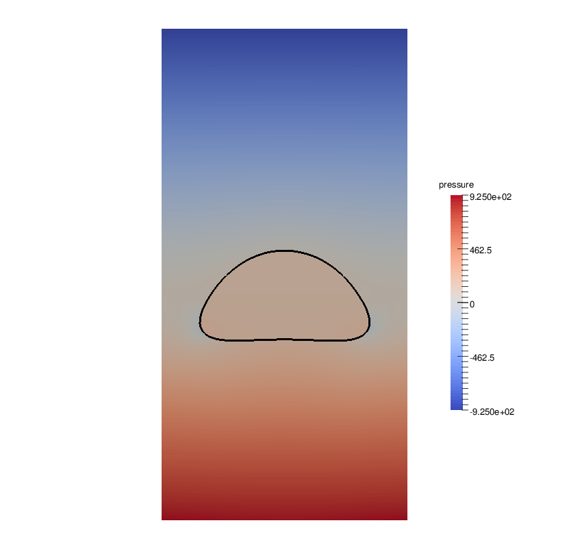
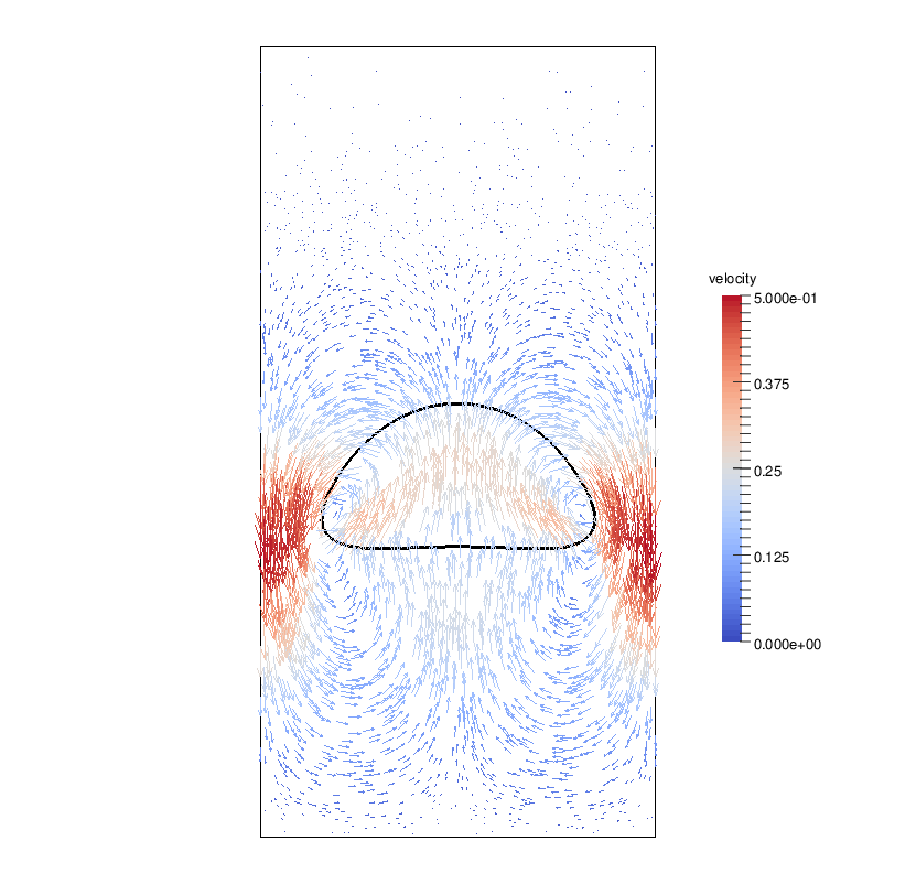
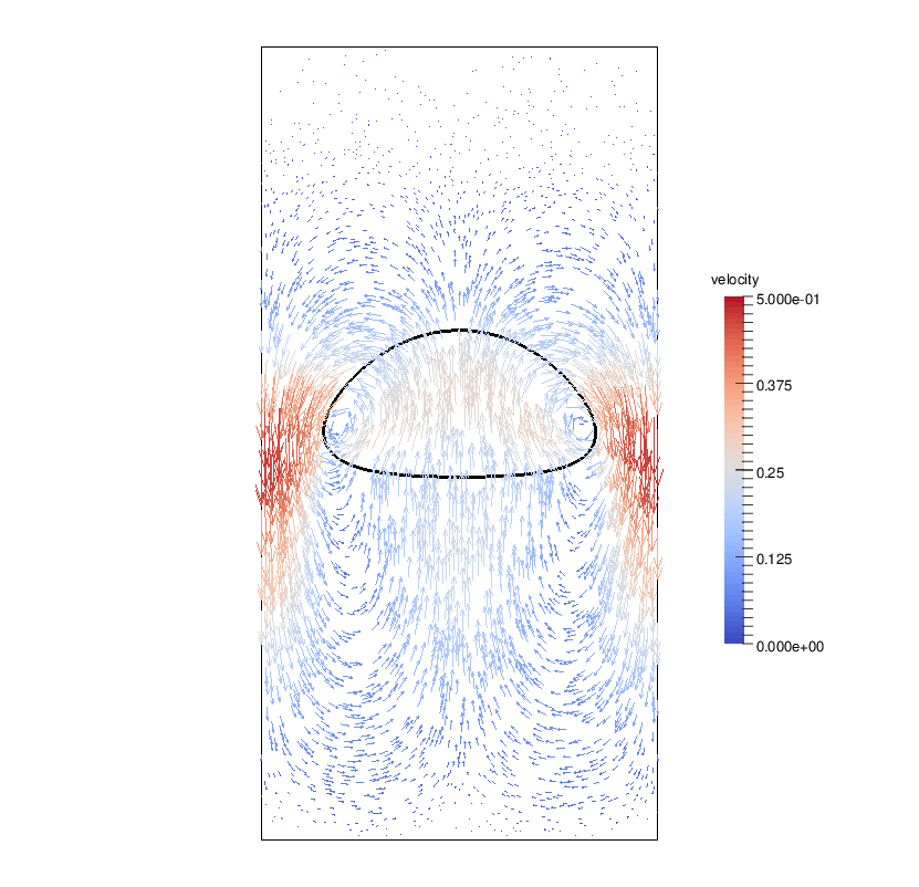
In Figure 9 we show the evolution of the discrete pressures for a simulation with interface elements using the scheme , while the velocities are visualized in Figure 10.

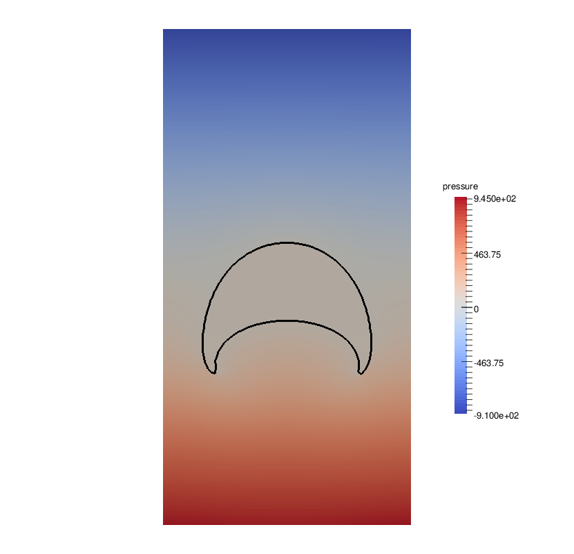
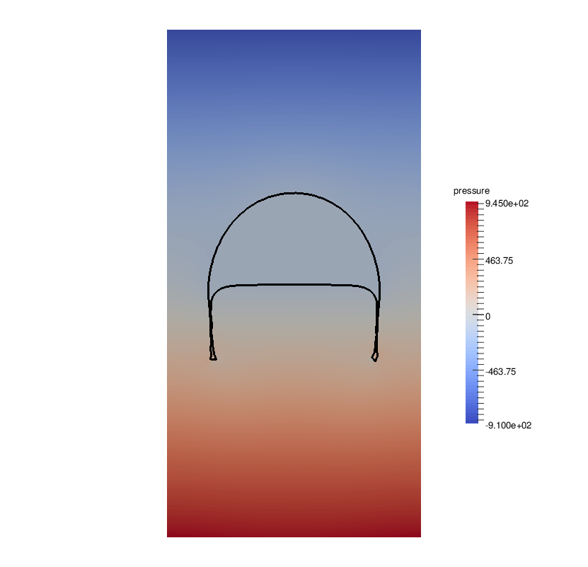
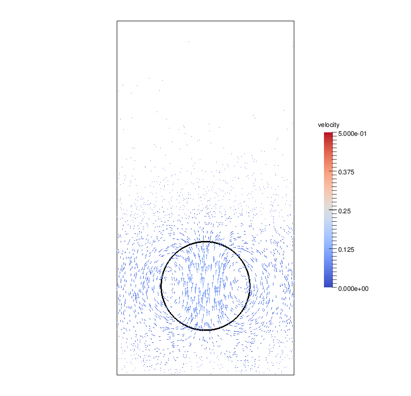
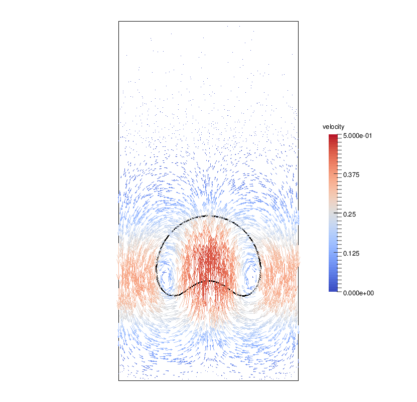
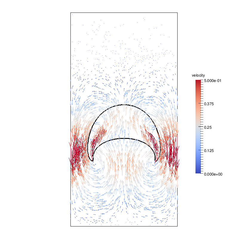
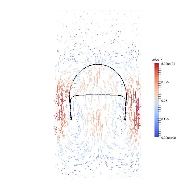
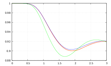
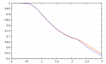
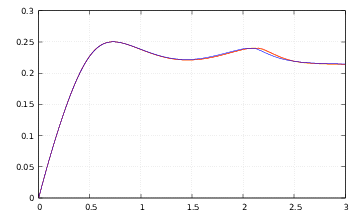
As before we show plots of the sphericity , the rising velocity , the barycentre and the relative inner area over time in Figures 11, 12, 13 and 14, respectively. In the former three figures we note the good agreement with the plots shown in [41]. As regards the plot of the relative inner area in Figure 14, we observe oscillations in the relative inner area between and which are caused by the very thin filaments originating at the bottom of the rising bubble.
Conclusions
We have introduced three Eulerian and one ALE scheme for the fitted finite element approximation of two-phase Navier–Stokes flow. Computationally the main difference between the Eulerian schemes and the ALE scheme is that for the former a bulk mesh adjustment needs to be performed after every time step, since the interface mesh in general moves, and so the fitted bulk mesh needs to be adjusted. Here we employ a bulk mesh smoothing procedure based on a linear elasticity problem. The mesh smoothing necessitates the interpolation of the discrete velocity approximation onto the new bulk mesh. It is often thought that the interpolation errors introduced by this procedure, together with the additional computational effort for the calculation of the interpolation, makes ALE schemes vastly superior to standard Eulerian approximations. However, our numerical results do not bear this out. In particular, for the physical and discretization parameters that we consider, the Eulerian schemes and perform as well as the ALE scheme in most of our convergence tests and benchmark computations. We conjecture that this good performance of the Eulerian schemes is connected to the fact that all our schemes maintain the interface mesh quality throughout, and so the interface mesh, and the finite element information stored on it, is never heuristically adjusted, not even during a full bulk remeshing. Moreover, thanks to an efficient element-traversal algorithm, the additional computational effort needed for the velocity interpolation was only noticeable on nonconvex domains.
References
- [1] H. Abels, H. Garcke, and G. Grün, Thermodynamically consistent, frame indifferent diffuse interface models for incompressible two-phase flows with different densities, Math. Models Methods Appl. Sci., 22 (2012), p. 1150013.
- [2] M. Agnese, Front tracking finite element methods for two-phase Navier–Stokes flow, PhD thesis, Imperial College London, London, 2017.
- [3] M. Agnese and R. Nürnberg, Fitted finite element discretization of two-phase Stokes flow, Internat. J. Numer. Methods Fluids, 82 (2016), pp. 709–729.
- [4] S. Aland and A. Voigt, Benchmark computations of diffuse interface models for two-dimensional bubble dynamics, Internat. J. Numer. Methods Fluids, 69 (2012), pp. 747–761.
- [5] D. M. Anderson, G. B. McFadden, and A. A. Wheeler, Diffuse-interface methods in fluid mechanics, in Annual review of fluid mechanics, Vol. 30, Annual Reviews, Palo Alto, CA, 1998, pp. 139–165.
- [6] ’L. Baňas and R. Nürnberg, Numerical approximation of a non-smooth phase-field model for multicomponent incompressible flow, M2AN Math. Model. Numer. Anal., 51 (2017), pp. 1089–1117.
- [7] E. Bänsch, Finite element discretization of the Navier–Stokes equations with a free capillary surface, Numer. Math., 88 (2001), pp. 203–235.
- [8] J. W. Barrett, H. Garcke, and R. Nürnberg, A parametric finite element method for fourth order geometric evolution equations, J. Comput. Phys., 222 (2007), pp. 441–462.
- [9] , On the parametric finite element approximation of evolving hypersurfaces in , J. Comput. Phys., 227 (2008), pp. 4281–4307.
- [10] , Eliminating spurious velocities with a stable approximation of viscous incompressible two-phase Stokes flow, Comput. Methods Appl. Mech. Engrg., 267 (2013), pp. 511–530.
- [11] , On the stable numerical approximation of two-phase flow with insoluble surfactant, M2AN Math. Model. Numer. Anal., 49 (2015), pp. 421–458.
- [12] , A stable parametric finite element discretization of two-phase Navier–Stokes flow, J. Sci. Comp., 63 (2015), pp. 78–117.
- [13] P. Bastian, M. Blatt, A. Dedner, C. Engwer, R. Klöfkorn, R. Kornhuber, M. Ohlberger, and O. Sander, A Generic Grid Interface for Parallel and Adaptive Scientific Computing. Part II: Implementation and Tests in DUNE, Computing, 82 (2008), pp. 121–138.
- [14] P. Bastian, M. Blatt, A. Dedner, C. Engwer, R. Klöfkorn, M. Ohlberger, and O. Sander, A Generic Grid Interface for Parallel and Adaptive Scientific Computing. Part I: Abstract Framework, Computing, 82 (2008), pp. 103–119.
- [15] F. Boyer, A theoretical and numerical model for the study of incompressible mixture flows, Comput. & Fluids, 31 (2002), pp. 41–68.
- [16] F. Boyer and S. Minjeaud, Hierarchy of consistent -component Cahn–Hilliard systems, Math. Models Methods Appl. Sci., 24 (2014), pp. 2885–2928.
- [17] T. Brochu and R. Bridson, Robust topological operations for dynamic explicit surfaces, SIAM J. Sci. Comput., 31 (2009), pp. 2472–2493.
- [18] T. A. Davis, Algorithm 832: UMFPACK V4.3—an unsymmetric-pattern multifrontal method, ACM Trans. Math. Software, 30 (2004), pp. 196–199.
- [19] , Algorithm 915, SuiteSparseQR: Multifrontal multithreaded rank-revealing sparse QR factorization, ACM Trans. Math. Software, 38 (2011), pp. 1–22.
- [20] K. Deckelnick, G. Dziuk, and C. M. Elliott, Computation of geometric partial differential equations and mean curvature flow, Acta Numer., 14 (2005), pp. 139–232.
- [21] A. Dedner, R. Klöfkorn, M. Nolte, and M. Ohlberger, A Generic Interface for Parallel and Adaptive Scientific Computing: Abstraction Principles and the DUNE-FEM Module, Computing, 90 (2010), pp. 165–196.
- [22] H. Ding, P. D. Spelt, and C. Shu, Diffuse interface model for incompressible two-phase flows with large density ratios, J. Comput. Phys., 226 (2007), pp. 2078–2095.
- [23] J. Donea, Arbitrary Lagrangian Eulerian methods, Comput. Meth. Trans. Anal., 1 (1983).
- [24] S. Dong, An efficient algorithm for incompressible N-phase flows, J. Comput. Phys., 276 (2014), pp. 691–728.
- [25] , Physical formulation and numerical algorithm for simulating N immiscible incompressible fluids involving general order parameters, J. Comput. Phys., 283 (2015), pp. 98–128.
- [26] S. Elgeti and H. Sauerland, Deforming fluid domains within the finite element method: five mesh-based tracking methods in comparison, Arch. Comput. Methods Eng., 23 (2016), pp. 323–361.
- [27] X. Feng, Fully discrete finite element approximations of the Navier–Stokes–Cahn–Hilliard diffuse interface model for two-phase fluid flows, SIAM J. Numer. Anal., 44 (2006), pp. 1049–1072.
- [28] L. Formaggia and F. Nobile, Stability analysis of second-order time accurate schemes for ALE–FEM, Comput. Methods Appl. Mech. Engrg., 193 (2004), pp. 4097–4116.
- [29] S. Ganesan, Finite element methods on moving meshes for free surface and interface flows, PhD thesis, University Magdeburg, Magdeburg, Germany, 2006.
- [30] S. Ganesan, A. Hahn, K. Simon, and L. Tobiska, ALE-FEM for two-phase and free surface flows with surfactants, in Transport processes at fluidic interfaces, Adv. Math. Fluid Mech., Birkhäuser/Springer, Cham, 2017, pp. 5–31.
- [31] S. Ganesan and L. Tobiska, An accurate finite element scheme with moving meshes for computing 3D-axisymmetric interface flows, Internat. J. Numer. Methods Fluids, 57 (2008), pp. 119–138.
- [32] H. Garcke, M. Hinze, and C. Kahle, A stable and linear time discretization for a thermodynamically consistent model for two-phase incompressible flow, Appl. Numer. Math., 99 (2016), pp. 151–171.
- [33] C. Geuzaine and J.-F. Remacle, Gmsh: A 3-D finite element mesh generator with built-in pre- and post-processing facilities, Internat. J. Numer. Methods Engrg., 79 (2009), pp. 1309–1331.
- [34] S. Groß and A. Reusken, An extended pressure finite element space for two-phase incompressible flows with surface tension, J. Comput. Phys., 224 (2007), pp. 40–58.
- [35] , Numerical methods for two-phase incompressible flows, vol. 40 of Springer Series in Computational Mathematics, Springer-Verlag, Berlin, 2011.
- [36] G. Grün and F. Klingbeil, Two-phase flow with mass density contrast: Stable schemes for a thermodynamic consistent and frame-indifferent diffuse-interface model, J. Comput. Phys., 257 (2014), pp. 708–725.
- [37] A. Hahn, K. Held, and L. Tobiska, ALE-FEM for two-phase flows, PAMM. Proc. Appl. Math. Mech., 13 (2013), pp. 319–320.
- [38] C. W. Hirt and B. D. Nichols, Volume of fluid (VOF) method for the dynamics of free boundaries, J. Comput. Phys., 39 (1981), pp. 201–225.
- [39] P. C. Hohenberg and B. I. Halperin, Theory of dynamic critical phenomena, Rev. Mod. Phys., 49 (1977), pp. 435–479.
- [40] T. Hughes, W. Liu, and T. Zimmermann, Lagrangian-Eulerian finite element formulation for incompressible viscous flows, Comput. Methods Appl. Mech. Engrg., 29 (1981), pp. 329–349.
- [41] S. Hysing, S. Turek, D. Kuzmin, N. Parolini, E. Burman, S. Ganesan, and L. Tobiska, Quantitative benchmark computations of two-dimensional bubble dynamics, Internat. J. Numer. Methods Fluids, 60 (2009), pp. 1259–1288.
- [42] D. Kay, V. Styles, and R. Welford, Finite element approximation of a Cahn–Hilliard–Navier–Stokes system, Interfaces Free Bound., 10 (2008), pp. 15–43.
- [43] R. J. LeVeque and Z. Li, Immersed interface methods for Stokes flow with elastic boundaries or surface tension, SIAM J. Sci. Comput., 18 (1997), pp. 709–735.
- [44] J. Lowengrub and L. Truskinovsky, Quasi-incompressible Cahn–Hilliard fluids and topological transitions, R. Soc. Lond. Proc. Ser. A Math. Phys. Eng. Sci., 454 (1998), pp. 2617–2654.
- [45] F. Nobile, Numerical Approximation Of Fluid-Structure Interaction Problems With Application To Haemodynamics, PhD thesis, EPFL, Lausanne, 2001.
- [46] F. Nobile and L. Formaggia, A stability analysis for the arbitrary lagrangian: Eulerian formulation with finite elements, East-West J. Numer. Math., 7 (1999), pp. 105–132.
- [47] S. Osher and R. Fedkiw, Level Set Methods and Dynamic Implicit Surfaces, vol. 153 of Applied Mathematical Sciences, Springer-Verlag, New York, 2003.
- [48] C. S. Peskin, The immersed boundary method, Acta Numer., 11 (2002), pp. 479–517.
- [49] S. Popinet, An accurate adaptive solver for surface-tension-driven interfacial flows, J. Comput. Phys., 228 (2009), pp. 5838–5866.
- [50] Y. Renardy and M. Renardy, PROST: a parabolic reconstruction of surface tension for the volume-of-fluid method, J. Comput. Phys., 183 (2002), pp. 400–421.
- [51] A. Sacconi, Front-tracking finite element methods for a void electro-stress migration problem, PhD thesis, Imperial College London, London, UK, 2015.
- [52] A. Schmidt and K. G. Siebert, Design of Adaptive Finite Element Software: The Finite Element Toolbox ALBERTA, vol. 42 of Lecture Notes in Computational Science and Engineering, Springer-Verlag, Berlin, 2005.
- [53] J. A. Sethian, Level Set Methods and Fast Marching Methods, Cambridge University Press, Cambridge, 1999.
- [54] M. Sussman, P. Semereka, and S. Osher, A level set approach for computing solutions to incompressible two-phase flow, J. Comput. Phys., 114 (1994), pp. 146–159.
- [55] P. Sváček, On numerical approximation of incompresible fluid flow with free surface influenced by surface tension, EPJ Web Conf., 143 (2017), p. 02122.
- [56] G. Tryggvason, B. Bunner, A. Esmaeeli, D. Juric, N. Al-Rawahi, W. Tauber, J. Han, S. Nas, and Y.-J. Jan, A front-tracking method for the computations of multiphase flow, J. Comput. Phys., 169 (2001), pp. 708–759.
- [57] S. O. Unverdi and G. Tryggvason, A front-tracking method for viscous, incompressible multi-fluid flows, J. Comput. Phys., 100 (1992), pp. 25–37.