New Type of String Solutions with Long Range Forces

Abstract

We explore the formation and the evolution of the string network in the Abelian Higgs model with two complex scalar fields. A special feature of the model is that it possesses a global $U(1)$ symmetry in addition to the $U(1)$ gauge symmetry. Both symmetries are spontaneously broken by the vacuum expectation values of the two complex scalar fields. As we will show the dynamics of the string network is quite rich compared with that in the ordinary Abelian Higgs model with a single complex scalar field. In particular, we find a new type of string solutions in addition to the conventional Abrikosov-Nielsen-Olesen (local) string solution. We call this the uncompensated string. An isolated uncompensated string has a logarithmic divergent string tension as in the case of the global strings, although it is accompanied by a non-trivial gauge field configuration. We also perform classical lattice simulations in the $2+1$ dimensional spacetime, which confirms the formation of the uncompensated strings at the phase transition. We also find that most of the uncompensated strings evolve into the local strings at later time when the gauge charge of the scalar field with a smaller vacuum expectation value is larger than that of the scalar field with a larger vacuum expectation value.

I Introduction

Cosmic strings (also known as vortex solutions) are one-dimensional topological defects which appear in various contexts of particle physics and condensed matter physics. The simplest theoretical framework to describe the string (vortex) formation is the Abelian Higgs model, where the $U(1)$ gauge symmetry, $U(1)_{local}$, is spontaneously broken by a vacuum expectation value (VEV) of a complex scalar field. The string appearing in this model is called the Abrikosov-Nielsen-Olesen (ANO) string Nielsen and Olesen (1973). At the phase transition of the $U(1)_{local}$ breaking, the strings are formed and make up a web-like structure, so-called the string network (see $e.g.$ the textbook Vilenkin and Shellard (2000)). Numerical simulations have widely investigated the properties of the interactions and the evolution of the string network (see $e.g.$ Albrecht and Turok (1985, 1989); Bennett and Bouchet (1990); Allen and Shellard (1990); Vincent et al. (1997); Martins and Shellard (2006); Ringeval et al. (2007); Olum and Vanchurin (2007); Fraisse et al. (2008); Blanco-Pillado et al. (2011); Vincent et al. (1998); Moore et al. (2002); Bettencourt and Rivers (1995); Bettencourt et al. (1997); Salmi et al. (2008); Achucarro and de Putter (2006); Pen et al. (1997); Durrer et al. (1999); Yamaguchi et al. (1999, 2000); Yamaguchi (1999); Yamaguchi and Yokoyama (2002, 2003); Cui et al. (2008); Hiramatsu et al. (2013); Hindmarsh et al. (2019)).

In this paper, we discuss the formation and the evolution of the string network in the Abelian Higgs model with two complex scalar fields. In particular, we consider a model with an additional global $U(1)$ symmetry, $U(1)_{global}$. Such an additional global symmetry naturally arises when the ratio of the absolute $U(1)_{local}$ charges of the two complex scalar fields is larger than $3$ (or less than $1/3$). In this case, there is no gauge-invariant interaction term which breaks $U(1)_{global}$ at the renormalizable level, and hence, it emerges as an accidental symmetry. This class of models has been considered, for instance, in the context of the axion models where the Peccei-Quinn symmetry Peccei and Quinn (1977a, b); Weinberg (1978); Wilczek (1978) is protected by (abelian) gauge symmetries Lazarides and Shafi (1982); Barr et al. (1982); Choi and Kim (1985); Fukuda et al. (2017, 2018); Ibe et al. (2018) from the quantum gravity effects Hawking (1987); Lavrelashvili et al. (1987); Giddings and Strominger (1988); Coleman (1988); Gilbert (1989); Banks and Seiberg (2011). This type of models is also discussed in condensed matter physics to understand the physics of high-temperature superconductivity Lee et al. (2006).

As we will see, the dynamics of the string network is much richer compared with that in the ordinary Abelian Higgs model with a single complex scalar field. In particular, we observe the existence of a new type of string solutions in addition to the ANO (local) string. We call the new type of the string solutions, the “uncompensated” strings. Around an uncompensated string, the covariant derivatives of the complex scalar fields are not canceled by the gauge field configuration at the large distance from the core of the string. Accordingly, an isolated uncompensated string has a logarithmically divergent string tension as in the case of the global strings. In the early universe, those strings can be formed at the phase transition, where the divergence is cutoff by a typical distance between the strings of the order of the Hubble length. Our classical lattice simulations (in the $2+1$ spacetime dimensions) confirm the formation of the uncompensated strings at the phase transition.

As a characteristic feature of this system, the strings with winding numbers larger than $1$ appear ubiquitously. This feature should be contrasted with the string formation in the Abelian Higgs model with a single complex scalar field in which it is quite rare to have a cosmic string with a large winding number in the cosmological context. We also find that the uncompensated strings have long-range repulsive and attractive forces. With the long-range forces, we find that the uncompensated strings tend to combine into the local ANO strings in the evolution of the string network when the gauge charge of the scalar field with a smaller VEV is larger than that of the scalar field with a larger VEV.

The organization of the paper is as follows. In Sec. II, we discuss the static string solutions analytically. In Sec. III, we show the results of the classical lattice simulations of the formation and the evolution of the string network in the $2+1$ dimensional spacetime. In Sec. IV, we derive the long-range force between the uncompensated string and the global string in an analytical way. The final section is devoted to our conclusions and discussions.

II String Solutions in Abelian Higgs Model

In this section, we discuss the string solutions in the Abelian Higgs model with two charged scalar fields. We assume that both the scalar fields obtain non-vanishing VEVs. A specific feature of the model is that it possesses the $U(1)_{global}$ symmetry in addition to the $U(1)_{local}$ symmetry. We here discuss the static field configurations in an analytical way with the expansion of the universe being neglected.

II.1 Model

The action of the model is given by

$$S=-\int d^{4}x\,(\mathcal{L}_{\Phi}+\mathcal{L}_{A})\ ,$$ (1)

with the Lagrangian densities

$$\mathcal{L}_{\Phi} =(\mathscr{D}_{\mu}\phi_{1})^{*}\mathscr{D}^{\mu}\phi_{1}+(\mathscr{D}_{\mu}\phi_{2})^{*}\mathscr{D}^{\mu}\phi_{2}+V(\phi_{1},\phi_{2})\ ,$$ (2)

$$\mathcal{L}_{A} =\frac{1}{4}F_{\mu\nu}F^{\mu\nu}.$$ (3)

Here, $\phi_{n}$ $(n=1,2)$ denote the two complex scalar fields and

$$F_{\mu\nu}=\partial_{\mu}A_{\nu}-\partial_{\nu}A_{\mu}\ ,$$ (4)

is the field strength of the gauge field $A_{\mu}$ of the $U(1)_{local}$ symmetry. The covariant derivative is defined by

$$\mathscr{D}_{\mu}\phi_{n}:=\partial_{\mu}\phi_{n}-ieq_{n}A_{\mu}\phi_{n}\ ,$$ (5)

where $q_{n}$ is the charge of $\phi_{n}$, and $e$ is the gauge coupling constant. In what follows, we normalize $q_{1}$ and $q_{2}$ so that they are relatively prime integers without loosing generality.

The scalar potential is taken to be

$$V=\frac{\lambda_{1}}{4}(|\phi_{1}|^{2}-\eta_{1}^{2})^{2}+\frac{\lambda_{2}}{4}(|\phi_{2}|^{2}-\eta_{2}^{2})^{2}-\kappa(|\phi_{1}|^{2}-\eta_{1}^{2})(|\phi_{2}|^{2}-\eta_{2}^{2})\ ,$$ (6)

where $\lambda_{1,2}(>0)$ and $\kappa$ are real valued dimensionless coupling constants, and $\eta_{1,2}$ are real valued constants with a mass dimension. This potential possesses two $U(1)$ symmetries under the phase rotations of the two complex scalar fields. One of the linear combination of these symmetries is identified as the $U(1)_{local}$ gauge symmetry, while the other symmetry is a global $U(1)_{global}$ symmetry. The global $U(1)_{global}$ symmetry naturally appears as an accidental symmetry in the renormalizable theory when $|q_{1}|+|q_{2}|$ is larger than $4$.

We consider the case with $\lambda_{1}\lambda_{2}>4\kappa^{2}$. In this case, both the $U(1)$ symmetries are spontaneously broken by the VEVs Saffin (2005),

$$\langle\phi_{n}\rangle=\eta_{n}\ ,\quad(n=1,2)\ .$$ (7)

The Goldstone modes in this system are decomposed into the gauge-invariant Goldstone boson and the would-be Goldstone boson Fukuda et al. (2017, 2018). To see this, let us define the phase component fields $\tilde{a}_{n}$ $(n=1,2)$ by

$$\phi_{1}=\frac{1}{\sqrt{2}}f_{1}\,e^{i\tilde{a}_{1}/f_{1}}\ ,\quad\phi_{2}=\frac{1}{\sqrt{2}}f_{2}\,e^{i\tilde{a}_{2}/f_{2}}\ ,$$ (8)

where the decay constants are given by $f_{n}=\sqrt{2}\eta_{n}$. The domains of the phase component fields are given

$$\tilde{a}_{1}/f_{1}=[0,2\pi)\ ,\quad\tilde{a}_{2}/f_{2}=[0,2\pi)\ ,$$ (9)

respectively. The $U(1)_{local}$ gauge symmetry is realized by the shifts of $\tilde{a}_{n}$,

$$\tilde{a}_{1}/f_{1}\to\tilde{a}_{1}/f_{1}+q_{1}\alpha\ ,\quad\tilde{a}_{2}/f_{2}\to\tilde{a}_{2}/f_{2}+q_{2}\alpha\ ,$$ (10)

where $\alpha$ is a local parameter of the $U(1)_{local}$ transformation.

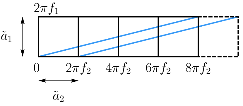
Figure 1: A gauge orbit for the $U(1)_{local}$ gauge symmetry for $(q_{1},q_{2})=(1,4)$ (blue lines). The orbit corresponds to the direction of the would-be Goldstone boson. The direction perpendicular to the blue lines corresponds to the gauge-invariant Goldstone boson. The domain of the gauge-invariant Goldstone boson is given by the interval between the blue lines.

The kinetic terms of $\tilde{a}_{n}$ are given by

$${\cal L} =|\mathscr{D}_{\mu}\phi_{1}|^{2}+|\mathscr{D}_{\mu}\phi_{2}|^{2}$$

$$=\frac{1}{2}(\partial\tilde{a}_{1})^{2}+\frac{1}{2}(\partial\tilde{a}_{2})^{2}-eA_{\mu}(q_{1}f_{1}\partial^{\mu}\tilde{a}_{1}+q_{2}f_{2}\partial^{\mu}\tilde{a}_{2})$$

$$-\frac{1}{2}e^{2}(q_{1}^{2}f^{2}_{1}+q_{2}^{2}f^{2}_{2})A_{\mu}^{2}$$

$$=\frac{1}{2}(\partial a)^{2}+\frac{1}{2}m_{A}^{2}\left(A_{\mu}-\frac{1}{m_{A}}\partial_{\mu}b\right)^{2}\ .$$ (11)

In the final expression, we use the Goldstone bosons defined by

$$\left(\begin{array}[]{cc}a\\ b\end{array}\right)=\frac{1}{\sqrt{q_{1}^{2}f^{2}_{1}+q_{2}^{2}f^{2}_{2}}}\left(\begin{array}[]{cc}q_{2}f_{2}&-q_{1}f_{1}\\ q_{1}f_{1}&q_{2}f_{2}\end{array}\right)\left(\begin{array}[]{cc}\tilde{a}_{1}\\ \tilde{a}_{2}\end{array}\right)\ .$$ (18)

The field $b$ is the would-be Goldstone boson which is absorbed by the $U(1)_{local}$ gauge boson in the unitary gauge. The mass of the gauge boson is given by,

$$m_{A}^{2}=e^{2}\left(q_{1}^{2}f^{2}_{1}+q_{2}^{2}f^{2}_{2}\right)$$ (19)

The field $a$ is the Nambu-Goldstone boson of the global $U(1)_{global}$ symmetry, which is invariant under the $U(1)_{local}$ symmetry (see Eq. (10)).

In Fig. 1, we show the gauge orbits of $U(1)_{local}$ for $(q_{1},~{}q_{2})=(1,~{}4)$ as the blue lines. As seen in the figure, the shift of $b$ from $0$ to $2\pi$ corresponds to the shift of $a_{1}$ from $0$ to $2\pi\,q_{1}$ and the shift of $a_{2}$ from $0$ to $2\pi\,q_{2}$. The direction perpendicular to the blue lines corresponds to the gauge-invariant Goldstone boson, $a$. The domain of $a$ is given by the interval between the blue lines,

$$a=[0,2\pi F_{a})\ ,\quad F_{a}=\frac{f_{1}f_{2}}{\sqrt{q^{2}_{1}f^{2}_{1}+q^{2}_{2}f^{2}_{2}}}\ .$$ (20)

II.2 Field Equations of the Static String Solutions

The Euler-Lagrange equations of $\phi_{n}$ and the gauge field are given by,

$$\mathscr{D}^{\mu}\mathscr{D}_{\mu}\phi_{n}=\frac{\partial V}{\partial\phi^{*}_{n}}\ ,$$ (21)

$$\partial_{\mu}F^{\mu\nu}={ie}\sum_{n=1}^{2}q_{n}\left[\phi^{*}_{n}\mathscr{D}^{\nu}\phi_{n}-(\mathscr{D}^{\nu}\phi_{n})^{*}\phi_{n}\right]\ .$$ (22)

Hereafter, we take the temporal gauge, $A_{0}=0$, which reduces the field equations to

$$\ddot{\phi}_{n}-\delta^{ij}\mathscr{D}_{i}\mathscr{D}_{j}\phi_{n}=-\frac{\partial V}{\partial\phi^{*}_{n}}\ ,$$ (23)

$$\ddot{A}_{k}-\delta^{ij}\partial_{i}F_{jk}={-ie}\sum_{n}^{2}q_{n}\left[\phi^{*}_{n}\mathscr{D}_{k}\phi_{n}-(\mathscr{D}_{k}\phi_{n})^{*}\phi_{n}\right],$$ (24)

and yields the constraint equation,

$$\delta^{ij}\partial_{i}\dot{A}_{j}=-ie\sum_{n=1}^{2}[\phi_{n}^{*}\dot{\phi}_{n}-\phi_{n}\dot{\phi}_{n}^{*}].$$ (25)

The dot denotes the time-derivative.

As an ansatz for the static string solutions, we assume

$$\phi_{1}(r,\theta) =\eta_{1}e^{in_{1}\theta}h_{1}(r)\ ,$$ (26)

$$\phi_{2}(r,\theta) =\eta_{2}e^{in_{2}\theta}h_{2}(r)\ ,$$ (27)

$$A_{\theta}(r) =\frac{1}{e}\xi(r)\ ,~{}A_{r}=A_{z}=0\ ,$$ (28)

in the cylindrical coordinate where $(r,~{}\theta,~{}z)$ is the radial distance, the azimuth angle, and the height, respectively. The integers $n_{1,2}$ denote the winding numbers of the strings consisting of $\phi_{1}$ and $\phi_{2}$, respectively.

Under the ansatz, the field equations in Eqs. (23) and (24) are reduced to

$$h_{1}^{\prime\prime}(R)+\frac{h_{1}^{\prime}(R)}{R}-{\beta}_{1}h_{1}(R)^{3}+\left({\beta}_{1}-\gamma_{2}\left(1-h_{2}(R)^{2}\right)-\frac{n_{1}^{2}}{R^{2}}\left(1-\frac{q_{1}}{n_{1}}\xi(R)\right)^{2}\right)h_{1}(R)=0\ ,$$ (29)

$$h_{2}^{\prime\prime}(R)+\frac{h_{2}^{\prime}(R)}{R}-{\beta}_{2}h_{2}(R)^{3}+\left({\beta}_{2}-\gamma_{1}\left(1-h_{1}(R)^{2}\right)-\frac{n_{2}^{2}}{R^{2}}\left(1-\frac{q_{2}}{n_{2}}\xi(R)\right)^{2}\right)h_{2}(R)=0\ ,$$ (30)

$$\xi^{\prime\prime}(R)-\frac{\xi^{\prime}(R)}{R}-2c_{1}\left(\xi(R)-\frac{n_{1}}{q_{1}}\right)h_{1}(R)^{2}-2c_{2}\left(\xi(R)-\frac{n_{2}}{q_{2}}\right)h_{2}(R)^{2}=0\ .$$ (31)

Here, we rescale the radial coordinate $r$ to $R$ by $R=r/r_{0}$ where

$$r_{0}=\frac{1}{e\sqrt{q_{1}^{2}\eta^{2}_{1}+q_{1}^{2}\eta^{2}_{2}}}\ .$$ (32)

The dash in the field equations denotes the derivative with respect to $R$. We also define

$$\beta_{n}=\frac{\lambda_{n}\eta^{2}_{n}}{2e^{2}\left({q_{1}^{2}\eta^{2}_{1}+q_{2}^{2}\eta^{2}_{2}}\right)}\ ,\quad\gamma_{n}=\frac{\kappa\,\eta^{2}_{n}}{e^{2}\left({q_{1}^{2}\eta^{2}_{1}+q_{2}^{2}\eta^{2}_{2}}\right)}\ ,\quad c_{n}=\frac{q_{n}^{2}\eta^{2}_{n}}{q_{1}^{2}\eta^{2}_{1}+q_{2}^{2}\eta^{2}_{2}}\ ,$$ (33)

for $n=1,2$.

II.3 Static String Solutions

To obtain the static string solutions, we consider the following boundary conditions,

$$h_{1}(R)=0\ ,~{}h_{2}(R)=0\ ,~{}\xi(R)=0\ ,$$ (34)

for $R\to 0$, and

$$h_{1}(R)=1\ ,~{}h_{2}(R)=1\ ,$$ (35)

for $R\to\infty$. Those boundary conditions are the same in the case of the static string solution of the Abelian Higgs model with one complex scalar field.

In the region of $R\to\infty$, $h_{1}(r)$ and $h_{2}(r)$ get close to unity, the field equation of $\xi$ in Eq. (31) becomes

$$\xi(R)^{\prime\prime}-\frac{\xi(R)^{\prime}}{R}-2\xi(R)+\frac{2c_{1}n_{1}}{q_{1}}+\frac{2c_{2}n_{2}}{q_{2}}=0\ ,$$ (36)

for $R\to\infty$. This field equation has an asymptotic solution,

$$\xi_{\infty}=\frac{c_{1}n_{1}}{q_{1}}+\frac{c_{2}n_{2}}{q_{2}}=\frac{n_{1}q_{1}\eta^{2}_{1}+n_{2}q_{2}\eta^{2}_{2}}{q_{1}^{2}\eta^{2}_{1}+q_{2}^{2}\eta^{2}_{2}}\ ,$$ (37)

and hence, the gauge field becomes

$$A_{\theta}=\frac{1}{e}\frac{n_{1}q_{1}\eta^{2}_{1}+n_{2}q_{2}\eta^{2}_{2}}{q_{1}^{2}\eta^{2}_{1}+q_{2}^{2}\eta^{2}_{2}}\ ,$$ (38)

for $R\to\infty$.

The asymptotic behaviors of the covariant derivatives of $\phi_{n}$ are then given by

$$\mathscr{D}_{\theta}\phi_{1} \to i\left(n_{1}-q_{1}\frac{n_{1}q_{1}\eta^{2}_{1}+n_{2}q_{2}\eta^{2}_{2}}{q_{1}^{2}\eta^{2}_{1}+q_{2}^{2}\eta^{2}_{2}}\right)\phi_{1}\ ,$$ (39)

$$\mathscr{D}_{\theta}\phi_{2} \to i\left(n_{2}-q_{2}\frac{n_{1}q_{1}\eta^{2}_{1}+n_{2}q_{2}\eta^{2}_{2}}{q_{1}^{2}\eta^{2}_{1}+q_{2}^{2}\eta^{2}_{2}}\right)\phi_{2}\ .$$ (40)

As the covariant derivatives contribute to the string tension via

$$\mu^{2}\sim 2\pi\int rdr\frac{1}{r^{2}}|\mathscr{D}_{\theta}\phi_{n}|^{2}\ ,$$ (41)

the string tension diverges at $r\to\infty$ unless both $\mathscr{D}_{\theta}\phi_{1}$ and $\mathscr{D}_{\theta}\phi_{2}$ vanish. Eqs. (39) and (40) show that this is possible only when the winding numbers satisfy,

$$n_{1}=N_{w}\times q_{1}\ ,\quad n_{2}=N_{w}\times q_{2}\ ,\quad N_{w}\in\mathbb{Z}\ .$$ (42)

The string solution which satisfies Eq. (42) has a finite string tension. The string solution which does not satisfy Eq. (42), on the other hand, has a logarithmically divergent tension as in the case of the global string. In the following, we call the former strings the compensated (local) strings, while the latter the uncompensated strings. It should be emphasized that the uncompensated strings are new-type of the string solutions which are absent in the conventional Abelian Higgs model with a single complex scalar field.

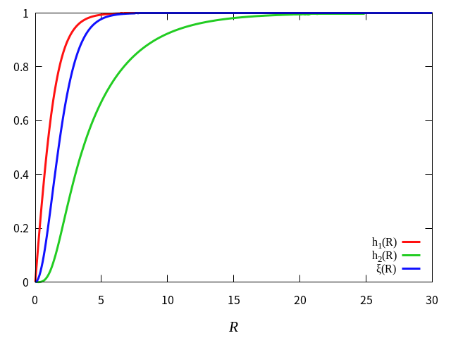
(a) $(n_{1},n_{2})=(1,4)$

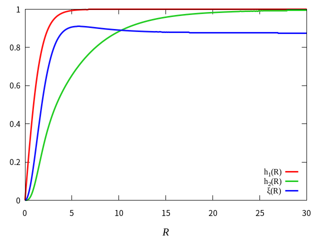
(b) $(n_{1},n_{2})=(1,3)$

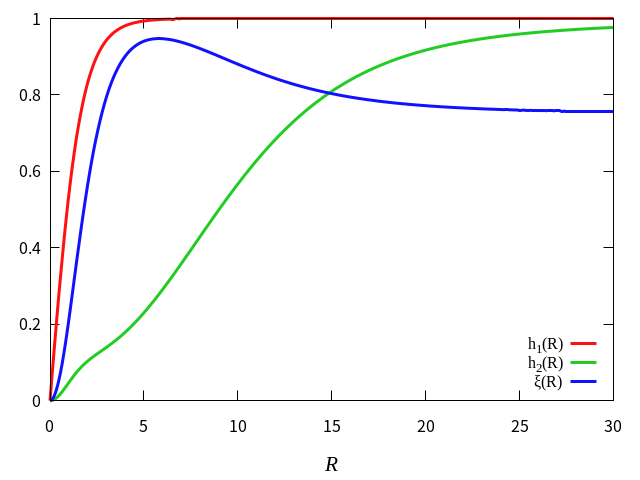
(c) $(n_{1},n_{2})=(1,2)$

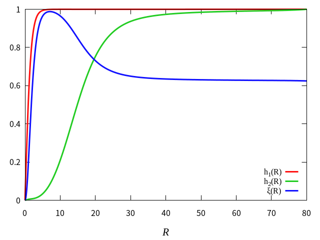
(d) $(n_{1},n_{2})=(1,1)$

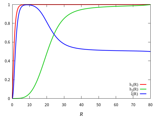
(e) $(n_{1},n_{2})=(1,0)$

Figure 2: The static string solutions as a function of $R$ for given winding numbers. In the figure, we take $q_{1}=1$ and $q_{2}=4$ and $\eta_{1}/\eta_{2}=4$. The upper-left panel corresponds to the compensated string for $N_{w}=1$. The other strings are uncompensated strings. Note that the figures in the first row are shown only up to $R\leq 30$ to emphases the structures around the string core, while those in the second row is up to $R\leq 80$.

To show examples of the string profiles in our model, we solve the equations (29)-(31) with the boundary conditions given in Eqs. (34)(35) and (37). We impose the asymptotic boundary conditions at $R=80$. In Fig. 2, we show the static string solutions for various values of $(n_{1},n_{2})$ in the case of $(q_{1},q_{2})=(1,4)$. We take other parameters as $e=1/\sqrt{2}$, $\eta_{1}/\eta_{2}=4$, $\lambda_{1,2}=1$, and $\kappa=0$. In the figure, only the upper-left panel corresponds to the compensated string with $N_{w}=1$. The other configurations are the uncompensated strings. The figure shows that the string core of $\phi_{2}$ becomes smaller for a larger $n_{2}$. The figure also shows the gauge field configuration converges to the asymptotic value in Eq. (38). We see that the gauge field configuration clings to the string solution of $\phi_{1}$ for a small $R$ and it converges to the asymptotic value at a large $R$.

The solution for $n_{2}=0$ requires an explanation. In this case, the condition, $h_{2}(r)=0$, at $R\to 0$ is not required and we assume the Neumann boundary condition for $h_{2}$. Even in this case, $h_{2}$ has a non-trivial configuration at around the string solution with $n_{1}\neq 0$ (see Eq. (30)).

In Fig. 3, we show how each type of the string solutions winds in the domain map of $(\tilde{a}_{1},\tilde{a}_{2})$ in the case of $(q_{1}=1,q_{2})=(1,4)$. The figure shows that the configuration of the compensated string, i.e. $(n_{1},n_{2})=(1,4)$, coincides with the orbit of the gauge transformation (see Fig. 1). The uncompensated strings, on the other hand, wind also in the direction of the gauge-invariant Goldstone boson. In fact, the string configuration with $(n_{1},n_{2})$ winds the Goldstone direction as

$$\frac{a}{F_{a}}=\left(q_{2}n_{1}-q_{1}n_{2}\right)\theta\ ,\quad\theta\in[0,2\pi)\ ,$$ (43)

which vanishes only for the compensated strings (see Eq. (18)).

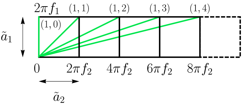
Figure 3: The string solutions in the domain map of $(\tilde{a}_{1},\tilde{a}_{2})$ for given $(n_{1},n_{2})$. The compensated string, $(1,4)$, corresponds to the direction of the orbit of the gauge transformation in Fig. 1. The uncompensated string winds not only in the direction of the would-be Goldstone boson but also in the gauge-invariant Goldstone direction.

III Classical Lattice Simulations

III.1 Preparation for Simulations

Here, let us summarize the setup of our numerical simulations. To take into account the cosmic expansion in the radiation dominated universe, we use the conformal time, $\tau$, with which the metric is given by,

$$ds^{2}=a^{2}(\tau)(-d\tau^{2}+d\boldsymbol{x}^{2})\ ,$$ (44)

where $a(\tau)$ is the scale factor. In the expanding universe, the field equations are modified to

$$\ddot{\phi}_{n}+2\mathcal{H}\dot{\phi}_{n}-\delta^{ij}\mathscr{D}_{i}\mathscr{D}_{j}\phi_{n}=-a^{2}V_{\phi^{*}_{n}}\ ,$$ (45)

$$\ddot{A}_{k}-\delta^{ij}\partial_{i}F_{jk}=-ia^{2}e\sum_{n}^{2}q_{n}\left[\phi^{*}_{n}\mathscr{D}_{k}\phi_{n}-(\mathscr{D}_{k}\phi_{n})^{*}\phi_{n}\right]\ ,$$ (46)

where $\mathcal{H}$ denotes the conformal Hubble parameter and the dot denotes the derivative with respect to the conformal time.

We also add the thermal mass term to the scalar potential

$$V_{\textrm{th}}=\frac{T^{2}}{12}\left(\lambda_{1}-\kappa+3e^{2}q^{2}_{1}\right)|\phi_{1}|^{2}+\frac{T^{2}}{12}\left(\lambda_{2}-\kappa+3e^{2}q^{2}_{2}\right)|\phi_{2}|^{2}\ .$$ (47)

The thermal mass term stabilizes the symmetry enhancement point, $\phi_{1,2}=0$, and hence, the $U(1)_{local}\times U(1)_{global}$ symmetry is restored at the high temperature, $T\gg\eta_{1,2}$.

Grid size	$1024^{2}$
Initial box size	$40H_{\rm in}^{-1}$
Final box size	$2H_{\rm fin}^{-1}$
Initial conformal time	$2.01\eta^{-1}_{1}$
Final conformal time	$40.2\eta^{-1}_{1}$
Time step	$1200$

Table 1: Simulation parameters. $H_{\rm in}$ and $H_{\rm fin}$ are the Hubble parameter at the initial time and the final time, respectively.

In the followings, we discuss the formation/evolution of the strings for,

$$(q_{1},~{}q_{2})=(1,~{}4)\ ,~{}(\eta_{1},~{}\eta_{2})=(1,~{}0.25)\ ,~{}\kappa=0\ ,\lambda_{1,2}=1\ ,e={\frac{1}{\sqrt{2}}}\ ,$$ (48)

as reference values. We also discuss the parameter dependencies at the end of this section. At the initial time, we impose the random values for $\phi_{i}(t_{\rm in},\boldsymbol{x})=\delta\phi(\boldsymbol{x})$ so that the distributions of the scalar fluctuations are given as the Planck distribution with the temperature $T=\sqrt{3}\eta_{1}$. Then we can determine $\dot{A}_{i}(t_{\rm in},\boldsymbol{x})$ by solving Eq. (25) with the Fourier transformation. At this stage, we can freely choose $A_{i}(t_{\rm in},\boldsymbol{x})$, so we simply assume $A_{i}(t_{\rm in},\boldsymbol{x})=0$. Throughout the simulations, we assume the radiation-dominant universe. We performed the simulations in a comoving box with periodic boundaries, and the time evolution is calculated by the Leap-Frog method and the spatial derivatives are approximated by the second-order finite difference. The simulation parameters are summarized in Table 1.

III.2 Formation of String Network

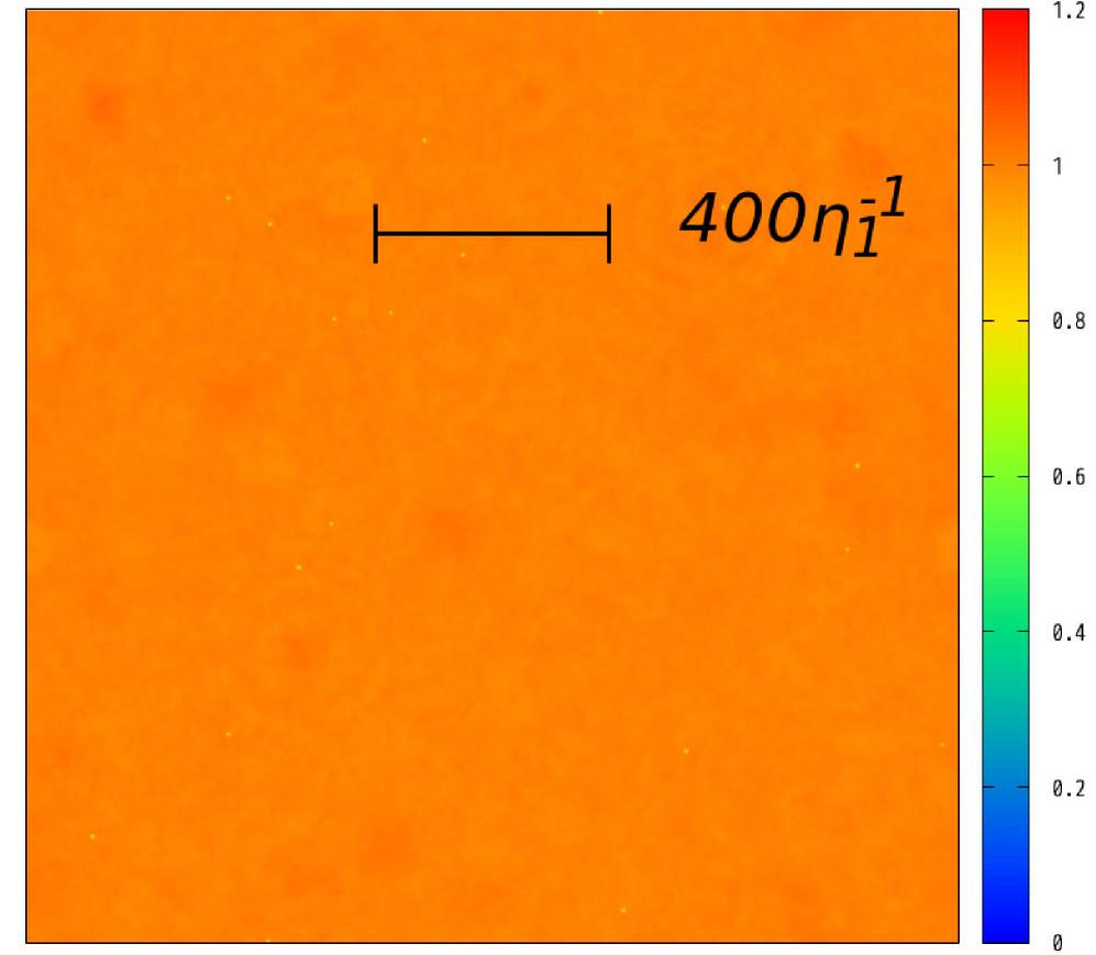
(a) $|\phi_{1}|$

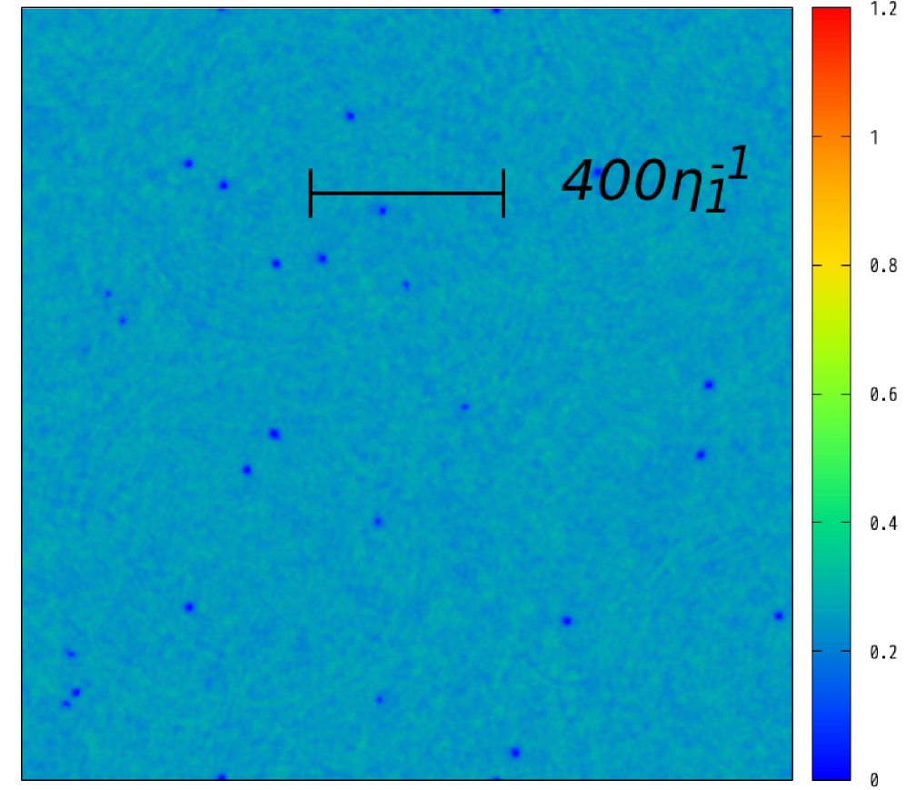
(b) $|\phi_{2}|$

(c) $\arg\phi_{1}$

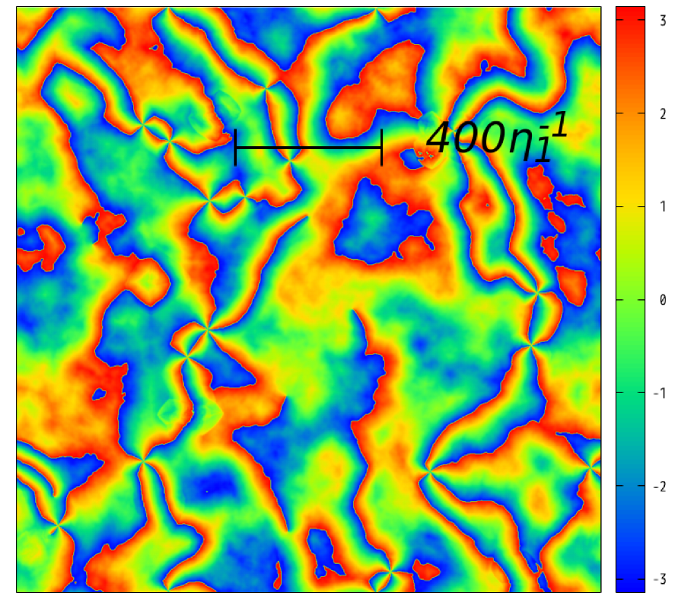
(d) $\arg\phi_{2}$

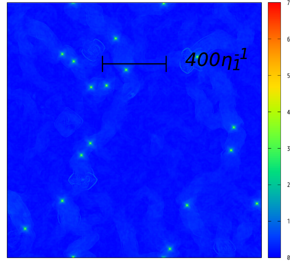
(e) $(A_{x},A_{y})$

—— Spot 1 $(n_{1},n_{2})=(1,4)$ ——
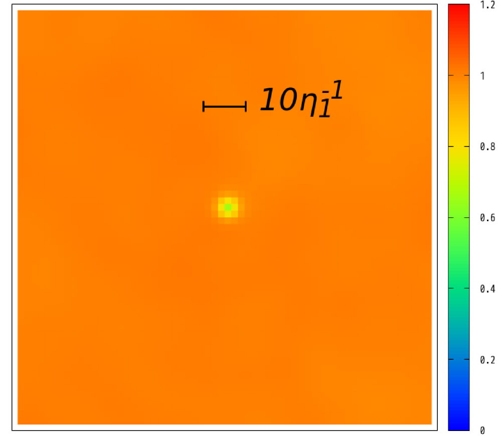
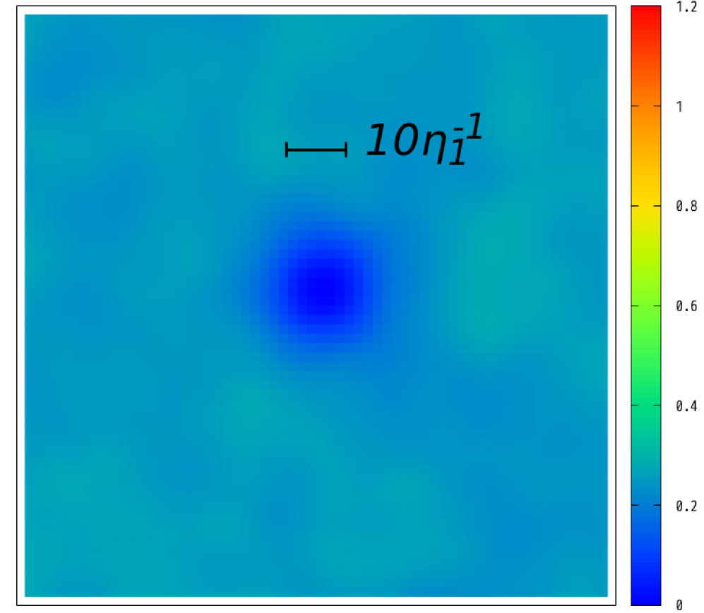
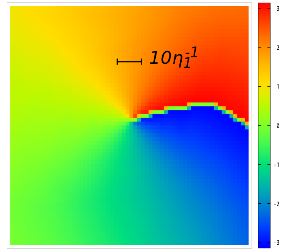
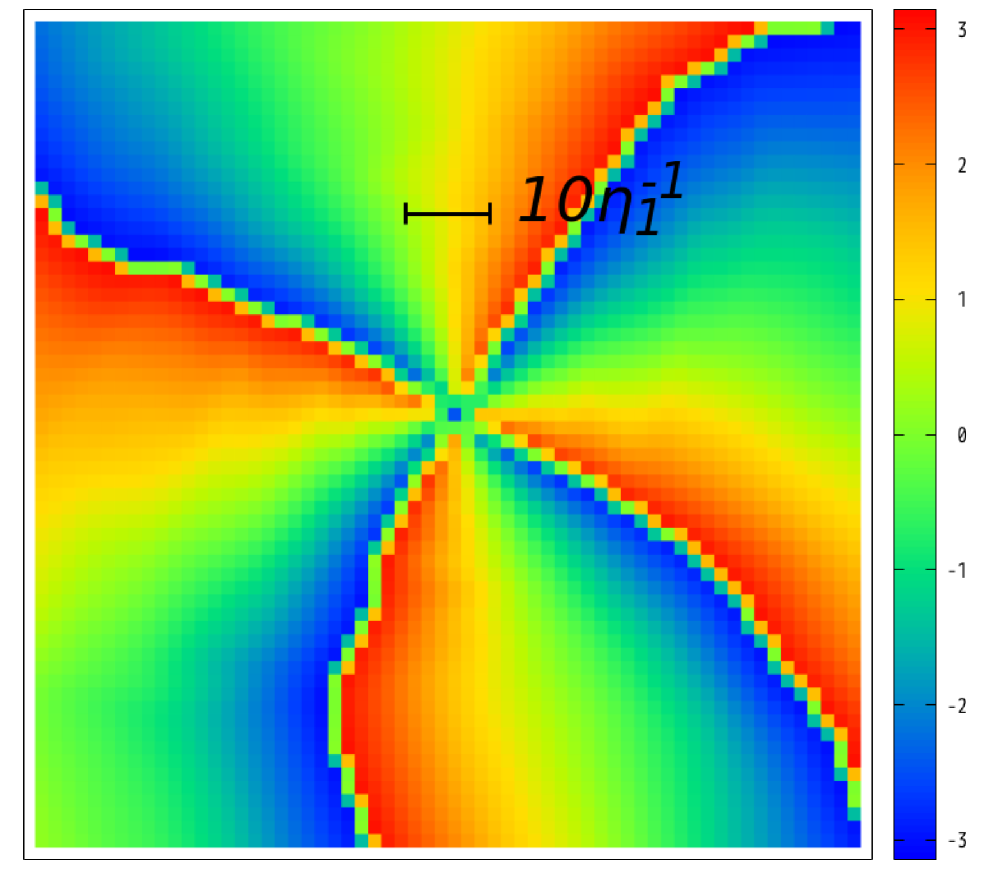
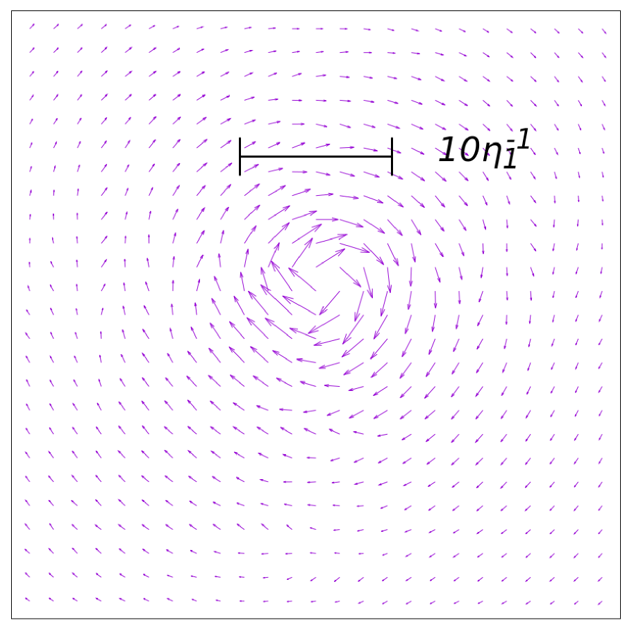
      —— Spot 2 $(n_{1},n_{2})=(1,3)$ ——
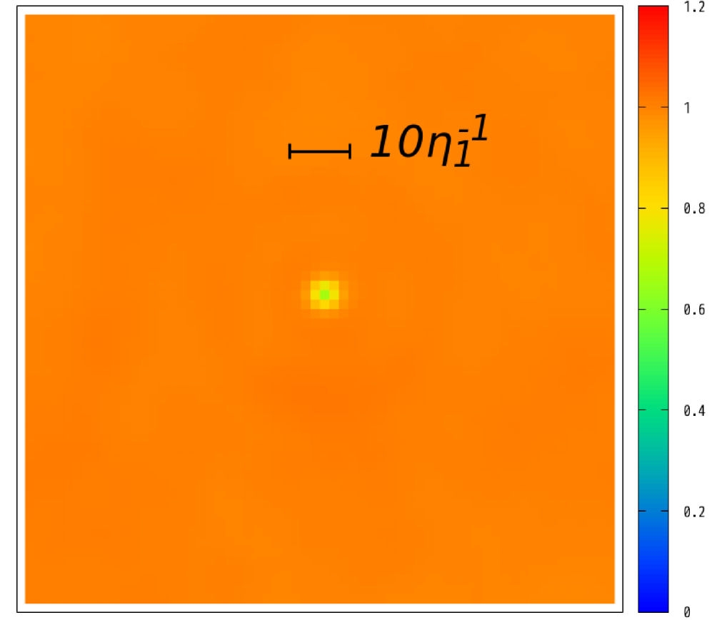
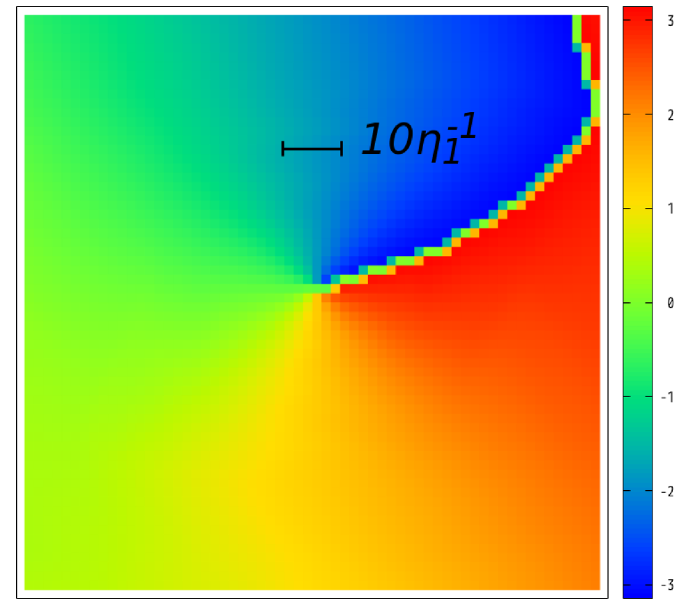
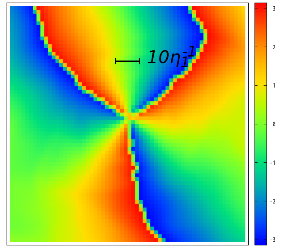
      —— Spot 3 $(n_{1},n_{2})=(1,5)$ ——
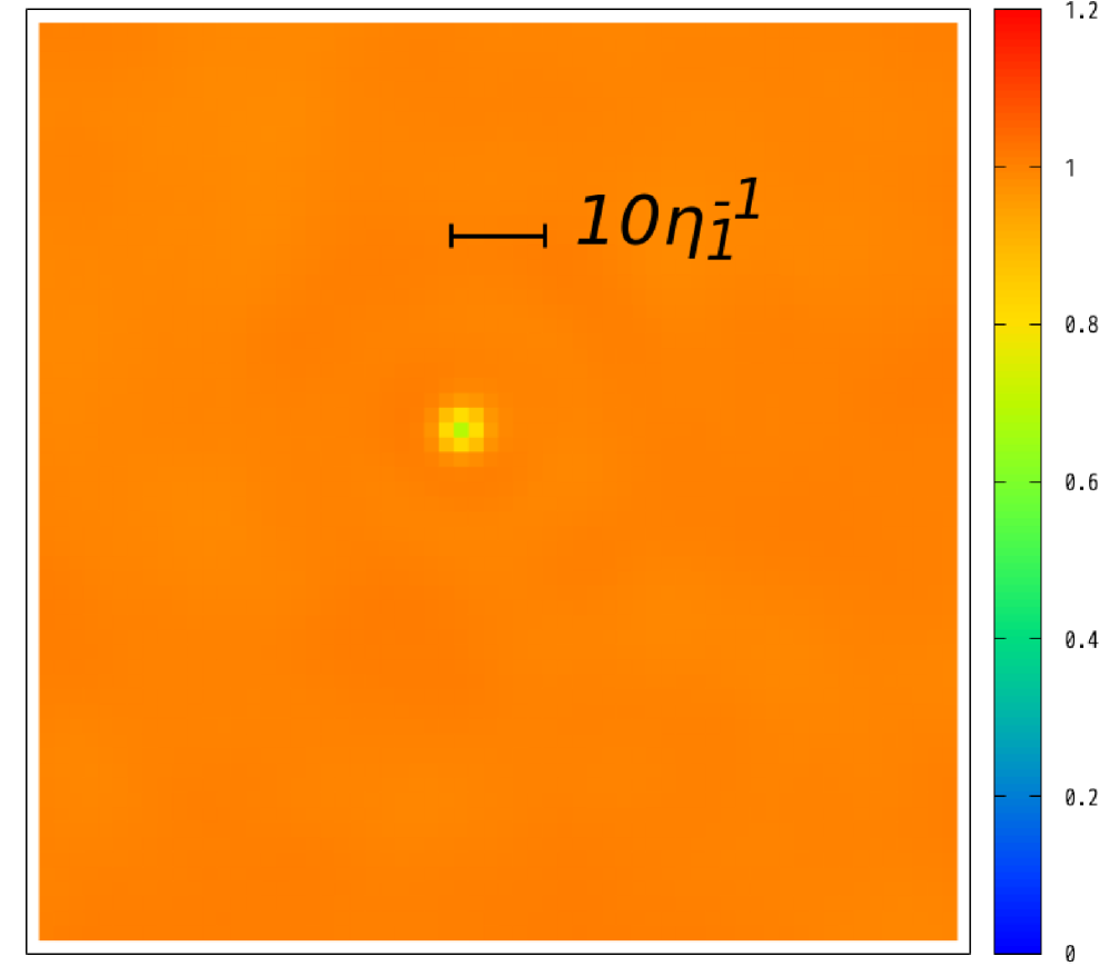
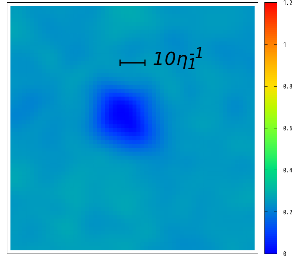
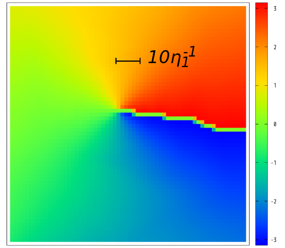
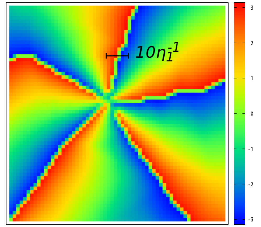
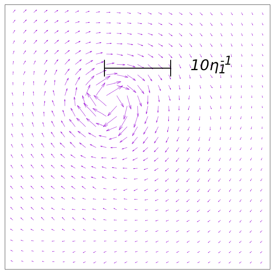
      —— Spot 4 $(n_{1},n_{2})=(0,1)$ ——
     

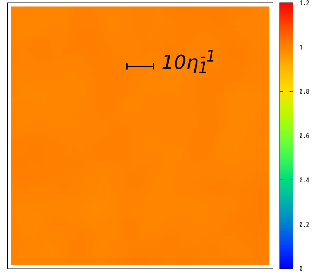
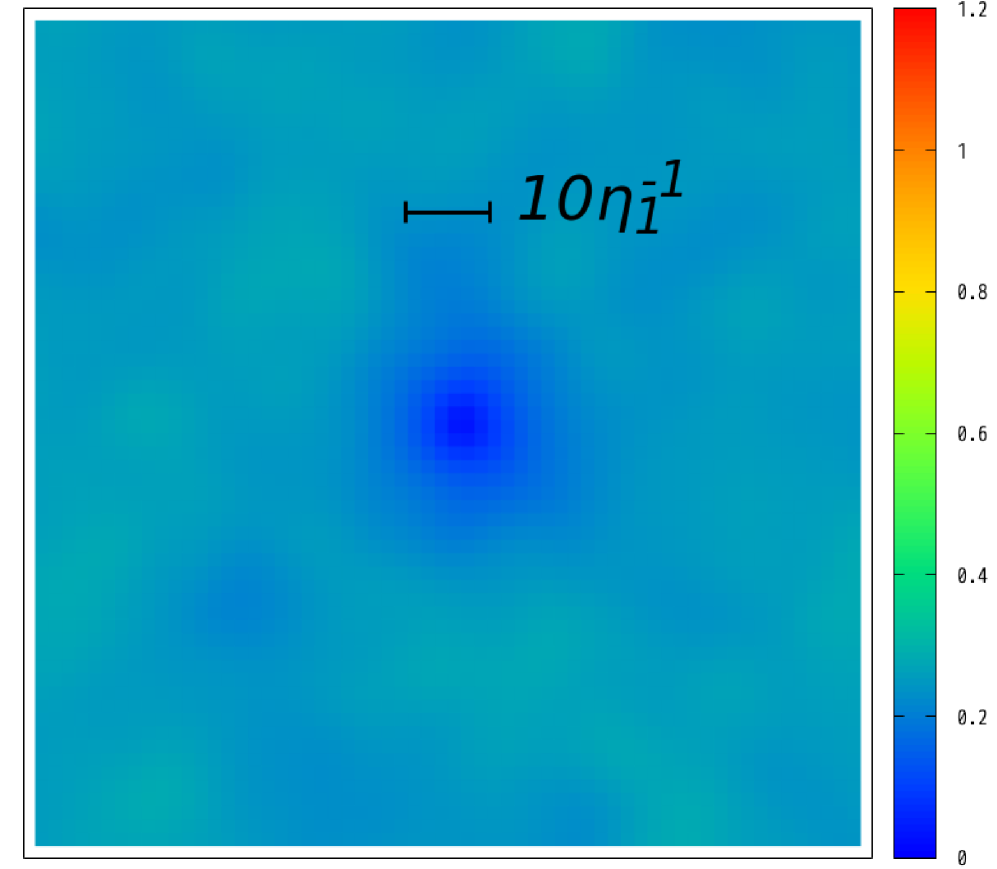
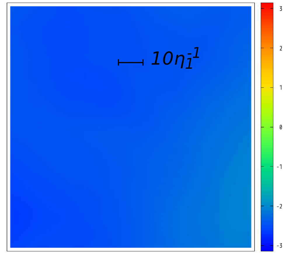
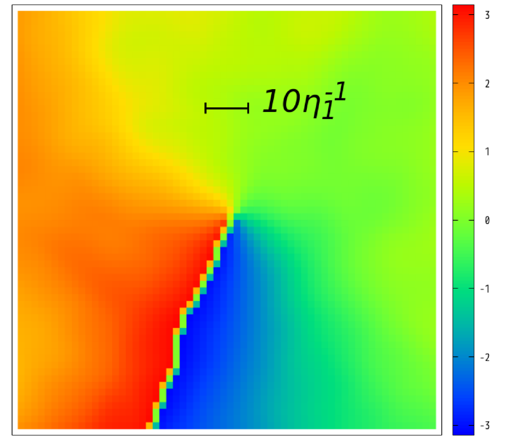
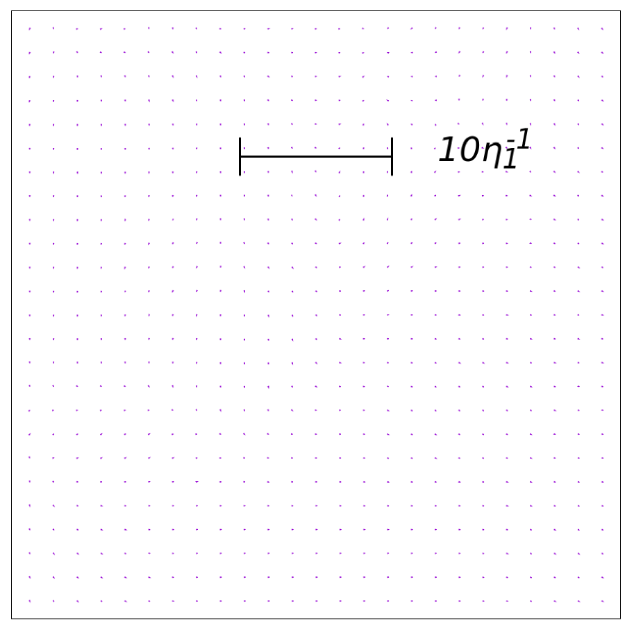
Figure 4: The field configurations in $2$-dimensional space after the phase transition. The first row shows the field configuration in the whole two-dimensional simulation box. The following rows are the closeups of the example spots with string configurations. The right panels show the amplitude of the gauge field in the whole simulation box (Top), and the gauge field in the $2$-dimensional space at each spot, whose amplitude is proportional to the length of the vector.

In Fig. 4, we show the field configurations in the $2$-dimensional space at the temperature, $T\ll\eta_{1,2}$, where the phase transition of the $U(1)$ symmetry breaking has completed. From the left, the figures show the absolute field values of $\phi_{1}$ and $\phi_{2}$ normalized by $\eta_{1}$, the phase distributions of $\phi_{1}$ and $\phi_{2}$, and the gauge field configurations. The first row shows the field configurations in the whole $2$-dimensional simulation box at the simulation end. At that time, the side length of the box is twice of the Hubble horizon length. The following rows are the closeups of the example spots with string configurations. The winding number of each spot is shown in the label.

The string configuration at the spot $1$ has the winding numbers, $(n_{1},n_{2})=(1,4)$. This configuration corresponds to the compensated (local) string (see Eq. (42)). As discussed in Sec. II, the non-trivial configuration of the gauge field cancels the covariant derivatives of the both complex scalars. The string configurations at the spots $2$ and $3$ are, on the other hand, the uncompensated strings. As emphasized in the previous section, they are the new-types of the string solutions in the present model. In these configurations, the covariant derivatives of the scalar fields are not canceled although they have non-trivial configurations of the gauge field around them. The string configuration at the spot $4$ has the winding number $(n_{1},n_{2})=(0,1)$. This corresponds to the global string which appears in the phase transition of the global $U(1)_{global}$ symmetry breaking. The global strings are not accompanied by non-trivial configurations of the gauge field.

In the present setup, we take $\eta_{1}/\eta_{2}=4$, and hence, the phase transition of the $U(1)_{local}\times U(1)_{global}$ breaking takes place in stages. At the first stage, the $U(1)_{local}$ breaking takes place at $T\sim\eta_{1}$. At the second stage, the $U(1)_{global}$ breaking takes place at $T\sim\eta_{2}$. At the first stage, the string configurations with $n_{1}\neq 0$ (mostly $n_{1}=1$) are formed in the similar manner to the original Abelian Higgs case. Then, around the string configurations with $n_{1}\neq 1$, $\phi_{2}$ also takes non-trivial configurations with various $n_{2}$ at the second stage. These configurations become either the compensated and the uncompensated strings. At the second stage, it is also possible that $\phi_{2}$ takes non-trivial configurations with $n_{2}\neq 0$ in the region where $\phi_{1}$ is trivial, i.e., $\langle\phi_{1}\rangle=\eta_{1}$. These configurations are the global strings, in which $\langle\phi_{1}\rangle=\eta_{1}$ is barely affected by the non-trivial configurations of $\phi_{2}$ due to the hierarchy $\eta_{1}\gg\eta_{2}$.

III.3 Evolution of String Network

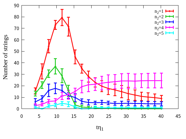
(a) Number of strings

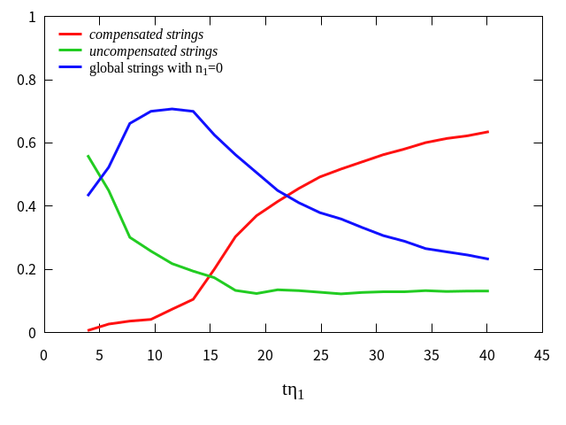
(b) $f_{\rm c},f_{\rm u}$ and $f_{\rm g}$

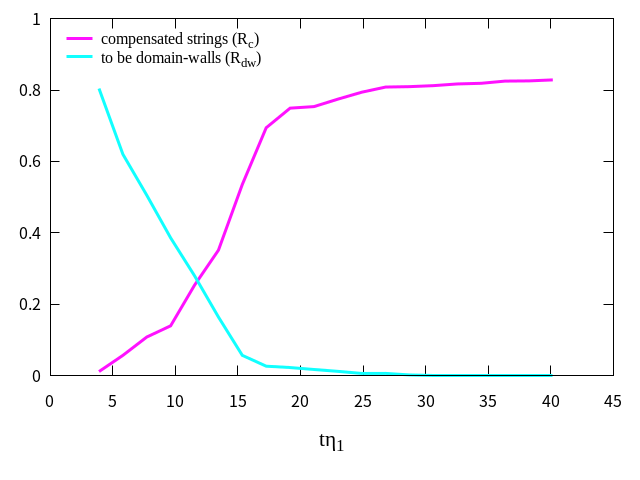
(c) $R_{\rm c}$, $R_{\rm dw}$

Figure 5: From left to right : The time evolution of the numbers of the strings with various $n_{2}$ in the computational domain; the number fractions of the compensated strings ($f_{\rm c}$), the uncompensated strings ($f_{\rm u}$), and the global strings ($f_{\rm g}$); and two kinds of number fractions ($R_{\rm c},R_{\rm dw}$) defined in Eqs. (49) and (50). The horizontal axis is the conformal time normalized by $\eta^{-1}_{1}$.

After the formation of the string configurations, the string network exhibits complicated evolution. In Fig. 5, we show the time evolution of the numbers of the strings with various $n_{2}$ in the computational domain. The results are obtained by averaging over 10 realizations, and the error bars show the statistical variance of the number of strings arising from the randomness of the initial conditions. To identify each string and compute its winding number for $\phi_{1}$ and $\phi_{2}$, we use the algorithm developed by Ref. Yamaguchi and Yokoyama (2003), and see also Ref. Hiramatsu et al. (2013). Throughout this paper, we regard two strings separated within $20\eta_{1}^{-1}$ as one string. We define $N_{c}$ as the number of compensated strings which have $(n_{1},n_{2})=(1,4)$, $N_{\rm u}$ as that of uncompensated strings with $n_{2}q_{1}-n_{1}q_{2}\neq 0$ with $n_{1}\neq 0$, $N_{{\rm g},1}$ as that of global strings with $(n_{1},n_{2})=(0,1)$, and $N_{{\rm g},>1}$ as that of global strings with $n_{1}=0$ and $n_{2}>1$. The total number of string, $N_{\rm tot}$, is given as $N_{\rm tot}=N_{\rm c}+N_{\rm u}+N_{{\rm g},1}+N_{{\rm g},>1}$. Note that in our simulations we observed no strings with $n_{1}>1$. We also show the evolution of the number fractions of the compensated strings, $f_{\rm c}=N_{\rm c}/N_{\rm tot}$ (red line), the uncompensated strings, $f_{\rm c}=N_{\rm u}/N_{\rm tot}$ (green line), and the global strings, $f_{\rm g}=(N_{{\rm g},1}+N_{{\rm g},>1})/N_{\rm tot}$ (blue line) in the middle panels. The right panels show the number ratio of the compensated strings to all the strings,

$$R_{\rm c}=\frac{N_{\rm c}}{N_{\rm c}+N_{\rm u}}\ ,$$ (49)

and the number ratio of the strings with $|n_{2}q_{1}-n_{1}q_{2}|>1$,

$$R_{\rm dw}=\frac{N_{|n_{2}q_{1}-n_{1}q_{2}|>1}}{N_{\mathrm{tot}}}\ .$$ (50)

Here, $R_{\rm dw}$ includes contributions both from the uncompensated and the global strings with $|n_{2}q_{1}-n_{1}q_{2}|>1$. This ratio is particularly important when the gauge-invariant Goldstone boson $a$ plays the role of the QCD axion. In fact, the so-called the axion domain wall number around the cosmic strings are given by (a multiple of) $|n_{2}q_{1}-n_{1}q_{2}|$, and the axion domain wall problem can be avoidable only for $|n_{2}q_{1}-n_{1}q_{2}|=0,1$, if we assume that the phase transition of the $U(1)$ symmetries take place after the end of inflation (see the Appendix A).

The figure shows that the number fraction of the compensated local strings increases in time, while those of the uncompensated and the global strings decrease. This means that the uncompensated strings and the global strings tend to combine together to form the compensated strings. After a while, the number of compensated strings tends to be converged, since the cosmic expansion separates the strings from each other and makes the compensation difficult. In Sec. IV, we discuss how the long-range force between the uncompensated and the global strings appears.

The simulation result in Fig. 5 also shows that the fraction of the compensated strings converges to a value smaller than $1$, and hence, there remain uncompensated/global strings at later times. We also found that $R_{\rm dw}\to 0$ in this simulation, which indicates that all the remaining strings in the network have the winding number either $0$ or $1$ in the gauge-invariant Goldstone direction. This result has important implications for the axion model building (see the Appendix. A).

In the simulation of Fig. 5, we do not include the thermal mass term in Eq. (47). Accordingly, the string formations of $\phi_{1}$ and $\phi_{2}$ take place simultaneously. In a realistic situation, however, the string formation of $\phi_{2}$ takes place much later than that of $\phi_{1}$. In Fig. 6, we show the same figures in Fig. 5 with the effects of the thermal mass in Eq. (47) taken into account. In this setup, the formation of the second string is delayed. Hence we performed the simulations with a larger box whose initial size is given by $80H_{\rm in}^{-1}$ and the grid size being $4096^{2}$. Even in this case, the winding number of most of strings is $n_{2}=4$ and thus they are compensated. So we can conclude that the string network at late time is not sensitive to the presence of the thermal effect. From now on, we do not take the thermal mass into account for the following simulations.

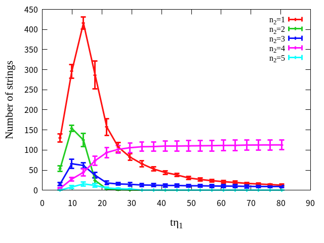
(a) Number of strings

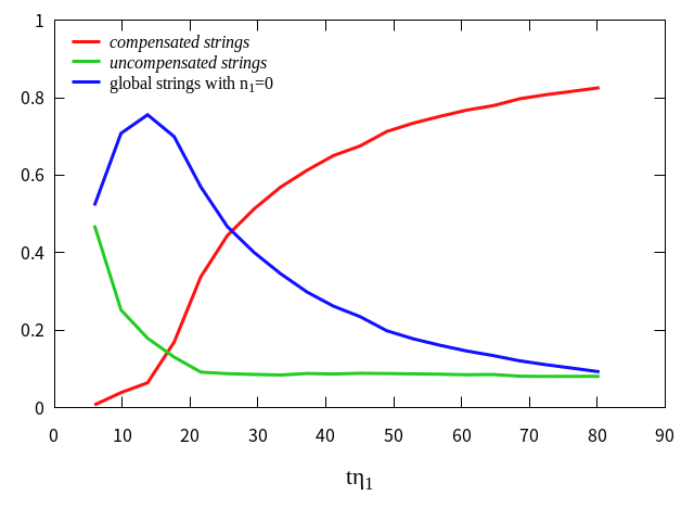
(b) $f_{\rm c},f_{\rm u}$ and $f_{\rm g}$

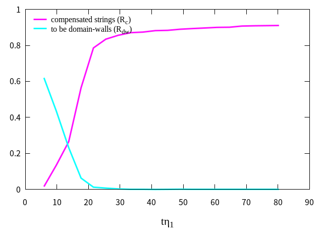
(c) $R_{\rm c}$, $R_{\rm dw}$

Figure 6: The same figures as that shown in Fig. 5 for the case including the thermal mass and $(q_{1},q_{2})=(1,4)$.

(a) Number of strings

(b) $f_{\rm c},f_{\rm u}$ and $f_{\rm g}$

(c) $R_{\rm c}$, $R_{\rm dw}$

—— $(q_{1},q_{2})=(1,1)$ ——

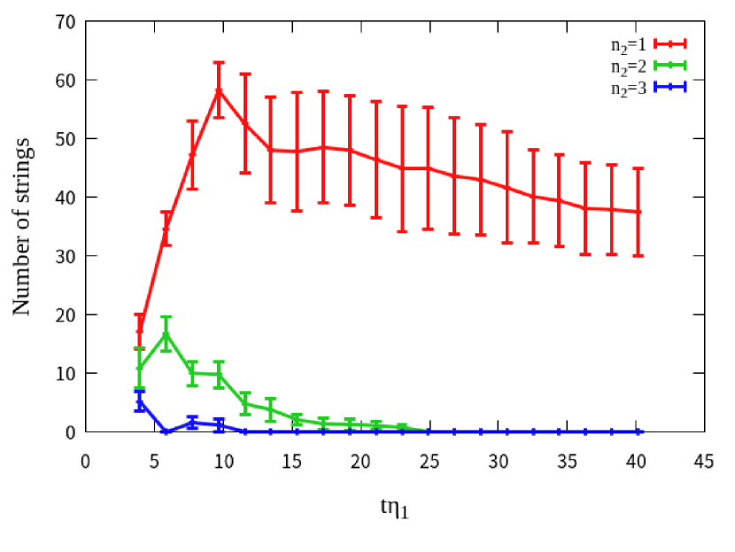
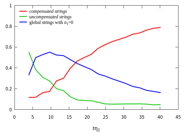
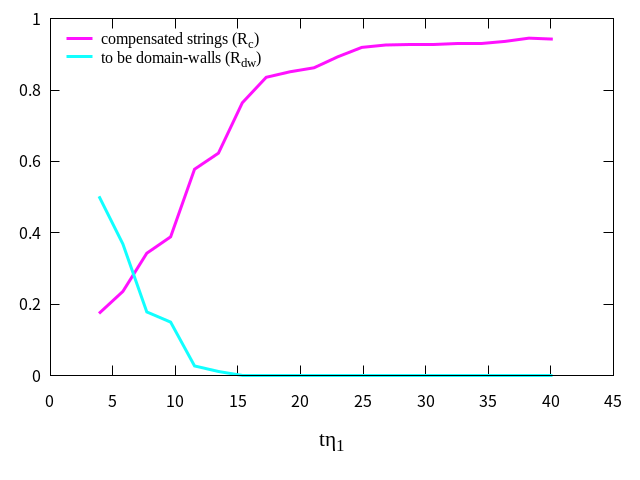
—— $(q_{1},q_{2})=(1,2)$ ——

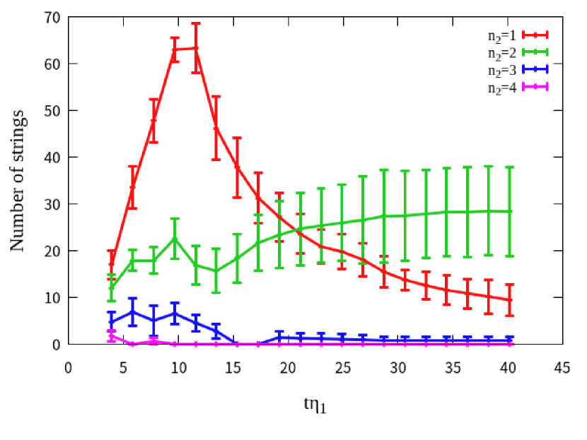
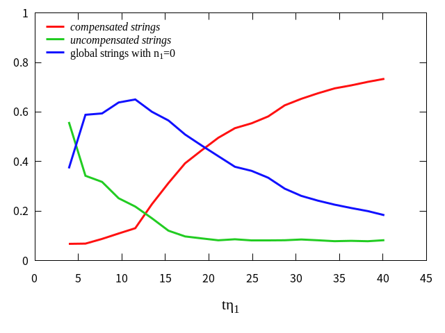
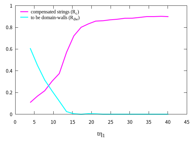
—— $(q_{1},q_{2})=(4,1)$ ——

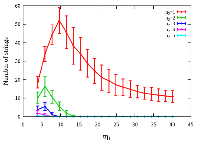
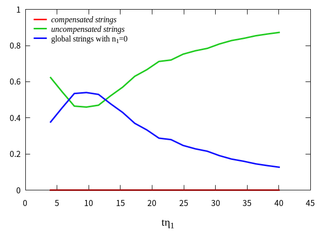
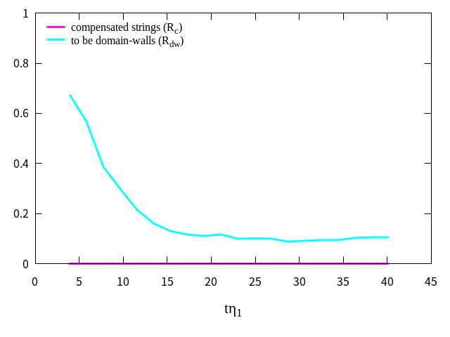
Figure 7: The same figures with Fig. 5 but for $(q_{1},q_{2})=(1,1),(1,2)$ and $(4,1)$.

III.4 Parameter Dependence

So far, we have fixed the model parameters to the values in Eq. (48). Here, we briefly discuss parameter dependencies of the behavior of the string network.

To see the dependence on the charge ratio, we have performed numerical simulations for $(q_{1},q_{2})=(1,1)$ and $(1,2)$, while the other parameters are fixed. In these cases, we have confirmed that the string networks show similar behavior to the case of $(q_{1},q_{2})=(1,4)$, and the number ratio of the compensated strings increases in time as shown in Fig. 7. In fact, the compensated strings are dominated in the late time and thus most of strings take $n_{2}=q_{2}$.

We have also performed numerical simulations for $(q_{1},q_{2})=(4,1)$ with the other parameters fixed. In this case, we found that the string configurations have either $(n_{1},n_{2})=(1,0)$ or $(n_{1},n_{2})=(0,1)$ even at late times, and they do not combine into the compensated strings unlike the case of $(q_{1},q_{2})=(1,4)$ as shown in the bottom panels of Fig. 7. This can be understood by the fact that the long-range force between the uncompensated and the global strings are proportional to the covariant derivative of $\phi_{2}$ around the uncompensated strings (see Sec. IV). In fact, ${\mathscr{D}}_{\theta}\phi_{2}$ around the string configurations of $(n_{1},n_{2})=(1,0)$ is smaller for $(q_{1},q_{2})=(4,1)$ than that for $(q_{1},q_{2})=(1,4)$. As a result, we find that the string network consists of the strings with $(n_{1},n_{2})=(1,0)$ and $(n_{1},n_{2})=(0,1)$ for $(q_{1},q_{2})=(4,1)$ even at a later time.

Altogether, our lattice simulations in the $2+1$ dimensional spacetime suggest that the string network is dominated by the compensated strings $R_{c}\lesssim 1$ for $q_{1}<q_{2}$ and $\eta_{1}>\eta_{2}$, while it is dominated by the uncompensated one for $q_{1}>q_{2}$ and $\eta_{1}>\eta_{2}$. We also find that $R_{\rm dw}\to 0$ for $q_{1}<q_{2}$ and $\eta_{1}>\eta_{2}$, We will discuss the behavior of the string network in the $3+1$ dimensional spacetime in a separate paper, where the $R_{c}$ and $R_{\rm dw}$ can be drastically different from those in the present simulations, since the reconnection rates of the strings can be drastically different in the $3+1$ dimensional spacetime.

We have also performed the simulation for $\kappa=0.3$. In this case, the mass term of $\phi_{2}$ becomes positive at around $\phi_{1}=0$ which stabilizes the symmetry enhancement point, $\phi_{2}=0$ at the center of string core of $\phi_{1}$. This feature is expected to make the correlation between $\phi_{1}$ and $\phi_{2}$ stronger. We have numerically confirmed that the number of $\phi_{2}$ strings formed around the $\phi_{1}$ string tends to be larger for $\kappa>0$ than the case with $\kappa=0$, although we do not discuss details of those tendencies in this paper (see also Urrestilla and Vilenkin (2008)).

IV Interaction between Strings

In this section, we discuss a long-range force between a compensated/uncompensated string with $(n_{1},n_{2})=(n_{1}\neq 0,n_{2A})$ and a global string with $(n_{1},n_{2})=(0,n_{2B})$. We call the former to be the string A and the latter to be the string B. As our simulation was performed in $2+1$ dimensional spacetime, we also consider the string configurations in the $2$-dimensional space. In the $2$-dimensional space, the spatial coordinates of the centers of the string A and B are given by ${\mathbf{r}_{A}}$ and $\mathbf{r}_{B}$, respectively.

In our discussion, we assume $\eta_{1}\gg\eta_{2}$. In this limit, the configurations of $\phi_{1}$ and the gauge field are hardly affected by the configuration of $\phi_{2}$, and hence, we can treat them as the fixed background fields. Besides, we may neglect the $\phi_{2}$ contribution to the Euler-Lagrange equation of the gauge field in Eq. (31) as $c_{1}(\simeq 1)\gg c_{2}$. With such a gauge field configuration, $\mathscr{D}_{\theta}\phi_{1}$ vanishes at the large distance from the string A as in the case of the ANO string.

When the string A and B are well separated, the configuration of $\phi_{2}$ can be approximated by,

$$\phi_{2AB}(\mathbf{r})\equiv\phi_{2}(\mathbf{r};\mathbf{r}_{A},\mathbf{r}_{B})=\frac{\phi_{2A}(\mathbf{r}-\mathbf{r}_{A})\phi_{2B}(\mathbf{r}-\mathbf{r}_{B})}{\eta_{2}}\ ,$$ (51)

where $\phi_{2A}$ and $\phi_{2B}$ are the isolated string configurations of the string A and B. The long-range force between the string A and B can be read off from the difference of the string energy per unit length Bettencourt and Rivers (1995),

$${\mit{\Delta}}E(|\mathbf{r}_{A}-\mathbf{r}_{B}|)=E(\{\phi_{2AB}\})-E(\{\phi_{2A}\})-E(\{\phi_{2B}\})\ .$$ (52)

where the energy functional is given by

$$E(\{\phi_{2}\})=\int d^{2}\mathbf{r}\left[\left|\partial_{r}\phi_{2}\right|^{2}+\frac{1}{r^{2}}\left|{\partial_{\theta}}\phi_{2}-ieq_{2}{A_{\theta}}\phi_{2}\right|^{2}+\frac{\lambda_{2}}{4}\left(|\phi_{2}|^{2}-\eta^{2}_{2}\right)^{2}\right]\ .$$ (53)

In this expression, we have taken ${\mathbf{r}}_{A}=0$, and $(r,\theta)$ are the radius and the azimuthal angle around the string A. In this coordinate system, $A_{\theta}$ is the gauge field configuration around the string.

When the string A and B are well separated, ${\mit{\Delta}E}$ is approximately given by

$${\mit{\Delta}}E\simeq\int d^{2}{\mathbf{r}}\frac{1}{\eta^{2}_{2}}\left(\phi_{2A}\phi^{*}_{2B}\partial_{r}\phi^{*}_{2A}\partial_{r}\phi_{2B}+\frac{1}{r^{2}}\phi_{2A}\phi^{*}_{2B}\mathscr{D}_{\theta}\phi^{*}_{2A}\partial_{\theta}\phi_{2B}+h.c.\right)\ .$$ (54)

Besides, by remembering that

$$|\phi_{2A}|,|\phi_{2B}|\to\eta_{2}+\order{r^{-2}}\ ,$$ (55)

at the large distance, the contributions from the first term in Eq. (54) is subdominant compared to those of the second term. As a result, we find

$${\mit{\Delta}}E \simeq\int d^{2}{\mathbf{r}}\frac{1}{\eta^{2}_{2}}\left(\frac{1}{r^{2}}\phi_{2A}\phi^{*}_{2B}\mathscr{D}_{\theta}\phi^{*}_{2A}\partial_{\theta}\phi_{2B}+h.c.\right)\ ,$$ (56)

$$\simeq 2\,n_{2B}\left(n_{2A}-n_{1}\frac{q_{2}}{q_{1}}\right)\eta^{2}_{2}\int d^{2}{\mathbf{r}}\frac{1}{r^{2}}\frac{\partial\theta_{B}}{\partial\theta}\ .$$ (57)

Here, $\theta_{B}$ is the azimuth angle around the string B, and its derivative with respect to $\theta$ is given by

$$\frac{\partial\theta_{B}}{\partial\theta}=\frac{r(r-|{\mathbf{r}_{A}-\mathbf{r}_{B}}|\cos\theta)}{|\mathbf{r}-\mathbf{r}_{B}|^{2}}\ .$$ (58)

Therefore, the energy difference is given

$${\mit{\Delta}}E(|\mathbf{r}_{A}-\mathbf{r}_{B}|)\simeq n_{2B}\left(n_{2A}-n_{1}\frac{q_{2}}{q_{1}}\right)\eta^{2}_{2}F(|\mathbf{r}_{A}-\mathbf{r}_{B}|),$$ (59)

where $F(x)$ is a decreasing function of $x$.

The long-range force between the uncompensated and the global strings is given by the derivative of ${\mit{\Delta}}E$ with respect to $|\mathbf{r}_{A}-\mathbf{r}_{B}|$. Thus, we find the long-range force is attractive for

$$n_{2B}\left(n_{2A}-n_{1}\frac{q_{2}}{q_{1}}\right)<0\ ,$$ (60)

while it is repulsive for

$$n_{2B}\left(n_{2A}-n_{1}\frac{q_{2}}{q_{1}}\right)>0\ .$$ (61)

With this force, the uncompensated string with $n_{1}=1$ and $n_{2}<4$ and the global string with $n_{1}=0$ and $n_{2}=1$ combine together rather quickly for $(q_{1},q_{2})=(1,4)$. The expression in Eq. (59) also explains the weakness of the attractive force between the string with $(n_{1},n_{2})=(1,0)$ and $(n_{1},n_{2})=(0,1)$ for $(q_{1},q_{2})=(4,1)$.

V Conclusions and Discussions

In this paper, we studied the formation and the evolution of the string network in the Abelian Higgs model with two complex scalar fields. As a special feature of the model, the model possesses a global $U(1)$ symmetry in addition to the $U(1)$ gauge symmetry. Both symmetries are spontaneously broken by the VEVs of the two complex scalar fields.

In this model, the dynamics of the string network is quite rich compared with that in the ordinary Abelian Higgs model with a single complex scalar field. In particular, we found the existence of a new type of string solutions, the uncompensated strings, in addition to the ANO local string. The isolated uncompensated string has a logarithmic divergent energy per unit length as in the case of the global strings, although it is accompanied by non-trivial gauge field configuration.

We also performed the classical lattice simulations in the $2+1$ dimensional spacetime, which confirmed the formation of the uncompensated strings at the phase transition. We also found that most of the uncompensated strings evolve into the compensated strings at later time when the gauge charge of the scalar field with the smaller VEV is larger than that of the scalar field with a larger VEV. Such a behavior can be understood by long range forces between the uncompensated string and the global string.

Finally, we comment on the implications of the results in the present paper to the axion models where $U(1)_{global}$ is identified with the Peccei-Quinn symmetry. As we have mentioned in subsection III.3, we found that all the strings in our simulation for $(q_{1},q_{2})=(1,4)$ have the effective winding number either of $0$ or $\pm 1$ in the direction of the gauge-invariant Goldstone boson at late time. When we apply this model to the axion model, at most one domain wall is attached to the cosmic string below the QCD scale Kawasaki and Nakayama (2013)). Such string-wall network does not cause the infamous domain wall problem. Thus, the axion model with $q_{1}=1$ and $q_{2}\geq 4$ and $\eta_{1}\gg\eta_{2}$ might be free from the domain wall problem even when the $U(1)_{local}$ and $U(1)_{global}$ takes place after inflation. The result of the present paper is, however, based on the simulation in the $2+1$ dimensional spacetime, and hence, not conclusive. We will perform the classical lattice simulation in the $3+1$ dimensional spacetime in a separate paper.

Appendix A Domain Wall Problems in QCD Axion Models

Here, we briefly summarize the axion domain wall problem when we apply the accidental global symmetry, $U(1)_{global}$, to the Peccei-Quinn symmetry Peccei and Quinn (1977a, b); Weinberg (1978); Wilczek (1978) (see also Fukuda et al. (2017, 2018); Ibe et al. (2018)). The Peccei-Quinn mechanism is one of the most successful solutions of the Strong CP problem, where the effective $\theta$-angle of QCD is canceled by the VEV of the pseudo-Nambu-Goldstone boson, the axion (Kawasaki and Nakayama (2013) for review).

To see how the axion appears in the present setup, let us consider the KSVZ axion model Kim (1979); Shifman et al. (1980) and introduce $N_{1}$ and $N_{2}$ of the vector-like multiplets of the fundamental representation of the $SU(3)_{c}$ gauge group of QCD which couple to $\phi_{1}$ and $\phi_{2}^{*}$ through,

$${\cal L}=\phi_{1}\bar{Q}_{1}{Q}_{1}+\phi_{2}^{*}\bar{Q}_{2}{Q}_{2}+h.c.$$ (62)

Here, $(Q_{i},\bar{Q}_{i})$ collectively represents the $N_{i}$ vector-like multiplets ($i=1,2$). We suppress the Yukawa coupling constants for notational simplicity.

Below the $U(1)_{local}$ and $U(1)_{global}$ breaking scales, the vector-multiplets become massive. Then, by integrating out the vector-like multiplets, the couplings of the Goldstone bosons in Eq. (18) to QCD is given by,

$${\cal L}=\frac{g_{s}^{2}}{32\pi^{2}}\left[\left(\frac{N_{1}q_{2}f_{2}^{2}+N_{2}q_{1}f_{1}^{2}}{q_{1}^{2}f_{1}^{2}+q_{2}^{2}f_{2}^{2}}\right)\frac{a}{F_{a}}+\left(N_{1}q_{1}-N_{2}q_{2}\right)\frac{b}{\sqrt{q_{1}^{2}f_{1}^{2}+q_{2}^{2}f_{2}^{2}}}\right]G\tilde{G}\ .$$ (63)

Here, $g_{s}$ is the QCD coupling constant, $G$ and $\tilde{G}$ are the gauge field strength of QCD and its dual. We suppress the color and the Lorentz indices. To satisfy the anomaly free condition of the $U(1)_{local}$ gauge symmetry, we require,

$$N_{1}q_{1}-N_{2}q_{2}=0\ ,$$ (64)

and hence, the effective Goldstone-QCD interactions are reduced to

$${\cal L}=\frac{g_{s}^{2}}{32\pi^{2}}\left[\frac{N_{m}a}{F_{a}}\right]G\tilde{G}\ .$$ (65)

Here, we have introduced a parameter $N_{m}$ by $N_{m}=N_{1}/q_{2}=N_{2}/q_{1}$ ($N_{m}\in\mathbb{Z}^{>0}$). Therefore, the gauge-invariant Goldstone can be identified with the QCD axion.

Now, let us discuss how the axion evolves in the cosmological history. Let us assume that the $U(1)$ symmetry breaking takes place after inflation. Then, the axion locally settles down to a point at the bottom of the scalar potential in Eq. (6) after the phase transition. The axion, however, winds around the cosmic string with an effective winding number,

$$n_{\rm eff}=n_{1}q_{2}-n_{2}q_{1}\ ,$$ (66)

in the domain of the axion $[0,2\pi F_{a})$ as given in Eq. (20). Below the QCD scale, the axion coupling to QCD in Eq. (65) results in a periodic axion potential with a period, $F_{a}/N_{m}$. Therefore, the axion potential gives rise the energy contrasts around the cosmic strings and the cosmic strings are attached by $N_{\rm dw}=N_{m}\times|n_{\rm eff}|$ domain walls. For $|N_{\rm dw}|>1$, the string-wall network is stable and immediately dominates the energy density of the universe, which conflicts with the Standard Cosmology..

Around the compensated strings, i.e. $n_{\rm eff}=0$, on the other hand, no walls are formed, and hence, it does not cause cosmological problems. Besides, the string-wall network with $N_{\rm dw}=1$ also does not cause cosmological problems, since the network is not stable and decays immediately after the QCD phase transition Vilenkin and Everett (1982); Hiramatsu et al. (2012). The latter possibility requires $N_{m}=1$ and $|n_{\rm eff}|=1$. Therefore, the domain wall problems in the axion model can be avoided if the cosmic strings evolves into either $R_{\rm c}\to 1$ or $R_{\rm dw}\to 0$ at a later time.

References

- Nielsen and Olesen (1973) H. B. Nielsen and P. Olesen, Nucl. Phys. B61, 45 (1973), [,302(1973)].
- Vilenkin and Shellard (2000) A. Vilenkin and E. P. S. Shellard, Cosmic Strings and Other Topological Defects (Cambridge University Press, 2000).
- Albrecht and Turok (1985) A. Albrecht and N. Turok, Phys. Rev. Lett. 54, 1868 (1985).
- Albrecht and Turok (1989) A. Albrecht and N. Turok, Phys. Rev. D40, 973 (1989).
- Bennett and Bouchet (1990) D. P. Bennett and F. R. Bouchet, Phys. Rev. D41, 2408 (1990).
- Allen and Shellard (1990) B. Allen and E. P. S. Shellard, Phys. Rev. Lett. 64, 119 (1990).
- Vincent et al. (1997) G. R. Vincent, M. Hindmarsh, and M. Sakellariadou, Phys. Rev. D56, 637 (1997), arXiv:astro-ph/9612135 [astro-ph] .
- Martins and Shellard (2006) C. J. A. P. Martins and E. P. S. Shellard, Phys. Rev. D73, 043515 (2006), arXiv:astro-ph/0511792 [astro-ph] .
- Ringeval et al. (2007) C. Ringeval, M. Sakellariadou, and F. Bouchet, JCAP 0702, 023 (2007), arXiv:astro-ph/0511646 [astro-ph] .
- Olum and Vanchurin (2007) K. D. Olum and V. Vanchurin, Phys. Rev. D75, 063521 (2007), arXiv:astro-ph/0610419 [astro-ph] .
- Fraisse et al. (2008) A. A. Fraisse, C. Ringeval, D. N. Spergel, and F. R. Bouchet, Phys. Rev. D78, 043535 (2008), arXiv:0708.1162 [astro-ph] .
- Blanco-Pillado et al. (2011) J. J. Blanco-Pillado, K. D. Olum, and B. Shlaer, Phys. Rev. D83, 083514 (2011), arXiv:1101.5173 [astro-ph.CO] .
- Vincent et al. (1998) G. Vincent, N. D. Antunes, and M. Hindmarsh, Phys. Rev. Lett. 80, 2277 (1998), arXiv:hep-ph/9708427 [hep-ph] .
- Moore et al. (2002) J. N. Moore, E. P. S. Shellard, and C. J. A. P. Martins, Phys. Rev. D65, 023503 (2002), arXiv:hep-ph/0107171 [hep-ph] .
- Bettencourt and Rivers (1995) L. M. A. Bettencourt and R. J. Rivers, Phys. Rev. D51, 1842 (1995), arXiv:hep-ph/9405222 [hep-ph] .
- Bettencourt et al. (1997) L. M. A. Bettencourt, P. Laguna, and R. A. Matzner, Phys. Rev. Lett. 78, 2066 (1997), arXiv:hep-ph/9612350 [hep-ph] .
- Salmi et al. (2008) P. Salmi, A. Achucarro, E. J. Copeland, T. W. B. Kibble, R. de Putter, and D. A. Steer, Phys. Rev. D77, 041701 (2008), arXiv:0712.1204 [hep-th] .
- Achucarro and de Putter (2006) A. Achucarro and R. de Putter, Phys. Rev. D74, 121701 (2006), arXiv:hep-th/0605084 [hep-th] .
- Pen et al. (1997) U.-L. Pen, U. Seljak, and N. Turok, Phys. Rev. Lett. 79, 1611 (1997), arXiv:astro-ph/9704165 [astro-ph] .
- Durrer et al. (1999) R. Durrer, M. Kunz, and A. Melchiorri, Phys. Rev. D59, 123005 (1999), arXiv:astro-ph/9811174 [astro-ph] .
- Yamaguchi et al. (1999) M. Yamaguchi, M. Kawasaki, and J. Yokoyama, Phys. Rev. Lett. 82, 4578 (1999), arXiv:hep-ph/9811311 [hep-ph] .
- Yamaguchi et al. (2000) M. Yamaguchi, J. Yokoyama, and M. Kawasaki, Phys. Rev. D61, 061301 (2000), arXiv:hep-ph/9910352 [hep-ph] .
- Yamaguchi (1999) M. Yamaguchi, Phys. Rev. D60, 103511 (1999), arXiv:hep-ph/9907506 [hep-ph] .
- Yamaguchi and Yokoyama (2002) M. Yamaguchi and J. Yokoyama, Phys. Rev. D66, 121303 (2002), arXiv:hep-ph/0205308 [hep-ph] .
- Yamaguchi and Yokoyama (2003) M. Yamaguchi and J. Yokoyama, Phys. Rev. D67, 103514 (2003), arXiv:hep-ph/0210343 [hep-ph] .
- Cui et al. (2008) Y. Cui, S. P. Martin, D. E. Morrissey, and J. D. Wells, Phys. Rev. D77, 043528 (2008), arXiv:0709.0950 [hep-ph] .
- Hiramatsu et al. (2013) T. Hiramatsu, Y. Sendouda, K. Takahashi, D. Yamauchi, and C.-M. Yoo, Phys. Rev. D88, 085021 (2013), arXiv:1307.0308 [astro-ph.CO] .
- Hindmarsh et al. (2019) M. Hindmarsh, J. Lizarraga, J. Urrestilla, D. Daverio, and M. Kunz, Phys. Rev. D99, 083522 (2019), arXiv:1812.08649 [astro-ph.CO] .
- Peccei and Quinn (1977a) R. D. Peccei and H. R. Quinn, Phys. Rev. Lett. 38, 1440 (1977a).
- Peccei and Quinn (1977b) R. D. Peccei and H. R. Quinn, Phys. Rev. D16, 1791 (1977b).
- Weinberg (1978) S. Weinberg, Phys. Rev. Lett. 40, 223 (1978).
- Wilczek (1978) F. Wilczek, Phys. Rev. Lett. 40, 279 (1978).
- Lazarides and Shafi (1982) G. Lazarides and Q. Shafi, Phys. Lett. B115, 21 (1982).
- Barr et al. (1982) S. M. Barr, X. C. Gao, and D. Reiss, Phys. Rev. D26, 2176 (1982).
- Choi and Kim (1985) K. Choi and J. E. Kim, Phys. Rev. Lett. 55, 2637 (1985).
- Fukuda et al. (2017) H. Fukuda, M. Ibe, M. Suzuki, and T. T. Yanagida, Phys. Lett. B771, 327 (2017), arXiv:1703.01112 [hep-ph] .
- Fukuda et al. (2018) H. Fukuda, M. Ibe, M. Suzuki, and T. T. Yanagida, JHEP 07, 128 (2018), arXiv:1803.00759 [hep-ph] .
- Ibe et al. (2018) M. Ibe, M. Suzuki, and T. T. Yanagida, JHEP 08, 049 (2018), arXiv:1805.10029 [hep-ph] .
- Hawking (1987) S. W. Hawking, Moscow Quantum Grav.1987:0125, Phys. Lett. B195, 337 (1987).
- Lavrelashvili et al. (1987) G. V. Lavrelashvili, V. A. Rubakov, and P. G. Tinyakov, JETP Lett. 46, 167 (1987), [Pisma Zh. Eksp. Teor. Fiz.46,134(1987)].
- Giddings and Strominger (1988) S. B. Giddings and A. Strominger, Nucl. Phys. B307, 854 (1988).
- Coleman (1988) S. R. Coleman, Nucl. Phys. B310, 643 (1988).
- Gilbert (1989) G. Gilbert, Nucl. Phys. B328, 159 (1989).
- Banks and Seiberg (2011) T. Banks and N. Seiberg, Phys. Rev. D83, 084019 (2011), arXiv:1011.5120 [hep-th] .
- Lee et al. (2006) P. A. Lee, N. Nagaosa, and X.-G. Wen, Rev. Mod. Phys. 78, 17 (2006).
- Chernodub et al. (2006a) M. N. Chernodub, A. Schiller, and E. M. Ilgenfritz, PoS LAT2005, 295 (2006a), arXiv:hep-lat/0509088 [hep-lat] .
- Chernodub et al. (2006b) M. N. Chernodub, E. M. Ilgenfritz, and A. Schiller, Phys. Rev. B73, 100506 (2006b), arXiv:cond-mat/0512111 [cond-mat] .
- Bock et al. (2007) M. Bock, M. N. Chernodub, E. M. Ilgenfritz, and A. Schiller, Phys. Rev. B76, 184502 (2007), arXiv:0705.1528 [cond-mat.str-el] .
- Babaev et al. (2009) E. Babaev, J. Jäykkä, and M. Speight, Phys. Rev. Lett 103, 237002 (2009), arXiv:0903.3339 [cone-mat.supr-com] .
- Catelani and Yuzbashyan (2010) G. Catelani and E. A. Yuzbashyan, Phys. Rev. A 81, 033629 (2010).
- Forgȧcs and Lukȧcs (2017) P. Forgȧcs and Á. Lukȧcs, Phys. Rev. D95, 035003 (2017), arXiv:1612.03151 [hep-th] .
- Forgȧcs and Lukȧcs (2016) P. Forgȧcs and Ȧ. Lukȧcs, Phys. Rev. D94, 125018 (2016), arXiv:1608.00021 [hep-th] .
- Saffin (2005) P. M. Saffin, JHEP 09, 011 (2005), arXiv:hep-th/0506138 [hep-th] .
- Urrestilla and Vilenkin (2008) J. Urrestilla and A. Vilenkin, JHEP 02, 037 (2008), arXiv:0712.1146 [hep-th] .
- Kawasaki and Nakayama (2013) M. Kawasaki and K. Nakayama, Ann. Rev. Nucl. Part. Sci. 63, 69 (2013), arXiv:1301.1123 [hep-ph] .
- Kim (1979) J. E. Kim, Phys. Rev. Lett. 43, 103 (1979).
- Shifman et al. (1980) M. A. Shifman, A. I. Vainshtein, and V. I. Zakharov, Nucl. Phys. B166, 493 (1980).
- Vilenkin and Everett (1982) A. Vilenkin and A. E. Everett, Phys. Rev. Lett. 48, 1867 (1982).
- Hiramatsu et al. (2012) T. Hiramatsu, M. Kawasaki, K. Saikawa, and T. Sekiguchi, Phys. Rev. D85, 105020 (2012), [Erratum: Phys. Rev.D86,089902(2012)], arXiv:1202.5851 [hep-ph] .