Jamming and replica symmetry breaking of weakly disordered crystals

Abstract

We discuss the physics of crystals with small polydispersity near the jamming transition point. For this purpose, we introduce an effective single-particle model taking into account the nearest neighbor structure of crystals. The model can be solved analytically by using the replica method in the limit of large dimensions. In the absence of polydispersity, the replica symmetric solution is stable until the jamming transition point, which leads to the standard scaling of perfect crystals. On the contrary, for finite polydispersity, the model undergoes the full replica symmetry breaking (RSB) transition before the jamming transition point. In the RSB phase, the model exhibits the same scaling as amorphous solids near the jamming transition point. These results are fully consistent with the recent numerical simulations of crystals with polydispersity. The simplicity of the model also allows us to derive the scaling behavior of the vibrational density of states that can be tested in future experiments and numerical simulations.

I Introduction

Physics of crystal and amorphous solids are qualitatively different. For instance, low frequency eigenmodes of crystals are phonon, and thus the vibrational density of states $D(\omega)$ follows the Debye law $D(\omega)\sim\omega^{d-1}$ where $d$ denotes the spatial dimensions Kittel et al. (1976). On the contrary, amorphous solids have excess non-phonon excitations. As a consequence, the density of states normalized by the Debye’s prediction $D(\omega)/\omega^{d-1}$ shows a peak at a certain frequency $\omega=\omega_{\rm BP}$ Buchenau et al. (1984); Malinovsky and Sokolov (1986); Grigera et al. (2003); Shintani and Tanaka (2008); Kaya et al. (2010). This phenomenon is known as the boson peak and thought to be one of the universal properties of amorphous solids Phillips and Anderson (1981).

Crystal and amorphous solids also show distinct elastic properties near the (un) jamming transition point at which constituent particles lose contact, and simultaneously the pressure vanishes van Hecke (2009). Here we focus on the jamming of spherical and frictionless particles interacting with finite and repulsive potentials. The scaling of these models is now well understood due to extensive numerical simulations O’Hern et al. (2003); van Hecke (2009) and theories Wyart et al. (2005); Wyart (2005); Charbonneau et al. (2014, 2017). The shear modulus $G$ of crystals does not show the strong pressure $p$ dependence and remains a constant at the jamming transition point Goodrich et al. (2014); Tong et al. (2015). On the contrary, $G$ of amorphous solids shows the power law behavior $G\sim p^{1/2}$ and vanishes at the jamming transition point O’Hern et al. (2003); van Hecke (2009). The behavior of $G$ is directly related to the contact number per particle $Z$ as $G\propto\delta Z\equiv Z-Z_{\rm iso}$ Wyart (2005). Here $Z_{\rm iso}$ denotes the contact number when a system is isostatic, i.e., the number of constraints is the same as the number of degrees of freedom Maxwell (1864); Alexander (1998). At the jamming transition point, $\delta Z>0$ for perfect crystals, leading to $G>0$, whereas $\delta Z=0$ for amorphous solids, leading to $G=0$ van Hecke (2009); O’Hern et al. (2003).

Crystal and amorphous are two extreme states of solids: the former is a state free from disorder while the latter is a state of maximum disorder. From both theoretical and practical points of views, it is important to understand how the physical properties shift from that of crystal to amorphous on the increase of the strength of disorder. Previous numerical simulations show that small disorder only play a moderate role far from the jamming transition point ($p\sim 1$). For instance, numerical studies of crystals with polydispersity show that the amplitude of the boson peak $D(\omega_{\rm BP})/\omega_{\rm BP}^{d-1}$ only continuously increases on the increase of the polydispersity $\eta$, if $\eta$ is small enough Mizuno et al. (2013); Guo-Hua et al. (2014). Near the jamming transition point $p\ll 1$, on the contrary, even small disorder dramatically change the physical properties of crystals. More and more non-phonon modes appear as $p$ decreases, eventually leading to the divergence of $D(\omega_{\rm BP})/\omega_{\rm BP}^{d-1}$ in the jamming limit $p\to 0$, in sharp contrast to perfect crystals where $D(\omega)$ does not show the strong $p$ dependence. Furthermore, for crystals with small defects or polydispersity, $G$ and $\delta Z$ exhibit the same power laws of amorphous solids sufficiently near the jamming transition point Goodrich et al. (2014); Tong et al. (2015). In particular, $G$ and $\delta Z$ vanish at the jamming transition point if there is even infinitesimally small polydispersity Mari et al. (2009); Tong et al. (2015), while for perfect crystals, $G$ and $\delta Z$ remain finite.

Our aim here is to construct a solvable mean field model being able to describe the above striking effects of disorder on crystals near the jamming transition point. We consider a model in the limit of large dimensions, which is a popular mean field limit in theoretical physics Georges et al. (1996); Parisi and Zamponi (2010). In this limit, only the first virial corrections give a relevant contribution Frisch and Percus (1999); Parisi and Zamponi (2010). For short-range potential such as hard spheres, this implies that the information of nearest neighbor structures is enough to describe the physics. Motivated by this consideration, we introduce an effective single-particle model that only takes into account the interactions between a particle of interest and nearest-neighbor particles. For zero polydispersity $\eta=0$, our model correctly reproduces the scaling of perfect crystals. For finite $\eta$, on the contrary, our model predicts that the existence of the replica symmetry breaking (RSB) transition Mézard et al. (1987) at finite pressure $p=p_{\rm RSB}$. For $p\leq p_{\rm RSB}$, the model exhibits the same scaling as amorphous solids. Thereby, our model can reproduce the sharp cross-over from the scaling of crystal to amorphous observed in previous numerical simulations of weakly disordered crystals.

II Model

Figure 1: Jaming configurations for $d=2$ and $\eta=0$. The gray disk denotes the tracer particle, and the black disks denote nearest neighbors. The blue solid line denotes the equidistant line from the tracer particle, and the red dashed lines denote contacts. (a) Configuration of the hexagonal close-packing. The nearest neighbors are arranged periodically on the equidistant line. (b) Configuration of our model. The nearest neighbors are placed randomly on the equidistant line.

We consider a tracer particle surrounded by $M$ frozen nearest-neighbor (NN) particles in the limit of the large spatial dimensions. In $d$ spatial dimensions, the tracer particle has $d$ degrees of freedom, implying that the model becomes isostatic when the contact number is $Z=Z_{\rm iso}=d$ . The tracer and NN particles interact with the one-sided harmonic potential:

$$V(\bm{X})=\sum_{\mu=1}^{M}v(h^{\mu}),\ h^{\mu} =\sqrt{d}\left(\left|\bm{X}-\bm{y}^{\mu}\right|-\sigma^{\mu}\right),$$ (1)

where $v(x)=x^{2}\theta(-x)/2$, and the pre-factor $\sqrt{d}$ of the gap function $h^{\mu}$ is necessary to keep $h^{\mu}=O(1)$ in the $d\to\infty$ limit, see Appendix A for details. $\bm{X}=\{X_{1},\cdots,X_{d}\}$ and $\bm{y}^{\mu}=\{y_{1}^{\mu},\cdots,y_{d}^{\mu}\}$ denote the positions of the tracer and $\mu$-th NN particle, respectively. $\sigma^{\mu}$ denotes the interaction range between the tracer and $\mu$-th NN particle. We assume that $\sigma^{\mu}$ can be written as

$$\sigma^{\mu}=\sigma\left(1+\frac{1}{d}b^{\mu}\right),$$ (2)

where $\sigma$ controls the mean size of particles, and $b^{\mu}$ denotes the polydispersity. The pre-factor of $b^{\mu}$, $1/d$, is necessary to keep the relative interaction volume remains finite in the large dimensional limit: $\lim_{d\to\infty}(\sigma^{\mu}/\sigma^{\nu})^{d}=e^{b^{\mu}-b^{\nu}}$. $b^{\mu}$ follows the normal distribution of zero mean and variance $\eta^{2}$:

$$P(b^{\mu})=\frac{1}{\sqrt{2\pi\eta^{2}}}\exp\left[-\frac{(b^{\mu})^{2}}{2\eta^{2}}\right].$$ (3)

The NN particles are homogeneously distributed on the surface of the hypersphere of the radius $\sqrt{d}$, namely, the distribution function of $\bm{y}^{\mu}$ is given by

$$P(\bm{y}^{\mu})=\frac{\delta(\bm{y}^{\mu}\cdot\bm{y}^{\mu}-d)}{\int d\bm{y}^{\mu}\delta(\bm{y}^{\mu}\cdot\bm{y}^{\mu}-d)}.$$ (4)

To get the physical intuition about the model, we first explain the behavior at the jamming transition point in $d=2$ in the absence of the polydispersity $\eta=0$, comparing it with the hexagonal packing. For the the hexagonal packing, the NN particles are arranged periodically on the equidistant line from the tracer particle (Fig. 1(a)). On the contrary, for our model at the jamming transition point, the NN particles are randomly distributed on the equidistant line (Fig. 1(b)). The tracer is in contact with all NN particles, as in the case of hexagonal packing, leading to a hyperstatic configuration when the number of the NN particles $M$ is larger than $Z_{\rm iso}$.

The same story holds in general $d$ as long as $\eta=0$: the jamming occurs when $\sigma\equiv\sigma_{J}^{0}=\sqrt{d}$, at which $\bm{X}=0$ and $h^{\mu}=0$ for all $\mu$, meaning that the tracer particle is in contact with all NN particles, leading to a hyperstatic configuration when $M>Z_{\rm iso}$. On the contrary, for $\eta>0$, the jamming configuration is non-trivial, which we shall discuss in this manuscript.

III Marginal stability

The previous works for the mean field models of the jamming transition unveiled that the systems undergo replica symmetry breaking (RSB) before reaching the jamming transition point. In the RSB phase the systems are marginally stable Mézard et al. (1987); Franz et al. (2015). Here we show that the contact number in the RSB phase can be calculated by using the marginal stability.

At zero temperature, the stability of the system can be discussed by observing the Hessian of the interaction potential:

$$\mathcal{H}_{ij} =\frac{1}{d}\frac{\partial V(\bm{X})}{\partial X_{i}\partial X_{j}}\sim\frac{1}{d}\sum_{\mu=1}^{M}\left(y_{i}^{\mu}y_{j}^{\mu}+\delta_{ij}h_{\mu}\right)\theta(-h_{\mu}),$$ (5)

where the $1/d$ prefactor is necessary to make $H_{ij}=O(1)$, and we only keep the relevant terms in the limit of $d\to\infty$. In this limit, $y_{i}^{\mu}$ can be identified with the i.i.d. Gaussian random variable of zero mean and unit variance, see Appendix B. Thus, $\mathcal{H}_{ij}$ can be considered as a Wishart matrix Livan et al. (2018) with an additional diagonal term. The eigenvalue distribution of $\mathcal{H}_{ij}$ follows the Marchenko-Pastur distribution Franz et al. (2017):

$$\rho(\lambda)=\frac{1}{2\pi}\frac{\sqrt{(\lambda-\lambda_{-})(\lambda_{+}-\lambda)}}{\lambda+p},\ \lambda_{\pm}=\left(\sqrt{z}\pm 1\right)^{2}-p,$$ (6)

where we have defined the contact number per degree of freedom $z=Z/d$ and pressure $p$ as

$$z=\frac{1}{d}\sum_{\mu=1}^{M}\theta(-h^{\mu}),\ p=-\frac{1}{d}\sum_{\mu=1}^{M}\theta(-h^{\mu})h^{\mu}.$$ (7)

In the RSB phase, the marginal stability requires $\lambda_{-}=0$ Mézard et al. (1987); Franz et al. (2015). This condition with Eq. (6) determines $z$ as a function of $p$:

$$z=(1+p^{1/2})^{2}.$$ (8)

This result implies that (i) the model is isostatic $z=z_{\rm iso}=1$ at the jamming transition point $p=0$ , and (ii) $z$ exhibits the square root scaling $\delta z=z-z_{\rm iso}\propto p^{1/2}$ for $p\ll 1$. Those properties are the same as amorphous solids consisting of soft harmonic particles O’Hern et al. (2003) and a mean-field model of the jamming transition Franz et al. (2017).

Here we used a rather heuristic argument to calculate $z$ in the RSB phase. But the same result can be derived by directly solving the RSB equation, see Appendix E.

IV Replica method

The RSB is a consequence of the complex structure of the free energy landscape of amorphous solids near the jamming transition point Charbonneau et al. (2017). On the contrary, perfect crystals or nearly perfect crystals have a unique minimum, in other words, the systems are in the replica symmetric (RS) phase. Since the RS phase is not marginally stable, we can not use Eq. (7). Instead, we calculate $z$ by using the replica method Mézard et al. (1987). The calculation is very similar to that of the perceptron, which was previously investigated as a mean-field model of the jamming transition Franz and Parisi (2016); Franz et al. (2017). Therefore, below we just briefly sketch how to calculate $z$ as a function of $p$. The details of the calculations are provided in Appendix C.

To calculate $z$ and $p$, it is convenient to introduce the gap distribution:

$$g(h) =\frac{1}{d}\left\langle\sum_{\mu=1}^{M}\delta(h-h^{\mu})\right\rangle=\frac{\delta F}{\delta v(h)},$$ (9)

where $F$ denotes the free energy, and $\langle\bullet\rangle$ denotes the average for both quenched disorder and thermal fluctuation. Using $g(h)$, $z$ and $p$ are calculated as

$$z=\int_{-\infty}^{\infty}dhg(h)\theta(-h),\ p=-\int_{-\infty}^{\infty}dhg(h)\theta(-h)h.$$ (10)

We calculate $F$ by using the replica method:

$$-\beta F=\lim_{d\to\infty}\frac{\left[\log\mathcal{Z}\right]_{b,\bm{y}}}{d}=\lim_{n\to 0,d\to\infty}\frac{\log\left[\mathcal{Z}^{n}\right]_{b,\bm{y}}}{nd},$$ (11)

where $\mathcal{Z}$ denotes the partition function:

$$\mathcal{Z}=\int d\bm{x}e^{-\beta V(\bm{X})}.$$ (12)

$\beta$ represents the inverse temperature. In this work, we investigate the model only in the zero temperature limit $\beta\to\infty$. Investigations at finite $\beta$ are left for future work. The square brackets in Eq. (11) denote the average for the quenched randomnesses:

$$\left[\bullet\right]_{b,\bm{y}}=\prod_{\mu=1}^{M}\int db^{\mu}P(b^{\mu})\int d\bm{y}^{\mu}P(\bm{y}^{\mu})\bullet,$$ (13)

where $P(b^{\mu})$ and $P(\bm{y}^{\mu})$ are given by Eq. (3) and (4), respectively. By using the saddle point method, one can represent $F$ as a function of the correlation among the replicas (see Appendix B for details):

$$Q_{ab}=\left\langle\bm{X}^{a}\cdot\bm{X}^{b}\right\rangle,\ a,b=1,\cdots,n,$$ (14)

where $\bm{X}^{a}$ and $\bm{X}^{b}$ denote the positions of the $a$-th and $b$-th replicas, respectively. As the free energy has a single minimum in the RS phase, there is no reason to distinguish a specific pair of replicas $ab$, implying that $Q_{ab}$ is written as

$$Q_{ab}=\begin{cases}q_{0}&(a=b),\\ q&(a\neq b).\end{cases}$$ (15)

We can calculate $q$ and $q_{0}$ by solving the saddle point equations: $\partial_{q_{0}}F=0$ and $\partial_{q}F=0$ (see Appendix C for details). Substituting back the results to $F$, we obtain the free energy at the saddle point, which allows us to calculate $g(h)$, $z$, and $p$. Below, we will show the results only for $M=10d$, but we confirmed that the qualitatively same results are obtained for different values of $M$.

To see the stability of the RS Ansatz, we calculate the minimal eigenvalue $\lambda_{-}$ by substituting the RS results for $z$ and $p$ into Eq. (6). The RS-RSB transition point is determined by the condition $\lambda_{-}=0$.

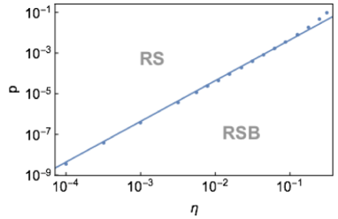
Figure 2: Phase diagram for $M=10d$. Markers denote the numerical results, while solid line denotes a quadratic fit $p\propto\eta^{2}$.

In Fig. 2, we show the RS-RSB phase diagram in the $\eta-p$ plane. It is noteworthy that the RSB always occurs at a finite pressure $p=p_{\rm RSB}\sim\eta^{2}$ before reaching the jamming transition point $p=0$ whenever $\eta>0$.

V Scaling of contact number

Figure 3: Scaling of the excess contact number $\delta z$ as a function of the pressure $p$ for $M=10d$. (a) Filled circles denote the exact results. $\star$ denotes the RSB transition point. The black solid line denotes $z=M/d$, the blue dotted line denotes $\delta z\sim p$, and the red dashed line denotes $\delta z\sim p^{1/2}$. (b) The same data with the rescaled pressure.

Following the above procedures, we calculate $z$ for several $\eta$. We summarize our results in Fig. 3. There are three different scaling regions. For $p\gg\eta$, $z$ takes a constant value $z\approx M/d$, meaning that the tracer particle contact with most NN particles, see the black line. For $\eta^{2}\ll p\ll\eta$, the contact number decreases as $\delta z\sim p$, see the blue dotted line. At $p=p_{\rm RSB}\sim\eta^{2}$, the RS solution becomes unstable, and for $p\leq p_{\rm RSB}$, one should use the RSB result Eq. (8). For $p\ll\eta^{2}$, Eq. (8) predicts $\delta z\sim p^{1/2}$, see the red dashed line.

For $p\geq p_{\rm RSB}$, the results for different $\eta$ collapse on a single curve if one plots $\delta z$ as a function of $\eta^{-1}p$, see Fig. 3 (b). This scaling is consistent with a previous numerical simulation Tong et al. (2015) and perturbation theory Acharya et al. (2020). Remarkably, the above scaling implies that the two limits $\eta\to 0$ and $p\to 0$ are not commutative: if one takes the limit $\eta\to 0$ first and then takes the limit $p\to 0$, one gets $\delta z>0$, contrary, if one takes the limits in reverse order, one gets $\delta z=0$.

VI Density of states

An important quantity to characterize the physics of solids is the vibrational density of states $D(\omega)$, which is a distribution of the eigen-frequency $\omega=\sqrt{\lambda}$. By using Eq. (6), $D(\omega)$ is calculated as $D(\omega)=2\omega\rho(\omega^{2})$. Near the jamming transition point for small $\omega$, $D(\omega)$ asymptotically behaves as

$$D(\omega)\sim\begin{cases}{\rm constant}&\delta z\ll\omega\ll 1\\ \delta z^{-2}\omega^{2}&\omega_{0}<\omega\ll\delta z\\ 0&\omega\leq\omega_{0},\end{cases}$$ (16)

where $\omega_{0}=\sqrt{\lambda_{-}}$. In the RS phase, $\omega_{0}>0$ and $D(\omega)$ has a finite gap . $\omega_{0}$ decreases on the decreasing of $p$ and eventually vanishes at $p=p_{\rm RSB}$. In the RSB phase $p\leq p_{\rm RSB}$, $\omega_{0}=0$ and $D(\omega)$ is gapless. For $\omega\ll 1$, the density of states exhibits the quadratic scaling $D(\omega)\sim\omega^{2}$. This is the same result as previous mean field theories of amorphous solids DeGiuli et al. (2014); Franz et al. (2015). In the jamming limit $p\to 0$ for $\eta>0$, $D(\omega)$ always exhibits the plateau for small $\omega$, which is fully consistent with previous numerical simulations of weakly disordered crystals near the jamming transition point Goodrich et al. (2014); Charbonneau et al. (2019).

Figure 4: Scaling of the boson peak. (a) and (b) show the $p$ and $\eta$ dependence of the boson peak intensities, respectively.

Now we want to calculate the boson peak. For comparison with numerical simulations, we consider the height of $D(\omega)/\omega^{m}$ at its peak $\omega=\omega_{\rm BP}$, where $m=1$ and $m=2$ correspond to the Debye predictions in two and three spatial dimensions, respectively. Using the scaling of $\delta z$ and (16), one can deduce the asymptotic behavior for $m\leq 2$  as a function of $p$:

$$\frac{D(\omega_{\rm BP})}{\omega_{\rm BP}^{m}}\sim\begin{cases}{\rm constant}&\eta\ll p\ll 1\\ \eta^{m}p^{-m}&\eta^{2}\ll p\ll\eta\\ p^{-\frac{m}{2}}&p\ll\eta^{2},\end{cases}$$ (17)

Eq. (17) suggests that the boson peak intensity diverges in the jamming limit $p\to 0$. This scaling is the same of that of amorphous solids near the jamming transition point observed by a numerical simulation of three dimensional harmonic spheres Mizuno et al. (2017). Repeating the similar calculation, one can derive the scaling of the boson peak intensity as a function of $\eta$:

$$\frac{D(\omega_{\rm BP})}{\omega_{\rm BP}^{m}}\sim\begin{cases}p^{-\frac{m}{2}}&\eta\sim 1\\ \eta^{m}p^{-m}&p\ll\eta\ll p^{1/2}\\ {\rm constant}&\eta\ll p,\end{cases}$$ (18)

Eq. (18) suggests that, on the increase of the polydispersity $\eta$, the boson peak begins to increase at $\eta\sim p$. This is consistent with a previous numerical simulation of crystals with small polydispersity Tong et al. (2015). In Fig. 4, we summarize the scaling of the boson peak intensity predicted by the above equations. It is interesting to test the full scaling behavior by experiments and numerical simulations.

VII Summary and discussion

In this work, we have introduced a mean field model to describe the jamming transition of crystals with small polydispersity. We solved the model by using the replica method and determined the full scaling behaviors of the contact number and density of states above the jamming transition point. The results are well agreed with previous numerical simulations.

Another important quantity to characterize the jamming transition is the gap distribution Charbonneau et al. (2014). In Refs. Charbonneau et al. (2019); Tsekenis (2020), it is shown that the gap distribution of the disordered crystal has a different critical exponent from both perfect crystals and amorphous solids. It is an interesting future work to see if our model can explain this intriguing behavior of the gap distribution.

Appendix A Interaction potential in the large dimensional limit

Our model consists of a tracer particle and $M$ nearest neighbor (NN) particles. The tracer is located in a $d$-dimensional hypersphere, and the $M$ NN particles are fixed on the surface of the hypersphere. The interaction potential is given by

$$V(\bm{X})=\sum_{\mu=1}^{M}v(h^{\mu}),$$ (19)

where $v(h)=h^{2}\theta(-h)/2$ and

$$h^{\mu}=\sqrt{d}\left(\left|\bm{X}-\bm{y}^{\mu}\right|-\sigma^{\mu}\right).$$ (20)

Here the pre-factor $\sqrt{d}$ is necessary to keep $V(\bm{X})=O(d^{0})$ in the $d\to\infty$ limit, as we will see below. $\bm{X}=\{X_{1},\cdots,X_{d}\}$ and $\bm{y}^{\mu}=\{y_{1}^{\mu},\cdots,y_{d}^{\mu}\}$ denote the positions of the tracer and $\mu$-th NN, respectively. The distribution of $\bm{y}^{\mu}$ is

$$P(\bm{y}^{\mu})=\frac{\delta(\bm{y}^{\mu}\cdot\bm{y}^{\mu}-d)}{\int d\bm{y}^{\mu}\delta(\bm{y}^{\mu}\cdot\bm{y}^{\mu}-d)}.$$ (21)

$\sigma^{\mu}$ denotes the interaction range between the tracer and $\mu$-th obstacles. We consider that $\sigma^{\mu}$ has the following form

$$\sigma^{\mu}=\sigma\left(1+\frac{1}{d}b^{\mu}\right),$$ (22)

where $\sigma$ controls the mean size of the particles, and $b^{\mu}$ denotes the polydispersity. $b^{\mu}$ follows the normal distribution of zero mean and variance $\eta^{2}$:

$$P(b^{\mu})=\frac{1}{\sqrt{2\eta^{2}\pi}}\exp\left[-\frac{(b^{\mu})^{2}}{2\eta^{2}}\right].$$ (23)

For $\eta=0$, the jamming transition occurs at $\sigma=\sigma_{J}^{0}\equiv\sqrt{d}$ at which $\bm{X}=0$ and $\tilde{h}^{\mu}=0$ for all $\mu$. We expand $\sigma$ around $\sigma_{J}^{0}$ as

$$\sigma=\sigma_{J}^{0}\left(1+\frac{1}{d}{a}\right),$$ (24)

where the pre-factor of $a$, $1/d$, is necessary to keep the relative interaction volume $(\sigma/\sigma_{J}^{0})^{d}$ finite in the limit of $d\to\infty$. Substituting Eqs. (22) and (24) into the gap function $\tilde{h}^{\mu}$ and expanding by $1/d$, we get

$$h^{\mu}=\sqrt{d}\left[\sqrt{d}\left(1+\frac{\bm{X}\cdot\bm{X}}{2d}-\frac{\bm{X}\cdot\bm{y}^{\mu}}{d}+\cdots\right)-\sigma^{\mu}\right]=d\left(\frac{\bm{X}\cdot\bm{X}}{2d}-\frac{\bm{X}\cdot\bm{y}^{\mu}}{d}-\frac{{a}+b^{\mu}}{d}+O\left(\frac{\bm{X}\cdot\bm{X}}{d^{2}},\frac{\bm{X}\cdot\bm{y}^{\mu}}{d^{2}}\right)\right),$$ (25)

where we have used $\bm{y}^{\mu}\cdot\bm{y}^{\mu}=d$. We require that the first-order terms have the same magnitude. This is possible if the following conditions are satisfied

$$\bm{X}\cdot\bm{X}=O(1),$$ (26)

$$\bm{X}\cdot\bm{y}^{\mu}=O(1).$$ (27)

Eq. (26) implies that $\sum_{i=1}^{d}X_{i}^{2}=O(1)$ or $X_{i}^{2}=O(d^{-1})$. We introduce a new variable of order one:

$$x_{i}=\sqrt{d}X_{i}.$$ (28)

Eqs. (27) and (28) lead to $\sum_{i=1}^{d}x_{i}y_{i}^{\mu}=O(\sqrt{d})$, which is a natural result because $y_{i}^{\mu}$ is a random variable of zero mean and unit variance. Up to the first order, we get the following result:

$$h^{\mu}=\frac{\bm{x}\cdot\bm{x}}{2d}-\frac{\bm{x}\cdot\bm{y}^{\mu}}{\sqrt{d}}-{a}-b^{\mu}+O(d^{-1}).$$ (29)

In summary, in the limit of $d\to\infty$, the interaction potential is

$$V(\bm{X}) =\sum_{\mu=1}^{M}v(h^{\mu}),$$

$$h^{\mu} =\frac{\bm{x}\cdot\bm{x}}{2d}-\frac{\bm{x}\cdot\bm{y}^{\mu}}{\sqrt{d}}-{a}-b^{\mu}.$$ (30)

The gap function $h^{\mu}$ has a similar form to the perceptron, except the additional terms $\bm{x}\cdot\bm{x}/2d$ and $b^{\mu}$ Franz and Parisi (2016); Franz et al. (2017). Therefore, we can apply the same technique of that of the perceptron to investigate the model.

Appendix B Free energy

Although we only investigate the model at zero temperature $T=0$, we fist consider the free-energy at finite $T$ to apply the technique of the statistical mechanics and then take the limit of $T\to 0$. The free-energy can be written as

$$-\beta F=\lim_{d\to\infty}\frac{1}{d}\left[\log\mathcal{Z}\right]_{\bm{y},b},$$ (31)

where

$$\left[\bullet\right]_{\bm{y},b}=\prod_{\mu=1}^{M}\int P(\bm{y}^{\mu})d\bm{y}^{\mu}\int P(b^{\mu})db^{\mu}\bullet,$$ (32)

and

$$\mathcal{Z}=\int d\bm{x}e^{-\beta V(\bm{x})}=\int d\bm{x}\prod_{\mu=1}^{M}\left[\int dr^{\mu}e^{-\beta v(r^{\mu}+\bm{x}\cdot\bm{x}/2d-{a})}\delta\left(r^{\mu}-d^{-1/2}\bm{x}\cdot\bm{y}^{\mu}+b^{\mu}\right)\right].$$ (33)

Here we introduced the inverse temperature $\beta=1/T$.

First, we will show that the average for $y_{i}^{\mu}$ can be replaced by the average for a normal distribution of zero mean and unit variance. The mean value of $f(\bm{y}^{\mu})=\log\mathcal{Z}$ is represented as

$$\left[f(\bm{y}^{\mu})\right]_{\bm{y}^{\mu}}\sim\int d\bm{y}^{\mu}\delta(\bm{y}^{\mu}\cdot\bm{y}^{\mu}-d)f(\bm{y}^{\mu})\sim\int d\bm{y}^{\mu}\int d\lambda e^{-\frac{\lambda}{2}(\bm{y}^{\mu}\cdot\bm{y}^{\mu}-d)}f(\bm{y}^{\mu})=\int d\lambda\exp\left[\frac{\lambda}{2}d-\log\int d\bm{y}^{\mu}e^{-\frac{\lambda}{2}\bm{y}^{\mu}\cdot\bm{y}^{\mu}}f(\bm{y}^{\mu})\right].$$ (34)

In the limit $d\to\infty$, we can evaluate the integral of $\lambda$ by using the saddle point method. The saddle point condition is

$$d=\frac{\int d\bm{y}^{\mu}e^{-\frac{\lambda}{2}\bm{y}^{\mu}\cdot\bm{y}^{\mu}+\log f(\bm{y}^{\mu})}\bm{y}^{\mu}\cdot\bm{y}^{\mu}}{\int d\bm{y}^{\mu}e^{-\frac{\lambda}{2}\bm{y}^{\mu}\cdot\bm{y}^{\mu}+\log f(\bm{y}^{\mu})}}=\lambda d\to\lambda=1.$$ (35)

where we used $\bm{y}^{\mu}\cdot\bm{y}^{\mu}=O(d)$ and $\log f=\log\log\mathcal{Z}=O(\log d)\ll d$. Applying the saddle point method for the integral of $\lambda$ in Eq. (34), we get

$$\left[f(\bm{y}^{\mu})\right]_{\bm{y}^{\mu}}\sim\int d\bm{y}^{\mu}e^{-\frac{1}{2}\bm{y}^{\mu}\cdot\bm{y}^{\mu}}f(\bm{y}^{\mu}),$$ (36)

meaning that the distribution function of $y_{i}^{\mu}$ converges to a normal distribution of mean zero and unit variance in the limit of $d\to\infty$. This can greatly simplify the calculation as we will see below.

Now, we calculate the free energy Eq. (31) by using the replica method:

$$-\beta F=\lim_{n\to 0}\lim_{d\to\infty}\frac{\log\left[\mathcal{Z}^{n}\right]_{\bm{y},b}}{nd}.$$ (37)

Using the Fourier transformation of the delta function $\delta(x)=(2\pi)^{-1}\int d\hat{r}e^{i\hat{r}x}$, the partition functions can be written as

$$\left[\mathcal{Z}^{n}\right]_{\bm{y},b} \sim\int\left(\prod_{a}d\bm{x}^{a}\right)\left(\prod_{a,\mu}dr_{a}^{\mu}d\hat{r}_{a}^{\mu}\right)\left[e^{\sum_{a\mu}i\hat{r}_{a}^{\mu}(r_{a}^{\mu}-d^{-1/2}\bm{x}^{a}\cdot\bm{y}^{\mu}+b^{\mu})}\right]_{\bm{y},b}\prod_{a\mu}e^{-\beta v(r_{a}^{\mu}+\bm{x}\cdot\bm{x}/2d-{a})},$$ (38)

where $a=1,\cdots,n$ and $\mu=1,\cdots,M$. Since $\bm{y}^{\mu}$ and $b^{\mu}$ follow the normal distribution, one can show that

$$\left[e^{-\sum_{a\mu}i\hat{r}_{a}^{\mu}(d^{-1/2}\bm{x}^{a}\cdot\bm{y}^{\mu}-b^{\mu})}\right]_{\bm{y},b}=e^{-\frac{1}{2}\sum_{ab\mu}\hat{r}_{a}^{\mu}\hat{r}_{b}^{\mu}(Q_{ab}+\eta^{2})},$$ (39)

where we have introduced a new variable

$$Q_{ab}=\frac{1}{d}\bm{x}^{a}\cdot\bm{x}^{b}.$$ (40)

The Jacobian of the change of the variables is

$$\prod_{a=1}^{n}\int d\bm{x}^{a}=\prod_{ab}\int dQ_{ab}\delta(dQ_{ab}-\bm{x}^{a}\cdot\bm{x}^{b})\sim\prod_{ab}\int dQ_{ab}e^{\frac{d}{2}\log\det Q}.$$ (41)

Using those results, Eq. (38) can be rewritten as

$$\left[\mathcal{Z}^{n}\right]_{\bm{y},b} \sim\prod_{ab}\int dQ_{ab}e^{\frac{d}{2}\log\det Q}\left[\int\left(\prod_{a}dr_{a}d\hat{r}_{a}\right)e^{\sum_{a}i\hat{r}_{a}r_{a}-\frac{1}{2}\sum_{ab}\hat{r}_{a}\hat{r}_{b}(Q_{ab}+\eta^{2})-\beta v(r_{a}+Q_{aa}/2-{a})}\right]^{M}$$

$$\sim\prod_{ab}\int dQ_{ab}e^{\frac{d}{2}\log\det Q}\left[\int\left(\prod_{a}dr_{a}d\hat{r}_{a}\right)\left.e^{\sum_{a}i\hat{r}_{a}r_{a}+\frac{1}{2}\sum_{ab}(Q_{ab}+\eta^{2})\frac{\partial^{2}}{\partial k_{a}\partial k_{b}}-\sum_{a}i\hat{r}_{a}k_{a}-\beta v(r_{a}+Q_{aa}/2-{a})}\right|_{k_{a}=0}\right]^{M}$$

$$\sim\prod_{ab}\int dQ_{ab}e^{\frac{d}{2}\log\det Q}\left[\left.e^{\frac{1}{2}\sum_{ab}(Q_{ab}+\eta^{2})\frac{\partial^{2}}{\partial k_{a}\partial k_{b}}-\beta v(k_{a}+Q_{aa}/2-{a})}\right|_{k_{a}=0}\right]^{M}$$

$$\sim e^{dS(Q_{ab}^{*})},$$ (42)

where

$$S(Q_{ab})=\frac{1}{2}\log\det Q+\alpha\log\left[e^{\frac{1}{2}\sum_{ab}(Q_{ab}+\eta^{2})\frac{\partial^{2}}{\partial h_{a}\partial h_{b}}}\prod_{a=1}^{n}e^{-\beta v(h^{a})}\right]_{h^{a}=Q_{aa}/2-{a}},$$

$$\alpha=\frac{M}{d},$$ (43)

and $Q_{ab}^{*}$ detenos the saddle-point value satisfying $\partial_{Q_{ab}^{*}}S(Q_{ab}^{*})=0$. Finally, the free-energy Eq. (37) is calculated as

$$-\beta F=\lim_{n\to 0}\frac{S(Q_{ab}^{*})}{n}.$$ (44)

Appendix C Calculation with the replica symmetric Ansatz

C.1 Free energy

Here we investigate the model by assuming the replica symmetric (RS) Ansatz:

$$Q_{ab}^{\rm RS} =\delta_{ab}q_{0}+(1-\delta_{ab})q.$$ (45)

Then, the free-energy is

$$-\beta F_{\rm RS}=\lim_{n\to 0}\frac{S(Q_{ab}^{\rm RS})}{n}=\frac{1}{2}\left[\log(q_{0}-q)+\frac{q}{q_{0}-q}\right]+\left.\alpha\gamma_{q+\eta^{2}}*f(q,h)\right|_{h=q_{0}/2-{a}},$$

$$f(q,h)=\log\gamma_{q_{0}-q}*e^{-\beta v(h)},$$ (46)

where we used the abbreviations:

$$\gamma_{q}*\bullet(h)=\int_{-\infty}^{\infty}dh^{\prime}\gamma_{q}(h-h^{\prime})\bullet(h^{\prime}),$$

$$\gamma_{q}(h)=\frac{1}{\sqrt{2\pi q}}e^{-\frac{h^{2}}{2q}}.$$ (47)

For low $T$, we can perform the harmonic expansion:

$$q_{0}-q=\frac{1}{2}\left\langle(x^{a}-x^{b})^{2}\right\rangle=T\chi+O(T^{2}).$$ (48)

Substituting it into the free-energy, Eq. (46), we get in the $T\to 0$ limit

$$f(q,h)\sim-\frac{\beta h^{2}}{2(1+\chi)}\theta(-h),$$

$$e_{\rm RS}\equiv\lim_{T\to 0}F_{\rm RS}=-\frac{q_{0}}{2\chi}+\frac{\alpha}{2(1+\chi)}\int_{-\infty}^{0}dh\gamma_{q_{0}+\eta^{2}}(q_{0}/2-{a}-h)h^{2}.$$ (49)

$\chi$ and $q_{0}$ are determined by the saddle point equations:

$$\left(1+\frac{1}{\chi}\right)^{2}q_{0}=\alpha\int_{-\infty}^{0}dh\gamma_{q_{0}+\eta^{2}}(q_{0}/2-{a}-h)h^{2},$$

$$1+\frac{1}{\chi}=\alpha\frac{\partial}{\partial q_{0}}\int_{-\infty}^{0}dh\gamma_{q_{0}+\eta^{2}}(q_{0}/2-{a}-h)h^{2}=\alpha\int_{-\infty}^{0}dh\gamma_{q_{0}+\eta^{2}}(q_{0}/2-{a}-h)(1+h).$$ (50)

The equations can be solved numerically, which allows us to calculate $q_{0}$ and $\chi$ for given $a$ and $\eta^{2}$.

C.2 Gap distribution function

Our goal is to calculate the contact number $z$ as a function of the pressure $p$. For this purpose, it is convenient to introduce the gap distribution function:

$$g(h)\equiv\frac{1}{d}\left\langle\sum_{\mu=1}^{M}\delta(h-h^{\mu})\right\rangle,$$ (51)

where $\langle\bullet\rangle$ denotes the average for both thermal fluctuation and quenched disorder. $g(h)$ can be calculated as

$$g(h)=\frac{\delta F_{\rm RS}}{\delta v(h)}=\left.\alpha e^{-\beta v(h)}\gamma_{q_{0}+\eta^{2}}*e^{-f(q,h)}\gamma_{q_{0}-q}(h^{\prime}-h)\right|_{h^{\prime}=q_{0}/2-{a}}.$$ (52)

In the limit of $T\to 0$, the saddle point method leads to

$$g(h)=\begin{cases}\alpha(1+\chi)\gamma_{q_{0}+\eta^{2}}(q_{0}/2-{a}-(1+\chi)h)&h\leq 0,\\ \alpha\gamma_{q_{0}+\eta^{2}}(q_{0}/2-{a}-h)&h>0.\end{cases}$$ (53)

The contact number per degree of freedom $z$ and pressure $p$ are calculated from $g(h)$ as

$$z\equiv\frac{1}{d}\sum_{\mu=1}^{M}\left\langle\theta(-h^{\mu})\right\rangle=\int_{-\infty}^{\infty}dhg(h)\theta(-h),$$ (54)

$$p\equiv-\frac{1}{d}\sum_{\mu=1}^{M}\left\langle v^{\prime}(h^{\mu})\right\rangle=-\int_{-\infty}^{\infty}dhg(h)\theta(-h)h.$$ (55)

C.3 Numerics

We calculate $z$ as a function of $p$ with the following steps:

1. Calculate $q_{0}$ and $\chi$ as functions of $a$ and $\eta$ by solving Eqs. (50).

2. Calculate $z$ and $p$ by substituting the above results into Eq. (54) and (55).

3. Plot $z$ as a function of $p$.

We found that the above algorithm does not converge for $M\sim d$. This may imply that if the number of the NN particles is not large enough, the tracer particle can escape, and the harmonic expansion, Eq. (48), breaks down. To avoid this problem, in the main text, we show the results for $M=10d\gg d$. We checked that the qualitatively same results are obtained for different values of $M$ as long as $M\gg d$.

C.4 Scaling

We derive the scaling behavior near the jamming transition point for $\eta\ll 1$ from the asymptotics of the RS equations.

First, we discuss the scaling at the jamming transition point. At the transition point, the harmonic expansion breaks down, meaning that $\chi\to\infty$. Therefore, Eqs. (50) reduce to

$$q_{0}=\alpha\int_{-\infty}^{0}dh\gamma_{q_{0}+\eta^{2}}(q_{0}/2-{a}-h)h^{2},$$

$$1=\alpha\int_{-\infty}^{0}dh\gamma_{q_{0}+\eta^{2}}(q_{0}/2-{a}-h)(1+h).$$ (56)

By solving the above equations, one can calculate $a$ and $q_{0}$ at jamming for given $\eta$. From an asymptotic analysis for $\eta\ll 1$, we can show that

$$a\sim-\eta,\ q_{0}\sim\eta^{2}.$$ (57)

The results is consistent with a naive dimensional analysis: both $a$ and $\eta$ have the dimension of length, leading to $a\propto\eta$, and $q_{0}$ has the dimension of the squared of length, leading to $q_{0}\propto a^{2}\propto\eta^{2}$.

To get the scaling above jamming, we rewrite the saddle point equations Eqs. (50) as

$$\frac{q_{0}}{\chi^{2}}=\int_{-\infty}^{0}dhg(h)h^{2}=2e_{\rm RS},$$ (58)

$$z-1=\frac{1}{\chi}+(1+\chi)p,$$ (59)

Using Eq. (58), we get

$$\chi\sim\sqrt{\frac{q_{0}}{e_{\rm RS}}}\sim\frac{\eta}{p},$$ (60)

where we used Eq. (57) and $e_{\rm RS}\sim\left\langle h^{2}\right\rangle\sim\left\langle h\right\rangle^{2}\sim p^{2}$. Substituting it into Eq. (59), we get

$$z-1\sim c_{1}\frac{p}{\eta}+c_{2}\eta,$$ (61)

where $c_{1}$ and $c_{2}$ denote constants. On the contrary, far from the jamming transition point, we get $z\sim\alpha$ as the tracer contact with most NN particles. Summarizing the results, the RS Ansatz predicts the following scaling

$$z-1\sim\begin{cases}\alpha-1&\eta\ll p,\\ \eta^{-1}p&\eta^{2}\ll p\ll\eta,\\ \eta&p\ll\eta^{2}.\end{cases}$$ (62)

Note however that the above result for $p\ll\eta^{2}$ is incorrect because the RS solution becomes unstable. As discussed below, the correct scaling $\delta z\sim p^{1/2}$ is obtained by using the RSB equations. As dicussed in the main text, if one plots $z-1$ as a function of $\eta^{-1}p$, the results for $p\gg\eta^{2}$ collpase on a single master curve.

Appendix D Eigenvalue distribution

We consider the Hessian Matrix:

$$M_{ij}=\frac{\partial^{2}V}{\partial x_{i}\partial x_{j}}=\sum_{\mu=1}^{M}\left[v^{\prime\prime}(h^{\mu})\frac{\partial h^{\mu}}{\partial x_{i}}\frac{\partial h^{\mu}}{\partial x_{j}}+v^{\prime}(h^{\mu})\frac{\partial^{2}h^{\mu}}{\partial x_{i}\partial x_{j}}\right]\approx\frac{1}{d}\sum_{\mu=1}^{M}\left[y_{i}^{\mu}y_{j}^{\mu}+h^{\mu}\delta_{ij}\right]\theta(-h^{\mu}),$$ (63)

where we have dropped the sub-leading terms in the large dimensional limit. From the central limit theorem, the diagonal term converges to the pressure:

$$\frac{1}{d}\sum_{\mu=1}^{M}\theta(-h^{\mu})h^{\mu}\delta_{ij}\sim-p\delta_{ij}.$$ (64)

In the previous sections, we have shown that $y_{i}^{\mu}$ follows the normal distribution of zero mean and unit variance. Therefore, $M_{ij}$ is a Wishart matrix shifted by $p$ Livan et al. (2018). The eigenvalue distribution follows the Marchenko–Pastur (MP) law Franz et al. (2015):

$$\rho(\lambda)=\frac{1}{2\pi}\frac{\sqrt{(\lambda-\lambda_{-})(\lambda_{+}-\lambda)}}{\lambda+p},$$

$$\lambda_{\pm}=\left(\sqrt{z}\pm 1\right)^{2}-p.$$ (65)

In particular, we are interested in the minimal eigenvalue $\lambda_{-}=(\sqrt{z}-1)^{2}-p$, which vanishes when the RS Ansatz becomes unstable, and the RSB phase appears. transition point. By using the scaling in the RS phase, Eq. (62), we can see that $\lambda_{-}$ for $\eta^{2}\ll p\ll\eta$ behaves as

$$\lambda_{-}\sim c_{1}(\eta^{-1}p)^{2}-p,$$ (66)

where $c_{1}$ denotes a positive constant, meaning that the RSB occurs at

$$p_{\rm RSB}\sim\eta^{2}.$$ (67)

This is consistent with the numerical solution of the RS equations presented in the main text.

Appendix E Full RSB Analysis

Here we calculate the contact number $z$ as a function of $p$ in the RSB phase by directly analyzing the full RSB free energy.

E.1 Free energy

For the most general form of Ansatz, $Q_{ab}$ is parameterized by a continuous function $q(x)$, $x\in[0,1]$ Franz et al. (2017). Let we assume that $q(x)$ is a continuous function for $x\in[x_{m},x_{M}]$. In this interval, we can consider the inverse function $x(q)$. Following the same procedure in Ref. Franz et al. (2017), we can write the free-energy as a functional of $x(q)$:

$$-\beta F[x(q)] =\frac{1}{2}\left[\log(q_{0}-q_{M})+\frac{q_{m}}{\lambda(q_{m})}+\int_{q_{m}}^{q_{M}}\frac{dq}{\lambda(q)}\right]+\left.\alpha\gamma_{q_{m}+\eta^{2}}*f(q_{m},h)\right|_{h=q_{0}/2-{a}}$$

$$-\alpha\int dhP(q_{M},h)\left[f(q_{M},h)-\log\gamma_{q_{0}-q_{M}}*e^{-\beta v(h)}\right]$$

$$+\alpha\int dh\int_{q_{m}}^{q_{M}}dqP(q,h)\left[\frac{\partial f(q,h)}{\partial q}+\frac{1}{2}\frac{\partial^{2}f(q,h)}{\partial h^{2}}+\frac{x(q)}{2}\left(\frac{\partial f(q,h)}{\partial h}\right)^{2}\right],$$ (68)

where $q_{m}=q(x_{m})$ and $q_{M}=q(x_{M})$, and

$$\lambda(q)=1-q_{M}+\int_{q}^{q_{M}}dpx(p).$$ (69)

The functions $f(q,h)$ and $P(q,h)$ are determined by the so-called Parisi equations:

$$\frac{\partial f(q,h)}{\partial q}=-\frac{1}{2}\left[\frac{\partial^{2}f(q,h)}{\partial h^{2}}+x(q)\left(\frac{\partial f(q,h)}{\partial h}\right)^{2}\right],$$

$$\frac{\partial P(q,h)}{\partial q}=\frac{1}{2}\frac{\partial}{\partial h}\left[\frac{\partial P(q,h)}{\partial h}-2x(q)\left(P(q,h)\frac{\partial f(q,h)}{\partial h}\right)\right],$$ (70)

with the boundary conditions:

$$f(q_{M},h)=\log\gamma_{q_{0}-q_{M}}*e^{-\beta v(h)},$$

$$P(q_{m},h)=\gamma_{q_{m}+\eta^{2}}(q_{0}/2-{a}-h).$$ (71)

The saddle point condition for $x(q)$ leads to

$$\frac{q_{m}}{\lambda(q_{m})^{2}}+\int_{q_{m}}^{q}\frac{dp}{\lambda(p)^{2}}=\alpha\int dhP(q,h)\left(\frac{\partial f(q,h)}{\partial h}\right)^{2}.$$ (72)

In the full RSB phase, $x(q)$ has a continuous part, which allows us to calculate the derivative of Eq. (72) w.r.t. $q$:

$$\frac{1}{\lambda(q)^{2}}=\alpha\frac{\partial}{\partial q}\int dhP(q,h)\left(\frac{\partial f(q,h)}{\partial h}\right)^{2}.$$ (73)

Using Eqs. (70), after some manipulations, Eq. (73) can be rewritten as

$$\frac{1}{\lambda(q)^{2}}=\alpha\int dhP(q,h)\left(\frac{\partial^{2}f(q,h)}{\partial h^{2}}\right)^{2}.$$ (74)

Contrarily, the saddle point condition for $q_{0}$ leads to

$$\frac{1}{q_{0}-q_{M}}=-\alpha\int dhP(q_{M},h)\frac{\partial f(q_{M},h)}{\partial h}-\alpha\int dhP(q_{M},h)\frac{\partial^{2}f(q_{M},h)}{\partial h^{2}}.$$ (75)

E.2 Zero temperature limit

The equations can be further simplified in the zero temperature limit $T\to 0$. We consider the harmonic expansion as in the case of the RS analysis:

$$q_{0}-q_{M}\sim T\chi.$$ (76)

Then, we get

$$f(q_{M},h)\sim-\frac{\beta h^{2}}{2(1+\chi)}\theta(-h),$$ (77)

$$g(h)=\frac{\delta F}{\delta v(h)}\sim\begin{cases}\alpha(1+\chi)P(q_{0},(1+\chi)h)&{\rm for}\ h<0\\ \alpha P(q_{0},h)&{\rm for}\ h>0.\end{cases}$$ (78)

Substituting Eqs. (76)–(78) into Eq. (74), we get

$$\left(\frac{1+\chi}{\chi}\right)^{2}=\int_{-\infty}^{0}dhg(h)\to z=\left(1+\frac{1}{\chi}\right)^{2}.$$ (79)

Substituting Eqs. (76)–(78) into Eq. (75), we get

$$\frac{1+\chi}{\chi}=(1+\chi)\int_{-\infty}^{0}dhg(h)h+\int_{-\infty}^{0}dhg(h)$$

$$\to p=\frac{z}{1+\chi}-\frac{1}{\chi}.$$ (80)

From Eqs.(79) and (80), we get

$$z=\left(1+\sqrt{p}\right)^{2}.$$ (81)

Furthermore, by substituting Eq. (81) into $\lambda_{-}$, one can see that $\lambda_{-}=0$ in the RSB phase.