Hierarchical Bayesian CMB Component Separation with the No-U-Turn Sampler

Abstract

Key to any cosmic microwave background (CMB) analysis is the separation of the CMB from foreground contaminants. In this paper we present a novel implementation of Bayesian CMB component separation. We sample from the full posterior distribution using the No-U-Turn Sampler (NUTS), a gradient based sampling algorithm. Alongside this, we introduce new foreground modelling approaches. We use the mean-shift algorithm to define regions on the sky, clustering according to naively estimated foreground spectral parameters. Over these regions we adopt a complete pooling model, where we assume constant spectral parameters, and a hierarchical model, where we model individual spectral parameters as being drawn from underlying hyper-distributions. We validate the algorithm against simulations of the LiteBIRD and C-BASS experiments, with an input tensor-to-scalar ratio of $r=5\times 10^{-3}$. Considering multipoles $32\leq\ell\leq 121$, we are able to recover estimates for $r$. With LiteBIRD only observations, and using the complete pooling model, we recover $r=(10\pm 0.6)\times 10^{-3}$. For C-BASS and LiteBIRD observations we find $r=(7.0\pm 0.6)\times 10^{-3}$ using the complete pooling model, and $r=(5.0\pm 0.4)\times 10^{-3}$ using the hierarchical model. By adopting the hierarchical model we are able to eliminate biases in our cosmological parameter estimation, and obtain lower uncertainties due to the smaller Galactic emission mask that can be adopted for power spectrum estimation. Measured by the rate of effective sample generation, NUTS offers performance improvements of $\sim 10^{3}$ over using Metropolis-Hastings to fit the complete pooling model. The efficiency of NUTS allows us to fit the more sophisticated hierarchical foreground model, that would likely be intractable with non-gradient based sampling algorithms.

1 Introduction

One of the major outstanding goals of CMB cosmology is the detection of primordial $B$-modes in the CMB polarization (BICEP2/Keck Collaboration et al., 2015; Kamionkowski & Kovetz, 2016). The challenge of detecting these $B$-modes has become a problem of accurate component separation, that is the extraction of the CMB $B$-mode signal from foreground contaminated observations of the radio and microwave sky (Betoule et al., 2009; Dunkley et al., 2009; Errard et al., 2016). We can parameterize the strength of the CMB $B$-mode signal through the tensor-to-scalar ratio, $r$, which gives the ratio of the amplitude of tensor to scalar perturbations in the early universe (Dodelson, 2003). Given current constraints on $r$, along with the targeted sensitivities of next-generation CMB experiments of $\sigma(r)\sim 10^{-3}$, future CMB experiments must be able to detect a CMB signal that is potentially sub-dominant to foreground emission across all of the sky, at all frequencies (Kogut et al., 2011; Abazajian et al., 2016; Remazeilles et al., 2018; Sekimoto et al., 2018; BICEP2 Collaboration et al., 2018; Ade et al., 2019; Shandera et al., 2019; Hanany et al., 2019). This presents two primary challenges. First we must be sure to have data of a sufficient sensitivity with enough frequency coverage to be able to model foreground spectral energy distributions (SEDs) with sufficient accuracy and precision. Secondly, our component separation algorithms must be able to extract the CMB signal from our noisy observations with high fidelity, and properly quantify the uncertainty in the extracted signal.

In this paper we focus on the second challenge, in particular studying Bayesian parametric component separation. Numerous CMB component separation algorithms have been developed, see e.g., Eriksen et al. (2008b); Leach et al. (2008); Dunkley et al. (2009); Stivoli et al. (2010); Planck Collaboration et al. (2014); Remazeilles et al. (2018); Planck Collaboration et al. (2016a, b); Delabrouille et al. (2003); Martínez-González et al. (2003); Remazeilles et al. (2011); Seljebotn et al. (2019). Each of these algorithms offer different advantages and disadvantages in terms of accuracy, computational efficiency and quantification of uncertainty. One of the main motivations for using Bayesian parametric component separation is the ability to obtain properly motivated probability distributions for our model parameters, and hence a proper quantification of the uncertainty. This does come at the cost of Bayesian inference being computationally expensive, especially when using Markov Chain Monte Carlo (MCMC) techniques. Further, uncertainties in our modelling of foreground emission can lead to biases in our inference. This is potentially highly problematic in the case of $B$-mode science, where the potential biases can be of the same order as the value of $r$ we are attempting to measure. The impact of such modelling errors have received significant previous attention, see e.g., Remazeilles et al. (2016); Chluba et al. (2017); Remazeilles et al. (2018). These modelling problems are very closely linked with the available data. If it becomes apparent that more complex modelling is required, more comprehensive data covering a wide range of frequencies will be required to constrain the additional model parameters (Jew et al., 2019).

Bayesian parametric component separation has notably been applied through the Commander algorithm, which utilizes Gibbs sampling to jointly sample the CMB sky signal, power spectrum, and foreground and instrumental parameters (Gelfand & Smith, 1990; Eriksen et al., 2004; Eriksen et al., 2008a; Planck Collaboration et al., 2014, 2016a, 2016b). Gibbs sampling consists of drawing successive parameter samples from the conditional distributions of your parameters, as opposed to directly sampling from the full joint distribution. In the case of complex, high-dimensional distributions this can offer significant performance improvements over sampling directly from the joint distribution using algorithms such as Metropolis-Hastings, which quickly prove intractable for CMB component separation (Hastings, 1970). However, even Gibbs sampling becomes computationally challenging as we move to higher resolution analyses. This has largely limited the application of Bayesian parametric component separation to studies of the large-scale CMB signal, up to multipoles of $\ell\sim 50$.

In this paper we present a new implementation of Bayesian parametric CMB component separation, using the No-U-Turn Sampler (NUTS) to explore parameter space. NUTS is a self-tuning variant of Hamiltonian Monte Carlo (HMC), originally presented in Hoffman & Gelman (2014). Since this original exposition, the algorithm has undergone a number of developments, with state-of-the-art implementations in Stan and PyMC3 (Stan Development Team, 2012; Carpenter et al., 2017; Salvatier et al., 2016). HMC algorithms make use of first-order gradient information to generate efficient proposal steps. This allows HMC to avoid the random-walk behaviour of standard Metropolis-Hastings and Gibbs sampling methods, which becomes particularly problematic as the dimension of parameter space increases.

To validate the performance of our component separation algorithm, we apply it to simulated observations of LiteBIRD, a planned next-generation CMB satellite (Sekimoto et al., 2018), and the C-Band All-Sky Survey (C-BASS), a $5\,\mathrm{GHz}$ ground-based experiment observing the sky in total intensity and polarization (Jones et al., 2018). Previous CMB component separation analyses have considered the extent to which foreground spectral parameters should be allowed to vary, such that a balance can be struck between model realism and simplicity. These studies have considered various approaches to defining regions on the sky, over which foreground spectral parameters are typically assumed to be constant (Stompor et al., 2009; Errard et al., 2011; Stompor et al., 2016; Alonso et al., 2017; Irfan et al., 2019; Khatri, 2019; Thorne et al., 2019). In this paper we use the mean-shift algorithm to define regions on the sky, clustering according to naively estimated synchrotron and dust spectral parameters. We initially fit a complete pooling model where we assume foreground spectral parameters to be constant in each region. We then fit a hierarchical foreground model. Hierarchical modelling has recently been employed in the context of blind CMB component separation in Wagner-Carena et al. (2019). For the hierarchical analysis in this paper, we assume individual pixel spectral parameters are drawn from underlying Gaussian distributions, jointly fitting for the mean and variance of the Gaussian hyper-distributions, and the individual pixel-by-pixel spectral parameters in each region. In doing so, we are able to provide a faithful generative description of the underlying foreground emission, whilst reducing the propensity for fitting noisy outliers when assuming total independence between pixel spectral parameters (Gelman, 2006b; Gelman & Hill, 2007).

Bench-marking against the rate at which the algorithm generates effective CMB amplitude samples, we find that NUTS offers performance improvements of $\sim 10^{3}$ over sampling with the Metropolis-Hastings algorithm for the complete pooling model. Sampling from the posterior distribution of the hierarchical model is particularly challenging. Hierarchical models are known to exhibit geometrical pathologies that make it extremely difficult to achieve convergence using non-gradient based sampling algorithms. In these situations variants of HMC are often the only tractable approaches to sampling from the posterior (Betancourt & Girolami, 2015).

The outline of this paper is as follows: In Section 2 we describe the diffuse component SED models used in our analysis. In Section 3 we describe the LiteBIRD and C-BASS simulations used in our algorithm validation. In Section 4 we describe the mean-shift clustering algorithm used to define regions on the sky. In Section 5 we describe the component separation algorithm, give a general description of the NUTS algorithm, and discuss the complete pooling and hierarchical foreground models used during validation. In Section 6 we present the results from our algorithm validation. We conclude in Section 7.

2 Diffuse Component Models

In this section we describe the diffuse component models employed in the validation of our component separation algorithm. Our focus here is on component separation for CMB polarization studies, and as such we consider only spectral models for synchrotron, thermal dust and CMB emission. Additional contributions can potentially arise from polarized anomalous microwave emission (AME) and free-free emission. However, in both of these cases the level of polarized emission is expected to be very low. For AME, theoretical considerations from spinning dust models suggest that AME should be very weakly polarized, with expected polarization fractions of $\sim 10^{-6}$ (Draine & Hensley, 2016). Existing measurements place upper limits on the AME polarization fraction of $\sim 1\%$ (Dickinson et al., 2018). Free-free emission is caused by the scattering of electrons off ions in the interstellar medium. Given the random nature of this scattering, free-free emission is intrinsically un-polarized, with upper limits on the polarization fraction of $\sim 1\%$ (Macellari et al., 2011). At the edges of bright H ii regions, higher polarization fractions of $\sim 10\%$ are possible due to additional Thompson scattering (Rybicki & Lightman, 1985; Keating et al., 1998). However, for the purposes of CMB polarization studies, these effects are expected to be largely negligible.

For validating our component separation algorithm and modelling approaches we consider only performance on the simple SED models described below. Even with this simple model set, data from current and planned CMB experiments already struggle to place constraints on all our model parameters, necessitating the use of informative priors on spectral parameters.

2.1 Synchrotron

Synchrotron emission is caused by electrons spiralling in the Galactic Magnetic Field (GMF), and is the dominant diffuse component at low frequencies ($\nu\lesssim 100\,\mathrm{GHz}$ in polarization), contributing to both total intensity and polarized emission. In ordered magnetic fields, the polarization fraction of synchrotron emission can be as high as $70\%$, with more typical values of around $40\%$ at high Galactic latitudes (Rybicki & Lightman, 1985; Vidal et al., 2015; Planck Collaboration et al., 2016c). Over a wide range of frequencies, from $\mathcal{O}(10\,\mathrm{MHz})$ up to $\mathcal{O}(100\,\mathrm{GHz})$, the synchrotron SED can be reasonably approximated as a power-law spectrum (Lawson et al., 1987; Reich & Reich, 1988; Platania et al., 2003; Davies et al., 2006; Guzmán et al., 2011). We may parameterize the power law spectrum as,

$$S_{\mathrm{s}}=A_{\mathrm{s}}\left(\frac{\nu}{\nu_{0}}\right)^{-\beta_{\mathrm{s}}},$$ (1)

where $A_{\mathrm{s}}$ is the reference synchrotron amplitude, $\nu$ is the observing frequency, $\nu_{0}$ is some reference frequency and $\beta_{\mathrm{s}}$ is the synchrotron spectral index.

In reality, the synchrotron spectrum is modified by a combination of intrinsic effects, e.g., spectral ageing, along with pixel and beam averaging effects (Mitton & Ryle, 1969; Harwood et al., 2016; Chluba et al., 2017; Remazeilles et al., 2018). These complications can be modelled through additional spectral curvature terms in the power-law, or through the moment expansion method presented in Chluba et al. (2017). However, for the purposes of our validation analysis in this paper it is sufficient to consider a simple power-law model. Indeed, analysis in Jew et al. (2019) showed that experiments such as LiteBIRD struggle to constrain synchrotron spectral parameters, with additional low-frequency data being necessary to begin to constrain the synchrotron spectral index. This is a common problem for diffuse component modelling in general. By introducing more complex and realistic models we place additional demands on our data, requiring improved frequency coverage to constrain the new models.

2.2 Thermal Dust

Thermal dust emission is caused by thermal emission from interstellar dust grains. In general, dust grains are not spherically symmetric and emit preferentially along their longer axis (Planck Collaboration et al., 2015, 2018). These interstellar dust grains align with local magnetic fields, resulting in emission in both total intensity and polarization. Thermal dust polarization fractions can be as high as $20\%$, with a median value across the sky of approximately $8\%$ (Planck Collaboration et al., 2015). Thermal dust is the dominant component at high frequencies ($\nu\gtrsim 100\,\mathrm{GHz}$).

The thermal dust spectrum can be approximated by a modified blackbody model (MBB), given by,

$$S_{\mathrm{d}}=A_{\mathrm{d}}\left(\frac{\nu}{\nu_{0}}\right)^{\beta_{\mathrm{d}}+1}\frac{\exp{(\gamma\nu_{0})}-1}{\exp{(\gamma\nu)}-1},$$ (2)

where $A_{\mathrm{d}}$ is the reference dust amplitude, $\nu_{0}$ is some reference frequency, $\gamma=h/k_{B}T_{\mathrm{d}}$, $T_{\mathrm{d}}$ is the dust temperature, and $\beta_{\mathrm{d}}$ is the dust spectral index. This model is a simplification, in reality multiple dust populations will exist along the line of sight. More complex models have previously been considered in Hensley & Bull (2018). However, these more complex models encounter the same issues as for synchrotron emission. The additional parameters introduced require additional data to constrain them, pushing the limits of current and planned CMB experiments.

2.2.1 CMB

The CMB follows a blackbody spectrum given by,

$$S_{\mathrm{cmb}}=A_{\mathrm{cmb}}\frac{x^{2}\exp{(x)}}{(\exp{(x)}-1)^{2}},$$ (3)

where $A_{\mathrm{cmb}}$ is the CMB amplitude, $x=h\nu/k_{B}T_{\mathrm{cmb}}$ and $T_{\mathrm{cmb}}=2.7255\,\mathrm{K}$ is the mean CMB temperature (Fixsen, 2009). Throughout this paper we work in units of Rayleigh-Jeans brightness temperature unless otherwise stated.

3 simulations

To validate the performance of our component separation algorithm we generate a set of simulated Stokes $Q$ and $U$ maps, corresponding to the frequencies and sensitivities of the C-BASS and LiteBIRD experiments (Jones et al., 2018; Sekimoto et al., 2018). The frequencies and polarization sensitivities of the C-BASS and LiteBIRD simulations are given in Table 1.

LiteBIRD is a planned next-generation CMB satellite, aiming to measure the tensor-to-scalar ratio with a sensitivity of $\sigma(r)\sim 10^{-3}$. To accomplish this task LiteBIRD will target large angular scales up to $\ell\sim 100$, covering the reionization peak at $\ell\sim 10$ and the recombination peak at $\ell\sim 80$ in the primordial $B$-mode power spectrum. The experiment is proposed to cover frequencies from $40\,\mathrm{GHz}$ to $402\,\mathrm{GHz}$, with the lowest resolution $40\,\mathrm{GHz}$ channel having a resolution of approximately $70\,\mathrm{arcmin}$. We smooth all of our simulated maps to this $70\,\mathrm{arcmin}$ resolution, which is sufficient for our validation analysis targeting angular scales $\ell\lesssim 100$.

C-BASS is a $5\,\mathrm{GHz}$ experiment, observing the whole sky in intensity and polarization at a native resolution of $45\,\mathrm{arcmin}$, at a sensitivity of $0.1\,\mathrm{mK/beam}$ ($4320\,\mathrm{\mu\mbox{K-arcmin}}$). The primary purpose of the survey is to provide improved constraints on polarized synchrotron emission, to aid in CMB component separation analyses (Jones et al., 2018).

We simulate maps of polarized emission, containing contributions from synchrotron, thermal dust and the CMB, using PySM (Thorne et al., 2017). We adopt the SEDs for our sky components described in Section 2. For synchrotron emission we use the PySM s1 model. This used the 9-year WMAP $23\,\mathrm{GHz}$ maps (Bennett et al., 2013), smoothed to $3^{\circ}$, as synchrotron $Q/U$ templates. Small scales are added to these templates by extrapolating the map power spectra to high $\ell$ and obtaining Gaussian realizations of the power spectra. Details of the implementation can be found in Thorne et al. (2017). These synchrotron templates are then extrapolated to higher frequencies using a spatially varying spectral index map taken from Miville-Deschênes et al. (2008). Across the whole sky, the synchrotron spectral index map has a mean of $\langle\beta_{s}\rangle\approx-3.0$ and a standard deviation of $\sigma(\beta_{s})\approx 0.06$. Analysis of the synchrotron angular power spectrum in Krachmalnicoff et al. (2018) found that the spectral index map used in PySM lacks power on all angular scales. However, for the purposes of our validation analysis it is sufficient.

For thermal dust we use the PySM d1 model, which uses the Planck $353\,\mathrm{GHz}$ maps as $Q/U$ thermal dust templates. The templates are scaled using the spatially varying dust temperature and spectral index maps obtained from the Planck Commander analysis (Planck Collaboration et al., 2016b). Across the whole sky the mean of the dust temperature map is $\langle T_{d}\rangle\approx 20.9\,\mathrm{K}$ and the standard deviation is $\sigma(T_{d})\approx 2.2\,\mathrm{K}$. For the dust spectral index the mean value is $\langle\beta_{d}\rangle\approx 1.54$ and the standard deviation is $\sigma(\beta_{d})\approx 0.04$. The dust templates are smoothed to $2.6^{\circ}$, with small scales being added using the same prescription as for synchrotron emission.

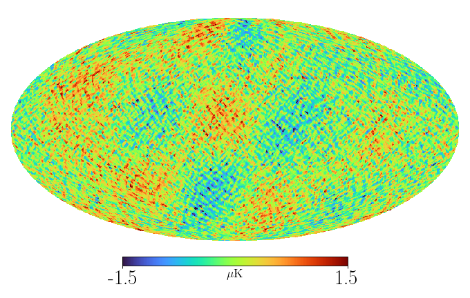
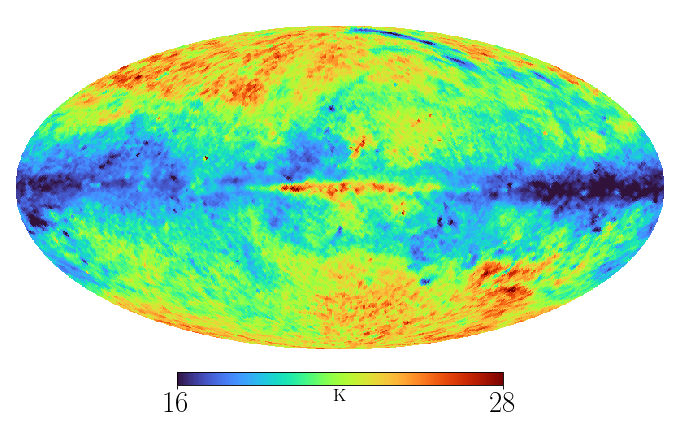
The CMB map was generated using the PySM c1 model. This generates a CMB realisation from a set of unlensed CMB power spectra, $\mathbf{C}_{\ell}=(C_{\ell}^{TT},C_{\ell}^{EE},C_{\ell}^{BB},C_{\ell}^{TE})$, calculated using CAMB (Lewis et al., 2000). A lensed CMB realisation is then computed using nearest-neighbour Taylor interpolation (Næss & Louis, 2013). For our simulated $B$-mode power spectrum we set $r=5\times 10^{-3}$, and assume a delensing fraction of $60\%$, corresponding to the approximate level of delensing expected to be achieved using next-generation CMB experiments (Errard et al., 2016; Challinor et al., 2018). The component amplitude templates and spectral parameter maps used in our simulations are shown in Fig. 1.

Table 1: Frequencies and polarization sensitivities for the C-BASS and LiteBIRD experiments, used in our simulations for algorithm validation. Sensitivities are given in CMB thermodynamic temperature units. Simulated maps were smoothed to a common resolution of $70\,\mathrm{arcmin}$, corresponding to the lowest resolution, $40\,\mathrm{GHz}$ LiteBIRD channel. This resolution is sufficient for targeting multipoles $\ell\lesssim 100$, i.e., angular scales corresponding to the reionization and recombination peaks of the primordial $B$-mode power spectrum.

Experiment	Frequency	Polarization
Name	[GHz]	Sensitivity
		$[\mu\mbox{K${}_{\mathrm{cmb}}$-arcmin}]$
C-BASSa	5	4320
LiteBIRDb	40	27.9
	50	19.6
	60	15.6
	68	12.3
	78	10.0
	89	9.4
	100	7.6
	119	6.4
	140	5.1
	166	7.0
	195	5.8
	235	8.0
	280	9.1
	337	11.4
	402	19.6

• ^aJones et al. (2018)

• ^bSekimoto et al. (2018)

(a) $\textbf{{A}}_{\mathrm{cmb}}^{Q}$

(b) $\textbf{{A}}_{\mathrm{d}}^{Q}$ @ $40\,\mathrm{GHz}$

(c) $\textbf{{A}}_{\mathrm{s}}^{Q}$ @ $402\,\mathrm{GHz}$

(d) $\textbf{{A}}_{\mathrm{cmb}}^{U}$

(e) $\textbf{{A}}_{\mathrm{d}}^{U}$ @ $402\,\mathrm{GHz}$

(f) $\textbf{{A}}_{\mathrm{s}}^{U}$ @ $40\,\mathrm{GHz}$

(g) $\beta_{d}$

(h) $T_{d}$

(i) $\beta_{s}$

Figure 1: Input component parameter maps used in our simulations. The synchrotron and dust amplitude maps are shown here at reference frequencies of $40\,\mathrm{GHz}$ and $402\,\mathrm{GHz}$ respectively. When performing the component separation with C-BASS and LiteBIRD simulations, we set the synchrotron reference frequency to $\nu_{0}=5\,\mathrm{GHz}$.

4 Mean-shift clustering of sky regions

The modelling of spectral parameters in CMB component separation presents a number of challenges. In the face of limited data it can prove difficult to properly constrain spectral parameters. Attempting to allow full pixel-by-pixel variations in the spectral parameters in this situation can result in significant increases in post component separation noise and in the prior dominating the posterior. Given this, one may seek to reduce the number of degrees of freedom in the sky model by fitting for global spectral parameters. However, this approach will inevitably lead to modelling errors that have the potential to bias cosmological measurements made with the derived CMB map (Thorne et al., 2019). These challenges have motivated modelling approaches where spatially uniform spectral parameters are assumed over a set of defined sky regions. These have included regions defined as super-pixels on low Nside Healpix maps, and regions defined according to similarities in their spectral properties (Górski et al., 2005; Stompor et al., 2009; Errard et al., 2011; Stompor et al., 2016; Alonso et al., 2017; Irfan et al., 2019; Khatri, 2019; Thorne et al., 2019). A detailed discussion of the modelling approaches that can be adopted for spectral parameters in these sky regions is given in Sections 5.3 and 5.4. In this section we describe the mean-shift clustering algorithm, implemented in Scikit-Learn (Comaniciu & Meer, 2002; Pedregosa et al., 2011), that we have used to define regions on the sky for our component separation analyses. The mean-shift clustering algorithm has previously been used in Jew & Grumitt (2019) to identify pixels with good detections of the synchrotron spectral index.

We use the mean-shift clustering algorithm to construct sky regions according to their location on the sky and their spectral properties. Specifically, we cluster according to the Cartesian coordinates of pixel centres on the unit sphere, $(x^{1},x^{2},x^{3})$, and the naive spectral indices between the C-BASS $5\,\mathrm{GHz}$ and LiteBIRD $40\,\mathrm{GHz}$ channels, and the LiteBIRD $337\,\mathrm{GHz}$ and $402\,\mathrm{GHz}$ channels in polarized intensity. The two sets of frequency maps are used as synchrotron and thermal dust tracers respectively, with the naive spectral indices in a pixel, $p$, being given by,

$$\beta^{i,j}_{p}=\frac{\ln(m_{i}(p)/m_{j}(p))}{\ln{(\nu_{i}/\nu_{j})}},$$ (4)

where $m_{i}(p)$ and $m_{j}(p)$ are the map values in the pixel $p$, at the frequencies $\nu_{i}$ and $\nu_{j}$ respectively. Given these parameters we may form the feature vector,

$$\textbf{{z}}_{p}=(x^{1}_{p}/\zeta,x^{2}_{p}/\zeta,x^{3}_{p}/\zeta,\beta^{5,40}_{p},\beta^{337,402}_{p}),$$ (5)

where $\zeta$ is a spatial vector scaling factor. Setting the value of $\zeta$ to be less than $1$ allows us to preferentially weight proximity on the sky as being favourable over proximity in spectral index space. The function of the mean-shift algorithm is then to cluster points in this five dimensional feature space.

The mean-shift algorithm proceeds by assigning a walker to each pixel, giving us the starting vectors, $\textbf{{z}}^{0}_{p}=\textbf{{z}}_{p}$. The walkers then step through the feature space towards regions of higher density, with the $t^{\mathrm{th}}$ update being calculated as,

$$\textbf{{z}}^{t}_{p}=\textbf{{z}}^{t-1}_{p}+\textbf{{s}}(\textbf{{z}}^{t-1}_{p}),$$ (6)

where s is the mean-shift vector, given by,

$$\textbf{{s}}(\textbf{{z}}^{t}_{p})=\frac{\sum_{q}K(\textbf{{z}}^{t}_{q}-\textbf{{z}}^{t}_{p})\textbf{{z}}^{t}_{q}}{\sum_{q}K(\textbf{{z}}^{t}_{q}-\textbf{{z}}^{t}_{p})}.$$ (7)

For our purposes we choose the kernel, $K$, to be a top-hat defined by,

$$K(\mathbf{\Delta})=\begin{cases}1,&|\mathbf{\Delta}|\leq\omega,\\ 0,&|\mathbf{\Delta}|>\omega,\end{cases}$$ (8)

where $\omega$ is the bandwidth parameter. Walkers take steps until they converge i.e., walker positions in feature space no longer change with new updates (up to some threshold). Regions are then defined as a set of pixels whose walkers have converged on the same position in the 5-dimensional feature space. Any regions containing fewer pixels than some arbitrary minimum are reassigned to the nearest region in feature space containing a sufficient number of pixels.

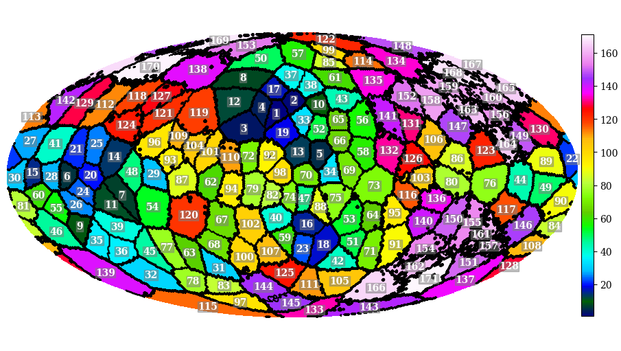
In Fig. 2 we show the regions obtained using the frequency channels outlined above, which are used as the region definitions for the component separation analyses in this paper. We used the simulated maps at a Healpix Nside of 64, setting $\zeta=0.5$, $\omega=0.3$ and the minimum number of pixels in a region to 10 (Górski et al., 2005). Using the foreground tracers and parameters described here, we obtain 171 regions. The smallest region on the sky contains 138 pixels, and the largest region contains 645 pixels. The mean number of pixels in a region is $\langle N_{\mathrm{pix}}\rangle\approx 290$, and the standard deviation in the number of pixels is $\sigma(N_{\mathrm{pix}})\approx 95$. In regions of low signal-to-noise ratio (SNR) the borders of regions become less smooth. This can be mitigated to some extent by defining regions on lower Nside maps, at the cost of the larger pixel size meaning regions become more coarse. Using lower Nside maps can lead to a significant degradation in computational performance when assuming foreground spectral parameters in a given region are related in some manner.

A range of possible, non-trivial, extensions to the clustering algorithm exist that could help to alleviate some of the issues surrounding region definition in areas of the sky with low SNR. Instead of using naive spectral indices as a tracer of the spectral properties of diffuse emission over the sky, a more sophisticated estimation of the spectral indices could be performed, accounting for noise properties across the sky. The spectral index estimation could also be improved with better tracers of synchrotron and thermal dust emission. It is worth noting here that the use of the C-BASS map as a synchrotron template is particularly important. If instead we had only used low frequency LiteBIRD channels as our synchrotron tracers the naive synchrotron spectral index estimates would have been heavily noise dominated. Using the methods outlined here, we found it would only possible to define very coarse regions on Nside=8 maps.

Figure 2: Regions defined using the mean-shift clustering algorithm, produced using Nside=64 maps. We set $\zeta=0.5$, $\omega=0.3$ and the minimum number of pixels in a region to 10. Given our set-up, we obtain 171 regions. The smallest region contains 138 pixels, and the largest region contains 645 pixels. The mean number of pixels is $\langle N_{\mathrm{pix}}\rangle\approx 290$, and the standard deviation of the number of pixels is $\sigma(N_{\mathrm{pix}})\approx 95$. In regions of low SNR we can see that the region borders become less smooth, due to the naive spectral indices used to cluster pixels on the sky becoming contaminated by noise.

5 Parametric Bayesian CMB component separation

We have developed a new implementation of Bayesian pixel-by-pixel CMB component separation, using the NUTS algorithm to explore our parameter space (Hoffman & Gelman, 2014). The primary benefit in using NUTS to sample from the target distribution is in its avoidance of the random walk behaviour that slows more conventional sampling algorithms such as Metropolis-Hastings and Gibbs sampling. The component separation code is written in the Python programming language, with the NUTS algorithm being implemented through the PyMC3 library (Salvatier et al., 2016). In its current form, the whole-sky component separation is parallelized over the sky regions defined using the mean-shift clustering algorithm. For our validation purposes in this paper, we do not consider monopole and dipole corrections, or instrumental factors such as colour corrections in our modelling. The extension of our modelling to include such complications is left to future work.

Bench-marking the algorithm performance against the rate of effective sample generation, NUTS offers potential performance improvements of $\sim 10^{3}$ compared to sampling with Metropolis-Hastings. Close to the Galactic plane sampling becomes more difficult, with the CMB completely sub-dominant to foregrounds. In this situation computational performance can be degraded such that the sampler exhibits undesirable random walk behaviour. By parallelizing over sky regions, and masking the most contaminated sky regions close to the Galactic plane, it should be possible to achieve rapid convergence. We also note that these bench-marking tests have been performed without extensive optimization of the component separation code. By exploring re-parameterizations, model prior choice, optimizing sampling parameters etc. it is likely that we would be able to achieve further performance improvements. It would also be worthwhile considering the potential for GPU acceleration with PyMC3. For the hierarchical model, the posterior exhibits geometrical pathologies that make sampling with non-gradient based algorithms essentially intractable (Betancourt & Girolami, 2015). However, using NUTS we are able to achieve comparable computational performance to the complete pooling model.

The outline of this section is as follows: In Section 5.1 we describe the general sky model and likelihood used in our component separation analysis. In Section 5.2 we give an overview of the NUTS algorithm. In Section 5.3 we discuss the complete pooling model, where we fit for constant spectral parameters over sky regions. In Section 5.4 we discuss our hierarchical modelling approach, where we directly fit for the underlying hyper-distributions of the spectral parameters. In Section 5.5 we describe the convergence checks and diagnostics performed during sampling.

5.1 Sky model and likelihood

In attempting to observe the CMB we actually observe multiple sky components. It is the goal of our component separation to extract the CMB from these additional confusing components. For a given sky pixel, $p$, we may write the observed value in that pixel as,

$$d_{p,\lambda}(\nu)=s_{p,\lambda}(\nu)+n_{p,\lambda}(\nu),$$ (9)

where $\nu$ is the observing frequency, $\lambda=\left\{I,Q,U\right\}$ represents one of the Stokes parameters, $s_{p,\lambda}(\nu)$ is the true sky signal and $n_{p,\lambda}(\nu)$ is the noise term. For our analysis in this paper we restrict ourselves to $\lambda=\left\{Q,U\right\}$.

The true sky signal includes contributions from diffuse emission, compact sources, line emission etc. For our current modelling purposes we focus on diffuse emission, as discussed in Section 2. Additional contributions from compact sources, line emission etc. are important considerations when performing component separation on real experimental data. A variety of strategies exist for mitigating their contribution, e.g. through masking point sources, and direct modelling during the fitting process. However, this sits beyond the scope of our algorithm validation.

The noise term consists largely of contributions from instrumental white noise and $1/f$ noise, which acts to introduce large-scale correlated noise in the sky maps. For ground-based experiments mitigating atmospheric noise is a significant challenge, largely limiting accessible angular scales to $\ell\gtrsim 30$. The ability of such experiments to accurately recover low multipoles will be vital for future $B$-mode experiments (Alonso et al., 2017).

Given a set of sky maps at frequencies $\mathbf{\nu}=\left[\nu_{1},\ldots,\nu_{N}\right]$, the Gaussian likelihood for a pixel, $p$, is given by,

$$-\ln{\mathcal{L}_{p,\lambda}(\mathbf{\Theta}_{p,\lambda})}=\sum_{i}\frac{1}{2}\ln{\left(2\pi\sigma_{p,\lambda}^{2}(\nu_{i})\right)}+\\ \frac{\left(d_{p,\lambda}(\nu_{i})-s_{p,\lambda}(\nu_{i},\mathbf{\Theta}_{p,\lambda})\right)^{2}}{2\sigma_{p,\lambda}^{2}(\nu_{i})},$$ (10)

where $\mathbf{\Theta}_{p,\lambda}$ are the model parameters, and $\sigma_{p,\lambda}$ is the pixel noise. We assume for simplicity that the noise is independent between pixels and frequency channels. This is not necessarily optimal when we consider the complications described above. However, the approximation is sufficient for the purposes of algorithm validation and performing simple forecasting analyses for CMB $B$-mode searches.

5.2 The No-U-Turn Sampler

The key measure of the efficiency of a sampling algorithm is in its ability to produce effective/independent samples, or equivalently reduce the correlation between samples. Indeed, this is where NUTS significantly out-performs standard Metropolis-Hastings and Gibbs sampling algorithms. Even though an individual step in these simpler sampling algorithms is less computationally expensive, their random-walk behaviour results in highly correlated samples and hence very inefficient generation of effective samples. At its core, the NUTS algorithm is an extension of HMC, which was originally developed for performing calculations in lattice field theory (Duane et al., 1987). In this section we give an overview of the HMC algorithm, and the additional tuning procedures NUTS implements to avoid the need for hand-tuned HMC implementations. For a detailed discussion of NUTS and HMC see Hoffman & Gelman (2014); Monnahan et al. (2017); Betancourt (2017); Betancourt et al. (2017).

HMC essentially proceeds by generating physical trajectories through parameter space, akin to simulating particle trajectories through a potential. A simple implementation of HMC may proceed as follows:

1. Given a set of parameters, $\mathbf{\Theta}=\left[\Theta_{1},\ldots,\Theta_{\mathrm{d}}\right]$, with corresponding joint density, $p\left(\mathbf{\Theta}\right)$, we introduce a set of auxiliary momentum variables, $\textbf{{r}}=\left[r_{1},\ldots,r_{\mathrm{d}}\right]$. We take the distribution over the momenta to be a Gaussian distribution centered on zero, i.e., $\textbf{{r}}\sim\mathcal{N}(\mathbf{0},\textbf{{M}})$, where M is the mass matrix. This defines a kinetic energy term,

   $$K(\mathbf{\Theta},\textbf{{r}})=-\ln p(\textbf{{r}}|\mathbf{\Theta})=\frac{1}{2}\textbf{{r}}^{\top}\textbf{{M}}^{-1}\textbf{{r}}+\ln{\left|\textbf{{M}}\right|}+\mathrm{const.}$$ (11)

   We may then define the Hamiltonian of our system as,

   $$\mathcal{H}(\textbf{{r}},\mathbf{\Theta})=-\ln p(\textbf{{r}}|\mathbf{\Theta})-\ln p\left(\mathbf{\Theta}\right)=K(\mathbf{\Theta},\textbf{{r}})+V\left(\mathbf{\Theta}\right),$$ (12)

   where we define the potential energy term, $V\left(\mathbf{\Theta}\right)=-\ln p\left(\mathbf{\Theta}\right)$.

2. We then evolve our position in parameter space by integrating Hamilton’s equations,

   $$\frac{\mathrm{d}\mathbf{\Theta}}{\mathrm{d}t} =\frac{\partial\mathcal{H}}{\partial\textbf{{r}}},$$ (13)

   $$\frac{\mathrm{d}\textbf{{r}}}{\mathrm{d}t} =-\frac{\partial\mathcal{H}}{\partial\mathbf{\Theta}}.$$ (14)

   Practically this is done through a leapfrog algorithm. To generate a new sample in our Markov chain we draw r from $\mathcal{N}(\mathbf{0},\textbf{{M}})$. The leapfrog steps then proceed as,

   $$\textbf{{r}}^{t+\epsilon/2}=\textbf{{r}}^{t}-\frac{\epsilon}{2}\nabla_{\mathbf{\Theta}}V(\mathbf{\Theta}^{t}),$$ (15)

   $$\mathbf{\Theta}^{t+\epsilon}=\mathbf{\Theta}^{t}+\epsilon\textbf{{M}}\textbf{{r}}^{t+\epsilon/2},$$ (16)

   $$\textbf{{r}}^{t+\epsilon}=\textbf{{r}}^{t+\epsilon/2}-\frac{\epsilon}{2}\nabla_{\mathbf{\Theta}}V(\mathbf{\Theta}^{t+\epsilon}),$$ (17)

   where $\epsilon$ is the leapfrog step-size. The leapfrog steps used to update our position have the convenient property of being a symplectic integrator. That is, the numerical trajectory generated by the leapfrog steps preserve the volume of phase space, as is the case for the Hamiltonian trajectories they approximate. A more detailed discussion of the numerical integration of Hamilton’s equations can be found in Leimkuhler & Reich (2004). These leapfrog steps are performed $L$ times to generate a new proposal position, $\left(\mathbf{r}^{*},\mathbf{\Theta}^{*}\right)$.

3. The new proposal position is then accepted with a probability of acceptance given by,

   $$p_{\alpha}=\mathrm{min}\left\{1,\exp\left(\mathcal{H}(\textbf{{r}},\mathbf{\Theta})-\mathcal{H}(\textbf{{r}}^{*},\mathbf{\Theta}^{*})\right)\right\}.$$ (18)

   We note that what we have done here is essentially generate a Metropolis-Hastings proposal step with a very high chance of being accepted.

4. By repeating this sampling procedure $N$ times we may generate the parameter samples for our Markov chain.

The mass matrix used to define the distribution over the momenta acts to rotate and re-scale parameter space. Choosing $\textbf{{M}}^{-1}$ to be the covariance of the target distribution will help to de-correlate the target distribution, which can lead to significant performance improvements when dealing with highly correlated parameters. For practical implementations the mass matrix can be estimated during a tuning phase. Starting with the identity matrix we can generate an initial sample set, from which we update our estimate of the mass matrix using the sample covariance. We may then iterate over this tuning process to generate an accurate estimate of the covariance of the target distribution (Betancourt, 2017). Whilst estimating off-diagonal elements of the mass matrix does help in de-correlating the target distribution, using the off-diagonal elements does not necessarily scale well to high dimensional problems given the need to invert the mass matrix at the end of tuning, and perform matrix multiplications during leapfrog steps. For our analysis in this paper we only tune diagonal elements of the mass matrix. However, this can significantly improve sampling efficiency for single pixel analyses, or analyses assuming complete independence between pixels. In this case, one can employ the tuning steps in Foreman-Mackey et al. (2019), using the default tuning schedule described in Stan Development Team (2012).

The efficiency of HMC as described above critically depends on the choice of $\epsilon$ and $L$ used in the leapfrog steps. If $\epsilon$ is chosen to be too small, the sampler will waste computation taking very small steps along the Hamiltonian trajectories. In contrast, if $\epsilon$ is chosen to be too large, the simulation of the Hamiltonian trajectory will become inaccurate and the sampler will produce proposal steps with low acceptance probabilities. If $L$ is chosen to be too small, the sampler will generate samples close to one another, resulting in undesirable random walk behaviour. If $L$ is chosen to be too large on the other hand, the sampler will generate paths through parameter space that loop back on themselves. This results in proposal steps close to the starting value, with the additional waste of generating the extended trajectory. In even more severe scenarios, a poor choice of $L$ that results in the sampler jumping from one side of parameter space to another at each iteration can result in a non-ergodic chain i.e. a chain that is not guaranteed to converge on the target distribution (Neal, 2012).

The need to finely tune $\epsilon$ and $L$ means that standard implementations of HMC typically require costly tuning runs. This can significantly reduce the utility and general applicability of HMC in realistic problems. The NUTS algorithm overcomes these problems by automatically tuning these sampling parameters. The value of $\epsilon$ is tuned during an initial tuning phase to meet some target acceptance probability. The target acceptance probability can be adjusted depending on the degree of curvature in the posterior, with a higher acceptance rate (or equivalently, smaller step-size) being needed for highly curved distributions. The value of $L$ is modified during sampling to meet a No-U-Turn criterion. That is, the leapfrog integrator is iterated over until the simulated trajectory begins to turn back on itself, or some maximum number of leapfrog simulations are performed. In doing so, the sampler is able to maximize the distance between the proposal step and the initial position, before looping back on itself and wasting computation. Details on these tuning procedures can be found in Hoffman & Gelman (2014); Stan Development Team (2012); Salvatier et al. (2016).

5.3 Complete pooling of spectral parameters

As discussed in Section 4, in the face of limited data and low SNR, allowing spectral parameters to vary completely from pixel to pixel is sub-optimal, resulting in increased levels of post component separation noise and the posterior potentially becoming prior dominated. As a first alternative to allowing full pixel-by-pixel variations we may instead assume spectral parameters to be constant over the regions defined as in Section 4 i.e., we assume a complete pooling of the spectral parameters.

The priors used in the complete pooling model are given in Table 2. We assign informative Normal priors to the spectral parameters. The standard deviations on the priors for $\beta_{\mathrm{s}}$ and $\beta_{\mathrm{d}}$ are chosen to be $0.3$, corresponding to the bandwidth used in clustering sky regions and encompassing most of the range over which these parameters have been measured (Planck Collaboration et al., 2016b; Krachmalnicoff et al., 2018). For the dust temperature we set a prior based on constraints on the dust temperature found in the Planck Commander analysis (Planck Collaboration et al., 2016a, b). These help to down-weight the more extreme regions of parameter space, offering significant computational performance improvements, and helping to regularize the posterior by reducing the biasing effect of the probability mass associated with extreme parameter values. Detailed discussion of prior choice, in particular around the use of weakly informative priors, can be found in Gelman (2006a); Gelman et al. (2008); Evans & Jang (2011); Polson & Scott (2012); Gelman & Hennig (2017); Simpson et al. (2017); Gelman et al. (2017). In addition to the Normal priors on the spectral parameters we multiply these by the associated Jeffreys priors as in the Planck Commander analysis (Jeffreys, 1946, 1961; Eriksen et al., 2008b; Planck Collaboration et al., 2014, 2016a, 2016b).

Table 2: Priors for parameters in the complete pooling model. We assign informative Normal priors to the spectral parameters, and flat priors to the amplitude parameters. In addition to the Normal priors for the spectral parameters, we multiply these by their associated Jeffreys priors as in the Planck Commander analysis. Spectral parameters are assumed to be constant over a given region, whilst amplitude parameters are allowed to vary within each pixel, $p$. We restrict our analysis to polarization, so that $\lambda=\{Q,U\}$.

$\Theta$	$p(\Theta)$
$\beta_{\mathrm{s}}$	$\mathcal{N}(\mu=-3,\sigma=0.3)$
$\beta_{\mathrm{d}}$	$\mathcal{N}(\mu=1.6,\sigma=0.3)$
$T_{\mathrm{d}}$	$\mathcal{N}(\mu=21.0,\sigma=2.0)$
$A_{\mathrm{s}}^{p,\lambda}$	$\mathrm{Unif}(-\infty,\infty)$
$A_{\mathrm{d}}^{p,\lambda}$	$\mathrm{Unif}(-\infty,\infty)$
$A_{\mathrm{cmb}}^{p,\lambda}$	$\mathrm{Unif}(-\infty,\infty)$

Our emission model for a pixel, $p$ in some sky region is given by,

$$s_{p,\lambda}(\nu)=A_{\mathrm{s}}^{p,\lambda}f_{\mathrm{s}}(\nu,\beta_{\mathrm{s}})+A_{\mathrm{d}}^{p,\lambda}f_{\mathrm{d}}(\nu,\beta_{\mathrm{d}},T_{\mathrm{d}})+A_{\mathrm{cmb}}^{p,\lambda}f_{\mathrm{cmb}}(\nu).$$ (19)

The functions, $f_{\mathrm{s}}(\nu,\beta_{\mathrm{s}})$, $f_{\mathrm{d}}(\nu,\beta_{\mathrm{d}},T_{\mathrm{d}})$ and $f_{\mathrm{cmb}}(\nu)$ are the spectral forms of the synchrotron, dust and CMB components, as defined in Section 2. Note that we assume the spectral parameters to be identical for $\lambda=\{Q,U\}$. We model our data as being Normally distributed i.e., we assume the Gaussian likelihood in Equation 10.

Complete pooling offers a potentially effective approach to account for the spatial variation in spectral parameters whilst avoiding the generation of excessive post component separation noise. However, with additional data points at low and/or high frequencies it is possible to adopt a more sophisticated, hierarchical model of the spectral parameters in these regions. It is worth noting that for the complete pooling model one can analytically marginalize over the amplitude parameters as in Alonso et al. (2017). This greatly reduces the dimension of parameter space and hence improves the sampling efficiency. We have not implemented sampling of this marginal distribution for our analysis here, where we study the computational performance of NUTS in sampling the full posterior. Indeed, the intrinsic efficiency of NUTS makes this unnecessary.

5.4 Hierarchical modelling of spectral parameters

In statistical modelling, we often encounter scenarios where our model contains a set of latent variables that are related in some way. In such a scenario it is neither ideal to treat the latent variables as being entirely independent, or to simply fit for a single, global variable. Instead we can take a hierarchical approach. In a hierarchical Bayesian model we introduce a set of population level hyper-parameters, which define the distribution from which our individual latent variables are drawn (Gelman, 2006b; Gelman & Hill, 2007).

In the context of CMB component separation, we may model the pixel spectral parameters within our regions as being drawn from some underlying hyper-distributions. In our particular case we model the spectral parameters as being drawn from underlying Normal distributions, parameterized by the hyper-parameters, $\{(\mu_{\beta_{\mathrm{s}}},\sigma_{\beta_{\mathrm{s}}}),(\mu_{\beta_{\mathrm{d}}},\sigma_{\beta_{\mathrm{d}}}),(\mu_{T_{\mathrm{d}}},\sigma_{T_{\mathrm{d}}})\}$. Each pair corresponds to the mean and standard deviation of the underlying Normal hyper-distribution for the synchrotron spectral index, the dust spectral index and the dust temperature respectively. During component separation we jointly fit for the population-level hyper-parameters and the associated pixel-level spectral parameters. The hierarchical approach allows us to model the pixel-level variations in the spectral parameters, with the hyper-distributions reducing the propensity of the model to overreact to noise, as would be the case if we assumed total independence between pixel-level spectral parameters (Katahira, 2016).

Our emission model takes the same form as in Equation 19, and we again assume the Gaussian likelihood in Equation 10. The priors for our hierarchical model are listed in Table 3. Analogously to the complete pooling model, we set informative priors on the spectral hyper-parameters. For the means of the hyper-distributions we set the same Normal priors as for the spectral parameters in the complete pooling model. For the standard deviations of the hyper-distributions we set Half-Normal priors, with scale parameters set to correspond to the standard deviations of the mean priors. The Half-Normal prior constrains the standard deviations to be positive, with the scale parameters chosen to encapsulate the likely degree of variation of spectral parameters in a given region. Setting informative priors on the hyper-parameters in a hierarchical model can be particularly important in ensuring the robust computational performance of the sampling algorithm. Hyper-parameters are highly correlated with the associated pixel-level parameters, and small changes in the values of the hyper-parameters can induce large changes in the target distribution. This can result in funnel-like geometries in the posterior when the data is limited i.e., a region of high density but low volume below a region of low density but high volume. The funnel regions are highly curved, which can lead to major computational difficulties during sampling, in the worst case leading to a failure in geometric ergodicity. This problem can be partly mitigated through setting informative priors that down-weight more extreme parameter values as we have done here (Gelman, 2006a; Betancourt & Girolami, 2015).

Table 3: Priors for parameters in the hierarchical model. For the means of the spectral hyper-distributions we assign Normal priors, and for the standard deviations of the hyper-distributions we assign Half-Normal priors. The priors for the pixel-level spectral parameters are then defined through their conditional dependence on the hyper-parameters. As with the complete pooling model, we assign flat priors to the amplitude parameters and allow them to vary from pixel to pixel. We restrict our analysis to polarization.

$\Theta$	$p(\Theta)$
$\mu_{\beta_{\mathrm{s}}}$	$\mathcal{N}(\mu=-3,\sigma=0.3)$
$\sigma_{\beta_{\mathrm{s}}}$	$\mbox{Half-Normal}(\sigma=0.35)$
$\mu_{\beta_{\mathrm{d}}}$	$\mathcal{N}(\mu=1.6,\sigma=0.3)$
$\sigma_{\beta_{\mathrm{d}}}$	$\mbox{Half-Normal}(\sigma=0.35)$
$\mu_{T_{\mathrm{d}}}$	$\mathcal{N}(\mu=21,\sigma=2)$
$\sigma_{T_{\mathrm{d}}}$	$\mbox{Half-Normal}(\sigma=2.5)$
$\beta_{\mathrm{s}}^{p}$	$\mathcal{N}(\mu=\mu_{\beta_{\mathrm{s}}},\sigma=\sigma_{\beta_{\mathrm{s}}})$
$\beta_{\mathrm{d}}^{p}$	$\mathcal{N}(\mu=\mu_{\beta_{\mathrm{d}}},\sigma=\sigma_{\beta_{\mathrm{d}}})$
$T_{\mathrm{d}}^{p}$	$\mathcal{N}(\mu=\mu_{T_{\mathrm{d}}},\sigma=\sigma_{T_{\mathrm{d}}})$
$A_{\mathrm{s}}^{p,\lambda}$	$\mathrm{Unif}(-\infty,\infty)$
$A_{\mathrm{d}}^{p,\lambda}$	$\mathrm{Unif}(-\infty,\infty)$
$A_{\mathrm{cmb}}^{p,\lambda}$	$\mathrm{Unif}(-\infty,\infty)$

In addition to our choice of informative priors, we re-parameterize our spectral parameters by introducing the auxiliary variables,

$$\Gamma_{c}^{p}\sim\mathcal{N}(0,1),c=\{\mathrm{s},\mathrm{d},\mathrm{cmb}\}.$$ (20)

In the case of the synchrotron spectral index we may re-express $\beta_{\mathrm{s}}$ as,

$$\beta_{\mathrm{s}}^{p}=\mu_{\beta_{\mathrm{s}}}+\Gamma_{\mathrm{s}}^{p}\sigma_{\beta_{\mathrm{s}}},$$ (21)

with analogous expressions for $\beta_{\mathrm{d}}^{p}$ and $T_{\mathrm{d}}^{p}$. Thus, instead of directly sampling the $\{\beta_{\mathrm{s}}^{p},\beta_{\mathrm{d}}^{p},T_{\mathrm{d}}^{p}\}$, we instead sample a set of Gaussian latent variables and obtain the pixel-by-pixel spectral parameters through a translation and scaling with the hyper-parameters. This is known as the non-centred paramterization and has the convenient effect of reducing correlations between the hyper-parameters and the pixel-level spectral parameters. A detailed discussion of the geometrical pathologies of hierarchical models and practical approaches to their mitigation can be found in Betancourt & Girolami (2015).

5.5 Convergence Checks

Given an infinite number of samples it can be shown the the NUTS algorithm will converge on the target distribution. However, it remains important to perform a number of checks to reassure ourselves of convergence after a finite number of samples. To this end, we output a number of convergence diagnostics that we describe below.

The first covergence diagnostic we output is the Gelman-Rubin statistic (Gelman & Rubin, 1992; Brooks & Gelman, 1998). This compares the variance between multiple, independently initialized chains with the variance within each chain, and is defined as,

$$\hat{R}=\frac{\hat{V}}{\hat{W}},$$ (22)

where $\hat{V}$ is the between-chain variance and $\hat{W}$ is the within chain variance. If convergence has been achieved the between-chain and within-chain variance will be equal. In reality we apply the threshold, $\hat{R}\leq 1.1$ to reassure ourselves that our chains satisfy the necessary geometric ergodicity conditions.

We also output the number of effective samples in each chain, $n_{\mathrm{eff}}$ (Geyer, 1992; Brooks et al., 2011). When sampling from a target distribution using some MCMC algorithm, we may draw a total of $N$ samples, but these samples are not totally independent. The effective sample size provides a measure of the number of independent samples in a chain, defined as,

$$n_{\mathrm{eff}}\equiv\frac{N}{\sum_{t=-\infty}^{\infty}\rho_{t}}=\frac{N}{1+2\sum_{t=1}^{\infty}\rho_{t}},$$ (23)

where $\rho_{t}$ is the auto-correlation within a chain at a lag $t$. Details on the estimation of the auto-correlation can be found in Stan Development Team (2012). The appropriate number of effective samples to be able to properly capture the target distribution is to some extent a question of judgement. However, in Kruschke (2011) a threshold of $\sim 1000$ effective samples is proposed to be confident in expectations calculated with parameter chains. As such, we adopt this as a confidence threshold for our sampling output.

Finally, we also output warnings when divergences occur during sampling. A divergence takes place when the sampler encounters a region of the target distribution where the curvature is too high to be resolved given the tuned step-size. In practice, divergences are detected when the value of the Hamiltonian diverges from its initial value when simulating trajectories through parameter space. This is significant in that divergences can mean that the conditions for geometric ergodicity are not met, and therefore using the resultant chains to construct statistical estimators can lead to biased inferences (Betancourt & Girolami, 2015; Betancourt, 2016, 2017).

6 Algorithm Validation

We validate the component separation algorithm’s performance against the simulated experimental observations described in Section 3. For ease of discussion, we assign the following labels to our three validation sets (i.e., simulation and modelling runs):

• CP(L): The LiteBIRD only analysis, fitting the complete pooling model described in Section 5.3.

• CP(LC): The C-BASS and LiteBIRD analysis, fitting the complete pooling model.

• H(LC): The C-BASS and LiteBIRD analysis, fitting the hierarchical model described in Section 5.4.

In all three validation sets we use regions defined on Nside=64 maps, as described in Section 4, for our spectral modelling. We note here that we do not fit the hierarchical model to the simulation set consisting of just LiteBIRD observations. It was found to be very challenging to control for the occurrence of divergences when fitting the hierarchical model to LiteBIRD only observations, leaving the convergence properties of the resulting MCMC chains suspect. These problems around controlling divergences can be understood when we consider the lack of low frequency channels in LiteBIRD. Given limited available information to constrain synchrotron spectral parameters, the posterior geometry for the hierarchical model becomes extremely difficult to sample. Applying the hierarchical model to LiteBIRD only observations likely requires a careful study of prior choice for model hyper-parameters and extended tuning phases to help mitigate the occurrence of divergences.

The outline of this section is as follows: In Section 6.1 we discuss the CMB amplitude output, in Section 6.2 we present the synchrotron and dust amplitude constraints, in Section 6.3 we discuss constraints on the synchrotron spectral index, and in Section 6.4 we show results for the dust spectral parameters.

6.1 CMB amplitude

The primary output from the NUTS component separation are CMB amplitude maps in $Q$ and $U$. This consists of a set of maps corresponding to individual posterior samples, along with the summary maps of the mean and standard deviation of the amplitude maps. In Fig. 3 we show the mean CMB $Q$ and $U$ amplitude maps obtained for our three validation sets, along with the associated maps of the effective sample size. When using a complete pooling model obvious artefacts can be seen in the recovered CMB amplitude maps near the Galactic plane. This is to be expected, given the bright diffuse emission in these regions makes the extraction of weak CMB signals extremely challenging. When using a hierarchical model, as for the H(LC) set, these artefacts are no longer present. By allowing the model to account for the real variation in spectral parameters in our regions, whilst constraining this variation through the fitted hyper-distributions, we are able to achieve a more accurate foreground removal and thereby remove the biases apparent from assuming constant spectral parameters. Regions of the CMB amplitude maps containing component separation artefacts are well traced by the effective sample size. In regions of low effective sample size ($n_{\mathrm{eff}}\lesssim 1000$), the parameter chains exhibit a high degree of auto-correlation, indicative of the sampler struggling to draw independent posterior samples. Thresholding maps of the effective sample size can be used to construct confidence masks for the CMB amplitude maps, which can be used in combination with standard Galactic emission masks.

(a) CP(L): $\textbf{{A}}_{\mathrm{cmb}}^{Q}$

(b) CP(LC): $\textbf{{A}}_{\mathrm{cmb}}^{Q}$

(c) H(LC): $\textbf{{A}}_{\mathrm{cmb}}^{Q}$

(d) CP(L): $\textbf{{A}}_{\mathrm{cmb}}^{U}$

(e) CP(LC): $\textbf{{A}}_{\mathrm{cmb}}^{U}$

(f) H(LC): $\textbf{{A}}_{\mathrm{cmb}}^{U}$

(g) CP(L): $n_{\mathrm{eff}}^{Q}$

(h) CP(LC): $n_{\mathrm{eff}}^{Q}$

(i) H(LC): $n_{\mathrm{eff}}^{Q}$

(j) CP(L): $n_{\mathrm{eff}}^{U}$

(k) CP(LC): $n_{\mathrm{eff}}^{U}$

(l) H(LC): $n_{\mathrm{eff}}^{U}$

Figure 3: Input and output CMB amplitude maps obtained with the NUTS component separation algorithm. In panels (a) to (f) we show the output $\textbf{{A}}_{\mathrm{cmb}}^{Q/U}$ maps for the various validation sets, and in panels (g) to (l) we show the corresponding maps of the effective sample size. Obvious artefacts can be seen in the output $\textbf{{A}}_{\mathrm{cmb}}^{Q/U}$ maps when using a complete pooling model. This is the result of extremely bright foreground emission dominating over the CMB signal, making the extraction of the CMB signal very challenging. These artefacts are well traced by the effective sample size, being most apparent in bright regions close to the Galactic plane and North Polar Spur. By using a hierarchical model we are able to remove these obvious artefacts from our recovered CMB maps.

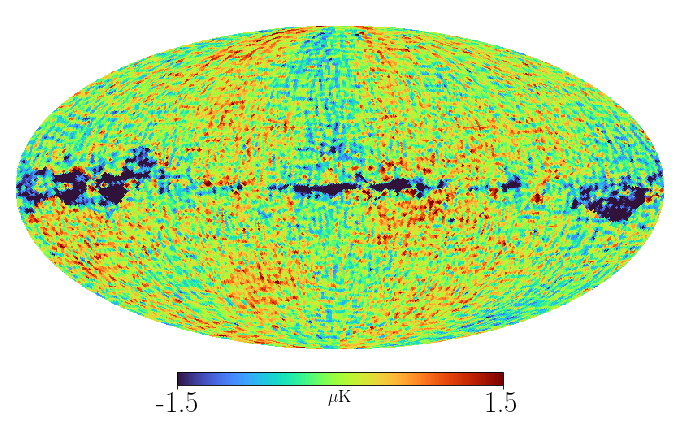
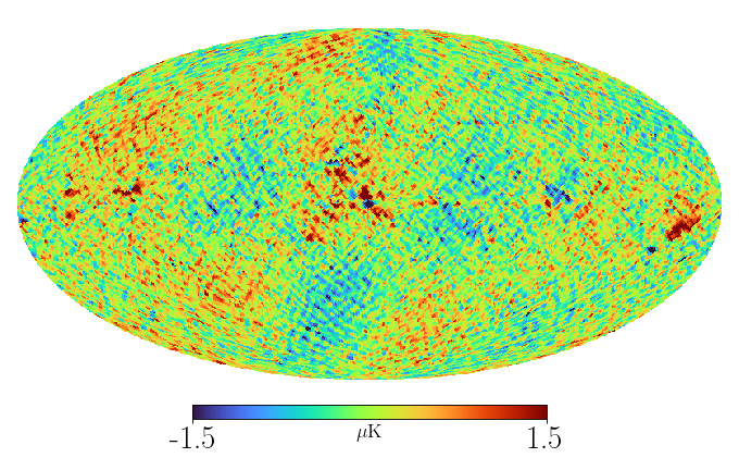
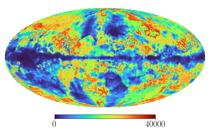
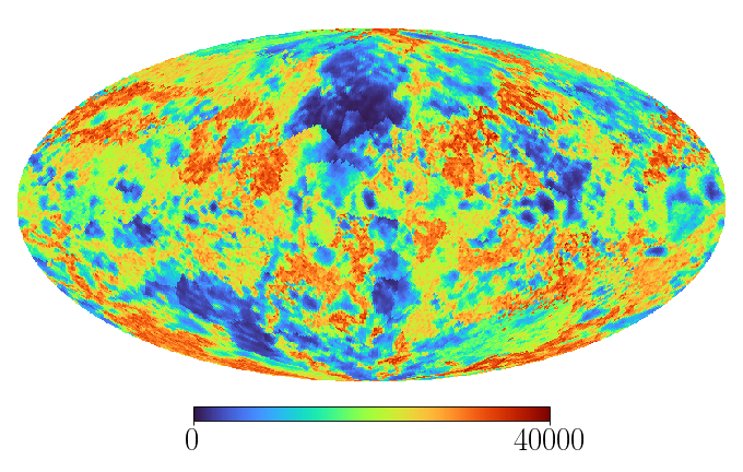
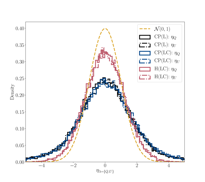
In Fig. 4 we show histograms of the normalized deviations of the $\textbf{{A}}_{\mathrm{cmb}}^{Q/U}$ maps, defined as,

$$\eta_{\lambda}=\frac{\textbf{{A}}_{\mathrm{cmb}}^{\mathrm{in},\lambda}-\textbf{{A}}_{\mathrm{cmb}}^{\mathrm{out},\lambda}}{\sigma_{\mathrm{cmb}}^{\lambda}},\quad\lambda=\{Q,U\},$$ (24)

where $\textbf{{A}}_{\mathrm{cmb}}^{\mathrm{in},Q/U}$ is the input CMB $Q/U$ amplitude map, $\textbf{{A}}_{\mathrm{cmb}}^{\mathrm{out},Q/U}$ is the output CMB $Q/U$ amplitude map, and $\sigma_{\mathrm{cmb}}^{Q/U}$ is the corresponding CMB $Q/U$ standard deviation map. Alongside these histograms we plot the standard Gaussian, $\mathcal{N}(0,1)$. If our observed $\textbf{{A}}_{\mathrm{cmb}}^{\mathrm{out},Q/U}$ are drawn from a Gaussian distribution with mean, $\textbf{{A}}_{\mathrm{cmb}}^{\mathrm{in},Q/U}$ and standard deviation, $\sigma_{\mathrm{cmb}}^{Q/U}$, the normalized deviation should be distributed as a standard Gaussian. The standard deviations of the normalized deviations, calculated using the median absolute deviation (MAD) estimator implemented in astropy (Astropy Collaboration et al., 2013, 2018), are given in Table 4. For the validation sets studied here the distributions of the normalized deviations are slightly wider than the standard Gaussian. This means the uncertainties reported by the CMB amplitude standard deviation maps underestimate the errors on the recovered CMB amplitudes, and the CMB amplitude posterior shows slight departures from Gaussianity. This is not necessarily surprising given the full posterior includes contributions from non-Gaussian priors, and in the case of the hierarchical model contains complex correlations between hyper-parameters and pixel-level parameters.

Validation Set	$\sigma(\eta_{Q})$	$\sigma(\eta_{U})$
CP(L)	1.68	1.67
CP(LC)	1.70	1.72
H(LC)	1.22	1.23

Table 4: Standard deviations of the normalized deviations for the CMB $Q/U$ maps, calculated using the MAD estimator. This estimator avoids some of the sensitivity to outlier values that affects the normal standard deviation estimator. For all three validation sets the distributions of the normalized deviations are slightly wider than the standard Gaussian. This means the uncertainties reported by the standard deviation maps underestimate the errors on the recovered CMB maps, and indicate slight departures from Gaussianity in the marginal CMB amplitude posterior.

Figure 4: Histograms of the normalized deviations of the CMB amplitude maps, obtained for our three validation sets. Alongside these histograms we plot the standard Gaussian, $\mathcal{N}(0,1)$. For all the validation sets, the distributions of the normalized deviations are slightly wider than the standard Gaussian. This indicates slight departures from Gaussianity and that the uncertainties reported by the CMB amplitude standard deviation maps somewhat underestimate the uncertainties on the CMB amplitude.

We perform power spectrum estimation using the NaMaster library (Alonso et al., 2019). NaMaster is a code for performing pseduo-$C_{\ell}$ estimation, accounting for effects from sky masking, as well as performing full $E$ and $B$-mode purification. This is particularly important when the $B$-mode signal is much weaker than the $E$-mode signal, as is the case for CMB $B$-mode studies. In this situation $E$ to $B$ leakage when performing power spectrum estimation on a cut sky can lead to the variance of the $B$-mode power spectrum estimators being dominated by the variance of the leaked $E$-modes. Details on the construction of unbiased pseudo-$C_{\ell}$ estimators, and $E$ and $B$-mode purification can be found in Hivon et al. (2002); Elsner et al. (2017); Alonso et al. (2019).

We generate Galactic emission masks following the procedure in Remazeilles et al. (2018). That is, we extrapolated $10^{\circ}$ smoothed $5\,\mathrm{GHz}$ and $402\,\mathrm{GHz}$ polarized intensity maps to $70\,\mathrm{GHz}$, and applied thresholds against the standard deviation of the $10^{\circ}$ smoothed CMB polarized intensity map at $70\,\mathrm{GHz}$. The $5\,\mathrm{GHz}$ map was extrapolated using a constant spectral index of $\beta_{\mathrm{s}}=-3$ and the $402\,\mathrm{GHz}$ map was extrapolated using a MBB SED, setting $\beta_{\mathrm{d}}=1.6$ and $T_{\mathrm{d}}=19.4\,\mathrm{K}$. We further mask all pixels with $n_{\mathrm{eff}}\lesssim 1000$ in either the $Q$ or $U$ maps, although most of these pixels are already contained within the Galactic emission masks. For the H(LC) set we apply a Galactic emission mask covering approximately $25\%$ of the sky. For the CP(L) and CP(LC) sets we found that a Galactic emission mask covering approximately $60\%$ of the sky was needed to remove the most significant component separation artefacts. Even with the aggressive masking, foreground residuals remained in the recovered power spectra as discussed below.

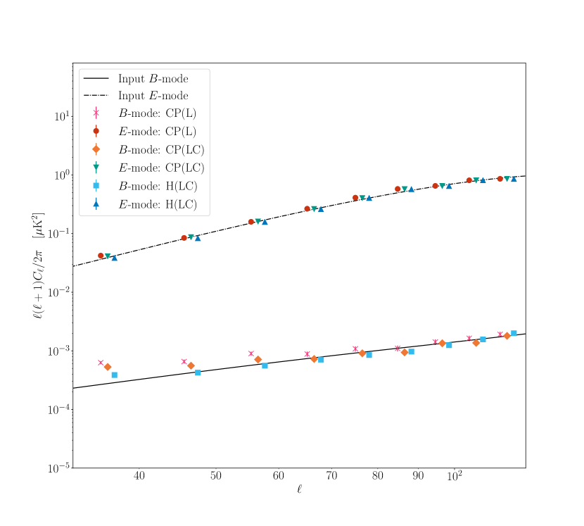
In Fig. 5 we show the $E$ and $B$-mode power spectra derived for the three validation sets, corrected for noise bias. We show power spectra, covering multipoles $32\leq\ell\leq 121$, using a bin width of $\Delta\ell=10$. For lower multipoles, one can obtain better power spectrum estimates by directly sampling the $C_{\ell}$ from the joint distribution, $P(C_{\ell},\textbf{{A}}_{\mathrm{cmb}}|\mathbf{d})$, as is performed in the Commander component separation code (Wandelt et al., 2004; Eriksen et al., 2004; Eriksen et al., 2008a; Taylor et al., 2008). We leave the implementation of this additional power spectrum estimation technique to future work. For multipoles $\ell\gtrsim 121$ the $B$-mode power spectrum estimates became dominated by noise. Given the $70\,\mathrm{arcmin}$ resolution the maps were smoothed to, this is not surprising. At these small scales the beam correction applied during power spectrum estimation begins to inflate the noise present in the CMB amplitude maps.

The noise bias was estimated by calculating the power spectra of $1000$ realizations of the CMB $Q/U$ noise maps. The noise realizations were obtained by taking the difference between individual CMB amplitude posterior samples and the mean CMB amplitude map, i.e.,

$$\delta\textbf{{A}}_{\mathrm{cmb}}^{k,\lambda}=\textbf{{A}}_{\mathrm{cmb}}^{k,\lambda}-\langle\textbf{{A}}_{\mathrm{cmb}}^{\lambda}\rangle,\quad\lambda=\{Q,U\},$$ (25)

where $k$ denotes the $k^{\mathrm{th}}$ posterior sample. The mean value within each multipole bin was taken as the noise bias. The mean CMB power spectrum estimate was then given by the power spectrum estimated from the mean CMB $Q/U$ amplitude maps, minus the estimated noise bias. The covariance matrix was estimated by calculating the power spectra of $1000$ signal plus noise simulations. For the signal simulations we generated $1000$ realizations of the theoretical input CMB power spectrum to account for cosmic variance.

The $E$-mode power spectrum is obtained with high accuracy, confirming the overall fidelity of the component separation algorithm. The recovery of the $B$-mode power spectrum is more challenging, given this signal is significantly weaker than the $E$-mode signal and potentially sub-dominant to foregrounds over most of the sky, at all frequencies. It can be seen that when using a complete pooling model the recovered $B$-mode power spectrum contains large scale foreground residuals, biasing the power spectrum high. This is despite a more aggressive mask being applied when estimating power spectra for the complete pooling model. In real experimental applications one could attempt to mitigate this by applying even more aggressive Galactic emission masks, although this comes at the cost of increasing the uncertainty in the recovered power spectra.

To quantify this bias, we can study the tensor-to-scalar ratio constraints that would be obtained from these power spectra. To do this we approximate the likelihood for the CMB power spectra as a multivariate Gaussian,

$$-2\ln\mathcal{L}=\mathrm{const.}+\sum_{\ell\ell^{\prime}}\left(\tilde{C}_{\ell}-\tilde{C}_{\ell}^{\mathrm{th}}\right)(\Sigma^{-1})_{\ell\ell^{\prime}}\left(\tilde{C}_{\ell^{\prime}}-\tilde{C}_{\ell^{\prime}}^{\mathrm{th}}\right).$$ (26)

The $\tilde{C}_{\ell}$ are the binned power spectra or bandpowers, with $\tilde{C}_{\ell}^{\mathrm{th}}$ being the corresponding theoretical bandpowers, and $\Sigma$ is the bandpower covariance matrix. The sum here runs over the effective $\ell$ values for each bin. It is worth noting that, in general, the CMB likelihood is non-Gaussian. However, for the higher multipoles we consider here the power spectrum estimates are formed by averaging over the individual $a_{\ell m}$’s corresponding to a given multipole, justifying the use of the Gaussian approximation through the central limit theorem.

We parameterize the theoretical power spectrum as,

$$C_{\ell}^{\mathrm{th}}=\frac{r}{0.01}C_{\ell}^{BB}(r=0.01)+A_{L}C_{\ell}^{\mathrm{lens}},$$ (27)

where $A_{L}$ is the lensing amplitude, $C_{\ell}^{BB}(r=0.01)$ is a fiducial primordial $B$-mode power spectrum corresponding to $r=0.01$, and $C_{\ell}^{\mathrm{lens}}$ is the fiducial lensing $B$-mode power spectrum. In a general $B$-mode analysis we would fit jointly for $r$ and $A_{L}$. However, it is challenging to constrain $A_{L}$ solely through the $B$-mode power spectrum here. In a realistic experiment, tight constraints can be put on the lensing $B$-mode through analysis of the $E$-mode, $TE$ correlations and the lensing potential power spectrum. Combined with constraints from external data sets and delensing, one can expect to be able to place a tight prior on $A_{L}$. For the sake of simplicity here, we fix $A_{L}$ to the input value of $0.4$.

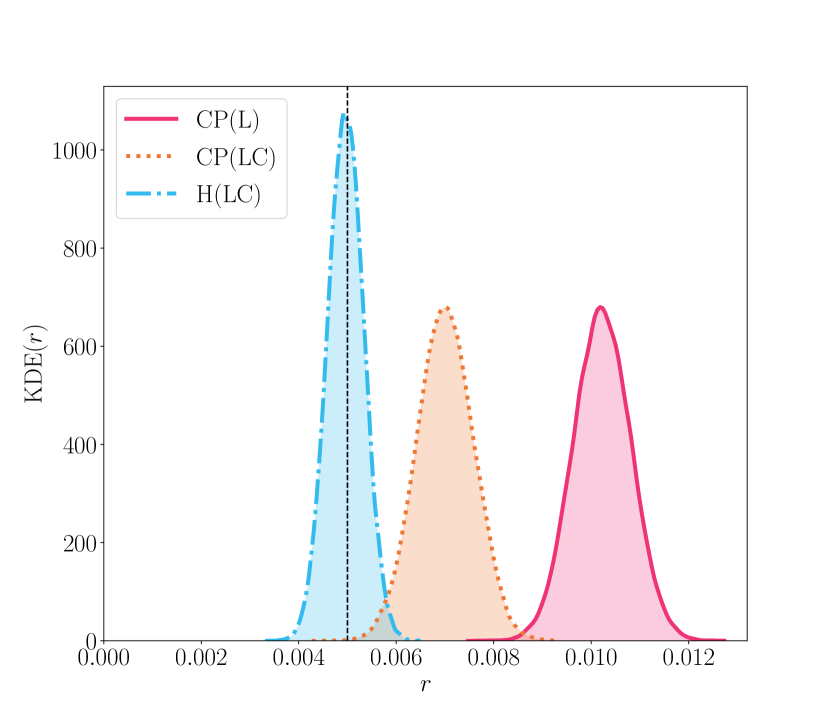
Sampling from this likelihood using PyMC3, we obtain the constraints on $r$ shown in Fig. 6. Using the complete pooling model we recover biased estimates of the tensor-to-scalar ratio, obtaining $r=(10\pm 0.6)\times 10^{-3}$ for the CP(L) set and $r=(7.0\pm 0.6)\times 10^{-3}$ for the CP(LC) set. This can be understood when we consider the large residuals and artefacts present in the recovered CMB when using a complete pooling model. By comparison, the bias is effectively removed for the H(LC) set, obtaining $r=(5.0\pm 0.4)\times 10^{-3}$. It is worth noting that, despite the increased degrees of freedom in using a hierarchical model, the uncertainties obtained for the H(LC) set are smaller than those for the CP(LC) set. This is in large part a result of the smaller Galactic emission mask we are able to adopt for power spectrum estimation with the hierarchical model. By adopting a multi-level structure for the spectral parameters in each region we prevent the model from overreacting to noise, whilst still capturing the spatial variation in spectral parameters. This in turn removes many of the foreground residuals present in the CMB amplitude maps obtained with the complete pooling model.

As an aside, we do caution against interpreting these results as direct forecasts for the proposed LiteBIRD experiment (and/or some combination with additional experiments). LiteBIRD will also obtain constraints on lower multipoles around the reionization peak in the $B$-mode power spectrum, which we have not considered here, increasing the sensitivity of any tensor-to-scalar ratio measurement. Further, for simplicity in this validation analysis we smoothed all channels to the $70\,\mathrm{arcmin}$ resolution of the lowest frequency LiteBIRD channel. This is likely a somewhat pessimistic approach. However, it is beyond the scope of this work to study the impact of the lower resolution of the low frequency LiteBIRD channels on the ability to recover the CMB power spectra at higher multipoles. We have also not considered the effect of mis-modelling foreground SEDs or the impact of experimental systematics, both of which would significantly complicate any $B$-mode measurements. For the discussion here, it was sufficient to consider these simple simulations to study the biases induced through assuming the complete pooling of spectral parameters during component separation.

Figure 5: CMB $E$-mode and $B$-mode power spectra for our three validation sets, covering the multipole range, $32\leq\ell\leq 121$. Power spectra are binned, using a bin width of $\Delta\ell=10$. We plot the power for the three validation sets together, slightly offset from one another for display purposes. The central point within each triple is at the effective multipole value for that bin. We can see that the $E$-mode power spectrum is recovered with high accuracy, demonstrating the overall fidelity of the algorithm. For the $B$-mode power spectrum we can see the results obtained using a complete pooling model contain significant large scale foreground residuals, that are not present when using the hierarchical model.

Figure 6: Tensor-to-scalar ratio constraints obtained for the three validation sets, using derived power spectra over the range $32\leq\ell\leq 121$ and assuming a multivariate Gaussian likelihood. For the CP(L) set we find $r=(10\pm 0.6)\times 10^{-3}$, for the CP(LC) set we find $r=(7.0\pm 0.6)\times 10^{-3}$, and for the H(LC) set we find $r=(5.0\pm 0.4)\times 10^{-3}$. With the addition of C-BASS we see a reduction in the bias on $r$ with the complete pooling model, although a $\sim 3\sigma$ bias still remains for the CP(LC) set. This bias is removed when using a hierarchical model. The uncertainty on the measured tensor-to-scalar ratio is smaller for the hierarchical model because of the smaller Galactic emission mask we are able to adopt for power spectrum estimation.

6.2 Synchrotron and dust amplitudes

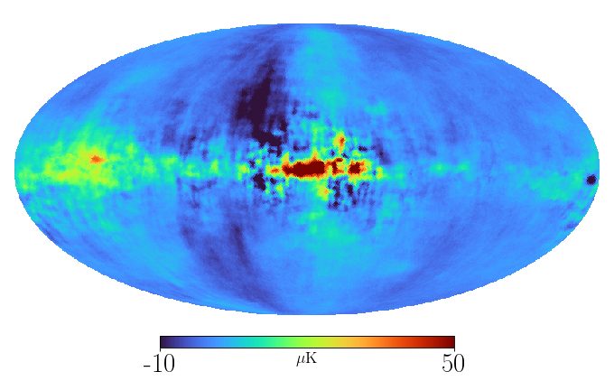
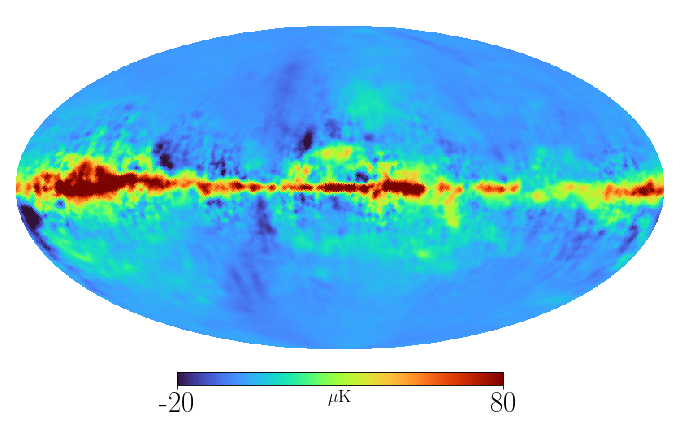
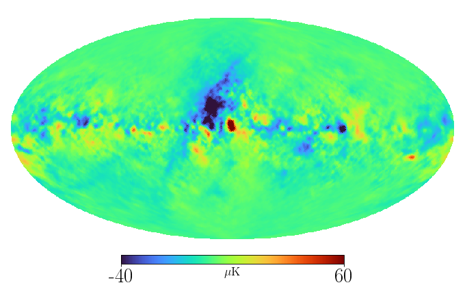
In Fig. 7 we show the dust and synchrotron amplitude maps. Dust amplitude maps are shown at the reference frequency of $\nu_{0}=402\,\mathrm{GHz}$ for all three validation sets. Synchrotron amplitude maps are shown at a reference frequency of $\nu_{0}=40\,\mathrm{GHz}$ for the CP(L) validation set, and at $\nu_{0}=5\,\mathrm{GHz}$ for the CP(LC) and H(LC) validation sets. In all cases we can see the recovered component amplitude maps trace the input component amplitude maps well. However, this is to some extent a result of our choice of reference frequency, with the amplitudes being constrained by the pixel values at those frequencies. The overall level of residuals in the synchrotron amplitude maps is reduced by $\sim 5\%$ for the H(LC) set compared to the CP(LC) set, and the overall residuals in the dust amplitude maps are reduced by $\sim 40\%$. These reductions were estimated using the MAD estimator for the standard deviations of the residuals. Whilst the absolute value of these reductions is small at synchrotron and dust frequencies, they ultimately propagate through to significant biases in the recovered CMB maps, as seen in our tensor-to-scalar ratio estimates.

(a) CP(L): $\textbf{{A}}_{\mathrm{s}}^{Q}$ @ $40\,\mathrm{GHz}$

(b) CP(LC): $\textbf{{A}}_{\mathrm{s}}^{Q}$ @ $5\,\mathrm{GHz}$

(c) H(LC): $\textbf{{A}}_{\mathrm{s}}^{Q}$ @ $5\,\mathrm{GHz}$

(d) CP(L): $\textbf{{A}}_{\mathrm{s}}^{U}$ @ $40\,\mathrm{GHz}$

(e) CP(LC): $\textbf{{A}}_{\mathrm{s}}^{U}$ @ $5\,\mathrm{GHz}$

(f) H(LC): $\textbf{{A}}_{\mathrm{s}}^{U}$ @ $5\,\mathrm{GHz}$

(g) CP(L): $\textbf{{A}}_{\mathrm{d}}^{Q}$ @ $402\,\mathrm{GHz}$

(h) CP(LC): $\textbf{{A}}_{\mathrm{d}}^{Q}$ @ $402\,\mathrm{GHz}$

(i) H(LC): $\textbf{{A}}_{\mathrm{d}}^{Q}$ @ $402\,\mathrm{GHz}$

(j) CP(L): $\textbf{{A}}_{\mathrm{d}}^{U}$ @ $402\,\mathrm{GHz}$

(k) CP(LC): $\textbf{{A}}_{\mathrm{d}}^{U}$ @ $402\,\mathrm{GHz}$

(l) H(LC): $\textbf{{A}}_{\mathrm{d}}^{U}$ @ $402\,\mathrm{GHz}$

Figure 7: Synchrotron and dust amplitude maps obtained for the three validation sets. In panels (a) to (f) we show the synchrotron amplitude maps, shown at the reference frequency of $\nu_{0}=40\,\mathrm{GHz}$ for the CP(L) validation set, and $\nu_{0}=5\,\mathrm{GHz}$ for the CP(LC) and H(LC) validation sets. In panels (g) to (l) we show the dust amplitude maps, displayed at the reference frequency of $\nu_{0}=402\,\mathrm{GHz}$. In all three cases the component separation algorithm recovers accurate estimates of the foreground amplitude maps at their reference frequencies. This is to be expected, and is to some extent a result of our choice of synchrotron and dust reference frequencies. The typical residuals in synchrotron amplitude maps are $\sim 5\%$ lower for the H(LC) set compared to the CP(LC) set. Similarly, the dust amplitude residuals are $\sim 40\%$ lower for the H(LC) set compared to the CP(LC) set.

6.3 Synchrotron spectral parameters

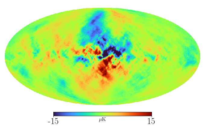
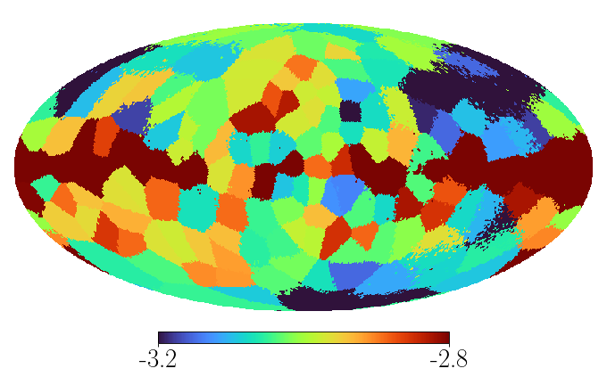
In Fig. 8 we show the synchrotron spectral indices obtained for the three validation sets. In the case of the CP(L) set, we struggle to place accurate constraints on the synchrotron spectral index. This is to be expected, given the lack of low frequency channels below $40\,\mathrm{GHz}$, and is consistent with expectations from the single-pixel component separation analysis presented in Jew et al. (2019). For the CP(LC) validation set, we are able to place improved constraints on the synchrotron spectral index, with the variations in the synchrotron spectral index from region to region tracing the variations in the input spectral index map shown in Fig. 1.

When using a hierarchical model we are able to more finely model variations in the synchrotron spectral index across the sky. As can be seen in panel (c) of Fig. 8, the spectral index in regions of high SNR traces the same variations seen in the input synchrotron spectral index map. In regions of low SNR, away from the Galactic plane, we do see additional small scale features not present in the input $\beta_{s}$ map. This is a result of the noisier estimates of the synchrotron spectral index we obtain in these regions. However, these noisy variations are constrained by the hyper-distribution, which penalises individual estimates of $\beta_{s}$ being too far from the population mean, $\mu_{\beta_{s}}$. Further, even in these noisier regions of the sky we can see that many of the large scale variations in the spectral index are still traced by the individual spectral indices. This is a well known property of hierarchical models, known as posterior shrinkage, and is one of the main advantages of adopting the hierarchical approach i.e., we obtain improved point estimates of our latent variables (Katahira, 2016). For the simulations we have considered here, the overall residuals in the synchrotron spectral index maps are similar between the CP(LC) and H(LC) validation sets. This is partly a result of the input synchrotron spectral index map being highly idealized, lacking in small-scale features (Krachmalnicoff et al., 2018). In realistic scenarios the additional small-scale features in the synchrotron spectral index map will result in more significant mis-modelling errors with the complete pooling model.

(a) CP(L): $\beta_{s}$

(b) CP(LC): $\beta_{s}$

(c) H(LC): $\beta_{s}$

Figure 8: Synchrotron spectral index maps obtained for the three validation sets. For the CP(L) set, we struggle to accurately constrain the synchrotron spectral index, due to the absence of low frequency channels below $40\,\mathrm{GHz}$. With the addition of a $5\,\mathrm{GHz}$ C-BASS channel for the CP(LC) and H(LC) sets, we are able to place improved constraints on the synchrotron spectral index. By allowing for additional pixel-level variations in the spectral index with the hierarchical model, constrained in each region by the fitted hyper-distribution, we are able to better trace the morphology of variations in the synchrotron spectral index. Over the whole sky, the typical residual level is comparable between the CP(LC) and H(LC) validation sets. However, the performance of the complete pooling model is exaggerated somewhat by our simulations, given the lack of small-scale features in the input synchrotron spectral index map.

6.4 Dust spectral parameters

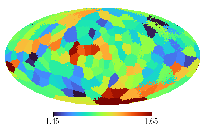
Most of the constraining power for dust spectral parameters comes from high frequency channels i.e., $\nu\gtrsim 100\,\mathrm{GHz}$. In our three validation sets these remained identical, being the high frequency LiteBIRD channels. In Jew et al. (2019) it was found that, given a LiteBIRD-like frequency coverage, it is difficult to constrain dust spectral parameters. Indeed, this was the case for our own analysis here, where informative priors were needed on the dust spectral parameters. The difficulty in constraining dust spectral parameters is reflected in their low effective sample size, which was typically $\lesssim 1000$ over much of the sky in all three validation sets.

In using a hierarchical model for the dust spectral parameters, we are able to fit for variations in the spectral parameters in regions of high SNR close to the Galactic plane. Away from the Galactic plane, the individual variations become much smaller in each region, with the resulting maps of $\beta_{d}$ and $T_{d}$ very obviously tracing out the crude structure of the regions used in the component separation. Given the limited frequency coverage, there is simply not enough information to constrain the low level variations of the dust spectral parameters in each region. In this case the marginal distributions for $\sigma_{\beta_{\mathrm{d}}}$ and $\sigma_{T_{\mathrm{d}}}$ have a large fraction of their probability mass close to zero, constraining individual spectral parameters to be very close to their population means, $\mu_{\beta_{d}}$ and $\mu_{T_{d}}$. The overall residuals for the dust spectral index maps are reduced by $\sim 30\%$ for the H(LC) set compared to the CP(LC) set. The overall residuals in the recovered dust temperature maps are $\sim 25\%$ lower for the H(LC) set compared to the CP(LC) set. By allowing for some of the low-level variations in the dust spectral parameters we are able to obtain smaller residuals in the recovered parameter maps, propagating through to reduced biases in the CMB amplitude estimates.

(a) CP(L): $\beta_{d}$

(b) CP(LC): $\beta_{d}$

(c) H(LC): $\beta_{d}$

(d) CP(L): $T_{d}$

(e) CP(LC): $T_{d}$

(f) H(LC): $T_{\mathrm{d}}$

Figure 9: Dust spectral parameter maps obtained for the three validation sets. Given LiteBIRD-like frequency coverage we struggle to constrain dust spectral parameters for all three validation sets, reflected in low effective sample sizes for the dust spectral parameters. By using a hierarchical model we are able to capture some of the low-level variations in the dust spectral parameters. Across the whole sky, the level of residuals in the dust spectral index map is reduced by $\sim 30\%$ between the CP(LC) and H(LC) validation sets. For the dust temperature maps the level of residuals is reduced by $\sim 25\%$ between the CP(LC) and H(LC) validation sets.

7 Conclusions

We have developed a new implementation of Bayesian CMB component separation, using the NUTS algorithm to draw samples from the full posterior distribution. The NUTS algorithm is a self-tuning variant of HMC, that avoids the random walk behaviour that leads to slow convergence when using standard Metropolis-Hastings and Gibbs sampling algorithms. Measured against the rate of effective sample generation, NUTS offers performance improvements of $\sim 10^{3}$ compared to Metropolis-Hastings when fitting the complete pooling model. Geometrical pathologies typical of hierarchical models often make variants of HMC the only reliable option for the diagnosis of divergences and biased inferences (Betancourt & Girolami, 2015).

We apply this component separation algorithm to simulations of the LiteBIRD and C-BASS experiments to validate the algorithm performance and fidelity. These simulations use a tensor-to-scalar ratio of $r=5\times 10^{-3}$ and a lensing amplitude of $A_{L}=0.4$. Component separation is performed over a set of separate sky regions, defined using the mean-shift algorithm. This clusters sky regions according to the similarity in their synchrotron and dust spectral properties, and their location on the sky. In each region we adopt two different modelling approaches, namely complete pooling and a hierarchical model. In the complete pooling model we assume the spectral parameters in each region are constant. In the hierarchical model we assume spectral parameters are drawn from underlying Gaussian distributions, fitting for the hyper-parameters defining the mean and variance of the Gaussian hyper-distributions, along with the individual pixel-by-pixel spectral parameters constrained by these hyper-distributions.

When using the complete pooling model we are able to recover accurate estimates of the CMB over much of the sky. However, component separation artefacts are present close to the Galactic plane where the CMB is highly sub-dominant to foregrounds. Using the hierarchical model, these artefacts are removed from the recovered CMB. Estimating the CMB power spectra with these maps, we find the complete pooling model induces large scale foreground residuals in the recovered power spectra. Using multipoles between $32\leq\ell\leq 121$ and fixing the lensing amplitude, we are able to translate these power spectrum estimates into tensor-to-scalar ratio constraints. With only LiteBIRD frequency channels, and using the complete pooling model, we find $r=(10\pm 0.6)\times 10^{-3}$. Applying the complete pooling model with an additional C-BASS channel at $5\,\mathrm{GHz}$ we find $r=(7.0\pm 0.6)\times 10^{-3}$, and using the hierarchical model with C-BASS and LiteBIRD we find $r=(5.0\pm 0.4)\times 10^{-3}$. The addition of C-BASS reduces the bias in the recovered tensor-to-scalar ratio for the complete pooling model, however the crude assumptions made regarding the behaviour of spectral parameter still leaves a $\sim 3\sigma$ bias in the estimate of $r$. We find that the hierarchical model offers an effective generative approach to the modelling of spectral parameters, that helps to mitigate the propensity for fitting outliers when assuming total independence between spectral parameters. Further, with the hierarchical model we are able to use a smaller Galactic emission mask in our power spectrum estimation, resulting in a smaller uncertainty on the recovered tensor-to-scalar ratio.

For the analysis in this paper we have developed a simple proof-of-concept implementation of our algorithm. Potential future work includes the extension of the algorithm to allow for the joint fitting of dipole and monopole corrections, along with instrumental effects such as bandpass corrections. It would also be prudent to extend the power spectrum estimation, to include the direct joint sampling of CMB amplitudes and power spectra at low multipoles, and expand the code to allow for multi-resolution analyses. From the perspective of modelling, one may also consider more sophisticated approaches to clustering. For the purposes of validation in this study we used naive spectral indices as tracers of the foreground spectral properties, which will be contaminated by noise. In future work, it would be worthwhile examining improvements in region definition by using more sophisticated estimators of foregrounds spectral properties, along with studying the optimal datasets to be used as foreground templates. Finally, significant gain can potentially be made by exploring optimizations to the component separation code e.g., through re-parameterizations and GPU acceleration.

References

- Abazajian et al. (2016) Abazajian K. N., et al., 2016, arXiv e-prints, p. arXiv:1610.02743
- Ade et al. (2019) Ade P., et al., 2019, J. Cosmology Astropart. Phys., 2019, 056
- Alonso et al. (2017) Alonso D., Dunkley J., Thorne B., Næss S., 2017, Phys. Rev. D, 95, 043504
- Alonso et al. (2019) Alonso D., Sanchez J., Slosar A., LSST Dark Energy Science Collaboration 2019, MNRAS, 484, 4127
- Astropy Collaboration et al. (2013) Astropy Collaboration et al., 2013, A&A, 558, A33
- Astropy Collaboration et al. (2018) Astropy Collaboration et al., 2018, AJ, 156, 123
- BICEP2 Collaboration et al. (2018) BICEP2 Collaboration et al., 2018, Phys. Rev. Lett., 121, 221301
- BICEP2/Keck Collaboration et al. (2015) BICEP2/Keck Collaboration et al., 2015, Phys. Rev. Lett., 114, 101301
- Bennett et al. (2013) Bennett C. L., et al., 2013, The Astrophysical Journal Supplement Series, 208, 20
- Betancourt (2016) Betancourt M., 2016, arXiv e-prints, p. arXiv:1604.00695
- Betancourt (2017) Betancourt M., 2017, arXiv e-prints, p. arXiv:1701.02434
- Betancourt & Girolami (2015) Betancourt M. J., Girolami M., 2015, in Upadhyay S. K., Singh U., Dey D. K., Loganathan A., eds, , Current Trends in Bayesian Methodology with Applications. Chapman and Hall/CRC, New York, Chapt. 4
- Betancourt et al. (2017) Betancourt M., Byrne S., Livingstone S., Girolami M., 2017, Bernoulli, 23, 2257
- Betoule et al. (2009) Betoule M., Pierpaoli E., Delabrouille J., Le Jeune M., Cardoso J. F., 2009, A&A, 503, 691
- Brooks & Gelman (1998) Brooks S. P., Gelman A., 1998, Journal of Computational and Graphical Statistics, 7, 434
- Brooks et al. (2011) Brooks S., Gelman A., Jones G., Meng X.-L., 2011, Handbook of Markov Chain Monte Carlo. CRC press
- Carpenter et al. (2017) Carpenter B., et al., 2017, Journal of Statistical Software, 76
- Challinor et al. (2018) Challinor A., et al., 2018, J. Cosmology Astropart. Phys., 2018, 018
- Chluba et al. (2017) Chluba J., Hill J. C., Abitbol M. H., 2017, MNRAS, 472, 1195
- Comaniciu & Meer (2002) Comaniciu D., Meer P., 2002, IEEE Transactions on Pattern Analysis and Machine Intelligence, 24, 603
- Davies et al. (2006) Davies R. D., Dickinson C., Banday A. J., Jaffe T. R., Górski K. M., Davis R. J., 2006, MNRAS, 370, 1125
- Delabrouille et al. (2003) Delabrouille J., Cardoso J. F., Patanchon G., 2003, MNRAS, 346, 1089
- Dickinson et al. (2018) Dickinson C., et al., 2018, New Astronomy Reviews, 80, 1
- Dodelson (2003) Dodelson S., 2003, Modern cosmology
- Draine & Hensley (2016) Draine B. T., Hensley B. S., 2016, ApJ, 831, 59
- Duane et al. (1987) Duane S., Kennedy A., Pendleton B. J., Roweth D., 1987, Physics Letters B, 195, 216
- Dunkley et al. (2009) Dunkley J., et al., 2009, AIP Conference Proceedings, 1141, 222
- Elsner et al. (2017) Elsner F., Leistedt B., Peiris H. V., 2017, MNRAS, 465, 1847
- Eriksen et al. (2004) Eriksen H. K., et al., 2004, ApJS, 155, 227
- Eriksen et al. (2008a) Eriksen H. K., Jewell J. B., Dickinson C., Banday A. J., Górski K. M., Lawrence C. R., 2008a, ApJ, 676, 10
- Eriksen et al. (2008b) Eriksen H. K., Jewell J. B., Dickinson C., Banday A. J., Górski K. M., Lawrence C. R., 2008b, The Astrophysical Journal, 676, 10
- Errard et al. (2011) Errard J., Stivoli F., Stompor R., 2011, Phys. Rev. D, 84, 063005
- Errard et al. (2016) Errard J., Feeney S. M., Peiris H. V., Jaffe A. H., 2016, J. Cosmology Astropart. Phys., 2016, 052
- Evans & Jang (2011) Evans M., Jang G. H., 2011, Statist. Sci., 26, 423
- Fixsen (2009) Fixsen D. J., 2009, ApJ, 707, 916
- Foreman-Mackey et al. (2019) Foreman-Mackey D., Barentsen G., Barclay T., 2019, dfm/exoplanet: exoplanet v0.1.4, doi:10.5281/zenodo.2561395, https://doi.org/10.5281/zenodo.2561395
- Gelfand & Smith (1990) Gelfand A. E., Smith A. F. M., 1990, Journal of the American Statistical Association, 85, 398
- Gelman (2006a) Gelman A., 2006a, Bayesian Anal., 1, 515
- Gelman (2006b) Gelman A., 2006b, Technometrics, 48, 432
- Gelman & Hennig (2017) Gelman A., Hennig C., 2017, Journal of the Royal Statistical Society: Series A (Statistics in Society), 180, 967
- Gelman & Hill (2007) Gelman A., Hill J., 2007, Data analysis using regression and multilevel/hierarchical models. Vol. Analytical methods for social research, Cambridge University Press, New York
- Gelman & Rubin (1992) Gelman A., Rubin D. B., 1992, Statistical Science, 7, 457
- Gelman et al. (2008) Gelman A., Jakulin A., Pittau M. G., Su Y.-S., 2008, Ann. Appl. Stat., 2, 1360
- Gelman et al. (2017) Gelman A., Simpson D., Betancourt M., 2017, Entropy, 19, 555
- Geyer (1992) Geyer C. J., 1992, Statist. Sci., 7, 473
- Górski et al. (2005) Górski K. M., Hivon E., Banday A. J., Wandelt B. D., Hansen F. K., Reinecke M., Bartelmann M., 2005, ApJ, 622, 759
- Guzmán et al. (2011) Guzmán A. E., May J., Alvarez H., Maeda K., 2011, A&A, 525, A138
- Hanany et al. (2019) Hanany S., et al., 2019, in BAAS. p. 194
- Harwood et al. (2016) Harwood J. J., et al., 2016, MNRAS, 458, 4443
- Hastings (1970) Hastings W. K., 1970, Biometrika, 57, 97
- Hensley & Bull (2018) Hensley B. S., Bull P., 2018, ApJ, 853, 127
- Hivon et al. (2002) Hivon E., Górski K. M., Netterfield C. B., Crill B. P., Prunet S., Hansen F., 2002, ApJ, 567, 2
- Hoffman & Gelman (2014) Hoffman M. D., Gelman A., 2014, J. Mach. Learn. Res., 15, 1593
- Irfan et al. (2019) Irfan M. O., Bobin J., Miville-Deschênes M.-A., Grenier I., 2019, A&A, 623, A21
- Jeffreys (1946) Jeffreys H., 1946, Proceedings of the Royal Society of London Series A, 186, 453
- Jeffreys (1961) Jeffreys H., 1961, Theory of Probability, third edn. Oxford, Oxford, England
- Jew & Grumitt (2019) Jew L., Grumitt R., 2019, arXiv e-prints, p. arXiv:1907.11426
- Jew et al. (2019) Jew L., et al., 2019, MNRAS,
- Jones et al. (2018) Jones M. E., et al., 2018, MNRAS, 480, 3224
- Kamionkowski & Kovetz (2016) Kamionkowski M., Kovetz E. D., 2016, ARA&A, 54, 227
- Katahira (2016) Katahira K., 2016, Journal of Mathematical Psychology, 73, 37
- Keating et al. (1998) Keating B., Timbie P., Polnarev A., Steinberger J., 1998, ApJ, 495, 580
- Khatri (2019) Khatri R., 2019, J. Cosmology Astropart. Phys., 2019, 039
- Kogut et al. (2011) Kogut A., et al., 2011, J. Cosmology Astropart. Phys., 2011, 025
- Krachmalnicoff et al. (2018) Krachmalnicoff N., et al., 2018, A&A, 618, A166
- Kruschke (2011) Kruschke J. K., 2011, Doing Bayesian data analysis : a tutorial with R and BUGS. Academic Press, Burlington, MA, http://www.amazon.com/Doing-Bayesian-Data-Analysis-Tutorial/dp/0123814855
- Lawson et al. (1987) Lawson K. D., Mayer C. J., Osborne J. L., Parkinson M. L., 1987, MNRAS, 225, 307
- Leach et al. (2008) Leach S. M., et al., 2008, A&A, 491, 597
- Leimkuhler & Reich (2004) Leimkuhler B. J., Reich S., 2004, Simulating Hamiltonian dynamics. Cambridge monographs on applied and computational mathematics, Cambridge Univ., Cambridge, https://cds.cern.ch/record/835066
- Lewis et al. (2000) Lewis A., Challinor A., Lasenby A., 2000, ApJ, 538, 473
- Macellari et al. (2011) Macellari N., Pierpaoli E., Dickinson C., Vaillancourt J. E., 2011, MNRAS, 418, 888
- Martínez-González et al. (2003) Martínez-González E., Diego J. M., Vielva P., Silk J., 2003, MNRAS, 345, 1101
- Mitton & Ryle (1969) Mitton S., Ryle M., 1969, MNRAS, 146, 221
- Miville-Deschênes et al. (2008) Miville-Deschênes M. A., Ysard N., Lavabre A., Ponthieu N., Macías-Pérez J. F., Aumont J., Bernard J. P., 2008, A&A, 490, 1093
- Monnahan et al. (2017) Monnahan C. C., Thorson J. T., Branch T. A., 2017, Methods in Ecology and Evolution, 8, 339
- Næss & Louis (2013) Næss S. K., Louis T., 2013, J. Cosmology Astropart. Phys., 2013, 001
- Neal (2012) Neal R., 2012, Handbook of Markov Chain Monte Carlo
- Pedregosa et al. (2011) Pedregosa F., et al., 2011, J. Mach. Learn. Res., 12, 2825
- Planck Collaboration et al. (2014) Planck Collaboration et al., 2014, A&A, 571, A12
- Planck Collaboration et al. (2015) Planck Collaboration et al., 2015, A&A, 576, A104
- Planck Collaboration et al. (2016a) Planck Collaboration et al., 2016a, A&A, 594, A9
- Planck Collaboration et al. (2016b) Planck Collaboration et al., 2016b, A&A, 594, A10
- Planck Collaboration et al. (2016c) Planck Collaboration et al., 2016c, A&A, 594, A25
- Planck Collaboration et al. (2018) Planck Collaboration et al., 2018, arXiv e-prints, p. arXiv:1801.04945
- Platania et al. (2003) Platania P., Burigana C., Maino D., Caserini E., Bersanelli M., Cappellini B., Mennella A., 2003, A&A, 410, 847
- Polson & Scott (2012) Polson N. G., Scott J. G., 2012, Bayesian Anal., 7, 887
- Reich & Reich (1988) Reich P., Reich W., 1988, Astronomy and Astrophysics Supplement Series, 74, 7
- Remazeilles et al. (2011) Remazeilles M., Delabrouille J., Cardoso J.-F., 2011, MNRAS, 418, 467
- Remazeilles et al. (2016) Remazeilles M., Dickinson C., Eriksen H. K. K., Wehus I. K., 2016, MNRAS, 458, 2032
- Remazeilles et al. (2018) Remazeilles M., et al., 2018, Journal of Cosmology and Astro-Particle Physics, 2018, 023
- Rybicki & Lightman (1985) Rybicki G. B., Lightman A. P., 1985, Radiative Processes in Astrophysics. Wiley-VCH Verlag GmbH, Weinheim, Germany, doi:10.1002/9783527618170, http://doi.wiley.com/10.1002/9783527618170
- Salvatier et al. (2016) Salvatier J., Wiecki T. V., Fonnesbeck C., 2016, PeerJ Computer Science, 2, e55
- Sekimoto et al. (2018) Sekimoto Y., et al., 2018, in Proc. SPIE. p. 106981Y, doi:10.1117/12.2313432
- Seljebotn et al. (2019) Seljebotn D. S., Bærland T., Eriksen H. K., Mardal K. A., Wehus I. K., 2019, A&A, 627, A98
- Shandera et al. (2019) Shandera S., et al., 2019, BAAS, 51, 338
- Simpson et al. (2017) Simpson D., Rue H., Riebler A., Martins T. G., Sørbye S. H., 2017, Statist. Sci., 32, 1
- Stan Development Team (2012) Stan Development Team 2012, Stan Modeling Language User’s Guide and Reference Manual, Version 1.0. http://mc-stan.org/
- Stivoli et al. (2010) Stivoli F., Grain J., Leach S. M., Tristram M., Baccigalupi C., Stompor R., 2010, MNRAS, 408, 2319
- Stompor et al. (2009) Stompor R., Leach S., Stivoli F., Baccigalupi C., 2009, MNRAS, 392, 216
- Stompor et al. (2016) Stompor R., Errard J., Poletti D., 2016, Phys. Rev. D, 94, 083526
- Taylor et al. (2008) Taylor J. F., Ashdown M. A. J., Hobson M. P., 2008, MNRAS, 389, 1284
- Thorne et al. (2017) Thorne B., Dunkley J., Alonso D., Næss S., 2017, MNRAS, 469, 2821
- Thorne et al. (2019) Thorne B., et al., 2019, arXiv e-prints, p. arXiv:1905.08888
- Vidal et al. (2015) Vidal M., Dickinson C., Davies R. D., Leahy J. P., 2015, MNRAS, 452, 656
- Wagner-Carena et al. (2019) Wagner-Carena S., Hopkins M., Diaz Rivero A., Dvorkin C., 2019, arXiv e-prints, p. arXiv:1910.08077
- Wandelt et al. (2004) Wandelt B. D., Larson D. L., Lakshminarayanan A., 2004, Phys. Rev. D, 70, 083511