Iterative Hessian Sketch in Input Sparsity Time

Abstract

Scalable algorithms to solve optimization and regression tasks even approximately, are needed to work with large datasets. In this paper we study efficient techniques from matrix sketching to solve a variety of convex constrained regression problems. We adopt “Iterative Hessian Sketching” (IHS) and show that the fast CountSketch and sparse Johnson-Lindenstrauss Transforms yield state-of-the-art accuracy guarantees under IHS, while drastically improving the time cost. As a result, we obtain significantly faster algorithms for constrained regression, for both sparse and dense inputs. Our empirical results show that we can summarize data roughly 100x faster for sparse data, and, surprisingly, 10x faster on dense data! Consequently, solutions accurate to within machine precision of the optimal solution can be found much faster than the previous state of the art.

1 Introduction

Growing data sizes have prompted the adoption of approximate methods for large-scale constrained regression which complement exact solutions by offering reduced time or space requirements at the expense of tolerating some (small) error. “Matrix sketching” proceeds by working with appropriate random projections of data matrices, and can give strong randomized approximation guarantees. Performance is enhanced when the sketch transformations can be applied quickly, due to enforced structure in the random sketches. In this work, we focus on convex constrained regression, and show that a very sparse (and hence fast) approximate second-order sketching approach can outperform other methods.

In our notation, matrices are written in upper case and vectors in lower case. A convex constrained least squares problem is specified by a sample-by-feature data matrix $A\in\mathbb{R}^{n\times d}$ with associated target vector $b\in\mathbb{R}^{n}$ and a set of convex constraints $\mathcal{C}$. The error metrics will be expressed using the Euclidean norm $\|\cdot\|_{2}$ and the prediction (semi)norm $\|x\|_{A}=\frac{1}{\sqrt{n}}\|Ax\|_{2}$. The task is to find

$$\textstyle x_{OPT}=\operatorname*{argmin}_{x\in\mathcal{C}}f(x),\qquad f(x)=\frac{1}{2}\|Ax-b\|_{2}^{2}.$$ (1)

Within this family of convex constrained least squares problems are popular data analysis tools such as ordinary least squares (OLS, $\mathcal{C}=\mathbb{R}^{d}$), and penalised regression: $\mathcal{C}=\{x:\|x\|_{p}\leq t,p=1,2\}$ as well as as Elastic Net and SVM. For OLS or LASSO (penalised regression with $p=1$), the time complexity of solving the optimisation problem is $O(nd^{2})$. We assume that $n\gg d$ so that solving (1) exactly is not possible with the resources available. A requirement to solve (1) exactly is computing $A^{T}A$ in time proportional to $nd^{2}$ for system solvers. However, this dependence on $n$ and $d$ is sufficiently high that we must exploit some notion of approximation to solve (1) efficiently.

The Iterative Hessian Sketching (IHS) approach exploits the quadratic program formulation of (1) and uses random projections to accelerate expensive computations in the problem setup. The aim here is to follow an iterative scheme which gradually refines the estimate in order to descend to the true solution of the problem, via steps defined by (2) by sampling a random linear transformation $S\in\mathbb{R}^{m\times n}$ from a sufficiently well-behaved distribution of matrices with $m\ll n$.

$$x^{t+1}=\operatorname*{argmin}_{x\in\mathcal{C}}{\textstyle\frac{1}{2}}\|S^{t+1}A(x-x^{t})\|_{2}^{2}-\langle A^{T}(b-Ax^{t}),x-x^{t}\rangle$$ (2)

The benefit of this approach is that (2) is a special instance of a quadratic program where the norm term is computed by obtaining an approximate Hessian matrix for $f(x)$. IHS exploits random approximations to $A^{T}A$ by the quadratic form $(SA)^{T}SA$. Any further access to $A$ is for matrix-vector products. The per-iteration time costs comprise the time to sketch the data, $T_{\text{sketch}}$, the time to construct the QP, $T_{\text{QP}}$ and the time to solve the QP, $T_{\text{solve}}$. In our setting, we bound $T_{\text{solve}}$ by $O(d^{3})$ for the cost of quadratic programming. Given a sketch of $m$ rows, we compute $\|SAx\|_{2}^{2}=x^{T}A^{T}S^{T}SAx$ (for variable $x$) in time $O(md^{2})$, Thus we can generate the QP in time $T_{\text{QP}}=O(md^{2}+nd)$ to construct the approximate Hessian and for all inner product terms. This is a huge computational saving when we compute the quadratic form since $SA$ has $m=\text{poly}(d)\ll n$ rows. We may have that $T_{\text{sketch}}=O(mnd)$ for a fully dense sketch matrix, such as Gaussian sketches (Section 2), resulting in no substantial computational gain. Instead, we consider sketching techniques that can be computed more quickly.

Through the expansion of the norm term above, we see that this is a sequence of Newton-type iterations with a randomized approximation to the true Hessian, $A^{T}A$. Using an approximate Hessian which is sufficiently-well concentrated around its mean, $A^{T}A$, ensures that the iterative scheme enjoys convergence to the optimal solution of the problem.

We assume the standard Gaussian design for our problems, which states that $b=Ax^{*}+\omega$. Here, the data $A$ is fixed and there exists an unknown ground truth vector $x^{*}$ belonging to some compact $\mathcal{C}_{0}\subseteqq\mathcal{C}$, while the error vector $\omega$ has entries drawn by $\omega_{i}\sim N(0,\sigma^{2})$. The IHS approach proposed by Pilanci and Wainwright (2016) takes the iterative approach of (2) to output an approximation which returns an $\varepsilon$-solution approximation: $\|\hat{x}-x_{OPT}\|_{A}\leq\varepsilon\|x_{OPT}\|_{A}$. After $t=\Theta(\log 1/\varepsilon)$ steps, the output approximation, $\hat{x}=x^{t}$ achieves such approximation.

Our focus is to understand the behavior of sparse embedding to solve constrained regression problems, in terms of time cost and embedding dimension. While the potential use of sparse embeddings is mentioned in the conclusion of Pilanci and Wainwright (2017), their use has not been studied in the IHS model (or its later variations). Our contributions are (i) to show that sparse random projections can be used within the IHS method; (ii) an empirical demonstration of sparse embeddings compared to previous state-of-the-art, highlighting their efficacy; (iii) a series of baseline experiments to justify the observed behavior. Our experimental contribution demonstrates the practical benefits of using CountSketch: often IHS with CountSketch converges to machine precision before the competing methods have completed even two iteration steps.

2 Sketching Results

We define random linear projections $S:\mathbb{R}^{n}\rightarrow\mathbb{R}^{m}$ mapping down to a projection dimension $m$.

Gaussian sketch: Sample a matrix $G$ whose entries are iid normal, $G_{ij}\sim N(0,1)$, and define the sketch matrix $S$ by scaling $S=G/\sqrt{m}$.

Subsampled Randomized Hadamard Transform (SRHT) (Ailon and Chazelle, 2006): Define $S=PHD$ by: diagonal matrix $D$ with $D_{ii}\stackrel{{\scriptstyle\text{iid}}}{{\sim}}\{\pm 1\}$ with probability $1/2$; $H$ is the recursively defined Hadamard Transform; and $P$ is a matrix which samples rows uniformly at random.

CountSketch (Woodruff, 2014): Initialise $S=\mathbf{0}_{m,n}$ and for every column $i$ of $S$ choose a row $h(i)$ uniformly at random. Set $S_{h(i),i}$ to either $+1$ or $-1$ with equal probability.

Sparse Johnson-Lindenstrauss Transform (SJLT)  (Kane and Nelson, 2014): The sparse embedding $S$ with column sparsity (number of nonzeros per column) parameter $s$ is constructed by row-wise concatenating $s$ independent CountSketch transforms, each of dimension $m/s\times n$.

Both CountSketch and SJLT will collectively be referred to as sparse embeddings.

Definition 2.1.

A matrix $S\in\mathbb{R}^{m\times n}$ is a $(1\pm\varepsilon)$-subspace embedding for the column space of a matrix $A\in\mathbb{R}^{n\times d}$ if for all vectors $x\in\mathbb{R}^{d},\|SAx\|_{2}^{2}\in[(1-\varepsilon)\|Ax\|_{2}^{2},(1+\varepsilon)\|Ax\|_{2}^{2})]$.

Each family of random matrices defined above provide subspace embeddings with at least constant probability for $m$ large enough, summarized subsequently. However, their time/space complexities vary, and this motivates our empirical exploration. Our main result (Theorem 2.2) is that we can beat this cost by avoiding a dense subspace embedding but still make good progress in each step of IHS.

Space Complexity. While the $\varepsilon$ dependence of projection dimension $m$ for all methods to achieve a subspace embedding is the same ($\varepsilon^{-2}$), the behavior as a function of $d$ is variable (Woodruff, 2014). Each of Gaussian, SJLT and SRHT require $m$ to be (at worst) $d~{}\text{poly}\log d$, while the CountSketch, although faster to apply, depends on $d^{2}$. This suggests that CountSketch would not be preferred as the dimension $d$ increases. Moreover, the failure probability of CountSketch depends linearly upon $\delta$ whereas both Gaussian and SRHT depend on $\log 1/\delta$. If this behavior is observed in practice, it could make CountSketch inferior to other sketches, since we typically require $\delta$ to be very small. In our subsequent empirical evaluation, we evaluate the impact of these two parameters, and show that we nevertheless obtain very satisfactory error behavior, and extremely high speed.

Time Complexity of sketching methods: Each of the described random projections defines a linear map from $\mathbb{R}^{n}\to\mathbb{R}^{m}$ which naively would take $O(mnd)$. Despite this, only the Gaussian sketch incurs the dense matrix multiplication time cost. Implementing SRHT exploits the fast Hadamard transform which takes $O(nd\log d)$ time as it is defined recursively, while applying $P$ and $D$ take time $O(n)$. The CountSketch can be applied by streaming through the matrix $A$: upon observing a (non-zero) entry $A_{ij}$, the value of a hash bucket defined by the function $h$ is then updated with either $\pm A_{h(i),j}$. Thus the time to compute a CountSketch transform is proportional to $\text{nnz}(A)$ and $s\cdot\text{nnz}(A)$ for the general sparse embedding.

From the subspace embeddings we are now able to present the main theorem which states that the IHS with sparse embeddings approximates the solution in the same sense as with previously used random projections. Formal proofs to support this claim are provided in the Appendix. We introduce the tangent cone $K=\{v\in\mathbb{R}^{n}:v=tA(x-x_{OPT}),~{}t\geq 0,x\in\mathcal{C}\}$. Let $X=K\cap\mathcal{S}^{n-1}$ where $\mathcal{S}^{n-1}$ is the set of $n$-dimensional vectors which have unit Euclidean norm. The quantities whose distortion must be understood are $Z_{1}=\inf_{u\in X}\|Su\|_{2}^{2}$ and $Z_{2}=\sup_{u\in X}|u^{T}S^{T}Sv-u^{T}v|.$

Theorem 2.2.

Let $A\in\mathbb{R}^{n\times d},b\in\mathbb{R}^{n}$ and $\mathcal{C}$ be a set of convex constraints which define a convex constrained least squares problem whose solution is $x_{OPT}$. Fix an initial error tolerance $\varepsilon_{0}\in[0,1/2)$. Conditioned on the event that $Z_{1}\geq 1-\varepsilon_{0}$ and $Z_{2}\leq\varepsilon_{0}/2$ for every iteration $1\leq i\leq N$, then the IHS method returns an estimate with $\|\hat{x}-x_{OPT}\|_{A}\leq\varepsilon_{0}^{N}\|x_{OPT}\|_{A}$. Consequently, an error of $\varepsilon_{0}^{N}=\varepsilon$ can be achieved by choosing $N=\Theta(\log(1/\varepsilon))$. In addition, all iterations can be performed in time proportional to $O(\text{nnz}(A))$.

3 Experimental results on LASSO

(a) w$4$a

(b) w$6$a

(c) w$8$a

(d) Abtaha

(e) Specular

(f) YearPredictionsMSD

Figure 1: IHS Methods: Solution Error vs Time on 6 data sets

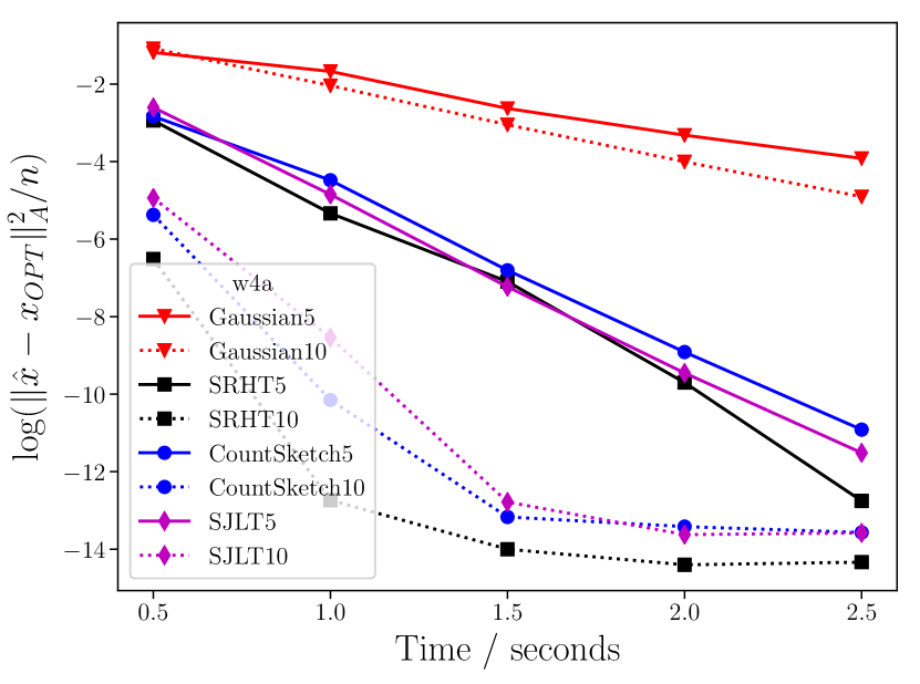
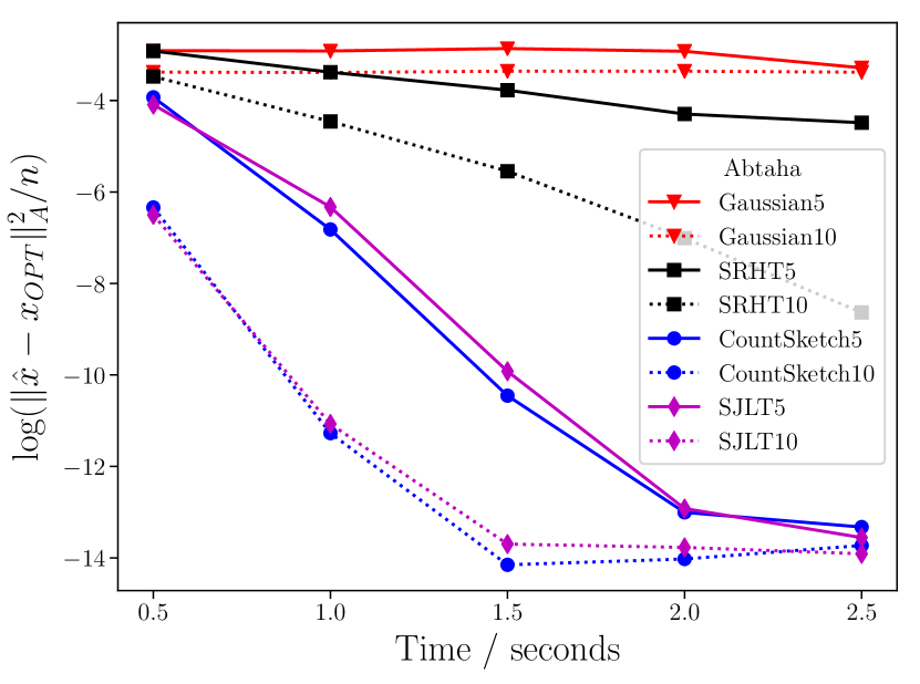
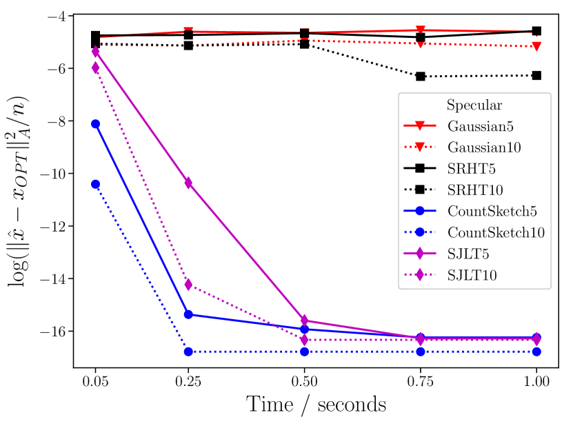
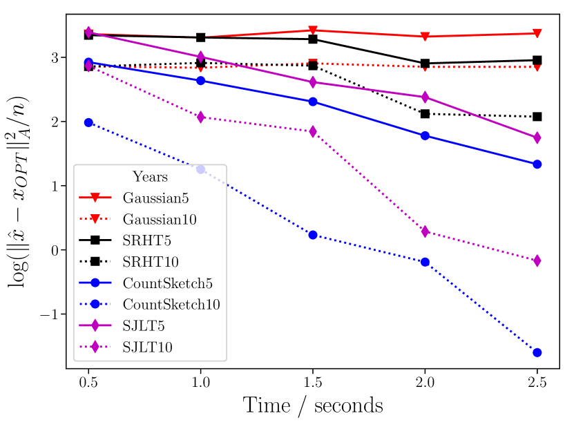
We study the empirical performance of our algorithms on instances of LASSO. In what follows, we write RP$(\gamma)$ to denote the random projection method RP with projection dimension $m=\gamma d$. For example, SRHT$({10})$ is an SRHT projection with projection dimension $m=10d$. Details of the datasets we test can be found in Appendix B. Also given in Appendix B is an example of the baseline experiments which justify the observed performance of, in particular, the CountSketch. For the fairest comparison with SRHT we take 10 independent trials with $2^{\lfloor\log_{2}(n)\rfloor}$ samples chosen uniformly at random. In summary, for data with $n\gg d$, the CountSketch returns an embedding of comparable accuracy up to 100x faster than the dense methods on sparse data. At a fixed projection dimension, observing comparable accuracy with the CountSketch is unexpected given its theoretical dependence on $O(d^{2})$ for a subspace embedding.

Experimental Setup. We fix $\lambda=5.0$ and use this to define an instance of LASSO regression $x_{OPT}=\operatorname*{argmin}_{x\in\mathbb{R}^{d}}\frac{1}{2}\|Ax-b\|_{2}^{2}+\lambda\|x\|_{1}$. This choice of $\lambda$ ensures that all solutions $x_{OPT}$ are bounded away from zero so that the algorithm cannot report zero as a viable approximation. Each iteration builds a smaller quadratic program (in terms of $n$) which is solved exactly, akin to Gaines et al. (2018). We tested 10 independent runs of the algorithm and plot mean error against wall clock time. Our choice of projection dimension $m$ is guided by our theoretical analysis (which requires $\varepsilon<\frac{1}{2}$) and calibration experiments which suggest appropriate accuracy can be obtained when $m\geq 5d$. The SJLT was initialised with column sparsities $s=1$ and $s=4$ and we compare to SRHT and Gaussian transforms.

Results. Faster convergence is seen when sketch sizes are larger. Sparse sketches have only a mild increase in the summary time when the projection dimension $m$ is increased. Hence, one should aim to tradeoff with making the sketch as large as possible while not inhibiting the number of iterations that can be completed. For the smalllest sketch size $m=5d$, there is less difference between the competing methods. For larger sketches, CountSketch is much faster to reduce error, since we can perform more iterations in the same time. While sketch size has limited impact on iteration cost, larger sketches have lower error so descend to the optimum faster.

The w$n$a ($n=4,6,8$) are training sets of increasing size taken from a single dataset (Platt, 1998). When possible (w$4$a, w$6$a), the SRHT makes a small number of high quality iterations and has comparable performance to the sparse embeddings but as $n$ grows it becomes less competitive (as seen in all other examples). We see that more progress is made in fewer iterations using the SRHT (when this is possible). Even for the smallest instance, the cost of applying Gaussian random projections is prohibitively slow. In contrast, both the sparse methods with $m=10d$ achieve similar error to SRHT$({10})$. On w$6$a (Figure 1(b)) we see a marked improvement in the error behaviour of the sparse sketches at a projection dimension of $m=10d$. On the w$8$a dataset we see that using the SRHT becomes uncompetitive on large sparse datasets.

Large and sparse datasets. To see how the sketches perform as we encounter very large and sparse data we also repeat the experiment on the Specular dataset. Figure 1(e) shows that yet again the sparse embeddings dominate the dense projections in terms of error. Rapid convergence is seen with CountSketch$({10})$ which reaches machine precision and terminates in 0.25 seconds. Very similar behaviour is seen with CountSketch$({5})$ as almost all of the progress is made in 0.25 seconds. he SJLT$({10})$ performs similarly to CountSketch$({5})$ in terms of error decay. However, when $m=5d$ we begin to notice a slight deterioration in performance of the SJLT$({5})$ compared to CountSketch$({5})$ and CountSketch$({10})$: the marginally increased sketch time costs to generate the SJLT now begins to play a role as the CountSketches have complete more iterations in a given time and hence made further progress. Similarly, the SJLT$({5})$ incurs slightly higher per-iteration error than the SJLT$({10})$ so less progress is made in the allotted time. In spite of this, both CountSketch$({\cdot})$ and SJLT$({\cdot})$ perform significantly better than the dense methods for which the data is so large that operating on the dense arrays becomes infeasible.

Conclusion. We have shown the Iterative Hessian Sketch (IHS) framework can be used effectively for scenarios with large $n$, and $n\gg d$, using fast sparse embeddings. A consequence of this is much faster descent towards the optimal solution than the state of the art, on data both sparse and dense. CountSketch tends to be the overall fastest method to converge on a solution, despite having weaker theoretical guarantees. SJLT has to do more work per iteration to build the sketch, and so the saving in the number of iterations to converge is not quite enough to compensate. An interesting direction is to reduce the need for access to the data, and to aim for making just a single pass over the data.

Appendix A Technical Results

A.1 IHS with Sparse Embeddings

Throughout, we consider instances of overconstrained regression (1) given in the form of a data matrix $A\in\mathbb{R}^{n\times d}$, target vector $b\in\mathbb{R}^{n}$ with $n\gg d$ and convex constraints $\mathcal{C}$. Our aim is to provide solution approximation guarantees for this system as given in Definition A.1. Let $f(x)=\frac{1}{2}\|Ax-b\|_{2}^{2}$ for input parameters $(A,b)$ and let $x_{OPT}$ denote the optimal (constrained) solution of our instance. The IHS approach performs a sequence of sketching steps via (2) to approximate $x_{OPT}$.

Definition A.1.

An algorithm which returns $\hat{x}$ such that $\|x_{OPT}-\hat{x}\|_{A}\leq\varepsilon\|x_{OPT}\|_{A}$ is referred to as a $\varepsilon$-solution approximation algorithm, where $\|x\|_{A}=\frac{1}{\sqrt{n}}\|Ax\|_{2}$.

Time Costs. The time taken for each approach is similar, and is determined by the combination of the sketch time $T_{\text{sketch}}$ and the time to solve a smaller problem in the ‘sketch space’, $T_{\text{solve}}$. We typically project data to a $\tilde{O}(d)\times d$ size matrix, so $T_{\text{solve}}$ is $\tilde{O}(d^{3})$. For the IHS method, we typically require $O(\log 1/\varepsilon)$ iterations to reach convergence.

We next outline the technical arguments needed to use CountSketch and SJLT in IHS. We make use of the following result regarding subspace embeddings.

Theorem A.2 (Woodruff (2014)).

Let $A\in\mathbb{R}^{n\times d}$ have full column rank. Let $S\in\mathbb{R}^{m\times n}$ be sampled from one of the Gaussian, SRHT, or CountSketch distributions. Then to achieve the subspace embedding property with probability $1-\delta$ we require $m=O(\varepsilon^{-2}(d+\log(1/\delta)))$ for the Gaussian and SJLT sketches; $m=\Omega(\varepsilon^{-2}(\log d)(\sqrt{d}+\sqrt{n})^{2})$ for the SRHT; and $m=O(d^{2}/(\delta\varepsilon^{2}))$ for the CountSketch.

A.1.1 Instantiating the Iterative Hessian Sketch

First we need that the sketches are zero mean and have identity covariance $\mathbb{E}[S^{T}S]=I_{n}$ which is shown in Lemma A.7. Note that for SJLT with $s>1$ we need to normalise by the number of nonzeros to ensure identity covariance. Two further properties are required for the error bounds of the IHS. These are given in Equation (4). However, to define these properties, we first introduce Definition A.3, after which we can present the proof of Theorem 2.2.

Definition A.3.

The tangent cone is the following set:

$$K=\{v\in\mathbb{R}^{d}:v=tA(x-x_{OPT}),~{}t\geq 0,x\in\mathcal{C}\}$$ (3)

We note that the residual error vector for an approximation $\hat{x}$ belongs to this set as $u=A(\hat{x}-x_{OPT})$. Let $X=K\cap\mathcal{S}^{n-1}$ where $\mathcal{S}^{n-1}$ is the set of $n$-dimensional vectors which have unit Euclidean norm. The quantities we must analyze are:

$$Z_{1}=\inf_{u\in X}\|Su\|_{2}^{2}\quad\text{~{} and ~{}}\quad Z_{2}=\sup_{u\in X}|u^{T}S^{T}Sv-u^{T}v|.$$ (4)

Here, $v$ denotes a fixed unit-norm $n$-dimensional vector.

Proof of Theorem 2.2..

We focus separately on the cases when $S$ is an SJLT or a CountSketch. Observe that when $S$ is a subspace embedding for the column space of $A$, we have for $u\in K\subseteq\text{col}(A)$ that $\|Su\|_{2}^{2}=(1\pm\varepsilon)\|u\|_{2}^{2}=(1\pm\varepsilon)$. Therefore, $Z_{1}\geq 1-\varepsilon$. Recalling Theorem A.2, we see that this is achieved for the SJLT with $m=\tilde{O}(d\log d)$ provided the column sparsity $s$ is sufficiently greater than 1. In contrast, for $s=1$, CountSketch has $m=\tilde{O}(d^{2})$ (here, $\tilde{O}$ suppresses the dependency on $\varepsilon$).

Next we focus on achieving $Z_{2}\leq\varepsilon/2$ for both sketches. If $s=\Omega(1/\varepsilon)$ then the SJLT immediately satisfies (4) by virtue of being a JLT. Note that this matches the lower bound on the column sparsity as stated in Remark A.4. In light of the column sparsity lower bound, we appeal to a different argument in order to use CountSketch within the IHS.

We invoke the approximate matrix product with sketching matrices for when $S\in\mathbb{R}^{m\times n}$ is a subspace embedding for $\text{col}(A)$ (Theorem 13 of Woodruff (2014) restated from Kane and Nelson (2014)). Define the matrices $U,V\in\mathbb{R}^{n\times d}$ whose first rows are $u$ and $v$, respectively, followed by $n-1$ rows of zeros. Now apply the CountSketch $S$ to each of $U$ and $V$ which will be zero except on the first row. Hence, the product $U^{T}S^{T}SV$ contains $\langle Su,Sv\rangle$ at $(U^{T}S^{T}SV)_{1,1}$ and is otherwise zero; likewise $U^{T}V$ contains only $\langle u,v\rangle$ at $(U^{T}V)_{1,1}$. The approximate matrix product result gives $\|U^{T}S^{T}SV-U^{T}V\|_{F}\leq 3\varepsilon\|U\|_{F}\|V\|_{F}$ for $\varepsilon\in(0,1/2)$; from which desired property follows after rescaling $\varepsilon$ by a constant. The definitions of $U,V,u,v$ mean $\|U\|_{F}=1,\|V\|_{F}=1$ and hence the error difference $U^{T}S^{T}SV-U^{T}V$ has exactly one element at $(i,j)=(1,1)$. This is exactly $|u^{T}S^{T}Sv-u^{T}v|$ and hence $Z_{2}\leq\varepsilon$ after rescaling. Coupled with the fact that the rows of a CountSketch matrix $S$ are sub-Gaussian (Section A.2), we are now free to use the CountSketch within the IHS framework. ∎

Remark A.4.

A lower bound on the column sparsity, namely $s=\Omega(d/\varepsilon)$ nonzeros per column, is needed to achieve a Johnson-Lindenstrauss Transform (JLT) (Kane and Nelson, 2014). It was also shown that if $s=\Omega(1/\varepsilon)$ then an SJLT will return a JLT. Hence, if $S$ is an SJLT subspace embedding with $s$ large enough, then the requirement on $Z_{2}$ is immediately met. However, for $s=1$, the CountSketch does not in general provide a full JLT due to the $\Omega(d/\varepsilon)$ lower bound. This result prevents the CountSketch, which has only a single nonzero in every column, from being a JLT, unless the data satisfies some strict requirements (Ailon and Chazelle, 2006).

Iteration Time Costs. The iterations require computing a subspace embedding at every step. The time cost to do this with sparse embeddings is: $O(s\text{nnz}(A))$ for sketching $A$. Additionally we require (i) $O(md^{2})$ to compute the approximate Hessian and (ii) $O(\text{nnz}(A))$ for the inner product terms in order to construct the intermediate quadratic program as in Equation (2). Solving the QP takes $\text{poly}(d)=\tilde{O}(d^{3})$ when $m=\tilde{O}(d)$ for the SJLT (the $\tilde{O}$ suppresses small $\log$ factors). For CountSketch, $m=\tilde{O}(d^{2})$, we require $\text{poly}(d)=\tilde{O}(d^{4})$. Overall, this is $O(\text{nnz}(A)+d^{3})$ for SJLT and $O(\text{nnz}(A)+d^{4})$ for CountSketch.

To summarize, we have shown that every iteration of the IHS can be completed in time proportional to the number of nonzeros in the data. with some (small) additional overhead to solve the QP at that time. Although there is some (small) additional overhead to solve the QP which is larger for the CountSketch than the SJLT, in practice, this increased time cost is not observed on the datasets we test. In comparison to previous state of the art, the per-step time cost using the SRHT will be $O(nd\log d+d^{3})$ and $O(nd^{2}+d^{3})$ for the Gaussian random projection.

A.2 Subgaussianity of CountSketch

Lemma A.5.

Let $S$ be a CountSketch matrix. Let $N_{i}$ denote the number of nonzeros in row $S_{i}$. Then $SS^{T}$ is a diagonal matrix with $(SS^{T})_{ii}=N_{i}$ and hence distinct rows of $S$ are orthogonal.

Proof.

The entries of matrix $SS^{T}$ are given by the inner products between pairs of rows of $S$. Consequently, we consider the inner product $\langle S_{i},S_{j}\rangle$. By construction $S$ has exactly one non-zero entry in each column. Hence for distinct rows $i\neq j$, $\langle S_{i},S_{j}\rangle=0$. Meanwhile, the diagonal entries are given by $\|S_{i}\|_{2}^{2}=\sum_{j=1}^{n}S_{ij}^{2}$, i.e. we simply count the number of non-zero entries in row $S_{i}$, which is $N_{i}$. ∎

Lemma A.6.

$\mathbb{E}[SS^{T}]=\frac{n}{m}I_{m}$

Proof.

Continuing the previous analysis, we have that $(SS^{T})_{ij}=\langle S_{i},S_{j}\rangle$, the inner product between rows of $S$. Taking the expectation, $\mathbb{E}[S_{i}\cdot S_{j}]=\sum_{k=1}^{n}\mathbb{E}[S_{ik}S_{jk}]$. By Lemma A.5, we know that for $i\neq j$ then $\langle S_{i},S_{j}\rangle=0$ and hence $\mathbb{E}[S_{i}\cdot S_{j}]=0.$ Otherwise, $i=j$ and we have a sum of $n$ random entries. With probability $\frac{1}{m}$, $S^{2}_{ik}=1$, coming from the two events $S_{ik}=-1$ with probability $\frac{1}{2m}$, and $S_{ik}=1$, also with probability $\frac{1}{2m}$. Then by linearity of expectation we have $\mathbb{E}[S_{i}\cdot S_{i}]=\sum_{k=1}^{n}\mathbb{E}S_{ik}^{2}=n/m$. ∎

Lemma A.7.

The covariance matrix is an identity, $\mathbb{E}[S^{T}S]=I_{n\times n}$

Proof.

Observe that $\mathbb{E}[S^{T}S]_{ij}=\langle S^{T}_{i},S^{j}\rangle=\langle S^{i},S^{j}\rangle$ so now we consider dot products betwen columns of $S$. Recall that each column $S^{i}$ is a basis vector with unit norm. Hence for $i=j$, $\langle S^{i},S^{i}\rangle=1$. For $i\neq j$, the inner product is only non-zero if $S^{i}$ and $S^{j}$ have their non-zero entry in the same location, $k$. The inner-product is $1$ when $S_{ki}$ and $S_{kj}$ have the same sign, and $-1$ when they have opposite signs. The probability of these two cases are equal, so the result is zero in expectation. In summary then, $\mathbb{E}[S^{T}S]_{ij}=1$ if $i=j$ and 0 otherwise which is exactly the $n\times n$ identity matrix. ∎

Definition A.8 (Pilanci and Wainwright (2016)).

A zero-mean random vector $s\in\mathbb{R}^{n}$ is sub-Gaussian if for any $u\in\mathbb{R}^{n}$ we have $\forall\varepsilon>0,\mathbb{P}[\langle s,u\rangle\geq\varepsilon\|u\|_{2}]\leq\exp(-\varepsilon^{2}/2)$.

The definition of a subgaussian random vector associates the inner product of a random vector and a fixed vector to the definition of sub-Gaussian random variables in the usual sense.

Lemma A.9 (Rows of CountSketch are sub-Gaussian).

Let $S$ be an $m\times n$ random matrix sampled according to the CountSketch construction. Then any row $S_{i}$ of $S$ is 1-sub-Gaussian.

Proof.

Fix a row $S_{i}$ of $S$ and let $X=\langle S_{i},u\rangle$. If either $S_{i}$ or $u$ is a zero vector then the inequality in the sub-Gaussian definition is trivially met, so assume that this is not the case. We need Bernstein’s Inequality: when $X$ is a sum of $n$ random variables $X_{1},\ldots,X_{n}$ and $|X_{j}|\leq M$ for all $j$ then for any $t>0$

$$\mathbb{P}(X>t)\leq\exp\bigg{(}-\frac{t^{2}/2}{\sum_{j}\mathbb{E}X_{j}^{2}+Mt/3}\bigg{)}.$$ (5)

Now consider $X=\sum_{j=1}^{n}S_{ij}u_{j}$, which is a sum of zero-mean random variables. We have $|X_{j}|=|S_{ij}u_{j}|\leq\|u\|_{2}$ for every $j$ and $\mathbb{E}X_{j}^{2}=u_{j}^{2}/m$. Taking $t=\varepsilon\|u\|_{2}$ in Equation (5) and cancelling $\|u\|_{2}^{2}$ terms gives $\mathbb{P}(X>\varepsilon\|u\|_{2})\leq\exp\left(-\frac{\varepsilon^{2}/2}{1/m+\varepsilon/3}\right)$. The RHS is at most $\exp(-\varepsilon^{2}/2)$ whenever $1/m+\varepsilon/3\leq 1$, which bounds $\varepsilon\leq 3-3/m$. Imposing $m>1$, this is satisfied for all $\varepsilon\in(0,1)$. ∎

Appendix B Data and Baselines

Table 1: Summary of datasets.

Dataset	Size $(n,d)$	Density	Source
Abtaha	$(37932,330)$	1%	Davis and Hu (2011)
Specular	$(477976,50)$	1%	Vanschoren et al. (2013)
W4A	$(7366,300)$	4%	Platt (1999)
W6A	$(17188,300)$	4%	Platt (1999)
W8A	$(49749,300)$	4%	Platt (1999)
YearPredictionsMSD	$(515344,90)$	100%	Dheeru and Karra Taniskidou (2017)

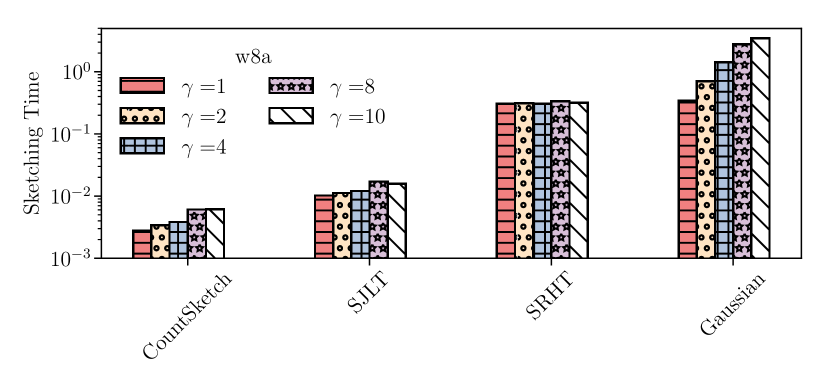
The properties of the datasets used for experiments is shown in Table 1. Figure 2 shows the mean empirical sketch error $\|A^{T}S^{T}SA-A^{T}A\|_{F}/\|A^{T}A\|_{F}$, and the sketch time baseline over ten independent trials on the w8a dataset. Similar performance is observed on the other datasets listed in Table 1.

(a) Empirical Sketching Error for w8a dataset

(b) Sketching time

Figure 2: Empirical measurements for w8a dataset ( Legend refers to both plots)

References

- (1)
- Ailon and Chazelle (2006) Nir Ailon and Bernard Chazelle. 2006. Approximate nearest neighbors and the fast Johnson-Lindenstrauss transform. In Proceedings of the thirty-eighth annual ACM symposium on Theory of computing. ACM, 557–563.
- Davis and Hu (2011) Timothy A Davis and Yifan Hu. 2011. The University of Florida sparse matrix collection. ACM Transactions on Mathematical Software (TOMS) 38, 1 (2011), 1.
- Dheeru and Karra Taniskidou (2017) Dua Dheeru and Efi Karra Taniskidou. 2017. UCI Machine Learning Repository. http://archive.ics.uci.edu/ml.
- Gaines et al. (2018) Brian R Gaines, Juhyun Kim, and Hua Zhou. 2018. Algorithms for fitting the constrained lasso. Journal of Computational and Graphical Statistics just-accepted (2018).
- Kane and Nelson (2014) Daniel M Kane and Jelani Nelson. 2014. Sparser johnson-lindenstrauss transforms. Journal of the ACM (JACM) 61, 1 (2014), 4.
- Pilanci and Wainwright (2016) Mert Pilanci and Martin J. Wainwright. 2016. Iterative Hessian sketch: Fast and Accurate solution approximation for constrained least-squares. The Journal of Machine Learning Research 17, 1 (2016), 1842–1879.
- Pilanci and Wainwright (2017) Mert Pilanci and Martin J Wainwright. 2017. Newton sketch: A near linear-time optimization algorithm with linear-quadratic convergence. SIAM Journal on Optimization 27, 1 (2017), 205–245.
- Platt (1998) John Platt. 1998. Sequential minimal optimization: A fast algorithm for training support vector machines. (1998).
- Platt (1999) John C Platt. 1999. 12 fast training of support vector machines using sequential minimal optimization. Advances in kernel methods (1999), 185–208.
- Vanschoren et al. (2013) Joaquin Vanschoren, Jan N. van Rijn, Bernd Bischl, and Luis Torgo. 2013. OpenML: Networked Science in Machine Learning. SIGKDD Explorations 15, 2 (2013), 49–60. https://doi.org/10.1145/2641190.2641198
- Woodruff (2014) David P. Woodruff. 2014. Sketching as a tool for numerical linear algebra. Foundations and Trends® in Theoretical Computer Science 10, 1–2 (2014), 1–157.