FutureMapping 2: Gaussian Belief Propagation for Spatial AI

Abstract

We argue the case for Gaussian Belief Propagation (GBP) as a strong algorithmic framework for the distributed, generic and incremental probabilistic estimation we need in Spatial AI as we aim at high performance smart robots and devices which operate within the constraints of real products. Processor hardware is changing rapidly, and GBP has the right character to take advantage of highly distributed processing and storage while estimating global quantities, as well as great flexibility. We present a detailed tutorial on GBP, relating it to the standard factor graph formulation used in robotics and computer vision, and give several simulation examples with code which demonstrate its properties.

1 Introduction

Spatial AI is the real-time vision-driven capability that robots and other devices need to understand and interact intelligently with the spaces around them, while satisfying the constraints such as power usage, compactness, robustness and simplicity enforced by real products. Davison [12], set out the case that there are still orders of magnitude of improvement needed in efficient performance to deliver the capabilities needed for breakthrough products such as lightweight home robots or AR glasses. Prototype real-time scene understanding systems in academia such as SemanticFusion [25] require heavy computing resources while delivering a fraction of the capability needed. While there is much ongoing effort in industry to optimise and engineer such methods for embedded implementation, we believe that there are many fundamental changes needed still to cross this gap across algorithms, processors and sensors.

In this follow-on paper we present the case for Gaussian Belief Propagation (GBP) as a very strong algorithmic framework for the distributed, generic and incremental probabilistic estimation we need in Spatial AI.

GBP is a special case of general Loopy Belief Propagation, where an estimation problem represented by a factor graph can be solved in an iterative manner by computation at the nodes of the graph and purely local message passing between then. It is at heart a simple algorithm but can in our experience be subtle to understand. Alongside broader discussion, we therefore give a very detailed derivation of BP and GBP from first principles, and link it directly with the factor graph and non-linear optimisation methods and terminology commonly used in robotics and computer vision. We present some demo implementations for 1D and 2D SLAM-like problems, with open source Python code available for readers to experiment further.

GBP is not novel, and has even previously been tested in SLAM settings [33], but has not yet been seriously used in practical Spatial AI problems. We believe that recent advances in computing hardware in particular make this the right time to re-evaluate its properties.

1.1 Spatial AI and Computer Architecture

Spatial AI at its core is a problem of incremental estimation, where a persistent scene model, with static and dynamic elements, must be stored and updated continually using data from various sources. Some data will be a flow of geometric measurements from a metric sensor; other data could be labelling output from a neural network; and yet more could be prior information from assumptions made at the start of the mapping process or communicated later on, such as the calibration parameters of a robot’s drive system. All of this data must be combined consistently into the chosen scene representation, which could be complicated and heterogeneous, consisting of multiple geometric and semantic representations such as meshes, volumes, learned shape spaces, semantic label fields, or the estimated locations of parametric CAD objects.

Current prototype Spatial AI systems, attempting to process this heterogeneous flow of data into complicated persistent representations via various estimation techniques, often have severe performance bottlenecks due to limits in the capacities of computation load, data storage or data transfer. We think that there are two promising and parallel lines of attack to enable progress here. One is to focus on scene representation, and to find new parameterisations of world models which allow high quality scene models to be built and maintained much more efficiently. The CodeSLAM [6] and SceneCode [47] projects for instance are steps in this direction, using deep learning to find coded, compressed representations of geometry and semantic labels which can then be optimised to fuse multi-view data.

The other is to look towards the changing landscape in computing and sensing hardware. (We highly recommend the recent PhD thesis of Julien Martel for ambitious thinking about this whole area [23]). Computing hardware is at the beginning of a revolution, as we move away from reliance on processors and memory systems designed either for completely general purpose use (CPUs) or computer graphics (GPUs) towards an era where AI, and perhaps Spatial AI in particular, are significant enough applications to drive the development of custom computing hardware.

Fitting computer architecture to applications, in particular with the aim of reducing power usage while maintaining performance, certainly entails massive parallelism [40]; but also, fundamentally, intermingling data storage and computation to reduce the ‘bits $\times$ millimetres’ through which data is moved. GPUs are now one of the main workhorses of AI computation, and are certainly very good for certain tasks in computer vision, but we believe that the future of Spatial AI compute will require much more flexible storage and computation. This is particularly true due to the closed-loop, incremental nature of Spatial AI, where new data must be continually compared to and combined with stored models. In SemanticFusion, a GPU is used for tasks such as CNN label prediction and dense image alignment. In industry, many specialised chips and architectures are emerging to accelerate important computer vision algorithms such as feature detection and tracking or even a whole visual odometry pipeline, and certainly there is a great deal of effort on developing specific architectures for CNNs. However, as examined in [12], a complete Spatial AI system requires many other computations, and current prototypes rely heavily on CPU work, main RAM storage, and high bandwidth data transfers.

New graph processors designs such as Graphcore’s IPU [1] are emerging which have taken quite general design choices towards enabling a different type of processing. The IPU is a massively parallel chip, but where the processing cores are embedded in a large amount of high performance on-chip memory which can be used generally for local storage and inter-core communication. In the IPU, computation works best when the storage it needs can be distributed around the chip close to the cores and there is no need ever to communicate with external off-chip memory. However, the total on-chip memory is relatively small compared to off-chip RAM so algorithmic choices to ‘recompute instead of store’ are advantageous.

Thinking even more generally, we can predict a future where many intelligent devices operate in a coordinated way within a space, some of them quite simple, and where efficiency in each device emphasizes local computation (‘edge compute’) and minimal inter-device communication. If these devices are to coordinate to estimate global quantities, the computation must also be graph-based and distributed, with local computation and storage.

1.2 Probabilistic Estimation on Factor Graphs

So we have a strong feeling that algorithms which can operate with purely local computation and in-place data storage on a graph, and communicate via message passing, will fit well with coming computer hardware. Let us consider the computation involved in Spatial AI in more detail. As laid out in [12], Spatial AI problems inherently involve various graphs, and that paper made suggestions about the rough way in which the storage and computation could be jointly arranged. The key point, however, is that in Spatial AI there are various structured sources of uncertain information (priors, cameras, other sensors) from which, in real-time, we must extract estimates of quantities (robot locations, map geometry, map labels, etc.) which are represented by variables which also have their own structure.

The fundamental theory for consistent fusion of many uncertain sources of data is Bayesian probability theory [18]. A very powerful and general representation of the probabilistic structure of inference problems is the factor graph. A factor graph is an undirected bipartite graph whose nodes are either variables or factors. The variables are numerical parameters of a system whose values we wish to estimate, but are not directly observable. The factors which join these variables represent constraints imposed by measurements from sensors or other information about the system (such as priors) which we are directly able to access.

Each factor is connected to the subset of variables it depends on, and specifies the probabilistic dependence of the observed measurement on the values of those variables. A variable is denoted $x_{i}$, and a factor is denoted $f_{s}$. The subset of variables which is connected to a particular factor $f_{s}$ is denoted ${{\mathbf{x}}}_{s}$. The interpretation is that $f_{s}({{\mathbf{x}}}_{s})=p(z_{s}|{{\mathbf{x}}}_{s})$ is the probability of the numerical measurement $z_{s}$ captured at node $s$ given the variables ${{\mathbf{x}}}_{s}$.

The bipartite connection pattern of a factor graph defines the factorisability structure of the whole probabilistic model, in that all factors $f_{s}$ are independent of each other. The vector of all variables is ${{\mathbf{x}}}=(x_{1},x_{2},\ldots)^{\top}$, and therefore the total joint probability distribution over all variables is the product of all factors:

$$p({{\mathbf{x}}})=\prod_{s}f_{s}({{\mathbf{x}}}_{s})~{}.$$ (1)

Interesting estimation problems in computer vision and robotics can invariably be analysed to determine their factor graph structure, and Dellaert and colleagues in particular [13] have played a very important role in increasing understanding of the power of the factor graph formulation in our field.

Now, as we will see, since each factor is a function of some subset of the variables, this joint distribution is some tangled function of all of the variables involved in the graph. Our goal in inference is to separate out one or more more variables of interest (or all of them) and determine their marginal probability distributions: individual probabilistic estimates which take all of the measurement information in the factors into account. The tangled form of the product which is the full joint distribution means that this is usually a computationally challenging problem.

The factor graph describing a Spatial AI problem may be very large and complicated, and will continuously change due to live, asynchronous measurements. Practical inference methods therefore often make various approximations, for instance by ignoring some measurements or priors, or ‘baking in’ certain aspects. For instance, in SemanticFusion (based on ElasticFusion [45]), the 3D reconstruction component runs by decoupling camera tracking and map updates into independent, alternating estimation processes, with only an occasional explicit loop closure optimisation to take account of camera drift in an approximate way. Further, the semantic labelling carried out is not used to improve the geometric estimation in any way, though this would make a lot of sense (to apply map smoothing to regions confidently labelled as floor or walls for instance).

We know how to represent the ideal joint estimation problem to take account of these measurements properly in a factor graph, but it has not been feasible to do inference on such complicated graphs in real-time in practical systems, due not only to to computational complexity but also system design complexity. Again, approximate things could be done such as pre-smoothing depth maps in response to semantic labelling before fusing them into the 3D model, but this risks dangerous ‘double counting’ of information, which is known to lead to over-confident Bayesian estimates. The effect of a particular prior or measurement should only appear once in the whole graph.

The purest representation of the knowledge in a Spatial AI problem is the factor graph itself, rather than probability distributions derived from it, which will always have to be stored with some approximation. What we are really seeking is an algorithm which implements Spatial AI in a distributed way on a computational resource like a graph processor, by storing the factor graph as the master representation and operating on it in place using local computation and message passing to implement estimation of variables as needed but taking account of global influence. We imagine messages continually bubbling around a large factor graph, which is changing continually with the addition of new measurement factors and variable nodes, and perhaps never reaching full convergence, but always being close in a way which can be controlled. It may be that estimation processes will proceed in an attention-driven way, using a lot of computation to bring high quality to currently important areas or aspects, which then are allowed to fade to a less up-to-date state once attention moves on, in a ‘just-in-time’ style [43].

We will return to these general ideas in later discussion, but let us first get more concrete still about probabilistic estimation techniques.

1.3 Distributable Estimation using Gaussian Distributions

Almost all serious, scalable probabilistic estimation is based on the core assumption of Gaussianity in ‘most’ measurement distributions and ‘most’ posterior variable distrubutions, ‘most’ of the time. We say this with full knowledge that many other representations of distributions have been used, from sampling to other explicit functional parameterisations. But again and again, we come back to Gaussians due to their fundamental properties of fitting real-world statistical processes and the efficient representation of high-dimensional distributions they allow as the ‘central’ distribution of probability theory [18].

The most important techniques in current geometric Spatial AI estimation are all Gaussian-based techniques such as Extended Kalman Filtering and Bundle Adjustment. Gaussian-based methods have very close links to linear algebra, because optimising Gaussian likelihoods is equivalent to least-squares minimisation which involves the solution of linear systems. When we write down the joint probability distribution (Equation 1) represented by a Gaussian factor graph, the result is a product of Gaussians. Finding the most probable variable values is equivalent to minimising the negative log of this probability distribution, which is a sum of terms which are quadratic functions of the variables. To find the minimum of this sum, we find the information matrix which depends of the Jacobians of the measurement functions with respect to the variables and the precision matrices of the measurements, and then must solve a linear system involving this information matrix. (This is done iteratively if the Gaussian measurement fuctions are non-linear in the variables.)

The key to the efficiency of this whole procedure is the form of the information matrix (which has the same sparsity structure as ${{\mathtt{J}}}^{\top}{{\mathtt{J}}}$, often discussed in optimisation problems, as long as measurement precision matrices are diagonal), which must be inverted to solve the linear system. Many decades of work have been devoted to studying the structure of this matrix and efficient algorithms for inverting it. In Spatial AI, extra interest and difficulty is due to the fact that the estimation problem in question is incremental, with estimates needed in real-time and measurements continually arriving. There has been much analysis of the trade-offs between filtering approaches which marginalise out old variables such as historic robot pose estimates and others which repeatedly solve a whole estimation problem from scratch [38].

Inverting large sparse information matrices has been tackled with a variety of classic methods which take advantage of sparsity patterns or some degree of parallelisation, such as Cholesky decomposition, Conjugate gradients, Jacobi, Gauss-Seidel, Red-Black ordering, Multigrid, etc. Good recent discussion of different optimisation methods in the context of robot vision was given by PhD theses by Zienkiewicz [48], Engel [15] or Newcombe [27]. Particular sub-problems in Spatial AI have well-known information matrix structure. For instance, bundle adjustment for consistent scene reconstruction, where a relatively small number of cameras observe a large number of 3D points, has a factor graph where every factor joins one pose variable to one point variable, and on a CPU is well tackled using Cholesky decomposition [41], or on a GPU by the conjugate gradient method [46]. Surface reconstruction on a regular grid, where measurements from a sensor are combined with smoothness priors, can be parallelised with methods like the Primal Dual algorithm [8] Pure visual-inertial odometry can be tackled well with sliding window filtering or non-linear optimisation [26, 21].

However, as discussed earlier, prototype general Spatial AI systems need to have all of these elements and much more, and highly-tuned specific estimation modules have often been thrown together in unsatisfactory ways, requiring a lot of approximation of probabilistic structure or heavy computing resources, in particular with large data flows in and out of CPU RAM. General, efficient and scalable Spatial AI estimation needs to cope with various different dynamic factor graph patterns, involving priors and many types of measurements flowing into the graph. We need computation, storage and data transfer characteristics well matched to both the modules and their interfaces, and allowing practical incremental estimation.

Approaches such as iSAM2 from Kaess et al. [19] stand out as progress on taking a flexible approach to scalable incremental estimation. iSAM2, a CPU algorithm, uses a dynamic data structure called the Bayes Tree to represent a good approximation to the full factor graph of SLAM problems in such as way that most updates can be carried out with local message passing, with a more substantial editing operation needed only in response to rarer events such as loop closure.

We share the idea with iSAM2 of a factor graph as the master representation, but with graph computing hardware in mind we believe that we should be even more flexible. If we wish estimation on factor graphs to have the properties of purely local computation and data storage, we must get away from the idea that a ‘god’s eye view’ of the whole structure of the graph will ever be available. We are guided towards methods where each node of a processing and storage graph can operate with minimum knowledge of the whole graph structure — at a minimum, only purely local information about itself and its near neighbours.

This is the character of belief propagation, which in its purest form allows in-place inference on a factor graph with entirely local storage and processing. Each variable and factor node processes messages with no knowledge about the rest of the graph other than its direct neighbours, and BP can converge with arbitrary, asynchronous message passing schedules which need no global coordination. In a certain sense, an algorithm which works like this represents ‘assuming the worst’ — that no knowledge of the structure of an estimation problem is available to enable intelligent design of processing.

This is the reason both that BP is well worth studying as an end point in a continuum of possible methods, but also that it is unlikely to form the whole solution to practical estimation. What we foresee is that BP could form a general estimation ‘glue’ between specifically engineered hardware/software modules for particular tasks; or be particularly valuable in highly dynamic, rapidly reconfiguring estimation problems where management of computation can carry on in a decentralised way.

We will show that Gaussian Belief Propagation is a general tool which can be formulated for any standard problem that can be formulated as a factor graph, and can for instance handle non-linear measurement models and robust kernels.

Gaussian Belief Propagation has an extensive literature, and we are not the first to consider applying it to vision, robotics and SLAM problems, although we believe that it has received much less interest than it deserves in this context. Non-Gaussian Belief Propagation is much better known as a technique in computer vision for image processing tasks on regular image grids. Weiss and Freeman [44] did important work showing the generality and correctness of loopy GBP in an AI context.

Most relevant to us, Ranganathan et al. in their ‘Loopy SAM’ paper [33] showed GBP used for a robot mapping application, and their experiments have many similarities with the demonstrations we will give later in this paper. We believe that despite the promising results in that paper, there was not much follow-up due to the fact that the majority of researchers have been concentrating on CPU performance. Going back further, Paskin et al. [31] built a junction tree of a filtered SLAM graph which was kept sparse by removing edges and used GBP for inference. Work on Gaussian Processes in loopy graphs such by Sudderth et al. [39] is also related. More recently, Crandall et al. [10] used discrete BP to provide an initialisation for bundle adjustment, but then standard optimisation afterwards.

A more general research area which is strongly related is Multi-Robot SLAM [34, 9], where many approaches to distributed mapping have been studied over the years, though usually not with the granularity of distribution that we are currently considering and often focusing on the assembly and sharing of a few discrete maps.

2 Tutorial on Belief Propagation

We will first introduce the general theory of Belief Propagation, focusing on the Sum-Product Algorithm due to Pearl [32], and following the notation and derivation given in Bishop’s book ‘Pattern Recognition and Machine Learning’ [5] (note that this excellent book has now been made available as a free download). Here the representation of probability distributions is not specified, and could be discrete probability tables or otherwise. We will go on to derive the specific Gaussian case in Section 3, and readers already familiar with BP could skip straight to that section. We give a lot of detail on the mathematical derivations in these sections, with the aim of making them fully understandable for the committed reader.

We start from Equation 1 which defines the probability distribution over all variables in a factor graph as a product of all factors, and remember that in inference we aim to determine the marginal distribution over variables of interest. Choosing to start with one particular variable $x$, its marginal distribution is found by taking the joint distribution, and summing over all of the other variables:

$$p(x)=\sum_{{{\mathbf{x}}}\setminus x}p({{\mathbf{x}}})~{},$$ (2)

where the notation ${{\mathbf{x}}}\setminus x$ means all elements of ${{\mathbf{x}}}$ except $x$.

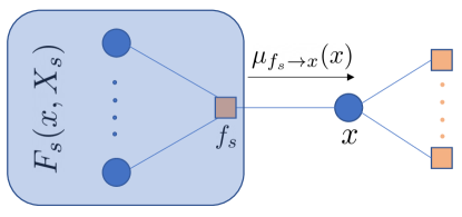
Figure 1: A variable node $x$ connects to factor nodes including $f_{s}$, from which it receives message $\mu_{f_{s}\rightarrow x}(x)$.

 

For the moment, we will assume that our factor graph has a tree structure, which means that it has no loops, and that there is precisely one route through the graph between any two nodes.

Consider Figure 1 which focuses on an arbitrary variable $x$ within a tree factor graph. Variable $x$ is directly connected to a number of factors $f_{s}$. Every other factor in the graph is connected to $x$ indirectly via exactly one of these factors, so we can divide the whole graph into the same number of subsets as the factors $f_{s}$, and write the whole joint probability distribution as a product of these subsets:

$$p({{\mathbf{x}}})=\prod_{s\in n(x)}F_{s}(x,{{\mathbf{X}}}_{s})~{}.$$ (3)

Here $n(x)$ is the set of factor nodes that are neighbours of $x$; $F_{s}$ is the product of all factors in the group associated with $f_{s}$; and ${{\mathbf{X}}}_{s}$ is the vector of all variables in the subtree connected to $x$ via $f_{s}$. Now, combining Equations 2 and 3:

$$p(x)=\sum_{{{\mathbf{x}}}\setminus x}\left[\prod_{s\in n(x)}F_{s}(x,{{\mathbf{X}}}_{s})\right]~{}.$$ (4)

We can reorder the sum and product to obtain:

$$p(x)=\prod_{s\in n(x)}\left[\sum_{{{\mathbf{X}}}_{s}}F_{s}(x,{{\mathbf{X}}}_{s})\right]~{}.$$ (5)

It is important to have a good intuition for what has happened with this switch. Each term $F_{s}(x,{{\mathbf{X}}}_{s})$ is the product of many factors; so it is a multivariate function of $x$ and all of the other variables in that branch of the tree. In Equation 4, we first multiply all of the $F_{s}$ terms together, to get a single joint function of all variables in the whole tree. In the sum, we then marginalise out over all other variables to be left with a marginal function only over our variable of interest $x$.

In Equation 5, on the other hand, we perform marginalisation first, taking each product of factors in a branch $F_{s}(x,{{\mathbf{X}}}_{s})$ and summing over all other variables to obtain a function only of $x$ in the square bracket for each branch. We then just calculate the product of these branch functions of $x$ to obtain the final marginal distribution over $x$.

We can start to see now the idea of using message passing terminology to describe this process. Continuing to use Bishop’s notation, we define:

$$\mu_{f_{s}\rightarrow x}(x)=\sum_{{{\mathbf{X}}}_{s}}F_{s}(x,{{\mathbf{X}}}_{s})~{}.$$ (6)

This term $\mu_{f_{s}\rightarrow x}(x)$ can be considered as a message from factor $f_{s}$ to variable $x$. The message has the form of a probability distribution over variable $x$ only, and is the marginalised probability over $x$ as the result of considering all factors in one branch of the tree: it is ‘what that branch of the tree says about the marginal probability distribution of $x$’. If variable $x$ receives such a message from all of the branches it is connected to, it can pool this information, and calculate its final marginal distribution by simply multiplying these messages together:

$$p(x)=\prod_{s\in n(x)}\mu_{f_{s}\rightarrow x}(x)~{}.$$ (7)

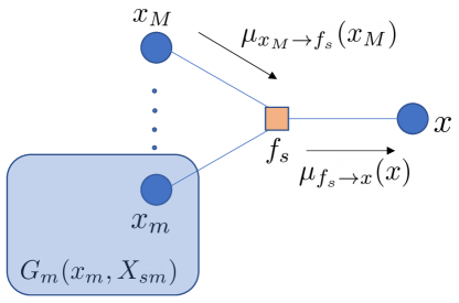
Figure 2: Factor $f_{s}$ connects variable $x$ to $M$ other neighbouring variables $x_{m}\in x_{1}\ldots x_{M}$, each of which is the root of a sub-branch containing a product of factors $G_{m}$.

 

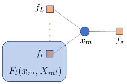
Figure 3: $x_{m}$, one of the variable neighbours of $f_{s}$, connects $f_{s}$ to the product of factors $G_{m}(x_{m},{{\mathbf{X}}}_{S_{m}})$ which we break down as $\prod_{l\in n(x_{m})\setminus f_{s}}F_{l}(x_{m},{{\mathbf{X}}}_{m_{l}})$.

 

Next, we go further into one of the branches of the tree, and break down the products of factors $F_{s}(x,{{\mathbf{X}}}_{s})$ as follows:

$$F_{s}(x,{{\mathbf{X}}}_{s}) = f_{s}(x,x_{1},\ldots,x_{M})$$

$$\times G_{1}(x_{1},{{\mathbf{X}}}_{S_{1}}),\ldots,G_{M}(x_{M},{{\mathbf{X}}}_{S_{M}})$$

$$= f_{s}(x,x_{1},\ldots,x_{M})\prod_{m\in n(f_{s})}G_{m}(x_{m},{{\mathbf{X}}}_{S_{m}})$$

Here, referring to Figure 2, $f_{s}$, the factor which connects $x$ to this branch, is a function of $x$ as well as $M$ other neighbouring variables $x_{m}\in x_{1}\ldots x_{M}$. Each of these variables connects to a sub-branch containing a product of factors $G_{m}$ which is a function of variable $x_{m}$ and other variables ${{\mathbf{X}}}_{S_{m}}$. Substituting into Equation 6:

$$\mu_{f_{s}\rightarrow x} (x)$$

$$= \sum_{{{\mathbf{X}}}_{s}}\left[f_{s}(x,x_{1},\ldots,x_{M})\prod_{m\in n(f_{s})}G_{m}(x_{m},{{\mathbf{X}}}_{S_{m}})\right]$$

$$= \sum_{x_{1},\ldots,x_{M}}\sum_{{{\mathbf{X}}}_{S_{1}},\ldots,{{\mathbf{X}}}_{S_{M}}}$$

$$\left[f_{s}(x,x_{1},\ldots,x_{M})\prod_{m\in n(f_{s})}G_{m}(x_{m},{{\mathbf{X}}}_{S_{m}})\right]$$

$$= \sum_{x_{1},\ldots,x_{M}}f_{s}(x,x_{1},\ldots,x_{M})$$ (13)

$$\prod_{m\in n(f_{s})}\sum_{{{\mathbf{X}}}_{S_{1}},\ldots,{{\mathbf{X}}}_{S_{M}}}G_{m}(x_{m},{{\mathbf{X}}}_{S_{m}})~{},$$

where we have made use of the fact that ${{\mathbf{X}}}_{s}=(x_{1},\ldots,x_{M},{{\mathbf{X}}}_{S_{1}},\ldots,{{\mathbf{X}}}_{S_{M}})$ to separate out the sum. We can now define the second type of message, this time from variable to factor:

$$\mu_{x_{m}\rightarrow f_{s}}(x_{m})=\sum_{{{\mathbf{X}}}_{s_{m}}}G_{m}(x_{m},{{\mathbf{X}}}_{S_{m}})~{},$$ (14)

and substitute into Equation 2 to get:

$$\mu_{f_{s}\rightarrow x}(x)=\sum_{x_{1},\ldots,x_{M}}f_{s}(x,x_{1},\ldots,x_{M})\prod_{m\in n(f_{s})}\mu_{x_{m}\rightarrow f_{s}}(x_{m})~{}.$$ (15)

We see here one half of the full recursive solution we are looking for: an expression for messages from factors to variables in terms of the messages those factors have received from other variables. We need just a few more steps to find ther other half of this. We need to take one more step deeper into the tree. Consider Figure 3, which now centres on $x_{m}$, one of the variable neighbours of $f_{s}$, which connects $f_{s}$ to the product of factors $G_{m}(x_{m},{{\mathbf{X}}}_{S_{m}})$. We break down this product as follows:

$$G_{m}(x_{m},{{\mathbf{X}}}_{S_{m}})=\prod_{l\in n(x_{m})\setminus f_{s}}F_{l}(x_{m},{{\mathbf{X}}}_{m_{l}})~{}.$$ (16)

We see that the total product factorises into terms $F_{l}(x_{m},{{\mathbf{X}}}_{m_{l}})$, each of which is the product of the set of factors from the whole graph which connects to $x_{m}$ via factor $f_{l}$. (We have broken down ${{\mathbf{X}}}_{S_{m}}$, the set of all variables connected to $f_{s}$ via $x_{m}$, into subsets ${{\mathbf{X}}}_{m_{l}}$ which connect to $x_{m}$ via factor $f_{l}$.)

We substitute this factorisation into Equation 14:

$$\mu_{x_{m}\rightarrow f_{s}}(x_{m})=\sum_{{{\mathbf{X}}}_{s_{m}}}\prod_{l\in n(x_{m})\setminus f_{s}}F_{l}(x_{m},{{\mathbf{X}}}_{m_{l}})~{},$$ (17)

and as we have seen before swap the order of the sum and product to obtain:

$$\mu_{x_{m}\rightarrow f_{s}}(x_{m})=\prod_{l\in n(x_{m})\setminus f_{s}}\sum_{{{\mathbf{X}}}_{m_{l}}}F_{l}(x_{m},{{\mathbf{X}}}_{m_{l}})~{}.$$ (18)

Here we recognise the form of a message from factor to variable as defined in Equation 6, and substitute to obtain:

$$\mu_{x_{m}\rightarrow f_{s}}(x_{m})=\prod_{l\in n(x_{m})\setminus f_{s}}\mu_{f_{l}\rightarrow x_{m}}(x_{m})~{}.$$ (19)

We now have all we need for the full sum-product algorithm, and can focus on Equations 7, 15 and 19. Equation 7 says that in order to calculate the marginal distribution for $x$, we should multiply together all of messages received from each of its neighbouring factor nodes. Each of those messages has the form of a probability distribution over $x$ only.

Stepping out to any one of the neighbouring factor nodes, we see the work that needs to be done at a factor node in Equation 15. A factor node receives messages from a number of variables, and must calculate a new message to send out. The messages that factor has received from other variables, each of which is a function of that one other variable, are all multiplied. We then multiply this product by the probability distribution representing the factor itself. We then marginalise out all variables other than the one to which the message will be sent, to leave a function of that variable only and that is the message that is sent.

One more step out, Equation 19 shows what happens at a variable node. It receives messages from a number of factors, all of which are functions of the variable, and multiplies these together to generate the message it sends on to the next factor.

It should now be clear that these two steps are simply repeated recursively through the whole tree. In order to find the marginal distribution for $x$, we start from all of the leaf nodes of the factor graph relative to $x$, which can be either variables or nodes, and pass messages inwards towards $x$. When each node has received messages from all outer nodes, it can perform its calculation to generate the correct message to pass inwards. This continues recursively all the way to $x$ at the root of the tree.

One remaining detail is how to initialise the leaf nodes, and this is simply dealt with. A variable leaf node sends a message $\mu_{x\rightarrow f}(x)=1$ to its only connected factor, and a factor leaf node sends $\mu_{f\rightarrow x}(x)=f(x)$. These are seen to be correct from looking at Equations 15 and 19 if we imagine a set of null factors with flat probability distributions surrounding the main tree.

So we know how to find the marginal distribution at a chosen node $x$ within a tree by defining that node as the root and passing messages recursively in towards it from all of the leaf nodes. If we required marginal distributions for all variable nodes in the tree, clearly we could simply repeat this procedure for each one. However, this would require a huge amount of wasted work. Imagine two variable nodes which are close together in a large tree. Defining either as the root node would lead to large equal branch and leaf structures in distant parts of the tree, and exactly the same computation in these regions would be repeated.

In fact, it is quite easy to see that we can find the marginal distribution for every variable node using only double the amount of work required to find the marginal for one variable. During the leaves-to-root message passing procedure to find the marginal for $x$, every variable and factor node along the way will have received incoming messages from all of its neighbours apart from the one to which it must transmit an outgoing message in the direction towards $x$. Once the messages get all the way the $x$, the root is then ‘fully informed’ and has a final marginal distribution which takes into account all of the measurement information in the graph. Therefore, if we now send a second series of messages outwards from the root back to the leaves, we will fill in the missing incoming message for every variable node and can therefore calculate a fully informed marginal for each one.

So belief propagation is able to efficiently determine marginal distributions for every variable in a tree graph with a one time forward/backward sweep of message passing through the graph. Most factor graphs for practical estimation problems are not trees however, but contain loops. This leads to two possibilities for the use of BP methods. One is to convert a general graph into a tree by combining nodes via graph cliques. These will be perfect trees, but with large compound nodes, and leads to the junction tree family of methods. The other is to retain the full loopy graph, but apply BP methods as if the graph was a tree, and keep iterating until convergence is reached. This approach is called loopy belief propagation, and has been shown to converge to useful solutions in many problems. We will test this out later, but first go on to derive the theory for belief propagation in the specific case that all probability distributions are Gaussian.

3 Gaussian Belief Propagation

In the case where the relationship between factors and variables is linear, and all factors have a Gaussian probability distribution, it is well understood that inference leads to a multivariate Gaussian distribution over the variables. It is also very well established that factor graphs which have factors which are Gaussians with non-linear dependence on the variables can be solved using efficient second order iterative optimisation (this is the class of non-linear least squares methods).

Here we will show how belief propagation can be implemented in this Gaussian case which is the norm in robotics and computer vision. Note that we have switched from scalars to vectors here for variable state space.

3.1 Factor Definition

We will start with a general specification of a factor which will be familiar to anyone used to probabilistic estimation in computer vision and robotics. Suppose that a robot has a sensor which is configured to observe a quantity which is a function of the state variables of the robot. When tested, the sensor is found to report measurements which differ from the expected ‘ground truth’ in a way described by a Gaussian distribution. We define the associated Gaussian factor as follows:

$$f_{s}({{\mathbf{x}}}_{s})=Ke^{-\frac{1}{2}\left[({{\mathbf{z}}}_{s}-{{\mathbf{h}}}_{s}({{\mathbf{x}}}_{s}))^{\top}{{\mathtt{\Lambda}}}_{s}({{\mathbf{z}}}_{s}-{{\mathbf{h}}}_{s}({{\mathbf{x}}}_{s}))\right]}~{}.$$ (20)

This expression represents the probability of obtaining vector measurement ${{\mathbf{z}}}_{s}$ from the sensor. Factor $f_{s}$ is a function of the set of involved variables ${{\mathbf{x}}}_{s}$, a subset of the whole state ${{\mathbf{x}}}$. The form of the function is a squared exponential with a scaling factor $K$ for normalisation whose value we will not need to calculate. Within the exponential, we see an inner product. This involves ${{\mathbf{h}}}_{s}$, the function which describes the dependence of the measurement on the variables, and ${{\mathbf{z}}}_{s}$, the value actually measured. Matrix ${{\mathtt{\Lambda}}}_{s}$ is the precision or inverse covariance of the measurement.

Note that we can also use factors of this form for priors which are not sensor measurements but assumptions or external knowledge, such as smoothness priors. We will look at the details of this in our examples later.

In summary, to specify a Gaussian factor, we need:

• ${{\mathbf{h}}}_{s}({{\mathbf{x}}}_{s})$, the functional form of the dependence of the measurement on the local state variables.

• ${{\mathbf{z}}}_{s}$, the actual observed value of the measurement.

• ${{\mathtt{\Lambda}}}_{s}$, the symmetric precision matrix of the measurement.

3.2 State Representation

In GBP, the probability distributions over state variables also have a Gaussian form. A Gaussian distribution in the state space of a particular variable node $m$ is generally written as:

$$p_{m}({{\mathbf{x}}}_{m})=Ke^{-\frac{1}{2}\left[({{\mathbf{x}}}_{m}-{{\boldsymbol{\mu}}}_{m})^{\top}{{\mathtt{\Lambda}}}_{m}({{\mathbf{x}}}_{m}-{{\boldsymbol{\mu}}}_{m})\right]}~{},$$ (21)

where ${{\boldsymbol{\mu}}}_{m}$ is the mean of the distribution and ${{\mathtt{\Lambda}}}_{m}$ is its precision or inverse covariance. An equivalent alternative form is:

$$p_{m}({{\mathbf{x}}}_{m})=K_{2}e^{\left[-\frac{1}{2}{{\mathbf{x}}}_{m}^{\top}{{\mathtt{\Lambda}}}_{m}{{\mathbf{x}}}_{m}+{{\boldsymbol{\eta}}}_{m}^{\top}{{\mathbf{x}}}_{m}\right]}~{}.$$ (22)

This is the information form, as explained very clearly for SLAM readers by Eustice et al. [16]. Note the different constant factor $K_{2}\neq K$, but we will not need to calculate the value of either. The information vector ${{\boldsymbol{\eta}}}_{m}$ is related to the mean vector by the relation:

$${{\boldsymbol{\eta}}}_{m}={{\mathtt{\Lambda}}}_{m}{{\boldsymbol{\mu}}}_{m}~{}.$$ (23)

From here on, we will represent a Gaussian distribution over vector ${{\mathbf{x}}}_{m}$ in this information form, using vector ${{\boldsymbol{\eta}}}_{m}$ and precision matrix ${{\mathtt{\Lambda}}}_{m}$. The information form is preferred to the covariance form as it can represent rank deficient Gaussian distributions with zero information which would correspond to an infinite covariance along dimensions which are fully unconstrained. The information form is also convenient as multiplication of distributions is handled simply by adding information vectors and precision matrices.

3.3 Linearising Factors

As in all types of scalable Gaussian-based estimation, we need to be able to produce a local linear version of any general non-linear factor in the form of Equation 20. Following Equations 21 and 22, a linear factor has the form of a Gaussian distribution over the variables ${{\mathbf{x}}}_{s}$ involved in the factor, expressed either in mean/precision form as:

$$f_{s}({{\mathbf{x}}}_{s})=Ke^{-\frac{1}{2}\left[({{\mathbf{x}}}_{s}-{{\boldsymbol{\mu}}}_{s})^{\top}{{\mathtt{\Lambda}}}_{s}^{\prime}({{\mathbf{x}}}_{s}-{{\boldsymbol{\mu}}}_{s})\right]}~{},$$ (24)

or information form:

$$f_{s}({{\mathbf{x}}}_{s})=K_{2}e^{\left[-\frac{1}{2}{{\mathbf{x}}}_{s}^{\top}{{\mathtt{\Lambda}}}_{s}^{\prime}{{\mathbf{x}}}_{s}+{{\boldsymbol{\eta}}}_{s}^{\top}{{\mathbf{x}}}_{s}\right]}~{}.$$ (25)

where mean ${{\boldsymbol{\mu}}}_{s}$, precision ${{\mathtt{\Lambda}}}_{s}^{\prime}$ and information vector ${{\boldsymbol{\eta}}}_{s}$ are related by:

$${{\boldsymbol{\eta}}}_{s}={{\mathtt{\Lambda}}}_{s}^{\prime}{{\boldsymbol{\mu}}}_{s}~{}.$$ (26)

Concentrating on the information form of Equation 25, we need to find the values of ${{\boldsymbol{\eta}}}_{s}$ and ${{\mathtt{\Lambda}}}_{s}^{\prime}$ to linearise the nonlinear constraint of Equation 20 around a state estimate ${{\mathbf{x}}}_{s}={{\mathbf{x}}}_{0}$. First, let us rewrite Equation 20 as:

$$f_{s}({{\mathbf{x}}}_{s})=Ke^{-\frac{1}{2}E_{s}}~{},$$ (27)

where $E_{s}$, the least squares ‘energy’ of the constraint, is:

$$E_{s}=({{\mathbf{z}}}_{s}-{{\mathbf{h}}}_{s}({{\mathbf{x}}}_{s}))^{\top}{{\mathtt{\Lambda}}}_{s}({{\mathbf{z}}}_{s}-{{\mathbf{h}}}_{s}({{\mathbf{x}}}_{s}))~{}.$$ (28)

Then we apply the first order Taylor series expansion of non-linear measurement function ${{\mathbf{h}}}_{s}$ to find its approximate value for state values ${{\mathbf{x}}}_{s}$ close to ${{\mathbf{x}}}_{0}$:

$${{\mathbf{h}}}_{s}({{\mathbf{x}}}_{s})\approx{{\mathbf{h}}}_{s}({{\mathbf{x}}}_{0})+{{\mathtt{J}}}_{s}({{\mathbf{x}}}_{s}-{{\mathbf{x}}}_{0})~{},$$ (29)

where ${{\mathtt{J}}}_{s}$ is the Jacobian $\frac{\partial{{\mathbf{h}}}_{s}}{\partial{{\mathbf{x}}}_{s}}\big{|}_{{{\mathbf{x}}}_{s}={{\mathbf{x}}}_{0}}$. Substituting into Equation 28 and rearranging:

$$E_{s} = \left[{{\mathbf{z}}}_{s}-({{\mathbf{h}}}_{s}({{\mathbf{x}}}_{0})+{{\mathtt{J}}}_{s}({{\mathbf{x}}}_{s}-{{\mathbf{x}}}_{0}))\right]^{\top}$$ (30)

$${{\mathtt{\Lambda}}}_{s}\left[{{\mathbf{z}}}_{s}-({{\mathbf{h}}}_{s}({{\mathbf{x}}}_{0})+{{\mathtt{J}}}_{s}({{\mathbf{x}}}_{s}-{{\mathbf{x}}}_{0}))\right]$$

$$= \left[({{\mathbf{z}}}_{s}-{{\mathbf{h}}}_{s}({{\mathbf{x}}}_{0}))-{{\mathtt{J}}}_{s}({{\mathbf{x}}}_{s}-{{\mathbf{x}}}_{0}))\right]^{\top}$$

$${{\mathtt{\Lambda}}}_{s}\left[({{\mathbf{z}}}_{s}-{{\mathbf{h}}}_{s}({{\mathbf{x}}}_{0}))-{{\mathtt{J}}}_{s}({{\mathbf{x}}}_{s}-{{\mathbf{x}}}_{0}))\right]$$

$$= ({{\mathbf{z}}}_{s}-{{\mathbf{h}}}_{s}({{\mathbf{x}}}_{0}))^{\top}{{\mathtt{\Lambda}}}_{s}({{\mathbf{z}}}_{s}-{{\mathbf{h}}}_{s}({{\mathbf{x}}}_{0}))$$

$$-({{\mathbf{z}}}_{s}-{{\mathbf{h}}}_{s}({{\mathbf{x}}}_{0}))^{\top}{{\mathtt{\Lambda}}}_{s}{{\mathtt{J}}}_{s}({{\mathbf{x}}}_{s}-{{\mathbf{x}}}_{0})$$

$$-({{\mathtt{J}}}_{s}({{\mathbf{x}}}_{s}-{{\mathbf{x}}}_{0}))^{\top}{{\mathtt{\Lambda}}}_{s}({{\mathbf{z}}}_{s}-{{\mathbf{h}}}_{s}({{\mathbf{x}}}_{0}))$$

$$+({{\mathtt{J}}}_{s}({{\mathbf{x}}}_{s}-{{\mathbf{x}}}_{0}))^{\top}{{\mathtt{\Lambda}}}_{s}{{\mathtt{J}}}_{s}({{\mathbf{x}}}_{s}-{{\mathbf{x}}}_{0})~{}.$$

The first of the four terms here is a constant which doesn’t depend on ${{\mathbf{x}}}_{s}$, and the second and third are equal (one is the transpose of the other, and both are scalars), so we can simplify to:

$$E_{s} = K_{3}-2({{\mathbf{z}}}_{s}-{{\mathbf{h}}}_{s}({{\mathbf{x}}}_{0}))^{\top}{{\mathtt{\Lambda}}}_{s}{{\mathtt{J}}}_{s}({{\mathbf{x}}}_{s}-{{\mathbf{x}}}_{0})$$

$$+({{\mathtt{J}}}_{s}({{\mathbf{x}}}_{s}-{{\mathbf{x}}}_{0}))^{\top}{{\mathtt{\Lambda}}}_{s}{{\mathtt{J}}}_{s}({{\mathbf{x}}}_{s}-{{\mathbf{x}}}_{0})$$

$$= ({{\mathbf{x}}}_{s}-{{\mathbf{x}}}_{0})^{\top}{{\mathtt{\Lambda}}}_{s}^{\prime}({{\mathbf{x}}}_{s}-{{\mathbf{x}}}_{0})$$

$$-2({{\mathbf{z}}}_{s}-{{\mathbf{h}}}_{s}({{\mathbf{x}}}_{0}))^{\top}{{\mathtt{\Lambda}}}_{s}{{\mathtt{J}}}_{s}({{\mathbf{x}}}_{s}-{{\mathbf{x}}}_{0})+K_{3}~{},$$

where ${{\mathtt{\Lambda}}}_{s}^{\prime}={{\mathtt{J}}}_{s}^{\top}{{\mathtt{\Lambda}}}_{s}{{\mathtt{J}}}_{s}$. Going further:

$$E_{s} = {{\mathbf{x}}}_{s}^{\top}{{\mathtt{\Lambda}}}_{s}^{\prime}{{\mathbf{x}}}_{s}-{{\mathbf{x}}}_{0}^{\top}{{\mathtt{\Lambda}}}_{s}^{\prime}{{\mathbf{x}}}_{s}-{{\mathbf{x}}}_{s}^{\top}{{\mathtt{\Lambda}}}_{s}^{\prime}{{\mathbf{x}}}_{0}+{{\mathbf{x}}}_{0}^{\top}{{\mathtt{\Lambda}}}_{s}^{\prime}{{\mathbf{x}}}_{0}$$ (31)

$$-2({{\mathbf{z}}}_{s}-{{\mathbf{h}}}_{s}({{\mathbf{x}}}_{0}))^{\top}{{\mathtt{\Lambda}}}_{s}{{\mathtt{J}}}_{s}{{\mathbf{x}}}_{s}$$

$$+2({{\mathbf{z}}}_{s}-{{\mathbf{h}}}_{s}({{\mathbf{x}}}_{0}))^{\top}{{\mathtt{\Lambda}}}_{s}{{\mathtt{J}}}_{s}{{\mathbf{x}}}_{0}+K_{3}~{}.$$

Here the second and third terms are equal, and the fourth and sixth are constant, so:

$$E_{s} = {{\mathbf{x}}}_{s}^{\top}{{\mathtt{\Lambda}}}_{s}^{\prime}{{\mathbf{x}}}_{s}-2{{\mathbf{x}}}_{0}^{\top}{{\mathtt{\Lambda}}}_{s}^{\prime}{{\mathbf{x}}}_{s}$$ (32)

$$-2({{\mathbf{z}}}_{s}-{{\mathbf{h}}}_{s}({{\mathbf{x}}}_{0}))^{\top}{{\mathtt{\Lambda}}}_{s}{{\mathtt{J}}}_{s}{{\mathbf{x}}}_{s}+K_{4}~{}.$$

From Equations 25 and 27 we see that the least squares energy in a linear constraint in the information form is:

$$E_{s}={{\mathbf{x}}}_{s}^{\top}{{\mathtt{\Lambda}}}_{s}^{\prime}{{\mathbf{x}}}_{s}-2{{\boldsymbol{\eta}}}_{s}^{\top}{{\mathbf{x}}}_{s}~{}.$$ (33)

Matching this with Equation 32:

$${{\boldsymbol{\eta}}}_{s}^{\top}={{\mathbf{x}}}_{0}^{\top}{{\mathtt{\Lambda}}}_{s}^{\prime}+({{\mathbf{z}}}_{s}-{{\mathbf{h}}}_{s}({{\mathbf{x}}}_{0}))^{\top}{{\mathtt{\Lambda}}}_{s}{{\mathtt{J}}}_{s}~{}.$$ (34)

And therefore, finally:

$${{\boldsymbol{\eta}}}_{s} = {{\mathtt{\Lambda}}}_{s}^{\prime}{{\mathbf{x}}}_{o}+{{\mathtt{J}}}_{s}^{\top}{{\mathtt{\Lambda}}}_{s}({{\mathbf{z}}}_{s}-{{\mathbf{h}}}_{s}({{\mathbf{x}}}_{0}))$$ (35)

$$= {{\mathtt{J}}}_{s}^{\top}{{\mathtt{\Lambda}}}_{s}\left[{{\mathtt{J}}}_{s}{{\mathbf{x}}}_{0}+{{\mathbf{z}}}_{s}-{{\mathbf{h}}}_{s}({{\mathbf{x}}}_{0})\right]~{}.$$

To summarise, to linearise a general non-linear factor ${{\mathbf{h}}}_{s}({{\mathbf{x}}}_{s})$ around state variables ${{\mathbf{x}}}_{0}$, turning it into a Gaussian factor expressed in terms of ${{\mathbf{x}}}_{s}$, we use the linear factor represented in information form by information vector ${{\boldsymbol{\eta}}}_{s}$ and precision matrix ${{\mathtt{\Lambda}}}_{s}^{\prime}$ calculated as follows:

$${{\boldsymbol{\eta}}}_{s} = {{\mathtt{J}}}_{s}^{\top}{{\mathtt{\Lambda}}}_{s}\left[{{\mathtt{J}}}_{s}{{\mathbf{x}}}_{0}+{{\mathbf{z}}}_{s}-{{\mathbf{h}}}_{s}({{\mathbf{x}}}_{0})\right]$$

$${{\mathtt{\Lambda}}}_{s}^{\prime} = {{\mathtt{J}}}_{s}^{\top}{{\mathtt{\Lambda}}}_{s}{{\mathtt{J}}}_{s}~{}.$$ (36)

3.4 Message Passing at a Variable Node

Let us now consider the computation which happens at nodes to implement message passing. Remember that in Belief Propagation, messages always have the form of a probability distribution in the state space of the variable node either sending or receiving the message. In GBP, each message will therefore take the form of an information vector and precision matrix in that state space.

First, we consider the processing that happens at a variable node ${{\mathbf{x}}}_{m}$ during message passing. A variable node is connected to a number of factors, and during a typical message passing step it receives incoming messages from all of these except one, and must generate an outgoing message to send to the remaining factor. Here we follow the recipe of Equation 19. All of the messages involved are in the state space of node ${{\mathbf{x}}}_{m}$. We simply need to multiply together all of the incoming messages to generate the outgoing message.

Each incoming message $\mu_{f_{l}\rightarrow{{\mathbf{x}}}_{m}}({{\mathbf{x}}}_{m})$ is represented by an information vector ${{\boldsymbol{\eta}}}_{ml}$ and a precision matrix ${{\mathtt{\Lambda}}}_{ml}$. We obtain the information vector and precision matrix of the outgoing message $\mu_{{{\mathbf{x}}}_{m}\rightarrow f_{s}}({{\mathbf{x}}}_{m})$ by simply adding:

$${{\boldsymbol{\eta}}}_{ms} = \sum_{l\in n({{\mathbf{x}}}_{m})\setminus f_{s}}{{\boldsymbol{\eta}}}_{ml}$$ (37)

$${{\mathtt{\Lambda}}}_{ms} = \sum_{l\in n({{\mathbf{x}}}_{m})\setminus f_{s}}{{\mathtt{\Lambda}}}_{ml}~{}.$$ (38)

This is because when we multiply several Gaussian expressions of the form in Equation 22, we add the exponents.

3.5 Message Passing at a Factor Node

A factor node receives incoming messages from a number of variable nodes, and must process these to produce an outgoing message to the target variable node. Following Equation 15, the incoming messages are multiplied together, and this product is also multiplied by the factor distribution itself. Now each of the incoming messages is a function of the state space of the variable node it comes from, while the factor potential is a function of all of the variables connected to the factor, including the output variable. The full product is therefore also a function of all variables. Finally, all variables other than the output variable are marginalised out from this joint distribution, and the result is a function only in the output variable’s state space, and this is the outgoing message.

The general non-linear factor ${{\mathbf{h}}}_{s}({{\mathbf{x}}}_{s})$ must be first linearised to an information vector ${{\boldsymbol{\eta}}}_{s}$ and precision matrix ${{\mathtt{\Lambda}}}_{s}^{\prime}$ as in Equation 36. This linearisation requires anchor values ${{\mathbf{x}}}_{0}$ of all of the connected variables, including the output variable. This can be done once every message passing step, or much less frequently. Clearly if a factor is a linear function in the first place then we formulate the linear constraint once and do not need to change it.

To the information vector and precision matrix representing the constraint, we add the incoming messages from input variables. This vector and matrix addition is done ‘in place’. In the vector of variables ${{\mathbf{x}}}_{s}$ associated with the factor, there should be a partitioning into contiguous sets which come from each connected variable node. E.g. let us consider a factor with three connected variable nodes, where $m_{1}$ $m_{2}$ are input nodes and $m_{3}$ is the output node in this case. In the factor definition:

$${{\mathbf{x}}}_{s}=\left(\begin{array}[]{c}{{\mathbf{x}}}_{sm_{1}}\\ {{\mathbf{x}}}_{sm_{2}}\\ {{\mathbf{x}}}_{sm_{3}}\end{array}\right)~{}.$$ (39)

The information vector and precision matrix are partitioned in the same way:

$${{\boldsymbol{\eta}}}_{s} = \left(\begin{array}[]{c}{{\boldsymbol{\eta}}}_{sm_{1}}\\ {{\boldsymbol{\eta}}}_{sm_{2}}\\ {{\boldsymbol{\eta}}}_{sm_{3}}\end{array}\right)$$ (43)

$${{\mathtt{\Lambda}}}_{s}^{\prime} = \left[\begin{array}[]{ccc}{{\mathtt{\Lambda}}}_{sm_{1}m_{1}}^{\prime}&{{\mathtt{\Lambda}}}_{sm_{1}m_{2}}^{\prime}&{{\mathtt{\Lambda}}}_{sm_{1}m_{3}}^{\prime}\\ {{\mathtt{\Lambda}}}_{sm_{2}m_{1}}^{\prime}&{{\mathtt{\Lambda}}}_{sm_{2}m_{2}}^{\prime}&{{\mathtt{\Lambda}}}_{sm_{2}m_{3}}^{\prime}\\ {{\mathtt{\Lambda}}}_{sm_{3}m_{1}}^{\prime}&{{\mathtt{\Lambda}}}_{sm_{3}m_{2}}^{\prime}&{{\mathtt{\Lambda}}}_{sm_{3}m_{3}}^{\prime}\end{array}\right]~{}.$$ (47)

So when conditioning on the messages coming from input notes $m_{1}$ and $m_{2}$ we get:

$${{\boldsymbol{\eta}}}_{Cs}=\left(\begin{array}[]{c}{{\boldsymbol{\eta}}}_{sm_{1}}+{{\boldsymbol{\eta}}}_{m_{1}s}\\ {{\boldsymbol{\eta}}}_{sm_{2}}+{{\boldsymbol{\eta}}}_{m_{2}s}\\ {{\boldsymbol{\eta}}}_{sm_{3}}\end{array}\right)\\$$ (48)

$${{\mathtt{\Lambda}}}_{Cs}^{\prime}=\left[\begin{array}[]{ccc}{{\mathtt{\Lambda}}}_{sm_{1}m_{1}}^{\prime}+{{\mathtt{\Lambda}}}_{m_{1}s}&{{\mathtt{\Lambda}}}_{sm_{1}m_{2}}^{\prime}&{{\mathtt{\Lambda}}}_{sm_{1}m_{3}}^{\prime}\\ {{\mathtt{\Lambda}}}_{sm_{2}m_{1}}^{\prime}&{{\mathtt{\Lambda}}}_{sm_{2}m_{2}}^{\prime}+{{\mathtt{\Lambda}}}_{m_{2}s}&{{\mathtt{\Lambda}}}_{sm_{2}m_{3}}^{\prime}\\ {{\mathtt{\Lambda}}}_{sm_{3}m_{1}}^{\prime}&{{\mathtt{\Lambda}}}_{sm_{3}m_{2}}^{\prime}&{{\mathtt{\Lambda}}}_{sm_{3}m_{3}}^{\prime}\end{array}\right]~{}.$$ (49)

To complete message passing, from this joint distribution we must marginalise out all variables but those of the output node, in this example $m_{3}$. Eustice et al. [16] give the formula for marginalising a general partioned Gaussian state in information form. If the joint distribution is:

$${{\boldsymbol{\eta}}} = \left(\begin{array}[]{c}{{\boldsymbol{\eta}}}_{\alpha}\\ {{\boldsymbol{\eta}}}_{\beta}\end{array}\right)$$ (52)

$${{\mathtt{\Lambda}}} = \left[\begin{array}[]{cc}{{\mathtt{\Lambda}}}_{\alpha\alpha}&{{\mathtt{\Lambda}}}_{\alpha\beta}\\ {{\mathtt{\Lambda}}}_{\beta\alpha}&{{\mathtt{\Lambda}}}_{\beta\beta}\end{array}\right]~{},$$ (55)

then marginalising out the $\beta$ variables to leave a distribution only over the $\alpha$ set is achieved by:

$${{\boldsymbol{\eta}}}_{M\alpha} = {{\boldsymbol{\eta}}}_{\alpha}-{{\mathtt{\Lambda}}}_{\alpha\beta}{{\mathtt{\Lambda}}}_{\beta\beta}^{-1}{{\boldsymbol{\eta}}}_{\beta}$$ (56)

$${{\mathtt{\Lambda}}}_{M\alpha} = {{\mathtt{\Lambda}}}_{\alpha\alpha}-{{\mathtt{\Lambda}}}_{\alpha\beta}{{\mathtt{\Lambda}}}_{\beta\beta}^{-1}{{\mathtt{\Lambda}}}_{\beta\alpha}~{}.$$ (57)

To apply these formulae to the partitioned state of Equations 48 and 49, we first reorder the vector and matrix to bring the output variable to the top. For our example where $m_{3}$ is the output variable, we reorder the conditioned vector and matrix:

$${{\boldsymbol{\eta}}}_{Cs} = \left(\begin{array}[]{c}{{\boldsymbol{\eta}}}_{{Cs}m_{1}}\\ {{\boldsymbol{\eta}}}_{{Cs}m_{2}}\\ {{\boldsymbol{\eta}}}_{{Cs}m_{3}}\end{array}\right)$$ (61)

$${{\mathtt{\Lambda}}}_{Cs}^{\prime} = \left[\begin{array}[]{ccc}{{\mathtt{\Lambda}}}_{{Cs}m_{1}m_{1}}^{\prime}&{{\mathtt{\Lambda}}}_{{Cs}m_{1}m_{2}}^{\prime}&{{\mathtt{\Lambda}}}_{{Cs}m_{1}m_{3}}^{\prime}\\ {{\mathtt{\Lambda}}}_{{Cs}m_{2}m_{1}}^{\prime}&{{\mathtt{\Lambda}}}_{{Cs}m_{2}m_{2}}^{\prime}&{{\mathtt{\Lambda}}}_{{Cs}m_{2}m_{3}}^{\prime}\\ {{\mathtt{\Lambda}}}_{{Cs}m_{3}m_{1}}^{\prime}&{{\mathtt{\Lambda}}}_{{Cs}m_{3}m_{2}}^{\prime}&{{\mathtt{\Lambda}}}_{{Cs}m_{3}m_{3}}^{\prime}\end{array}\right]$$ (65)

to:

$${{\boldsymbol{\eta}}}_{CRs} = \left(\begin{array}[]{c}{{\boldsymbol{\eta}}}_{{Cs}m_{3}}\\ {{\boldsymbol{\eta}}}_{{Cs}m_{1}}\\ {{\boldsymbol{\eta}}}_{{Cs}m_{2}}\end{array}\right)$$ (69)

$${{\mathtt{\Lambda}}}_{CRs}^{\prime} = \left[\begin{array}[]{ccc}{{\mathtt{\Lambda}}}_{{Cs}m_{3}m_{3}}^{\prime}&{{\mathtt{\Lambda}}}_{{Cs}m_{3}m_{1}}^{\prime}&{{\mathtt{\Lambda}}}_{{Cs}m_{3}m_{2}}^{\prime}\\ {{\mathtt{\Lambda}}}_{{Cs}m_{1}m_{3}}^{\prime}&{{\mathtt{\Lambda}}}_{{Cs}m_{1}m_{1}}^{\prime}&{{\mathtt{\Lambda}}}_{{Cs}m_{1}m_{2}}^{\prime}\\ {{\mathtt{\Lambda}}}_{{Cs}m_{2}m_{3}}^{\prime}&{{\mathtt{\Lambda}}}_{{Cs}m_{2}m_{1}}^{\prime}&{{\mathtt{\Lambda}}}_{{Cs}m_{2}m_{2}}^{\prime}\end{array}\right]$$ (73)

We then identify subblocks $\alpha=m_{3}$ and $\beta=m_{1}m_{2}$ between Equations 52, 55 and Equations 69, 73, and apply Equations 56 and 57 to obtain the marginalised distribution over $m_{3}$ which forms the outgoing message $\mu_{f_{s}\rightarrow{{\mathbf{x}}}_{m_{3}}}$ to variable node $m_{3}$.

3.6 Implemention Details

One of the great strengths of GBP is the straightforward and fully local nature of implementation. We believe that whereas previous estimation methods are instantiated in large and highly optimised ‘solver’ libraries for a CPU, the details of GBP can be easily and efficiently implemented on any particular distributed platform, and what is more likely to emerge is a set of standard formats for how these platforms should pass messages between them, befitting our prediction of great value for GBP as the glue between other estimation methods.

Our current simple CPU implementation is a prototype for future implementation on a graph processor or other distributed device, and therefore has decentralisation of data and processing into classes. A VariableNode or FactorNode class object is instantiated for each node of the factor graph. Specialisations of these implement the particular state space and factor function models of the graph in question, and the algorithms for message passing. However, these classes do not store any state information. An Edge object is instantiated for every connection between a variable and a factor, and stores the latest VariableToFactorMessage and FactorToVariableMessage for this link. So when a VariableNode or FactorNode needs to carry out a message passing step, it reads the appropriate incoming messages from all Edges it is connected to apart from one, performs the calculation, and then writes its outgoing message to the other Edge.

If we wish to form a best up-to-date estimate at a VariableNode at any point in time, for instance for visualisation, we can read and add FactorToVariableMessages from all connected Edges. Similarly, if a FactorNode reads and adds all incoming VariableToFactorMessages to its factor potential at any moment, we get the current estimate of its energy based on all information available, which can be used for instance to relinearise it (or as we will see later, to apply a robust weighting).

In the limit of a purely distributed implementation, each node (either variable or factor) could be hosted on separate processor, or tile of a graph processor. The most intensive computation a node needs to carry out is the matrix inversion needed for marginalisation at a factor node (${{\mathtt{\Lambda}}}_{\beta\beta}^{-1}$ for use in Equations 56 and 57). The dimension of this matrix is usually small. In the common case of graphs with only unary or binary factors (which connect to one or two variable nodes), the maximum dimension of $\beta$ is the maximum individual variable node dimension.

As we will see in our demonstrations, we have found the convergence of GBP to be remarkably independent of the ordering of message passing schedules, and this is very promising for wide adoption particularly in cases of multiple independent devices. Initialisation is usually also not problematic, because our parameteristion of Gaussian distributions in the information form means that we can safely represent the uncertainty over variables even if the factors connecting to them do not fully constrain their degrees of freedom (i.e. the precision matrices are singular) and covariances would not be defined. However, if we do wish to visualise uncertainties from a covariance we can add weak stabilising unary factors.

4 Examples

Before discussing more general issues, we now give examples of simple implementations of GBP in settings relevant to Spatial AI.

4.1 1D Surface Reconstruction

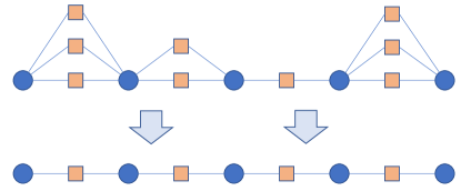
Figure 4: Factor graph for 1D surface reconstruction. Blue variable nodes are evenly spaced along the surface. Every consecutive pair is linked by a smoothness factor (orange, in line with the variable nodes); and where available, also by one or more measurement factors. Since all factors are linear, we combine all factors between a pair of variables into a single compound factor, to give the purely linear factor graph shown at the bottom.

 

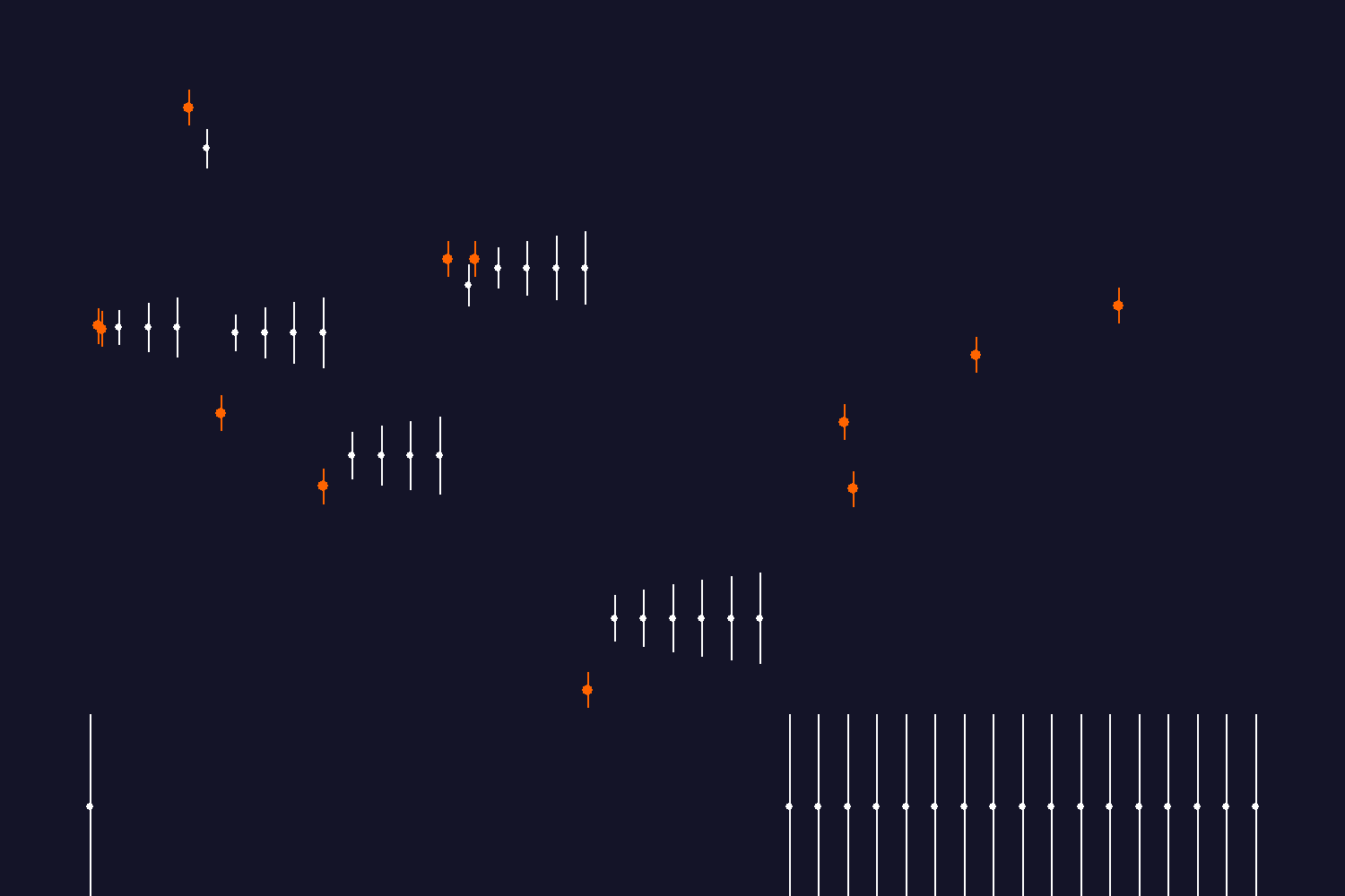
Floodfill 48 Floodfill 80 Floodfill 130 Floodfill 160

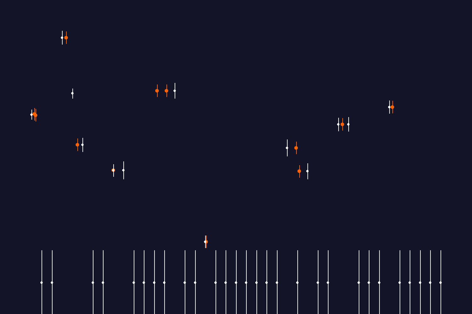
Random 243 Random 670 Random 2039 Random 5919

Figure 5: 1D surface fitting. Measurements are shown with their uncertainty as $\pm 1\sigma$ error bars in red, and 41 evenly spaced variable state estimates also with $\pm 1\sigma$ error bars in white. Each measurement defines a factor involving the two horizontally closest variables, and a smoothness factor also joins every pair of adjacent variables. Variables which have not yet received an informative message are initialised to a default zero value with large variance. The top row shows a serial floodfill message passing schedule, where variables and factors pass messages one by one, first from left to right and then back from right to left. The numbers mean the number of messages that have been passed. After 80, information has propagated all the way from left to right and we see the expected ‘open ended’ variable estimates which are only informed from the left. Messages return back from right to left and by 160 we have reached a full (equivalent to batch) solution, where we see each variable correctly influenced by both measurement and smoothness terms (with larger variances far from measurements). For comparison, the bottom row shows the worst case for message passing of a purely random schedule. At each step we randomly choose one of the 80 edges which connects a variable to a factor, and also randomly choose to pass a message either from factor to variable or from variable to factor. Clearly this is a very inefficient strategy, especially for a serial processor, and many messages must be passed; but eventually after several thousand random messages we reach the same globally correct solution.

 

In our first example, the goal is to reconstruct a height map surface from a set of point measurements. Each measurement has a perfectly known horizontal position, and Gaussian uncertainty in the vertical direction. We also have a Gaussian smoothness assumption over the surface.

We consider a one-dimensional height map here. We wish to estimate the surface heights at a quantised set of horizontal positions, and define a variable node for each of these. There are an abitrary number of measurements, each of which is associated with a factor node. The smoothness model is a Gaussian constraint on the relative height of every pair of consecutive variables, so there is another set of factor nodes joining these neighbours. The factor graph of this problem is visualised in Figure 4.

Each variable node $m_{i}$ has a fixed $x$ coordinate $x_{m_{i}}$, and a height $y_{m_{i}}$ to be estimated, and therefore a one-dimensional state variable space:

$${{\mathbf{x}}}_{m_{i}}=\left(\begin{array}[]{c}y_{m_{i}}\end{array}\right)~{}.$$ (74)

Each measurement has a fixed and perfectly known $x$ location $x_{s}$, and a scalar height measurement ${{\mathbf{z}}}_{s}=\left(\begin{array}[]{c}y_{s}\end{array}\right)$. All height measurements have a fixed measurement precision:

$${{\mathtt{\Lambda}}}_{s}=\left[\begin{array}[]{c}\frac{1}{\sigma_{m}^{2}}\end{array}\right]~{}.$$ (75)

A measurement at horizontal location $x_{s}$ is assumed to have a linearly interpolated dependence on the state variables having $x$ coordinates $x_{m_{1}}$ and $x_{m_{2}}$ which lie either side of it. We define:

$$\lambda_{s}=\frac{x_{s}-x_{m_{1}}}{x_{m_{2}}-x_{m_{1}}}$$ (76)

to be the fraction of the horizontal displacement between the two variable nodes at which the measurement applies, and therefore deduce the measurement function:

$${{\mathbf{h}}}_{s}({{\mathbf{x}}}_{m_{1}},{{\mathbf{x}}}_{m_{2}})=\left(\begin{array}[]{c}(1-\lambda_{s})y_{m_{1}}+\lambda_{s}y_{m_{2}}\end{array}\right)~{},$$ (77)

with Jacobian:

$${{\mathtt{J}}}_{s}=\left(\begin{array}[]{cc}1-\lambda_{s}&\lambda_{s}\end{array}\right)~{}.$$ (78)

Additionally, a simple smoothness factor is defined between every pair of consecutive variable nodes. We have:

$${{\mathbf{h}}}_{p}({{\mathbf{x}}}_{m_{1}},{{\mathbf{x}}}_{m_{2}})=\left(\begin{array}[]{c}y_{m_{2}}-y_{m_{1}}\end{array}\right)~{},$$ (79)

with scalar ‘measurement’ ${{\mathbf{z}}}_{p}=\left(\begin{array}[]{c}0\end{array}\right)$, Jacobian:

$${{\mathtt{J}}}_{p}=\left(\begin{array}[]{cc}0&-1\end{array}\right)~{},$$ (80)

and fixed precision:

$${{\mathtt{\Lambda}}}_{p}=\left[\begin{array}[]{c}\frac{1}{\sigma_{p}^{2}}\end{array}\right]~{}.$$ (81)

We linearise the factors, and for each pair of variables we can add any measurement factors containing them onto the smoothness factor which already connects them. This leads to a purely linear graph (variable to factor to variable to factor…) with no loops, and therefore GBP is known to converge perfectly with one pass in each direction.

We have implemented this example in a simple CPU Python simulator, with a measurement dataset read in from a text file and interactive graphics, available at http://www.doc.ic.ac.uk/ãjd/bp1d.py. The code requires a straightforward Python3 installation with NumPy for numerics and PyGame for interactive visualisation.

Figure 5 shows screenshots from the simulator, and the caption explains the progress of GBP estimation for two types of message passing schedule which represent the two extremes of efficiency for serial processing. In the top row of figures, we see a ‘floodfill’ scenario, where messages start from the leftmost variable and are passed one by one all the way along the chain of variables and factors to the far right, then all the way back. With one full traversal in both directions, all variables and factors are fully ‘informed’ from all parts of the graph, and we achieve the globally optimal solution. In the bottom row, we see the progress instead of a fully random message passing schedule, where many steps will incur wasted work if the variable or factor sending the message has not itself updated since its last message. However, the most interesting thing to observe here is that full convergence to the global optimum is still reliably reached after some thousand iterations, with purely random and distributable processing.

4.2 2D Pose Graph

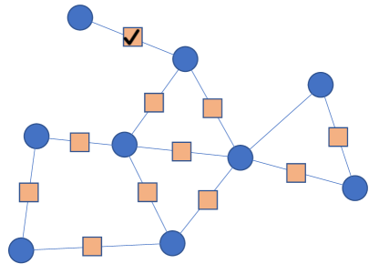
Figure 6: Factor graph for a 2D pose graph problem. Variable nodes (blue) scattered around the 2D plane are linked by randomly generated measurement factors (orange) between nearby nodes. Note that in our implementation we also use some absolute pose unary factors on the variables (one strong, to anchor one variable, the others very weak), which are not visualised here.

 

Our second example is a linear 2D pose graph, a simple version of the pose graph optimisation problem in mobile robotics where many robots or a single exploring robot must estimate their global locations from a network of purely relative measurements. This application of GBP is still linear, but now loopy, and therefore iterative message passing will certainly be needed to approach a global solution.

The factor graph under consideration is shown in Figure 6. In detail, each variable node has two degrees of freedom for its position on the 2D plane:

$${{\mathbf{x}}}_{m_{i}}=\left(\begin{array}[]{c}x_{m_{i}}\\ y_{m_{i}}\end{array}\right)~{}.$$ (82)

Each factor is a 2D Euclidean relative pose measurement ${{\mathbf{z}}}_{s}$ between two nodes, with measurement function:

$${{\mathbf{h}}}_{s}({{\mathbf{x}}}_{m_{i}},{{\mathbf{x}}}_{m_{j}})={{\mathbf{x}}}_{m_{j}}-{{\mathbf{x}}}_{m_{i}}~{},$$ (83)

and fixed measurement precision:

$${{\mathtt{\Lambda}}}_{s}=\left[\begin{array}[]{cc}\frac{1}{\sigma_{m}^{2}}&0\\ 0&\frac{1}{\sigma_{m}^{2}}\end{array}\right]~{}.$$ (84)

Measurement function ${{\mathbf{h}}}_{s}$ is linear so we only need to construct the linear constraint once. Given the Jacobian:

$${{\mathtt{J}}}_{s}=\left[\begin{array}[]{cccc}-1&0&1&0\\ 0&-1&0&1\end{array}\right]~{},$$ (85)

we construct information vector ${{\boldsymbol{\eta}}}_{s}$ and precision matrix ${{\mathtt{\Lambda}}}_{s}^{\prime}$ using Equation 36. Note that when the measurement function is linear as it is here, ${{\mathtt{J}}}_{s}{{\mathbf{x}}}_{0}={{\mathbf{h}}}_{s}({{\mathbf{x}}}_{0})$ and those two terms cancel out, so simply ${{\boldsymbol{\eta}}}_{s}={{\mathtt{J}}}_{s}^{\top}{{\mathtt{\Lambda}}}_{s}{{\mathbf{z}}}_{s}$.

We set up a simulation (code for our Python simulator is available from http://www.doc.ic.ac.uk/ãjd/bpmap.py). We define 20 variable nodes, which have randomly generated ground truth locations on the 2D plane. 50 measurements are also generated, each of which randomly connects two variable nodes, and which has a randomly generated measurement value sampled from a Gaussian distribution around the ground-truth value with precision ${{\mathtt{\Lambda}}}_{s}$. We also add a weak unary pose factor to each variable node. These factors have identity measurement functions and Jacobians. One chosen variable has a much stronger unary pose factor. This means that the whole network will be anchored.

So each variable node has zero or more randomly connected measurement factors. We visualise the progress of a simulated parallel message passing schedule in Figure 7, and discuss its progress in the caption, including a comparison with a full batch solution. This batch solution is formed by adding all linearised factors into a single large information matrix, and inverting this matrix to find the mean and covariance of all variables.

0 steps 1 step 2 steps

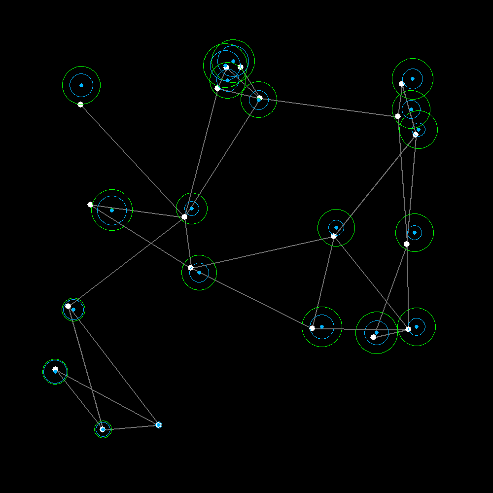
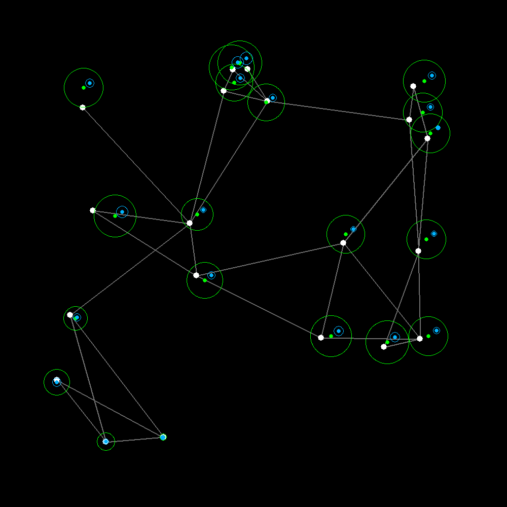
6 steps 171 steps Measurement Precision Increased

Figure 7: 2D linear pose graph, showing iterations of a random message passing scheme. The ground truth locations of variable nodes are shown in white, with estimates in blue (mean point locations and one sigma covariance as a circle). Each grey line is a measurement factor connecting two variables. There are 20 variable nodes and 50 measurements. Each variable also has a weak absolute pose factor, except for the anchored variable at the bottom centre of the scene which has a strong absolute pose factor, and these pose factors pass messages once to their variables at initialisation. Message passing then proceeds in the steps shown, simulating a parallel message schedule where at each step first every variable passes a message to all of the measurement factors it connects to, and then every measurement factor sends a message to every variable it connects to. In each sub-figure, on top of the incremental estimation we also show in green the batch solution to the full pose graph problem (mean point and one single covariance as a circle). We see that only a few steps are needed for the graph to reach good relative estimates (e.g. after 6 steps, where we see an almost constant shift between the GBP and batch solutions for nearby nodes). After 171 steps, information has fully propagated from the anchored node and the mean estimates from GBP are indistinguishable from the batch solution, though the covariances are in many cases overconfident. In the final panel we show that after convergence (or at any other time) we can make dynamic and local changes to the factors, the effects of which are transmitted to the whole graph with no changes to the GBP algorithm. Here we increase the precision of all measurement factors which changes the mean estimates because the weak pose factors are trusted less. (Note that we did not account for this in the green batch solution shown, which does not change.)

 

We observe that in this small graph, it takes a rather large number of iterations for the means to converge to estimates which are indistinguishable from the batch solution, but we should note that relative estimates in the graph are obtained after fairly few steps. For instance, if we look at the result after 6 steps in Figure 7, nodes nearby in the graph have mean estimates which differ from the batch solution by very similar offsets. At the stage the estimates in the graph are most likely highly useful for any application where relative information is important, such as robot navigation. The difference between 6 steps and 171 steps is that the rooted node with a strong pose factor is finally able to propagate absolute information around the whole graph. The covariances of the estimates are overconfident, which is a well known property of GBP, with generally greater overconfidence for nodes which are highly inter-connected graph regions.

In the final panel of the figure, we give an example of the extreme flexibility of GBP estimation, and the ability of decentralised estimation methods to work in an editable, reversible way. After convergence, we change the precision of all of the factor nodes to a stronger value, and the result of this quickly propagates through the graph, with no global coordination needed. Any number of dynamic changes like this can easily be dealt with, which we think will be important in the future of Spatial AI, where for instance some human input or machine learning process produces an updated value of a prior assumption (e.g. surface smoothness) which with most estimation methods would have become ‘baked into’ the representation.

4.3 Related Work

Pose graph optimisation is a heavily studied problem in robotics and computer vision, and the state of the art in academia is represented by excellent open source libraries such as g2o [20], GTSAM [13] and Ceres [3]. These libraries run on the CPU, and use methods such as sparse Cholesky decomposition to efficiently factorise the invert the information matrix of large problems. We make no claims that GBP is competitive with such methods on a CPU, because it requires many iterations. As noted before, the structure of doing processing with a CPU and unified memory storage allows ‘god view’ analysis of an optimisation problem and the determination of very efficient solvers. Presumably industry has in-house versions of these which are even more efficient.

Our argument in favour of GBP is about its suitability for different computing architectures such as graph processors with fully distributed processing and storage; and also its high flexibility and usefulness in handling the heterogeneous, always-changing graphs in Spatial AI. On hardware like a graph processor, our measure of what is an efficient algorithm needs to change from the CPU standard of total computation time. The performance of an algorithm on a graph processor depends on its need for distributed computation, storage and data tranmission, and probably a suitable measure should be multi-dimensional.

Within well known methods for CPU pose graph optimisation, the ones that are closest to GBP with a random message schedule are those based on Stochastic Gradient Descent, such as by Olson et al. [30] or Grisetti et al. [17]. We have not had the chance to make a head to head performance comparison with these first order methods, though GBP certainly has some appealing positive points even on the CPU, such as no need for the tuning of gain constants.

5 Robust Factors using M-Estimators

Most practical estimation methods in computer vision and robotics take account of the fact that sensors, especially outward-facing ones like cameras, have a measurement probability distribution which is not truly Gaussian. The classic behaviour is that the distribution is closely Gaussian when the sensor is essentially ‘working’, and reporting measurements that are close to ground truth apart from small variations due to quantisation and similar, but then some percentage of the time the sensor will report wildly incorrect ‘garbage’ measurements. For instance, if a camera is reporting the image location of matched image features, false correspondences happen sometimes and give measurements arbitrarily far away from ground truth. If we plot the measurement distribution of such a sensor we see a distribution which looks like a Gaussian centrally but is more ‘heavy-tailed’.

In optimisation and estimation, such behaviour is modelled using a family of ‘robust’ functions called M-Estimators. Here we will show that these robust functions can be easily incorporated into GBP with completely local processing.

Consider a standard measurement factor defined as in Equation 20 and linearised as in Equation 36. The form is:

$$f_{s}({{\mathbf{x}}}_{s})=Ke^{-\frac{1}{2}E_{s}}~{},$$ (86)

where $E_{s}$, the least squares ‘energy’ of the constraint, is:

$$E_{s}=({{\mathbf{z}}}_{s}-{{\mathbf{h}}}_{s}({{\mathbf{x}}}_{s}))^{\top}{{\mathtt{\Lambda}}}_{s}({{\mathbf{z}}}_{s}-{{\mathbf{h}}}_{s}({{\mathbf{x}}}_{s}))~{}.$$ (87)

The term:

$$M_{s}=\sqrt{({{\mathbf{z}}}_{s}-{{\mathbf{h}}}_{s}({{\mathbf{x}}}_{s}))^{\top}{{\mathtt{\Lambda}}}_{s}({{\mathbf{z}}}_{s}-{{\mathbf{h}}}_{s}({{\mathbf{x}}}_{s}))}$$ (88)

is the Mahalonobis distance, representing the number of standard deviations that the measurement is away from the mean of the distribution, and so for a standard Gaussian constraint we use a simple square $E_{s}=M_{s}^{2}$. In robust estimation, we vary this by setting a threshold level on $M_{s}$ beyond which we change the energy to a function which rises less steeply.

Let us first consider the commonly used Huber function which transitions from quadratic to a straight line beyond a threshold $M_{s}\geq N_{\sigma}$. A factor with Huber loss has the following form:

$$f_{s}({{\mathbf{x}}}_{s})=\begin{cases}Ke^{-\frac{1}{2}M_{s}^{2}}&\ M_{s}\leq N_{\sigma}\\ Ke^{-(N_{\sigma}M_{s}-\frac{1}{2}N_{\sigma}^{s})}&\ M_{s}\geq N_{\sigma}\end{cases}~{},$$ (89)

such that the two parts of the function match up in terms of both value and gradient at the discontinuity $M_{s}=N_{\sigma}$.

Now, in GBP, every message takes the form of an information vector and precision matrix representing a Gaussian distribution. So what we do to represent the effect of the non-Gaussian part of a robust factor is to find the Gaussian distribution which has the same value energy, and pass a message with that precision instead. This is similar to the Dynamic Covariance Scaling method in [2]. We ask what Mahalonobis distance we must be from the mean in a standard quadratic energy to be equivalent to the Huber energy in the linear region. Specifically, we need to find $M_{sR}$ such that:

$$\frac{1}{2}M_{sR}^{2}=N_{\sigma}M_{s}-\frac{1}{2}N_{\sigma}^{s}~{}.$$ (90)

Rearranging we find:

$$M_{sR}=\sqrt{2N_{\sigma}M_{s}-N_{\sigma}^{2}}~{}.$$ (91)

And therefore:

$$k_{R}=\frac{M_{sR}^{2}}{M_{s}^{2}}=\frac{2N_{\sigma}}{M_{s}}-\frac{N_{\sigma}^{2}}{M_{s}^{2}}$$ (92)

is the factor by which the energy of the constraint should be reduced. Remembering the information form of Equation 25, we see that this is achieved by multiplying both the precision matrix ${{\mathtt{\Lambda}}}_{s}^{\prime}$ and information vector ${{\boldsymbol{\eta}}}_{s}$ by this factor.

So, to summarise, to use a Huber norm on a factor, every time that factor is to pass a message we first use all the latest incoming messages from variables in order to form its state vector ${{\mathbf{x}}}_{s}$, and then evaluate the current Mahalonobis distance $M_{s}$ using Equation 88. We test this against the $N_{\sigma}$ cutoff we have set for this factor (which might be 4.0 or something similar), representing the number of standard deviations from the mean for which we expect Gaussian behaviour. If $M_{s}\leq N_{\sigma}$ we are in the Gaussian zone and use the standard linearised precision matrix and information vector for the message calculate. If $M_{s}\geq N_{\sigma}$, we temporarily scale ${{\mathtt{\Lambda}}}_{s}^{\prime}$ and ${{\boldsymbol{\eta}}}_{s}$ by factor $k_{R}$ as calculated in Equation 92 for the purposes of this message pass only.

We can use the same method to handle other robust norms. For instance, a function which is Gaussian up to $M_{s}\leq N_{\sigma}$ and then constant beyond is implemented with a factor $k_{R}=\frac{N_{\sigma}^{2}}{M_{s}^{2}}$.

We will see that these robust factors allow lazy data association during GBP (reminiscent of [29]), where the robust status of factors can change dynamically during ongoing graph optimisation, giving the ability to reject poor measurements immediately or after enough contradictory alternative data has been received.

An interesting future area for research is a multi-modal approach where we might initialise multiple robust factors with different precision values to represent a single measurement, and allow them to ‘fight it out’ over iterations of BP to find the best supported hypothesis, and achieving a discrete model-selection capability.

6 Incremental SLAM

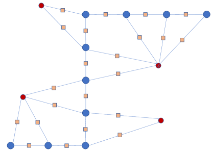
Figure 8: Factor graph for a 2D SLAM problem. Blue nodes are variable nodes describing the robot position while red nodes are landmark variable nodes. The orange squares are factors representing 2D constraints.

 

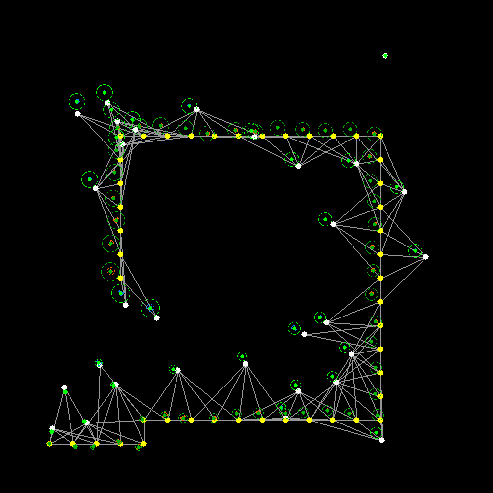
Early exploration Just before loop closure

Just after loop closure Steady state convergence

Figure 9: 2D SLAM simulation. A moving ‘robot’, with history of ground truth poses shown as yellow dots, explores a scene with containing landmarks (ground truth positions are white dots), and from each pose makes observations of nearby landmarks to incrementally build the factor graph shown in grey. Red and blue dots and ellipses show the robot and landmark estimates obtained from GBP, which runs continually on the growing factor graph. We also superimpose the optimal batch solution to the graph in green for comparison. We see close agreement between the GBP and batch estimates until loop closure occurs, where the large correction needed takes a large number of GBP iterations to propagate fully around the graph. However, even very soon after loop closure we see that the relative information in the GBP estimate is good, with nearby nodes having estimates differing from the batch solution by similar amounts.

 

We will now show how GBP can be straightforwardly applied to an ever-changing SLAM graph, including the optional use of robust factors to account for poor data association.

6.1 Incremental SLAM with Standard Gaussian Factors

First we will tackle incremental SLAM but using standard Gaussian factors. We simulated a 2D cartesian SLAM problem, where as a ‘robot’ translates it leaves a history of pose variable nodes, with each consecutive pair joined by a factor on their relative locations representing a measurement from odometry (see Figure 8). Scattered throughout the simulated 2D environment are landmarks the robot can observe. From each new robot pose, factors are added to the graph to represent measurements of the landmarks withing a bounded distance. All measurements in the simulation have randomly sampled Gaussian noise, using different but constant covariances for the odometry factors and measurement factors respectively; the factors in the graph are initialised with the corresponding precision matrices. There is no rotation in the simulation, and all measurements are in cartesian space, so this is again a formulation where the dependence of measurements on variables is purely linear, and the mathematical details of variable and factor message passing are the same as in the 2D constraint graphs of Section 4.2. We have a strong pose factor attached to the first robot variable node, anchoring this node and effectively defining the coordinate frame for SLAM.

We visualise the progress of SLAM estimation in Figure 9. In our simulation, which is available from http://www.doc.ic.ac.uk/ãjd/bpslam.py, keyboard controls w,a,s,d can be used to move the robot, and the factor graph is generated automatically and incrementally. In the background, we run a continuous schedule of simulated parallel message passing. At each step, all variables use their waiting incoming messages to calculate outgoing messages to all connected factors. Then, in alternation, all factors do the same thing. The variables and factors in the dynamically changing graph are stored in dynamic vector data structures and we can easily iterate through all of them as the vectors grow. The figure shows that we make SLAM estimates which are consistent with a batch solution, and that GBP can comfortably cope with the dynamically changing graph, including major events such as loop closure.

6.2 Incremental SLAM with Robust Factors

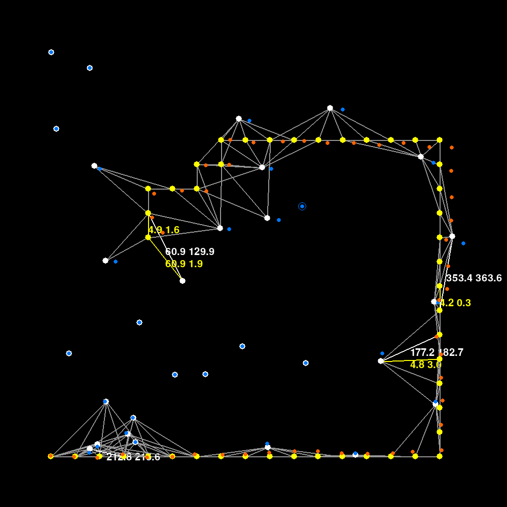
New erroneous measurement (red) Second measurement of landmark Further good measurements; error rejected

White and yellow factors balance error Erroneous factor is white; others grey

Loop closure Comparison with non-robust After more measurements,

batch solution (green) 4 outliers confidently identified

Figure 10: 2D SLAM simulation with random erroneous measurements and robust factors. Every time a factor passes a message, it reevaluates its Mahalonobis distance. In this simulation, we use a Huber loss with Mahalonobis distance threshold of 4.0 to transition from quadratic to linear cost. One in 50 ground truth measurements in the simulation has a large error added. In the visualisation, factors are colour-coded: grey if the Mahalonobis distances of both the ground truth measurement and the current factor estimate are both below 4.0 (normal case); white if both distances are above 4.0 (an erroneous measurement that BP has recognised as such and is treating with the linear part of the Huber function; red for a factor with high ground truth distance but low in the factor: this is an erroneous measure not yet recognised; and yellow for a factor with high factor distance but low ground truth distance; this is a good measurement being ‘unfairly’ treated as an outlier. All non-grey factors display their estimated and true Mahalonobis distances numerically. When a first erroneous measurement is made to initialise a new landmark, there are no contradictory good measurements to oppose it. In the second and third panels, additional measurements of the landmark support each other and push the erroneous measurement far into the linear Huber region. Good estimates are seen throughout the graph after loop closure, and a much better result than the green batch solution which does not take account of outliers (of course, we could have used robust methods there as well). More exploration and further loop closure happens by the last panel, and four erroneous measurements are now very confidently identified.

 

In Figure 10 we now see the performance of GBP for incremental SLAM when a random $\frac{1}{50}$ of all measurements have a large error added, and all factors now use a robust Huber kernel. This can be tried out as part of the same simulation http://www.doc.ic.ac.uk/ãjd/bpslam.py, pressing ‘r’ to enter robust mode. GBP with robust factors has the impressive capability to detect outlier measurements in a local and lazy manner, with erroneous measurements which were not immediately apparent often determined much later when enough support builds up for a better hypothesis. Playing with the simulator is the best way to get a good feel for this.

6.3 Towards Front-End Use

Our example here of SLAM with robust factors shows how errors that slip through the front-end measurement part of a SLAM system (such as visual feature matching) could be cleaned up by back-end estimation. In the longer term, we are interested in how GBP and graph-based estimation could be used for the whole of a Spatial AI system, including front-end data association like the matching in a sparse or dense SLAM system, avoiding the need for ad-hoc algorithms such as RANSAC. We believe that this will be possible, and plan to experiment further soon. For instance, in dense SLAM data associate (such as the ICP tracking in KinectFusion [28]), each pixel measurement from a depth camera is associated with several possible locations in a dense model, and this association is refined iteratively through ICP. We could replace this process with GBP, where the measurement might be connected by several factors to different scene points, with mutually exclusive robust factors whose different means would fight it out via GBP, in collaboration with other inter-measurement factors representing smoothness, etc., until the most probably associations are reached. This could be something which could be efficiently implemented on a distributed close-to-the-sensor processor.

7 GBP Convergence Properties and Message Schedules

In this paper, we have focused on the local details of GBP, and shown various examples, and it is not within our current scope to examine the large scale properties of the algorithm. In fact, previously published implementations and some of our own as-yet unpublished experiments are very promising, though there are still many open questions.

The most common impression of GBP in extended, loopy linear problems is that it converges to correct means with overconfident covariances, and this is certainly what we have observed in our example implementations. The covariance overconfidence we observe can be most easily understood in Malioutov et al.’s Walk Sum Framework [22] in which the loopy graph is unrolled into a computation graph that is a tree. It is remarkable that the means in loopy GBP converge to correct values even when the covariances are overconfident [44]. This means that the precisions on the incoming messages that each variable receives must be in the correct proportions. Per variable node, there must be constant factor by which the incoming messages at convergence are stronger than they should be. Can we back this observation out to the factors and the whole graph, and then understand how to correct for overconfidence? A clear empirical pattern is that overconfidence is greater for nodes in densely connected parts of a graph, where messages will travel over very loopy, self-reinforcing paths. Perhaps some simple heuristics would be able to describe the behaviour well even without a full theory. We recall iSAM2 [19], where message passing is restricted to the spanning of a graph tree so that marginal covariance estimates are conservative. Maintaining the spanning tree is however not a local operation.

Importantly, it is known that loopy linear GBP does not always converge. More specifically, previous authors have found that while the marginal covariances will always converge to the same values given a positive semi-definite message information matrix initialisation [14], whether or not the means will converge depends on the spectral radius of the linear system for the means that is formed after convergence of the covariances. It has been shown that message damping can improve convergence in these situations [22]. In message damping, at each message passing step the calculated message is combined in a fixed weighted ratio with the previous message sent along that particular edge.

Different issues arise in non-linear problems, where factors must be repeatedly relinearlised. Clearly, one strategy is to delay relinearisation, such that with a chosen linearisation for each factor we iterate message passing until convergence, with the same properties as any linear problem, and then relinearise everything and repeat. More aggressive local relinearisation is attractive, because each factor is always using its current estimates to linearise, but we are not yet sure of the effect of this on global convergence. Dynamically changing the factors as we do in our technique for using robust kernels does not seem to cause any unstability in optimisation.

When it comes to message schedules for GBP, beyond the first 1D example in Section 4.1 where we showed a sequential floodfill schedule, we have focused on schedules which can be implemented in purely parallel architectures, in the simplest way such that every variable sends messages, then every factor sends messages.

Such a schedule is sometimes obviously inefficient, for instance in transmitting absolute pose information which is available only at one node throughout the whole graph, which happens in very slow steps, and most of the graph is churning away in parallel for many iterations without much changing. A good question is to what extent this could be improved on without needing global knowledge of the structure of the graph. Certainly, at a local level, individual nodes could decide only to come alive and pass messages when their incoming messages have changed by a significant enough amount, perhaps judged using information theoretic measures [11]. This is reminiscent of the ‘Wildfire’ algorithm in Loopy SAM [33]. Information theoretic measures will also be crucial in the longer term in deciding on the number of bits needs to specify the quantities used in message passing.

However, thoughts about message schedules should take into account our interest in GBP as part of Spatial AI, where the graphs of interest are always dynamically changing; and where factors and variables may have many heterogeneous forms and connection patterns. We foresee systems where messages passing takes place continuously as the graph grows, changes, and sometimes simplifies, and perhaps never or rarely reaches global convergence. Factors may exist which have very long-reaching effects, due to recognition of large structures for instance, and these may have very good properties for global estimation even with few iterations. Most fundamentally, we believe that the ‘master representation’ of our approach should be the factor graph itself, and that all marginal estimates due to message passing are ultimately ephemeral, reversible and that most estimates of interest are recomputable locally if needed. Therefore a standard analysis of convergence may not be the most important property.

8 Towards Fully Graph-Based Spatial AI

Let us get back to the vision we suggested in the introduction of this paper, where all or most of the storage and processing for real-time Spatial AI is carried out in a purely distributed way, suitable for novel architectures such as graph processors, or even loose constellations of independent communicating devices. Probabilistic, geometric estimation as enabled by GBP must be combined with learned recognition capabilities to produce semantically meaningful representations. There is certainly great potential for full integration with the increasingly important and developed area of Geometric Deep Learning [7], which operates on graph data by design, and the promise of fully graph-based semantic SLAM systems. Clusters of related, linked nodes can be recognised as objects or other high level entities by a graph neural network. New factors which impose the regularity (e.g. smoothness) of these entities can be added and incorporated into GBP.

If confidence is high enough, recognised node clusters can be simplified into more efficient parametrised representations, by combining many nodes into object supernodes, or even hierarchies of these. We believe that the destiny of a Spatial AI graph representation is to become a sparse object graph as in SLAM++ [36]. In fact, this simplification is essential, for if we are to retain a factor graph as our master representation of a scene, and store and update it in real-time on a practical embedded processor, the size of a graph must remain bounded. As new measurements from live sensors in a dynamic scene flow in, the graph must be repeatedly abstracted and simplified to remain finite. Recognition of higher level entities could come from outside the graph (such as from a CNN running on input images). Or, for processing to remain truly distributed, it would occur locally, within the graph, from learned and geometric graph-based measures.

Meanwhile, can local changes and abstraction lead towards a graph with the right global properties to stay useful? Ideally, we believe that a Spatial AI graph should have ‘small world’ properties, such that a path exists between any two nodes which has a bounded number of edge hops, and therefore that information flow and optimisation can always happen efficiently. To what extent are we able to build such a structure into a graph, and for that structure not to be purely a representation of the simplest compilation of measurement data?

We will consider these issues in a little more detail in the following sections.

8.1 Recognition, Semantics and Objects

In GBP, it is trivial to take a set of variable nodes and merge them into a single supernode. The supernode has a state vector which is the concatenation of the individual variable states. All factors which were connected to the individual variables now connect to the supernode, with appropriate sparse measurement functions and Jacobians to reference the right variables. Any factors between variables which have all been joined into the supernode become new unary factors.

However, we do not gain much advantage by just joining nodes like this; message passing through the supernode becomes expensive because large matrices must now be manipulated due to its large state and large number of connections to factors. The benefits occur if we can simplify the state representation of the supernode to something much smaller. For example, imagine a set of variables representing points on a surface which are joined together because a recognition module has identitied the surface as a plane. If we are confident enough about this, we can replace the many point coordinates by the parametric equation of an infinite plane, which can be represented with only three parameters (this is reminiscent of [35]). All factors connected to the supernode could then be transformed to relate to these parameters. As it stands, the supernode would still have a very large number of factors connecting it to all the other parts of the graph which connected to the original variables. However, if these other graph parts are gradually simplified too, factors can be combined together and the number of connections will also reduce greatly. For instance, if the planar surface region has been observed by a moving camera over a long period of time, and each historic camera position is represented by an individual variable node, in our factor graph each of these camera variables will be connected to the plane supernode. However, it may be that the relative locations of the camera variable nodes at some point become so well known and this section of the graph so locally ‘rigid’ that we can also replace all of those nodes with a simpler entity such as a ‘trajectory segment’ supernode, the many factors linking to it to the plane could be summarised and combined into efficient ‘superfactors’.

The precise implementation details of such operations are still to be worked out, but we find this direction very convincing. Some interesting recent papers on non-linear factor recovery [24, 42] may provide useful tools for summarising parts of a graph with new superfactors which retain a non-linear form, and this is consistent with our picture of keeping the factor graph as the master representation.

We should be clear that combining nodes into simpler entities is difficult or impossible to reverse, unlike most of the processing we do in GBP. However, making greedy assumptions and simplifying representations must ultimately be an essential part of efficient intelligence, and something that biological brains do as proven by optical illusions.

8.2 Overall Structure

A related area for research, as graphs grow larger with more measurements and variables, but also incrementally become abstracted and simplified, is how the whole graph should be laid out with respect to computing hardware, and whether the whole graph structure enables efficient global or just-in-time inference of properties of interest.

On a graph processor such as Graphcore’s IPU, which has distributed graph computation but is still at heart a synchronous processor with global clocking and coordination, a significant issue is that the structure of the computation graph must normally be decided and fixed at compile time. With dynamic Spatial AI graphs, the most obvious option is to precompile a graph structure which we estimate is ‘big enough’ for the problem of interest, and then to fill that structure up dynamically at run-time. We believe that this is both feasible and practical. We could perform analysis of the typical graphs we would ideally build in an off-line experiment, and measure the typical number of nodes and amount of interconnectivity and use these to choose parameters of the pre-defined graph. Of course this need for graph compilation may go away with alternative future hardware.

Another interesting issue relates to our observation (e.g. in Figure 7) that in SLAM-like problems with mainly relative measurements, GBP will often produce good relative estimates rather quickly while it can take many iterations are needed to get good absolute estimates. In many applications, it is only the relative information which is important (for a robot which needs to plan its next actions to avoid obstacles for instance), and this raises the question of whether a different parametrisation which is relative by definition would be more suitable. This question has been considered before, such as in Sibley et al.’s Relative Bundle Adjustment [37], where all scene points were represented relative to a camera pose, and loop closure could happen as a simple connection operation with the option for global adjustment only if needed. These methods deserve being looked at again, though we wonder still how well they generalise to general graphs and motion rather than the ‘corridor-like’ trajectories of cameras they were originally devised for.

8.3 Active Processing and Attention

If a whole graph is stored within a graph processor, it can be operated on via GBP ‘in place’, and potentially all parts of the graph could circulate messages at the same rate (as in our SLAM examples). However, it is unlikely that this would make sense in terms of power efficiency, and that there are likely to be parts of the graph which are currently of much more interest which will be a priority for processing — most obviously, at the current location of a moving device or robot which is making current sensor measurements and must decide on action. Processing ‘attention’ could actively be focused on this area with a high rate of message passing, while other parts of the graph are partially or completely neglected, to be picked up and updated later on as needed ‘just in time’. We imagine an attention spotlight which moves around the graph, bringing it to life.

Depending on memory constraints (and current graph processors do not have a huge amount of on chip memory, e.g. around 300MB for one Graphcore IPU), graph regions out of the current attention spotlight might even be much abstracted and simplified to low resolution, approximated forms maintaining only the main shape and connectivity, perhaps in an analogue of the way that a human brain remembers distant places. When a moving device with data-rich sensors such as cameras revisits these places, they can easily feed on this data to be brought back to the high resolution needed for local action.

There may need to be a particular region of a graph processor held aside as the current active workspace, where enough precompiled space is retained such that the live part of the graph can be copied, unpacked and subject to full rate processing (the Real-Time Loop part of the ‘Spatial AI Brain’ shown in Figure 4 of [12]). Major processing elements such as a semantic labelling deep network could be held to run permanently here, only to operate on live image data (if such a network has many weights then it would not be possible in any case to distribute many copies of those weights around the whole graph so that labelling could happen in any location).

Between the active workspace and the rest of the graph there will need to be some special graph infrastructure such as routing nodes to interface between live workspace and long-term graph memory.

8.4 Graphs of Multiple Communicating Devices

In the final part of this speculative section, we consider the strong prospects for GBP methods to be used outside of the confines of a single graph processor, to connect many independent but intercommunicating devices such that they can jointly estimate global quantities. Individual devices will have their own individual estimation algorithms, sensors and hardware, but could use GBP as the general ‘glue language’ to share probabilistic information and come to agreement over global estimation matters, such as if a swarm of robotic devices were to be organised into a regular grid via only local computation and communication.

What will be important to achieve such capabilities will be standards for interoperation and messages which can be deployed for communication. Inspired by the creation of the World Wide Web [4], we believe that a fairly limited set of open communication standards which are the equivalent of HTTP, HTML, URL, etc. could define how devices could send probabilistic messages to each other while each maintains and runs its own internal operation in whichever proprietory way is desired. Such a set of standards could be the most important way that GBP becomes influential, as a standard for distributed estimation, rather than it being instantiated in monolithic libraries like other estimation methods.

9 Conclusions

We have presented a detailed case for a serious reconsideration of Gaussian Belief Propagation in Spatial AI, inspired chiefly by the current rapid developments in processor hardware which open up the chance to close the large gap between the requirements for advanced perception on embodied intelligent products and what can be delivered with practical mass-market, low-power technology. The advantage will increasingly be with algorithms which can take advantage of purely distributed processing and storage but still deliver globally meaningful estimates of the properties of a device and its surroundings.

A non-linear factor graph is the purest representation of probabilistic knowledge from multiple heterogeneous information sources, and can be efficiently stored and dynamically edited as the master representation for Spatial AI. Gaussian Belief Propagation is the simple but highly flexible tool which can turn a factor graph into a set of marginal probabilistic estimates with flexible distributed processing and storage, suitable either for graph processor chips or networks of individual devices with pairwise communication. We imagine large real-time systems operating with continual or attention-focused processing on their dynamic factor graphs, perhaps never reaching full estimation convergence but with estimates always good enough to be useful, either locally or globally, or intensively calculated on demand in a just-in-time manner. More specifically designed algorithms and specialised computing hardware for these will always exist for focused uses, but GBP can serve as a general ‘glue’ which holds all of these together in a rigorous probabilistic framework. An important systems focus will be the definition of interfaces which allow multiple devices to pass messages between them.

The factor graph in such a system must be kept bounded, and we believe that the route towards this is continual graph-based introspection to discover regions and structures which can be simplified by deleting or merging nodes. These mechanisms should interface with learned graph-based recognition mechanisms which identify and segment objects or simple structures which can be efficiently parameterised.

There are clearly many open questions in this research area, especially related to the convergence of estimation in large graphs, where there is much research and new theories needed. We have enough confidence in the potential of GBP methods for Spatial AI to believe that it is worth spending the many years needed on the research to take them into practical systems. This is an algorithmic framework ready not just for processor types already in production, but even more exotic future possibilities such as neuromorphic devices which give up on global timing and synchronisation.

References

- [1] Graphcore. URL https://www.graphcore.ai/.
- [2] P. Agarwal, G. D. Tipaldi, L. Spinello, C. Stachniss, and W. Burgard. Robust map optimization using dynamic covariance scaling. In Proceedings of the IEEE International Conference on Robotics and Automation (ICRA), 2012.
- [3] S. Agarwal, M. K., and Others. Ceres solver. http://ceres-solver.org.
- [4] T. Berners-Lee. Weaving the Web: The Original Design and Ultimate Destiny of the World Wide Web. Harper, 1999.
- [5] C. M. Bishop. Pattern Recognition and Machine Learning. Springer-Verlag New York, Inc., 2006.
- [6] M. Bloesch, J. Czarnowski, R. Clark, S. Leutenegger, and A. J. Davison. CodeSLAM — learning a compact, optimisable representation for dense visual SLAM. In Proceedings of the IEEE Conference on Computer Vision and Pattern Recognition (CVPR), 2018.
- [7] M. M. Bronstein, J. Bruna, Y. LeCun, A. Szlam, and P. Vandergheynst. Geometric Deep Learning: Going beyond Euclidean data. IEEE Signal Processing Magazine, 34(4):18–42, 2017.
- [8] A. Chambolle and T. Pock. A First-Order Primal-Dual Algorithm for Convex Problems with Applications to Imaging. Journal of Mathematical Imaging and Vision, 40(1):120–145, 2011.
- [9] S. Choudhary, L. Carlone, C. Nieto, J. Rogers, H. Christensen, and F. Dellaert. Distributed mapping with privacy and communication constraints: Lightweight algorithms and object-based models. International Journal of Robotics Research (IJRR), 36(12):1286–1311, 2017.
- [10] D. Crandall, A. Owens, N. Snavely, and D. Huttenlocher. Discrete-continuous optimization for large-scale structure from motion. In Proceedings of the IEEE Conference on Computer Vision and Pattern Recognition (CVPR), 2011.
- [11] A. J. Davison. Active Search for Real-Time Vision. In Proceedings of the International Conference on Computer Vision (ICCV), 2005.
- [12] A. J. Davison. FutureMapping: The computational structure of Spatial AI systems. arXiv preprint arXiv:arXiv:1803.11288, 2018.
- [13] F. Dellaert and M. Kaess. Factor Graphs for Robot Perception. Foundations and Trends in Robotics, 6(1–2):1–139, 2017.
- [14] J. Du, S. Ma, Y.-C. Wu, S. Kar, and J. M. Moura. Convergence analysis of distributed inference with vector-valued gaussian belief propagation. Journal of Machine Learning Research, 18:172–1, 2017.
- [15] J.-J. Engel. Large-Scale Direct SLAM and 3D Reconstruction in Real-Time. PhD thesis, 2017.
- [16] R. M. Eustice, H. Singh, and J. J. Leonard. Exactly Sparse Delayed State Filters. In Proceedings of the IEEE International Conference on Robotics and Automation (ICRA), 2005.
- [17] G. Grisetti, C. Stachniss, and W. Burgard. Non-linear constraint network optimization for efficient map learning. IEEE Transactions on Intelligent Transportation Systems, 10(3):428–439, 2009.
- [18] E. T. Jaynes. Probability Theory: The Logic of Science. Cambridge University Press, 2003.
- [19] M. Kaess, H. Johannsson, R. Roberts, V. Ila, J. Leonard, and F. Dellaert. iSAM2: Incremental Smoothing and Mapping Using the Bayes Tree. International Journal of Robotics Research (IJRR), 2012. To appear.
- [20] R. Kümmerle, G. Grisetti, H. Strasdat, K. Konolige, and W. Burgard. : A General Framework for Graph Optimization. In Proceedings of the IEEE International Conference on Robotics and Automation (ICRA), 2011.
- [21] S. Leutenegger, S. Lynen, M. Bosse, R. Siegwart, and P. Furgale. Keyframe-based visual-inertial odometry using nonlinear optimization. The International Journal of Robotics Research, 34(3):314–334, 2014.
- [22] D. M. Malioutov, J. K. Johnson, and A. S. Willsky. Walk-sums and belief propagation in Gaussian graphical models. Journal of Machine Learning Research, 7(Oct):2031–2064, 2006.
- [23] J. Martel. Unconventional Processing with Unconventional Visual Sensing. PhD thesis, ETH Zurich, 2019.
- [24] M. Mazuran, W. Burgard, and G. D. Tipaldi. Nonlinear factor recovery for long-term SLAM. International Journal of Robotics Research (IJRR), 35(1):50–72, 2016.
- [25] J. McCormac, A. Handa, A. J. Davison, and S. Leutenegger. SemanticFusion: Dense 3D semantic mapping with convolutional neural networks. In Proceedings of the IEEE International Conference on Robotics and Automation (ICRA), 2017.
- [26] A. I. Mourikis and S. I. Roumeliotis. A multi-state constraint Kalman filter for vision-aided inertial navigation. In Robotics and Automation, 2007 IEEE International Conference on, pages 3565–3572. IEEE, 2007.
- [27] R. A. Newcombe. Dense Visual SLAM. PhD thesis, Imperial College London, 2012.
- [28] R. A. Newcombe, S. Izadi, O. Hilliges, D. Molyneaux, D. Kim, A. J. Davison, P. Kohli, J. Shotton, S. Hodges, and A. Fitzgibbon. KinectFusion: Real-Time Dense Surface Mapping and Tracking. In Proceedings of the International Symposium on Mixed and Augmented Reality (ISMAR), 2011.
- [29] E. Olson and P. Agarwal. Inference on networks of mixtures for robust robot mapping. International Journal of Robotics Research (IJRR), 32(7):826–840, 2013.
- [30] E. Olson, J. J. Leonard, and S. Teller. Fast iterative alignment of pose graphs with poor initial estimates. In Proceedings of the IEEE International Conference on Robotics and Automation (ICRA), 2006.
- [31] M. A. Paskin. Thin Junction Tree Filters for Simultaneous Localization and Mapping. In Proceedings of the International Joint Conference on Artificial Intelligence (IJCAI), 2003.
- [32] J. Pearl. Reverend Bayes on inference engines: A distributed hierarchical approach. In Proceedings of the National Conference on Artificial Intelligence (AAAI), 1982.
- [33] A. Ranganathan, M. Kaess, and F. Dellaert. Loopy SAM. In Proceedings of the International Joint Conference on Artificial Intelligence (IJCAI), 2007.
- [34] S. Saeedi, M. Trentini, M. Seto, and H. Li. Multiple-robot Simultaneous Localization and Mapping — A Review. Journal of Field Robotics (JFR), 33(1):3–46, 2016.
- [35] R. F. Salas-Moreno, B. Glocker, P. H. J. Kelly, and A. J. Davison. Dense planar SLAM. In Proceedings of the International Symposium on Mixed and Augmented Reality (ISMAR), 2014.
- [36] R. F. Salas-Moreno, R. A. Newcombe, H. Strasdat, P. H. J. Kelly, and A. J. Davison. SLAM++: Simultaneous Localisation and Mapping at the Level of Objects. In Proceedings of the IEEE Conference on Computer Vision and Pattern Recognition (CVPR), 2013.
- [37] G. Sibley, C. Mei, I. Reid, and P. Newman. Adaptive Relative Bundle Adjustment. In Proceedings of Robotics: Science and Systems (RSS), 2009.
- [38] H. Strasdat, J. M. M. Montiel, and A. J. Davison. Real-Time Monocular SLAM: Why Filter? In Proceedings of the IEEE International Conference on Robotics and Automation (ICRA), 2010.
- [39] E. B. Sudderth, M. J. Wainwright, and A. S. Willsky. Embedded trees: Estimation of Gaussian processes on graphs with cycles. IEEE Transactions on Signal Processing, 52(11):3136–3150, 2004.
- [40] H. Sutter. Welcome to the jungle. URL https://herbsutter.com/welcome-to-the-jungle, 2011.
- [41] B. Triggs, P. McLauchlan, R. Hartley, and A. Fitzgibbon. Bundle Adjustment — A Modern Synthesis. In Proceedings of the International Workshop on Vision Algorithms, in association with ICCV, 1999.
- [42] V. Usenko, N. Demmel, D. Schubert, J. Stückler, and D. Cremers. Visual-inertial mapping with non-linear factor recovery. arXiv preprint:1904:11781, 2019.
- [43] C. S. Weerasekera, T. Dharmasiri, R. Garg, T. Drummond, and I. D. Reid. Just-in-Time Reconstruction: inpainting sparse maps using single view depth predictors as priors. In Proceedings of the IEEE International Conference on Robotics and Automation (ICRA), 2018.
- [44] Y. Weiss and W. T. Freeman. Correctness of belief propagation in Gaussian graphical models of arbitrary topology. In Neural Information Processing Systems (NIPS), pages 673–679, 2000.
- [45] T. Whelan, S. Leutenegger, R. F. Salas-Moreno, B. Glocker, and A. J. Davison. ElasticFusion: Dense SLAM without a pose graph. In Proceedings of Robotics: Science and Systems (RSS), 2015.
- [46] C. Wu, S. Agarwal, B. Curless, and S. M. Seitz. Multicore Bundle Adjustment. In Proceedings of the IEEE Conference on Computer Vision and Pattern Recognition (CVPR), 2011.
- [47] S. Zhi, M. Bloesch, S. Leutenegger, and A. J. Davison. SceneCode: Monocular dense semantic reconstruction using learned encoded scene representations. In Proceedings of the IEEE Conference on Computer Vision and Pattern Recognition (CVPR), 2019.
- [48] J. Zienkiewicz. Dense Monocular Perception for Mobile Robotics. PhD thesis, Imperial College London, 2017.