Unsupervised inference approach to facial attractiveness

Abstract

The perception of facial beauty is a complex phenomenon depending on many, detailed and global facial features influencing each other. In the machine learning community this problem is typically tackled as a problem of supervised inference. However, it has been conjectured that this approach does not capture the complexity of the phenomenon. A recent original experiment (Ibáñez-Berganza et al., Scientific Reports 9, 8364, 2019) allowed different human subjects to navigate the face-space and “sculpt” their preferred modification of a reference facial portrait. Here we present an unsupervised inference study of the set of sculpted facial vectors in that experiment. We first infer minimal, interpretable, and faithful probabilistic models (through Maximum Entropy and artificial neural networks) of the preferred facial variations, that capture the origin of the observed inter-subject diversity in the sculpted faces. The application of such generative models to the supervised classification of the gender of the sculpting subjects, reveals an astonishingly high prediction accuracy. This result suggests that much relevant information regarding the subjects may influence (and be elicited from) her/his facial preference criteria, in agreement with the multiple motive theory of attractiveness proposed in previous works.

1 Introduction

Human facial perception (of identity, emotions, personality dimensions, attractiveness [1, 2, 3]) has been the subject of an intense and multidisciplinary research in the last decades. In particular, facial attractiveness is a research topic in many different disciplines, from evolutionary biology and psychology to neuroscience [4, 5, 6, 7, 8]. Furthermore, it is an interesting case of study in the machine learning research community, as a paradigm of a complex cognitive phenomenon, ruled by complex and difficult to infer criteria. Indeed, the rules according to which a facial image will probably result pleasant to an individual or in average, are poorly known [2, 6]. The most relevant face-space variables in terms of which such rules should be inferred remain elusive as well [6].

In the context of evolutionary biology, on the one hand, many works have discussed the validity of the so called natural selection hypothesis [2]. Despite the success of the natural selection hypothesis, it is believed that it does not take into account the phenomenon in its various complex facets. Indeed, important cultural and inter-person differences, beyond the species-typical criterion, are known to influence facial attractiveness [7]. On the other hand, the main goal of the machine learning approach is the automatic rating of facial images, as a supervised inference problem [6]. The facial image is parametrised in a face-space vector ${\bf f}$, the inference goal consists in inferring the model $R({\bf f})$ that reproduces at best the subject-averaged ratings $\langle R_{s}\rangle_{s}$ of a database $\{{\bf f}_{s},R_{s}\}$.

From a methodological point of view, most of the works in facial attractiveness draw their conclusions from the average rating assigned to several natural facial images by a pool of subjects (although computer-modified facial images have also been used [6, 9]). Such a strategy may present important limitations. It has been argued that the analysis of average ratings assigned to natural faces may suffer, as an experimental technique, the curse of dimensionality and, consequently, it may hinder the complexity and subjectivity of the phenomenon [6, 10, 9]. As an alternative measure to the average rating, it has been proposed the estimation of the single subject’s preferred region in (a subspace of) the face-space [9]. Within a sufficiently high precision, different subjects would systematically reveal distinguishable preferred regions in the face-(sub)space. Such a complete subjectivity picture is compatible with previous studies [11, 12, 7, 13, 14, 15, 1, 16] arguing that complex psychological mechanisms influence the single subject preferences in the face-space (the multiple motive hypothesis).

According to this idea, the single subject preferred modifications, elicited with high accuracy in [9], are expected to reflect relevant information regarding the subject. We here investigate this concept by means of an inference study of the set of facial variations sculpted by different subjects in [9]. In particular, we infer a probabilistic generative model, ${\cal L}({{\bf f}}|\bm{\theta})$, from the database of sculpted facial vectors ${\cal S}=\{{\bf f}^{(s)}\}_{s=1}^{S}$ (where $s$ is the subject index). ${\cal L}({{\bf f}}|\bm{\theta})$ represents the probability density of a facial image with face-space vector ${\bf f}$ to be sculpted by any subject (given the reference facial portrait and the sculpture protocol). We have considered three generative models of unsupervised learning: two Maximum Entropy (MaxEnt) models, with linear and non-linear interactions among the facial coordinates, and the Gaussian Restricted Boltzmann Machine (GRBM) model of Artificial Neural Network (ANN).

The generative models account for the inter-subject fluctuations around the most probable facial vector. Such fluctuations are expected to reflect and encode meaningful differences among experimental subjects. To highlight this fact, we apply our models to the supervised classification of the facial variations according to the subject’s gender. This allows to predict the gender of test subjects with at least $95\%$ of accuracy.

The models presented here are interpretable, as the model parameters $\bm{\theta}$ provide information regarding the relative importance of the various facial distances and their mutual influence in the cognitive process of face perception. These are fundamental questions in the specific litterature [6]. In particular, a comparison among the various models’ efficiency highlights the relevance of the nonlinear mutual influence (hence beyond proportions, or pairwise influence) of facial distances. Finally, this work provides a novel case of study, in the field of cognitive science, for techniques and methods in unsupervised inference and, in particular, a further application of the MaxEnt method [17, 18, 19, 20], otherwise extensively used in physics, systems neuroscience and systems biology [21, 22, 23, 24, 25, 26, 27, 28, 29, 30, 31, 32, 32].

The inference models of the data in reference [9] will be first presented in sec. 2, along with some key methodological details (see the Supplementary Information (SI) document for in-depth methodological descriptions). In sec. 3 we will assess the quality of our models as generative model of the set of sculpted vectors. We will draw our conclusions in sec. 4.

2 Materials and methods

We have considered of the dataset ${\cal S}$ described in [9]. In such experiments, each subject was allowed to sculpt her/his favorite deformation of a reference portrait (through the interaction with an software which combines image deformation techniques with a genetic algorithm for the efficient search in the face-space). The set of selected images are, hence, artificial, though realistic, variations of a common reference portrait (corresponding to a real person). In such a way, only the geometric positions of the landmarks are allowed to vary, the texture degrees of freedom are fixed (and correspond to the reference portrait RP1 in [9], see fig. 6.2).

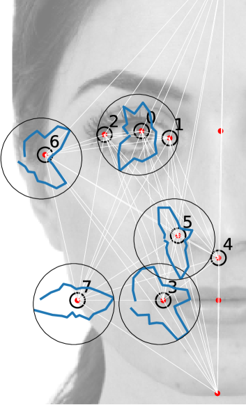
Figure 2.1: Facial landmarks $i=0,\ldots,7$ whose 2D coordinates ${\vec{r}}_{i}$ constitute the face space (signaled with black circles). Their position in the figure correspond to the average position, $\langle{\vec{r}}_{i}\rangle$. The background image corresponds to the texture degrees of freedom of the reference portrai, see [9]. The blue lines are polar hystograms ${\sf h}(\phi)$ (the radius is proportional to ${\sf h}(\phi)$) corresponding to the experimental distribution of angle landmark fluctuations around their average position.

The database consists in the set of landmark geometric coordinates ${\cal S}=\{{\bf r}^{(s)}\}_{s=1}^{S}$, where $s$ is the facial vector index corresponding to the $\cal N$ vectors sculpted by each of the ${n_{\rm s}}$ experimental subjects (hence: $S={n_{\rm s}}{\cal N}$). We will call ${\bf r}^{(s)}=(r^{(s)}_{({\sf x},1)},\ldots,r^{(s)}_{({\sf x},{n})},r^{(s)}_{({\sf y},1)},\ldots,r^{(s)}_{({\sf y},{n})})$ the vector whose $2{n}$ components are the $({\sf x},{\sf y})$ Cartesian coordinates of a set of ${n}=8$ landmarks, in units of the facial height. The landmarks (signaled with an empty circle in figure 6.2) are a subset of the set of landmarks used for the image deformation in the [9] experiment (signaled with red points in figure 6.2). We will also refer to the 2D Cartesian vector of the $i$-th landmark as ${\vec{r}}_{i}=({\sf x}_{i},{\sf y}_{i})$, and define the fluctuations of the landmark positions with respect to their average value as ${\vec{\Delta}}_{i}={\vec{r}}_{i}-\langle{\vec{r}}_{i}\rangle$, where $\langle\cdot\rangle$ denotes the experimental average, $\langle\cdot\rangle=(1/S)\sum_{s}\cdot$. An important aspect of the dataset is that even the coordinates of the restricted set of ${n}=8$ landmarks, ${\bf r}^{(s)}$, are redundant and depend on 10 coordinates only, due to the presence of $2{n}-10=6$ constraints that result from the very definition of the face-space. Such constraints are described in detail in the SI.

2.1 The Maximum Entropy models

We propose two probabilistic generative models of the set of selected faces, inferred from the dataset $\cal S$. They result form the Maximum Entropy (MaxEnt) method [17, 18, 19, 20], which provides the maximum entropy probability distribution $\cal L(\cdot|\bm{\theta})$ being consistent with the average experimental value of some observables of the data, $\langle{\Sigma}\rangle$, that will be called sufficient statistics. $\cal L$ must satisfy $\langle\Sigma\rangle_{\cal L}=\langle\Sigma\rangle$, where $\langle\cdot\rangle_{\cal L}$ refers to the theoretical average according to the distribution $\cal L$ (see a more precise definition in the SI). In the case of the Gaussian or 2-MaxEnt model, the sufficient statistics is given by the $2n$ averages $\langle\Delta_{\mu}\rangle$ and by the $2{n}\times 2{n}$ matrix of horizontal, vertical and oblique correlations among couples of vertical and horizontal landmark coordinates, whose components are $C_{\mu\nu}=\langle\Delta_{\mu}\Delta_{\nu}\rangle$. In these equations, the $2{n}$ Greek indices $\mu=i,{\sf c}_{i}$ denote the ${\sf c}_{i}={\sf x},{\sf y}$ coordinates of the $i$-th landmark. The 2-MaxEnt model probability distribution takes the form (see the SI) of a Maxwell-Boltzmann distribution, ${\cal L}({{\bm{\Delta}}}|\bm{\theta})=\frac{1}{Z}\exp\left(-H[{{\bm{\Delta}}}|\bm{\theta}]\right)$. In this equation, $Z$ is a normalising constant (the partition function, in the language of statistical physics) depending on $\bm{\theta}$, and $H=H_{2}$ (the Hamiltonian) is the function:

$$H_{2}[{{\bm{\Delta}}}|\bm{\theta}] = \frac{1}{2}{\bm{\Delta}}^{\dagger}\cdot J\cdot{\bm{\Delta}}+{\bf h}^{\dagger}\cdot{{\bm{\Delta}}}.$$ (2.1)

The model depends on the parameters $\bm{\theta}=\{J,{\bf h}\}$, or the $2{n}\times 2{n}$ matrix of effective interactions $J$ and the $2{n}$ vector of effective fields, $\bf h$. Due to the symmetry of matrix $J$, the number of independent parameters in the 2-MaxEnt model is $D+D(D+1)/2$, where $D=2{n}$ is the dimension of the vectors of landmark coordinates $\bm{\Delta}$. The value of these parameters is such that the equations $\langle{\bm{\Delta}}\rangle=\langle{\bm{\Delta}}\rangle_{\cal L}$ and $\langle\Delta_{\mu}\Delta_{\nu}\rangle_{\cal L}=C_{\mu\nu}$ are satisfied. This is equivalent to require that $\bm{\theta}$ are those that maximise the likelihood of the joint $\cal L$ over the database $\cal S$ (the Maximum Likelihood condition). The solution of such an inverse problem is (see SI): $J=C^{-1}$, ${\bf h}=J\cdot\langle{\bm{\Delta}}\rangle$, and $Z={(2\pi)^{n}}\exp({\bf h}^{\dagger}\cdot J^{-1}\cdot{\bf h}/2){(\det J)^{-1/2}}$, where the $-1$ power in equation $J=C^{-1}$ denotes the pseudo-inverse operation, or the inverse matrix disregarding the null eigenvalues induced by the database constraints (see SI).

We will define as well the non-linear, or 3-MaxEnt model. In this case, the sufficient statistics is given by averages, pairwise correlations and correlations among 3-landmark coordinates, $C^{(3)}_{\mu\nu\kappa}=\langle\Delta_{\mu}\Delta_{\nu}\Delta_{\kappa}\rangle$. The 3-MaxEnt model probability distribution ${\cal L}(\cdot|{\bf h},J,Q)$ assumes the Maxwell-Boltzmann form, with Hamiltonian $H=H_{2}+H_{3}$, where $H_{3}$ is:

$$H_{3}[{\vec{\bm{\Delta}}}|Q] = \frac{1}{6}\sum_{\mu\nu\kappa}\Delta_{\mu}\Delta_{\nu}\Delta_{\kappa}Q_{\mu\nu\kappa}$$ (2.2)

Besides ${\bf h}$ and $J$, the non-linear MaxEnt model depends on a further tensor of three-wise interaction constants among triplets of landmark coordinates. Consequently, the number of independent parameters is $D+D(D+1)/2+D(D-1)(D-2)/6$. The solution of the inverse problem for the non-linear MaxEnt model does not take a closed analytic form. The maximum likelihood value of the parameters $\bm{\theta}=({\bf h},J,Q)$ is numerically estimated by gradient ascent (see section 2 and the SI).

2.2 Learning in the non-linear models.

In the case of the 3-MaxEnt model, we have numerically the maximum likelihood value of the parameters $\bm{\theta}^{*}$ by means of deterministic gradient ascent, using an algorithm that will be presented in a dedicated publication. A detailed explanation of the learning protocol may be found in the SI. Before inferring the data with the non-linear models (3-MaxEnt and GRBM) we have eliminated a subset of redundant $6$ coordinates from the original $2{n}$ coordinates. The data has been standardised in order to favor the convergence of the likelihood maximisation.

2.3 The Restricted Boltzmann Machine model for unsupervised inference.

We have learned the data with the (Gaussian-Binary) Restricted Boltzmann Machine (GRBM) model of unsupervised inference [33, 34]. We have employed the open-source software [38] for the efficient learning of GRBM. The learning protocol and parameters are described in detail in the SI.

3 Results

We will now present an assessment of the description of the database according to the inference models described in the precedent section. In sec. 3.1 we will argue that the Harmonic MaxEnt model is a faithful representation of the dataset. Finally, in subsection 3.2, we will argue that the matrix of effective interactions $J$ provides meaningful information, beyond the raw information present in the raw experimental measure $C$.

3.1 Quality of the MaxEnt models as generative models

3.1.1 Histograms of single landmark-angle fluctuations

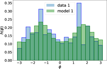
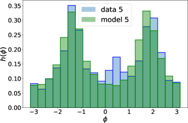
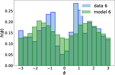
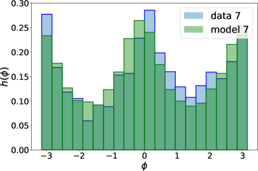
Figure 3.1: Experimental ${\sf h}^{(i)}(\phi)$ versus theoretical, ${\sf h}^{(i)}_{\sf t}(\phi)$ distributions of angle landmark fluctuations, for several landmarks, $i=1,5,6,7$, see fig. 6.2 (from left to right, from top to bottom).

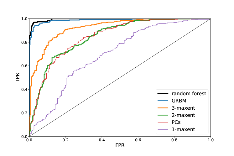
Figure 3.2: ROC curves corresponding to the geneder classification. Different curves correspond to different algorithms. PC’s refers to a $\sf t$-Student test of the difference in the principal components of a vector with respect to their average value in the $A$, $B$ sets.

The quality of the 2-MaxEnt generative model as a faithful description of the database may be evaluated by the extent to what the model ${\cal L}$ reproduces observables $O$ that it is not required to reproduce by construction. In other words, observables that cannot be written in terms of couples and triplets of coordinates $\Delta_{\alpha}$. The model is faithful in the extent to what $\langle O\rangle\simeq\langle O\rangle_{\cal L}$.

The $i$-th landmark coordinates $\vec{\Delta}_{i}$ tend to fluctuate in the database with respect their average position $\langle\vec{\Delta}_{i}\rangle=\vec{0}$. As a nonlinear observable $O$ we will consider the angle that the $i$-th landmark fluctuation $\vec{\Delta}_{i}$ forms with the $\sf x$-axis. This quantity will be referred to as $\phi_{i}^{(s)}=\arctan(\Delta_{i,{\sf y}}^{(s)}/\Delta_{i,{\sf x}}^{(s)})$. In figs. 6.2,3.1, we report the empirical histogram of angles, ${\sf h}(\phi_{i})$ for some landmarks $i$. Remarkably, some landmarks’ angle distribution exhibit local maxima, probably reflecting their tendency to follow the direction of some inter-landmark segments (as it is apparent for the $3$-rd and $6$-th landmark’s in figure 6.2). We have compared the empirical histograms with the theoretical $\phi_{i}$ distributions according to the model. These have been obtained as the angle histograms of a set of $S$ vectors $\bm{\Delta}$ sampled from the inferred distribution ${\cal L}(\cdot|\bm{\theta})$ (see fig. 3.1). The 2-MaxEnt model satisfactorily reproduces most of the landmark angle distributions. The empirical angle distribution, in other words, is reasonably well reproduced by the theoretical distribution ${\sf h_{t}}(\varphi)=\int{\rm d}{{\bm{\Delta}}}\,{\cal L}({\bm{\Delta}}|\bm{\theta})\delta(\phi({\bm{\Delta}})-\varphi)$. It is important to remark that the model-data agreement on ${\sf h}(\phi_{i})$ is observed also for large values of $\phi_{i}\in(-\pi/2,\pi/2)$ (see fig. 3.1), and not only for small values of $\phi_{i}$, for which it approximately becomes $\Delta_{i,{\sf y}}/\Delta_{i,{\sf x}}$ (whose average is related to the correlation $C_{\alpha\beta}$, see SI).

We conclude that, very remarkably, a highly non-linear observable as $\phi$ is well described by the 2-MaxEnt model, albeit it has been inferred from linear (pairwise) correlations only. In this sense, the 2-MaxEnt model is a faithful and economic description of the dataset. This picture is confirmed by the results of the following section which suggest, however, that a description of the gender differences in the dataset require taking into account effective interactions of order $p>2$.

3.1.2 Performance of the MaxEnt model in a classification task

We now further evaluate the quality of the 2- and 3-MaxEnt models by assessing their efficiency to classify a test database of vectors in two disjoint subsets ${\cal S}={\cal S}_{A}\cup{\cal S}_{B}$ corresponding to the gender of the subject that sculpted the facial vector in [9]. We compare such efficiency with that of the GRBM model of ANN (see [33, 34], sec. 2 and the SI). This comparison allows to assess the relative relevance of products of $p$-facial coordinates $\Delta_{\alpha}$ in the classification task: averages ($p=1$), pairwise correlations ($p=2$), and non-linear correlations of higher, $p>2$ order (modelled by the 3-MaxEnt and GRBM models only).

The dataset is divided in two disjoint classes ${\cal S}_{A},{\cal S}_{B}$. Afterwards, both ${\cal S}_{A,B}$ are divided in training- and test- sets ($20\%$ and $80\%$ of the elements of ${\cal S}_{A,B}$, respectively), and inferred the $A$ and $B$ training sets separately, with the MaxEnt and GRBM models. This results in six ($\{2,3,G\}\times\{A,B\}$) sets of parameters $\bm{\theta}^{2,3,G}_{A,B}$, where the super-index refers to the model. Given a vector ${\bm{\Delta}}$ belonging to the $A$ or $B$ test set, the score ${\sf s}({\bm{\Delta}})=\ln{\cal L}({\bm{\Delta}}|\bm{\theta}_{A})-\ln{\cal L}({\bm{\Delta}}|\bm{\theta}_{B})$ is taken as the estimation of the model prediction for $\Delta\in{\cal S}_{A}$. The resulting Receiver Operating Characteristic (ROC) curves [35] are shown in fig. 3.2 for the various models considered.

Considering only the averages $\langle{\bm{\Delta}}\rangle$ as sufficient statistics (or, equivalently, inferring only the fields $\bf h$ (and setting $J_{ij}=\sigma^{-2}_{i}\delta_{ij}$ in equation 2.1) results in a poor, near-casual classification (specially in the most interesting region of the ROC curve, for small ${\rm FPR}$ and large ${\rm TPR}$), see figure 3.2. The 2-MaxEnt model allows, indeed, for a more efficient classification. Rather remarkably, the 3-MaxEnt and GRBM models gradually improves the classification. We interpret this as an indication of the fact that non-linear effective interactions at least of fourth order are necessary for a complete description of the database. For completeness, we have included a comparison with the Random Forest (RF) algorithm [35]. As shown in fig. 3.2, RF achieves the highest classification accuracy (auROC$=0.995$, see SI). We notice that this does not imply that the unsupervised models are less accurate: the RF algorithm is advantaged, being a specific model trained to classify at best the $A,B$ partitions, not to provide a generative model of the $A$ and $B$ partitions separately.

We report the maximal accuracy scores for all the algorithms: RF ($0.971$); GRBM ($0.952$); 3-MaxEnt ($0.865$); 2-MaxEnt ($0.764$); 1-MaxEnt ($0.680$). The 2-MaxEnt model efficiency is, as expected, compatible with that of a $\sf t$-Student test regarding the differences in the principal component values of $A$ and $B$ vectors, see fig. 3.2. See the auROC scores of all the algorithms in the SI.

We conclude that, on the one hand, the subjects’ gender strikingly determines her/his preferred set of faces, to such an extent that it may be predicted from the sculpted facial modification with an impressively high accuracy score [35]: a $97.1\%$ of correct classifications. On the other hand, the relative efficiency of various models highlights the necessity of non-linear interactions for a description of the differences among male and female facial preference criterion in the database. Arguably, such nonlinear functions play also a role in the cognitive process of facial perception. The criterion with which the subjects evaluate and discriminate facial images seems to involve not only proportions $r_{\alpha}/r_{\beta}$ (related to the pairwise correlations $C_{\alpha\beta}$, see SI), but also triplets and quadruplets of facial coordinates influencing each other (yet, see the SI for an alternative explanation).

3.2 Analysis of the matrix of effective interactions

We now show that the generative models may provide directly interpretable information. This is an advantage of the MaxEnt method, whose parameters, the effective interaction constants, may exhibit an interpretable significance.

The 2-MaxEnt model admits an immediate interpretation. The associated probability density ${\cal L}({{\bm{\Delta}}}|\bm{\theta})=\exp\left(-H_{2}[{{\bm{\Delta}}}|\bm{\theta}]\right)/Z$ formally coincides with a Maxwell-Boltzmann probability distribution of a set of ${n}$ interacting particles in the plane (with positions $\vec{\Delta}_{i}$, $i=1,\ldots,n$), subject to the influence of a thermal bath at constant temperature. Each couple $i$,$j$ of such fictitious set of particles interacts through an harmonic coupling that corresponds to a set of three effective, virtual springs with non-isotropic elastic constants, ${J^{({\sf x}{\sf x})}}_{ij},{J^{({\sf y}{\sf y})}}_{ij},{J^{({\sf x}{\sf y})}}_{ij}$ corresponding (see equation 2.1) to horizontal, vertical and oblique displacements, $\Delta_{i,{\sf x}}-\Delta_{j,{\sf x}}$, $\Delta_{i,{\sf y}}-\Delta_{j,{\sf y}}$, and $\Delta_{i,{\sf x}}-\Delta_{j,{\sf y}}$, respectively.

The inferred effective interactions are more easily interpretable if one considers, rather than their ${\sf x}{\sf x}$, ${\sf y}{\sf y}$ and ${\sf x}{\sf y}$ components, the longitudinal and torsion effective interactions, $J_{ij}^{\parallel}$ and $J_{ij}^{\perp}$, respectively. The longitudinal coupling $|J_{ij}^{\parallel}|$ may be understood (see the SI for a precise definition) as the elastic constant corresponding to the virtual spring that anchors the inter-$ij$ landmark distance to its average value, $\langle r_{ij}\rangle$ (where $\vec{r}_{ij}=\vec{r}_{j}-\vec{r}_{i}$). In its turn, the torsion interaction $|J_{ij}^{\perp}|$ is the elastic constant related to fluctuations of $\vec{r}_{ij}$ along the direction normal to $\vec{r}_{ij}$ or, equivalently, to fluctuations of the $ij$-segment angle, with respect to its average value that we will call $\alpha_{ij}=\arctan(\langle r_{ij,{\sf y}}\rangle/\langle r_{ij,{\sf x}}\rangle)$.

In fig. 3.3-A,B we show the quantities $|J_{ij}^{\parallel}|$ and $|J_{ij}^{\perp}|$ for those couples $i,j$ presenting a statistically significant value (for which the $\sf t-$value $t_{ij}=|J_{ij}|/\sigma_{J_{ij}}>1$, see sec. 2). The width of the colored arrow over the $i,j$ segment is proportional to $|J_{ij}^{\parallel}|$ (blue arrows in fig. 3.3-A) and $|J_{ij}^{\perp}|$ (red arrows in fig. 3.3-B). We notice that there exist inter-landmark segments for which $|J_{ij}^{\parallel}|$ is significant while $|J_{ij}^{\perp}|$ is not (as the $0,4$ or the $5,6$ segments) and vice-versa (as the $6,7$ and $2,5$). This suggests that $|J_{ij}^{\parallel}|$, $|J_{ij}^{\perp}|$ actually capture the cognitive relative relevance of distance fluctuations around $\langle r_{ij}\rangle$, and of angle fluctuations around $\alpha_{ij}$.

In the SI we explain in more detail the analogy with the system of particles. We also analyse the dependence of the torsion and longitudinal effective interactions, $|J_{ij}^{\parallel}|$ and $|J_{ij}^{\perp}|$, with the average distance and angle of the $ij$ inter-landmark segment, showing that there is a moderate decreasing trend of $|J_{ij}^{\parallel}|$ with $\langle r_{ij}\rangle$

We remark that the prominent importance of the inter-segment angles $ij$ highlighted in fig. 3.3-B is fully compatible with the analysis presented in ref. [9] at the level of the oblique correlation matrix ${C^{({\sf x}{\sf y})}}$, and it goes beyond, as far as it quantitatively assess their relative relevance. As we will see before, such information cannot be retrieved from the experimental matrix $C$ only.

3.2.1 Extra information retrieved with effective interactions

A relevant question is to what extent the inferred effective interactions $J$ provide interpretable information, inaccessible from the raw experimental correlations $C$. In the general case, couples of variables may be statistically correlated through spurious correlations, even in the absence of a causal relation among them (see the SI). In the present case, the main source of spurious correlations is the presence of the constraints among various landmark coordinates. The MaxEnt inference eventually subtracts (through the pseudo-inverse operation) the influence of the constraints from matrix $J$, which describes the essential effective mutual influence among pairs of coordinates of prominent relative importance (see the SI).

The differences among $C$ and $J$ matrices are shown in fig. 3.3-C, where the arrows represent the absolute value of the raw experimental matrix elements $C^{\parallel}_{ij}$. Remarkably, all but two of the matrix elements result statistically significant ($t$-value $>1$): matrix $C^{\parallel}$ can be hardly used to assess the relative relevance of various inter-landmark segments. The effective interaction matrix $J$ disambiguates the correlations propagated by the constraints, attributing them to the effect of a reduced set of elastic constants, in the particle analogy. Such attribution is not unambiguous, but the result of an inference procedure.

An in-depth comparison among $C$ and $J$ is presented in the SI, where we consider also the alternative method of avoiding the constraints, consisting in inferring from a non-redundant set of coordinates. We conclude that, in the general case, and for the sake of the interpretation of the effective interactions, it may convenient to infer from a database of redundant variables, eliminating a posteriori the influence of the null modes associated to the constraints, or the $C$-eigenvectors associated to non-linear constraints.

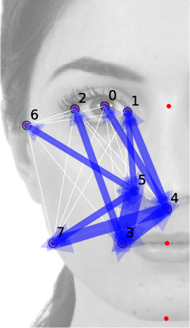
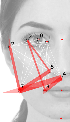
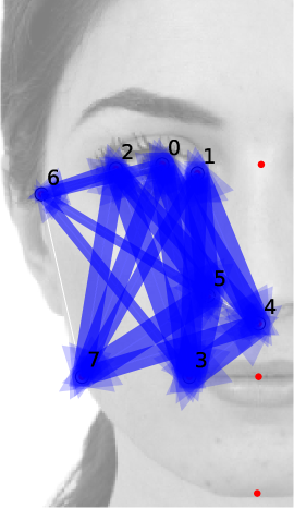
Figure 3.3: Modulus of the matrices $J^{\parallel}$ (left), $J^{\perp}$ (center), $C^{\parallel}$ (right). The width of the arrow joining the $i$-th and $j$-th landmarks is proportional to $|A_{ij}|$, where $A$ is the corresponding matrix. Only significant matrix elements have been plotted: only those exhibiting a $t\sf$-value larger than one: $t_{ij}=|A_{ij}|/\sigma_{A_{ij}}>1$.

4 Discussion

We have presented an application of the Maximum Entropy (MaxEnt) method to the inference of a database of preferred facial modifications. Much work has been devoted to the supervised inference of the rating assigned to a set of face-space vectors –a technological, more than scientific aim. Nevertheless, such studies indirectly allow for an assessment of the relative impact of various facial traits on perceived beauty [6]. These remain, along with the nature of inter-subject differences in preferred faces, controversial questions. As a further tool to address them, we here propose an alternative inference scheme in which the variability to be inferred is not the average rating assigned to different natural faces, but the inter-subject variability of preferred modifications in a subspace of the face-space.

To our knowledge, the present work is the first unsupervised inference approach in facial preference research. It presents at least three innovative, distinguishing traits: the inference is performed over a set of preferred facial modifications, each one corresponding to a different subject; it avoids the use of ratings, a limited quantity [6, 9], and the curse of dimensionality associated to the rating of natural faces; it accounts for the mutual influence of couples and $p-$plets of facial features, $p>2$, hence beyond a principal component analysis. At the same time, the inference is done in terms of interpretable quantities involving “physical” facial coordinates only, hence overcoming the black-box issue.

The present approach allows to clarify several aspects regarding facial preference. First, that the cognitive mechanisms related to facial discrimination in the brain definitely involves the mutual influence of couples of landmarks, more than the positions of single landmarks. Moreover, the results suggest as well that non-linear operators of the facial coordinates are involved in the cognitive process (see secs. 3.1.1,6.16). The recent de-codification of the neural code for facial recognition in the primate brain [36] has revealed that recognition is based on linear operations (or projections in the geometric and texture principal axes) in the face-space. The evaluation of attractiveness (probably related to the higher-level inference of abstract personality attributes [11, 12, 7, 14, 15, 1, 16]) may be a more complex process, requiring the evaluation of non-linear operations in the face-space.

Second, and rather remarkably, the introduction non-linear effective interactions allows for an astonishingly high classification efficiency of the facial vectors according the subject’s gender: a $97.1\%$ of correct classifications, for the random forest algorithm. This implies that the subject’s gender strikingly determines her/his facial preference criteria. Our results strongly suggest that such an influence is not reflected in differences in the position of single landmarks. Moreover, the MaxEnt method provides the set of proportions (see fig. 3.3) and triplets of landmarks which male and female subjects tend to evaluate more differently.

In summary, the MaxEnt method provides a faithful probabilistic generative model of the database of preferred facial variations of ref. [9], describing the inter-subject fluctuations around of the preferred facial vector (given a reference background portrait). We demonstrate that such fluctuations encode, and may accurately reveal, meaningful information regarding the subject that selected the facial vector, such as her/his gender. As also suggested by the multiple motive hypothesis, many other subjects’ attributes and distinguishing traits may influence her/his personal preferences in the face-space and, hence, could be retrieved from their sculpted facial vectors. By sculpting a set of preferred facial modifications the subject reveals a large amount of information, arguably more than the rating of natural images would do.

According to this idea, the analysis of a subjects’ sculpted facial vectors could be used for an assessment, on a voluntary basis, of her/his abstract personality dimensions most influencing attractiveness, as the subjects’ “traits of desired personality” [37]. In the same way, and as far as the complete subjectivity picture proposed in [9] is valid, an accurate enough experiment of preferred variation sculpture could be used as a voluntary fingerprint identity test.

Furthermore, the present study represents a novel case of study for the application of the MaxEnt method for unsupervised inference, in particular for the assessment of the relevant order of interaction by comparison with an ANN model and for the comparison among various strategies of inference in the presence of constraints.

Possible extensions of this work are the generalisation to different datasets and facial codification methods (see the SI for a discussion on the generality of the present approach); the classification of different subject’s features from her/his set of sculpted faces; the analysis of medical imaging data characterised by the 3D position of landmark points.

5 Acknowledgements

We acknowledge Andrea Gabrielli, Irene Giardina, Carlo Lucibello, Giorgio Parisi and Massimiliano Viale for inspiring discussions. Particular thanks to Andrea Cavagna for his suggestions and comments to the draft.

6 Supplementary Information

6.1 Introduction to the Maximum Entropy principle: Correlations vs effective interactions

Consider an $n$-dimensional space of vectors, ${\bf x}=(x_{i})_{i=1}^{n}\in\chi$, along with a set of $K$ observables, $O_{k}:\chi\to\mathbb{R}$, $k=1,\ldots,K$. The maximum entropy approach [17, 18, 19, 20] provides the most probable probability distribution $P({\bf x}|{\bm{\lambda}})$, ${\bf x}\in\chi$, which is consistent with a fixed value of the operators, in the sense that their average according to $P$, $\langle O_{k}\rangle_{P}$ is constraint to assume a fixed value,

$$\langle O_{k}\rangle_{P}=o_{k}$$ (6.1)

(where $\langle O_{k}\rangle_{P}=\int{\rm d}{\bf x}\,O_{k}({\bf x})P({\bf x}|{\bm{\lambda}})$). In other words the maximum entropy probability distribution $P_{\rm me}$ is the one exhibiting highest entropy (i.e., the most random, or less structured distribution) subject to the constraint (6.1), and to no other constraint. It assumes the form:

$$P_{\rm me}({\bf x})=\frac{1}{Z({\bm{\lambda}})}\exp\left[\sum_{k=1}^{K}\lambda_{k}O_{k}({\bf x})\right]$$ (6.2)

$Z({\bm{\lambda}})$ being a normalizing constant. The maximum entropy probability distribution is, hence, formally identical to a Maxwell-Boltzmann distribution in the canonical ensemble at temperature $=1$, with effective Hamiltonian ${\cal H}=-\sum_{k}\lambda_{k}O_{k}$. It is important to remark that no assumption at all has been done about thermal equilibrium, ergodicity, nor about the existence of an effective interaction in energy units: the Maxwell-Boltzmann form is a consequence of the maximum entropy assumption –reflecting, rather, absence of hypothesis– of a probability distribution subject to constraints on the average of some operators. The values of the Lagrange multipliers $\lambda$’s in (6.2) are such that the constraints in (6.1) are satisfied.

In the context of unsupervised statistical inference, one infers from a finite number $M$ of experimental measures of the observables $O_{k}$, to which correspond the values $o_{k}^{(m)}$, $m=1,\ldots,M$. The maximum entropy distribution provides a generative probabilistic model for the data, that is aimed to be a faithful representation of the experimental dataset and, at the same time, a generalisation of the dataset, not too dependent on the specific realisation of the database that is being inferred. For this reason, $P$ is chosen to reproduce the experimental value of a limited set of observables, depending on the dataset. Ideally, a faithful and general model should be consistent with the minimum set of experimental averages that allow to reproduce some essential database properties and, at the same time, that may be significantly inferred given the database finiteness. Once the observables have been selected, a possible choice for their value $o_{k}$ (determining the value of the parameters $\lambda_{k}$) in 6.1 is the experimental average, $\langle O_{k}\rangle=(1/M)\sum_{m=1}^{M}o_{k}^{(m)}$. This choice $o_{k}=\langle O_{k}\rangle$ is equivalent to the Maximum Likelihood prescription of the whole experimental database:

$$\{\lambda^{*}_{k}\}_{k}=\arg\max_{\{\lambda_{k}\}_{k}}\sum_{m=1}^{M}\ln P({\bf x}^{(m)}|{\bm{\lambda}})$$ (6.3)

where ${\bf x}^{(m)}$ is the $m$-th experimental configuration, and $o^{(m)}_{k}=O_{k}({\bf x}^{(m)})$. The parameters $\lambda$ are called effective interactions, in the language of statistical physics. In the case that the observables to be reproduced by $P$ are the data correlations of order $n\leq p$ (where the correlations of order $n$ are defined as $C^{(n)}_{i_{1},\cdots,i_{n}}=\langle x_{i_{1}}\cdots x_{i_{n}}\rangle$), the effective interactions assume the form of $n$-th order tensors $J^{(n)}$ coupling $n$-plets of vector coordinates, with $n=1,\ldots,p$.

A self-consistency criterion for the choice of the sufficient statistics $O_{k}$ is that of calculating different nontrivial observables according to $P$ (different from the sufficient statistics, i.e., observables that $P$ is not required to reproduce by construction, and that cannot be expressed in terms of the sufficient statistics), and comparing them with their experimental counterparts. In particular, a criterion is that of choosing the $n\leq p$-th order correlations as sufficient statistics, with $p$ being the minimum value such that the $p+1$-th order experimental correlations are satisfactorily reproduced by $P_{\rm me}$ (i.e., $\langle x_{i_{1}}\cdots x_{i_{p+1}}\rangle\simeq\langle x_{i_{1}}\cdots x_{i_{p+1}}\rangle_{P}$), and such that all the parameters corresponding to such sufficient statistics may be significantly inferred from the data.

Correlations and effective interactions. The effective interaction tensors $J^{(n)}$ may admit, in certain circumstances, an interpretation regarding the mutual effective influence among variables, beyond the statistical correlation among them (whose experimental value is $C^{(n)}$). Correlations and effective interactions are actually different. Focusing for simplicity in $p=2$, the pairwise correlations are but the statistical consequence of the effective interactions among couples of landmarks causing them. This is the case in the direct problem (the calculation of $C^{(2)}$ from $J^{(2)}$): in this case, it may happen that the matrix $J^{(2)}$ is sparser than $C^{(2)}$: there are couples of variables not influencing each other that, nevertheless, result statistically correlated. In the direct problem, the Maximum Entropy method may allow for a discrimination of the spurious correlations of couples of components that are correlated although they do not influence each other (but are, instead, commonly and mutually influenced by other components). This a frequent phenomenon in biological data [22, 39], with an obvious interpretation in statistical physical terms: in the general case, the mutual influence among a sparse set of couples of bodies propagates statistically, leading to emergent, collective phenomena. A paradigmatic and extreme case of this general phenomenology is critical behaviour [40], in which microscopic interactions lead to macroscopic correlations: long-range and high-order body correlations originate from short-range, sparse and pairwise interactions [22]).

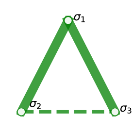
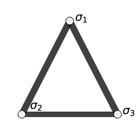
Figure 6.1: Effective interactions (left) versus the emerging statistical correlations (right) among three binary variables, $\sigma_{i}=\pm 1$, $i=1,2,3$. The effective interactions are given by the symmetric matrix $J_{12}=J_{13}=2$, $J_{23}=-3/4$ (i.e., 2,3 are negatively coupled). The correlations $\langle\sigma_{i}\sigma_{j}\rangle$ are given by their expectation value according to the Maxwell-Boltzmann probability distribution corresponding to a pairwise interaction given by matrix $J$: $\langle\sigma_{i}\sigma_{j}\rangle=\sum_{\bm{\sigma}}\sigma_{i}\sigma_{j}P({\bm{\sigma}})$, with $P({\bm{\sigma}})=\exp(+\sum_{i<j}\sigma_{i}\sigma_{j}J_{ij})/Z$ where $Z=\sum_{\bm{\sigma}}\exp(+\sum_{i<j}\sigma_{i}\sigma_{j}J_{ij})$. The line width is proportional to the absolute value $|A_{ij}|$ of the corresponding matrix element. The dashed line in the $J$ triangle indicates that $J_{23}$ is negative (i.e., there is a tendency of $2$ to decrease when $3$ increases and vice-versa). Such tendency is, however, not reflected in the correlation matrix, which presents all positive elements.

Probably the simplest illustration of the emergence of spurious statistical correlations is that of three variables ($x_{1},x_{2},x_{3}$ in fig. 6.1, of which only two of them are strongly interacting (in the figure $J_{12}=J_{13}=2$), while the second and third are moderately interacting (or even negatively interacting, as in the figure: $J_{23}=-1$). Such an information is not accessible from the emerging correlations $\langle x_{i}x_{j}\rangle_{P(\cdot|J)}$ (in the direct problem), revealing a strong, positive correlation among all the variables. Conversely, in the inverse problem (i.e., when an empirical correlation matrix is given, resulting from an average of a sufficiently high number of measures), the Maximum Entropy method may provide not only a generative model, $P(\cdot|J_{*}^{(n)})$, but also the most probable interaction matrices $J_{*}^{(n)}$ suggesting that, indeed, the correlation among $2$ and $3$ is (most likely, given the data and the sufficient statistics, and within the Maximum Likelihood hypothesis) a statistical consequence of the mutual influences of $1,2$ and of $1,3$. This information is not unambiguously elicited from the data, but the result of an inference procedure: the most probable guess given the inference model and the ambiguity induced by the data finiteness.

6.2 Maximum Entropy inference from pairwise correlations with a priori constraints

In this section we solve the problem of the Maximum Entropy (MaxEnt) inference from pairwise correlations (i.e., $p=2$), in the presence of linear constraints involving the coordinates.

In the absence of constraints, the Maximum Likelihood solution to the problem, equation (6.3) is analytic and straightforward. Suppose that one infers from a database composed by $S$ experimental realisations $\{{\bf x}^{(s)}\}_{s=1}^{S}$ of a real, $D$-dimensional vector, ${\bf x}=(x_{i})_{i=1}^{D}\in\mathbb{R}^{D}$. The sufficient statistics to infer from is by hypothesis the correlation matrix (supposing null-average vectors): $C_{ij}=\langle x_{i}x_{j}\rangle$ where $\langle\cdot\rangle$ represents, as before, the experimental average: a symmetric, positive definite matrix. The MaxEnt probability distribution is, consequently, the multi-variate normal distribution:

$${P}({\bf x}|J)=\left[\frac{\det J}{(2\pi)^{n}}\right]^{1/2}\exp[-\frac{1}{2}{\bf x}^{\dagger}J{\bf x}].$$ (6.4)

The Maximum Likelihood solution for the matrix $J$, $J^{*}$, is that satisfying that the theoretical pairwise correlations $\langle x_{i}x_{j}\rangle_{P}={J^{-1}}_{ij}$ coincide with the experimental correlations $C_{ij}$. This is satisfied whenever $J^{*}=C^{-1}$.

We now consider the presence of linear constraints involving the coordinates, $x_{i}$. Each linear constraint may be expressed in the form ${\bm{a}}_{j}^{\dagger}{\bf x}=c_{j}$, being ${\bm{a}}_{j}$ a real $D$-dimensional vector and $c_{j}$ a real constant, for the $j$-th constraint. If all the vectors in the database $\{{\bf x}^{(s)}\}_{s=1}^{S}$, are subject to the constraints, each constraint induces a null mode (a zero eigenvalue) in the experimental covariance matrix. In this case, the Maximum Likelihood solution to the problem, i.e., the probability distribution $P(\cdot|J)$ such that $\langle x_{i}x_{j}\rangle_{P}=C_{ij}$ cannot simply be $J^{*}=C^{-1}$, since matrix $C$ actually exhibits a vanishing determinant.

We will see that Maximum Likelihood solution in this case is $J^{*}=C^{-1}$, where the $-1$ exponent means the pseudo-inverse operation, a generalisation of the matrix inverse operation in which the null eigenvalues are avoided. We define the pseudo-inverse of the real, square matrix $A$ as:

$${A^{-1}}_{ij}=\sum_{k|\epsilon_{k}\neq 0}\epsilon_{k}^{-1}\eta^{(k)}_{i}\eta^{(k)}_{j}$$ (6.5)

where $\epsilon_{k}$, $\eta^{(k)}_{j}$ are the $k$-th eigenvalue and the $j$-th component of the $k$-th eigenvector of $A$, respectively.

We first consider the solution of the direct problem, $\langle x_{i}x_{j}\rangle_{P}$ from $J$, in a situation in which the interaction matrix $J$ is such that ${\rm rank}(J)=r<D$. In other words, $J$ exhibits $D-r$ null eigenvalues. Suppose that the eigenvalues $\lambda_{j}$ of $J$ are ordered in decreasing order, so that $\lambda_{j}=0$ for $j=r+1,\ldots,D$. In this case, the probability distribution $P({\bf x})$ in equation 6.4 is, trivially, constantly zero since the determinant of matrix $J$ vanishes. However, we can define a real function in the space of the $D$-dimensional variables ${\bf x}$:

$$\tilde{P}({\bf x})=\frac{1}{\tilde{Z}}\exp[-{\bf x}^{\dagger}J{\bf x}]\\$$ (6.6)

where $\tilde{Z}$ is a normalising factor involving the non-zero eigenvalues of $J$ only:

$$\tilde{Z}=\left[\frac{\tilde{\det}J}{(2\pi)^{r}}\right]^{1/2}\qquad\tilde{\det}J=\prod_{k=1}^{r}\lambda_{k}$$ (6.7)

The function $\tilde{P}$ may be considered as a normalised probability distribution, but only over the $r$-dimensional subspace of ${\mathbb{R}}^{D}$ expanded by the first $r$ eigenvectors of $J$: ${\mathbb{S}}_{+}={\rm span}\{{\bf e}^{(k)}\}_{k=1}^{r}$ with $1\leq k\leq r$. In other words, $\tilde{P}$ is a probability distribution on the subspace of ${\mathbb{R}}^{D}$, ${\mathbb{S}}_{+}$, defined by the vectors that are already subject to the constraints, for any value $c_{j}$’s of the constants associated to the constraints.

One can easily define a proper, normalised probability distribution $P$ defined in ${\mathbb{R}}^{D}$, by regularising the null modes associated to the constraints:

$$P({\bf x})={\tilde{P}}({\bf x})\prod_{j=r+1}^{D}\delta(x^{\prime}_{j}-{\sf c}_{j})$$ (6.8)

where the $D-r$-dimensional vector $(x^{\prime}_{r+1},\ldots,x^{\prime}_{D})$ is a vector of the projection of ${\bf x}$ in a basis of vectors expanding the space of the constraints (as the vectors ${\bf a}_{j}$ defining the constraints, before, $x^{\prime}_{j+r}={\bf a}_{j}^{\dagger}{\bf x}$). On the other hand, we define the $r$-dimensional vector ${\bf x}^{\prime}=(x^{\prime}_{1},\ldots,x^{\prime}_{r})$ as the projection of ${\bf x}$ over the first $r$ eigenvectors of $J$ (associated to a non-null eigenvalue): ${\bf x}^{\prime}=E{\bf x}$, where $E$ is the $r\times D$ matrix defined as the row-disposed eigenvectors, $E_{ij}=e^{(i)}_{j}$.

To each of the null eigenvalues corresponding to a constraint ${\bf a}\cdot{\bf x}=c$, is associated an invariance of ${\tilde{P}}$ with respect to the linear operator $G(c)$ that changes the value of the constraint, i.e., such that ${\bf a}\cdot(G(c){\bf x})=c$:

$${\tilde{P}}({\bf x}|J)={\tilde{P}}(G(c){\bf x}|J).$$ (6.9)

Indeed, $G$ acts on the subspace ${\mathbb{S}}_{0}$ only, while it is the identity in the subspace ${\mathbb{S}}_{+}$ (where ${\mathbb{S}}_{0}$ is defined as the complement of $\mathbb{S}_{+}$, i.e., $\mathbb{R}^{D}={\mathbb{S}_{+}}\times{\mathbb{S}}_{0}$). In the physical language, each eigenvector corresponding to a constraint is called a null mode, and represents a symmetry reflected in the invariance of the function ${\tilde{P}}$ with respect to the symmetry. The function $P$, in its turn, represents vectors for which the symmetry is broken, as the value of the constraint has been fixed. For example, if the vectors are constrained to have a constant sum of its components, $\sum_{i=1}^{D}x_{i}=c$, the corresponding eigenvector, or null mode ${\bf e}$, has all its components equal to $e_{i}=D^{-1/2}$. Consequently, the function ${\tilde{P}}$ is invariant under scale transformations.

We are now interested in the calculation of a general $n$-order cumulant $\langle\langle x_{s_{1}}\cdots x_{s_{n}}\rangle\rangle_{P}$ according to the distribution $P$ in (6.8), with $s_{j}=1,\ldots,D$. As it can be seen immediately, the $n$-th order cumulant is related to the $n$-th order derivative of the generating function through the standard cumulant expansion equation:

$$\langle\langle x_{s_{1}}x_{s_{2}}...x_{s_{n}}\rangle\rangle_{P}=\left.\frac{\partial^{n}\ln\tilde{Z}[{\bf h}^{\prime}]}{\partial h^{\prime}_{s_{1}}\partial h^{\prime}_{s_{2}}...\partial h^{\prime}_{s_{n}}}\right|_{{\bf h}={\bf 0}}$$ (6.10)

where the generating function $\tilde{Z}[{\bf h}]$ has the form:

$$\tilde{Z}[{\bf h}]=\left[\prod_{k=1}^{r}\int_{-\infty}^{+\infty}dz^{\prime}_{k}\right]e^{-\frac{1}{2}{\bf x}^{\dagger}J{\bf x}+{\bf h}^{\dagger}{\bf x}}$$ (6.11)

We notice that $\tilde{Z}[{\bf 0}]=\tilde{Z}$. We would like an analytical expression for $\tilde{Z}[{\bf h}]$. Using the relations ${\bf x}^{\prime}=E{\bf x}$ and $J=E^{\dagger}\Lambda E$, where $\Lambda$ is the $r\times r$ diagonal matrix whose diagonal is $\lambda_{1},\ldots,\lambda_{r}$, one obtains:

$$\tilde{Z}[{\bf h}]=\prod_{k=1}^{r}\int_{-\infty}^{+\infty}dx^{\prime}_{k}\exp\left[{-\frac{1}{2}{x^{\prime}}_{k}^{2}\lambda_{k}+x^{\prime}_{k}h^{\prime}_{k}}\right]$$ (6.12)

where ${\bf h}^{\prime}=E{\bf h}$. Using Gaussian integration rules, one finds:

$$\tilde{Z}[{\bf h}]=\tilde{Z}e^{\frac{1}{2}{\bf h}^{\dagger}J^{-1}{\bf h}}$$ (6.13)

where $J^{-1}$ is the pseudo-inverse of matrix $J$, ${J^{-1}}_{ij}=\sum_{k\leq r}\lambda_{k}^{-1}e^{(k)}_{i}e^{(k)}_{j}$. This equation is the generalisation of the standard expression for the generating function of the multi-variate normal distribution, to the case in which matrix $J$ is be non-invertible. As it is evident from the expression of $\tilde{Z}[{\bf h}]$ and from the cumulant expansion (6.10), and as it happens with the normal distribution, the only non-zero cumulant is the second-order cumulant $\langle\langle x_{i}x_{j}\rangle\rangle_{P}$, equal to the correlation $\langle x_{i}x_{j}\rangle_{P}$ in the case of null-averaged vectors. Its form is, from equation 6.10:

$$\langle x_{i}x_{j}\rangle_{P}={J^{-1}}_{ij}$$ (6.14)

where $J^{-1}$ is the pseudo-inverse of matrix $J$.

The theoretical correlation matrix whose elements are $\langle x_{i}x_{j}\rangle_{P}$ exhibits, as matrix $J$ does, rank equal to $r$. Hence, the theoretical correlation matrix $M_{ij}=\langle x_{i}x_{j}\rangle$ as a function of $J$ (i.e., the direct problem) is $M=J^{-1}$. Consequently, the $J^{*}$ that is needed to satisfy $C_{ij}=\langle x_{i}x_{j}\rangle_{P}$ given an experimental correlation matrix $C$ (i.e., the inverse problem) is $J^{*}=C^{-1}$, where the $-1$ power means the pseudo-inverse operation.

6.3 Constraints in the database of facial modifications

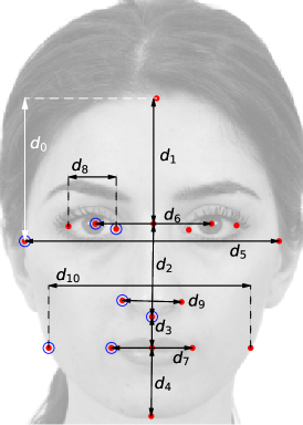
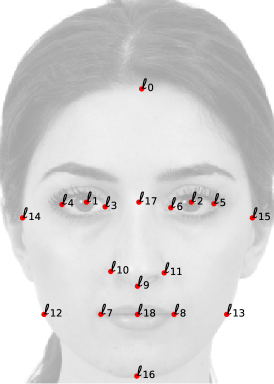
Figure 6.2: Left: definition of the face space in terms of inter-landmark distances $\bf d$. The landmark coordinates are, instead, the ${\sf x},{\sf y}$ 2D coordinates ${\vec{r}}_{i}$ of a subset of seven landmarks, marked with blue circles. Right: all the landmarks used for the facial deformation algorithm described in [9].

As we have explained in the main text, the facial modifications in the 2017 experiment are defined in terms of a set of 17 2D landmarks which are redundant in the sense that the positions of some of them may be deduced in terms of 10 coordinates only. The facial landmarks are, in particular, symmetric by construction, and hence the coordinates of the right-side landmark are determined given those of the left side. We have, hence, considered a subset of ${n}=8$ landmarks only (see figure 6.2 Furthermore, the landmark coordinates $r_{{\sf c},i}$ (where ${\sf c={\sf x},{\sf y}}$) in the database ${\cal S}$ are still subject to 6 constraints: indeed, $2\times{n}-6=10$, the numer of degrees of freedom. For instance, the nose endpoint abscissa is constrained to lie in the center of the image, $\Delta_{{\sf x},9}=0$, and the jaw landmark is defined to be at the same heigth of the mouth, $\Delta_{{\sf y},3}=\Delta_{{\sf y},7}$. We have intentionally kept such redundant information in the inferred training database. Indeed, the redundant information turns to be necessary for the correct interpretation of the inference parameters, as we will see in section 6.8.

The database ${\cal S}=\{{\bm{\Delta}}^{(s)}\}_{s=1}^{S}$ of facial displacements is, hence, highly constrained in the various facial coordinates. The following constraints hold, for all the vectors in the database:

$$\Delta_{4,{\sf x}} = 0$$ (6.15)

$$\Delta_{4,{\sf y}}-\Delta_{5,{\sf y}} = {\rm constant}$$ (6.16)

$$\Delta_{7,{\sf y}}-\Delta_{3,{\sf y}} = 0$$ (6.17)

$$\frac{\Delta_{0,{\sf y}}-\Delta_{1,{\sf y}}}{\Delta_{0,{\sf x}}-\Delta_{1,{\sf x}}} = {\rm constant}$$ (6.18)

$$\frac{\Delta_{0,{\sf y}}-\Delta_{2,{\sf y}}}{\Delta_{0,{\sf x}}-\Delta_{2,{\sf x}}} = {\rm constant}$$ (6.19)

$$\frac{\Delta_{1,{\sf x}}-\Delta_{0,{\sf x}}}{\Delta_{0,{\sf x}}-\Delta_{2,{\sf x}}} = {\rm constant}$$ (6.20)

The last three constraints ensure that the eye aspect ratio remains unchanged with respect to the average facial vector ${\bm{\Delta}}={\bf 0}$ (otherwise, the image deformation algorithm corresponding to the landmark deformation ${\bf 0}\to{\bm{\Delta}}$ could lead to an ellipse-like shaped eye). Indeed, the constants in the right-hand side of each equation correspond to the value that assumes the left-hand side quantity in the average facial vector.

Each of these constraints induces a null mode in one of the correlation matrices ${C^{({\sf x}{\sf x})}}$, ${C^{({\sf y}{\sf y})}}$, ${C^{({\sf x}{\sf y})}}$ (those involving only ${\sf x}$’s coordinates, in ${C^{({\sf x}{\sf x})}}$; those involving only ${\sf y}$’s, in ${C^{({\sf y}{\sf y})}}$; those involving a ${\sf x}$ and a ${\sf y}$ coordinate, in ${C^{({\sf x}{\sf y})}}$). As we have shown before, the inverse problem in this case is solved through the matrix pseudo-inverse operation. In these circumstances, the probability distribution ${\cal L}(\cdot|J,{\bf h})$ described in the main article refers to a probability distribution in the $10$-dimensional sub-space of coordinates that are invariant under the symmetries associated to the constraints (${\tilde{P}}$, in the notation of section 6.2). Strictly speaking, to become a proper probability distribution in the space of facial modification vectors $\bm{\Delta}$ it has to be regularised as in section 6.2:

$$P({\bm{\Delta}}|J,{\bf h})=\left(\prod_{\mu}\delta(\Delta^{\prime}_{\mu}-{\sf c}_{\mu})\right){\tilde{P}}({\bm{\Delta}}|J,{\bf h})$$ (6.21)

where ${\tilde{P}}$ is the distribution that in the main article is called ${\cal L}=\exp(-H)/Z$, the product is over the ${\bm{\Delta}}$ components over the $6$ eigenvectors of the global correlation matrix with a null eigenvalue, $\lambda_{\mu}=0$, and ${\bm{\Delta}}^{\prime}=E{\bm{\Delta}}$, with $E$ being the matrix of column-eigenvectors of $C$ (and of $J$).

6.4 Correlation vs interaction matrices

In the particular case of our database, the main source of spurious correlations is not collective behaviour but the presence of the a priori constraints among various landmark coordinates, which are imposed in the experimental construction of the face space vectors (see sec. 6.3 and [9] for a precise description of the constraints), and that play the role of the strong interaction $1,2$ in fig. 6.1. The MaxEnt method subtracts the effect of such constraints and provides a sparser interaction matrix. Our MaxEnt inference scheme discounts the effect of constraints since we eliminate the matrix $C$ eigenvectors corresponding to the constraints (through the pseudo-inverse operation $C^{-1}$), see sec 6.8 for an in-depth discussion.

In figure 6.3 we present a comparison among the matrices ${C^{({\sf x}{\sf x})}}$ and ${J^{({\sf x}{\sf x})}}$, ${C^{({\sf y}{\sf y})}}$ and ${J^{({\sf y}{\sf y})}}$, ${C^{({\sf x}{\sf y})}}$ and ${J^{({\sf x}{\sf y})}}$. As a general observation, the effective matrices are sparser than the correlation matrices, as expected. In particular, while both ${C^{({\sf x}{\sf x})}}_{6,3}$ and ${C^{({\sf x}{\sf x})}}_{7,3}$ are statistically significant, only $J_{7,3}$ is (the effective interaction attributes the $6-3$ correlation to the $\Delta_{7,{{\sf x}}}-\Delta_{3,{{\sf x}}}=0$ constraint). The same happens, for instance with ${C^{({\sf y}{\sf y})}}_{1,3}$ and ${C^{({\sf y}{\sf y})}}_{0,3}$, statistically significant, while only $J_{0,3}$ is (the $1-3$ correlation is attributed to the $0-1$ constraint).

We conclude that the effective interaction coupling matrix $J$ provides information beyond the experimental correlations, since it disambiguates the correlations propagated by the constraints, attributing them to the effect of a reduced set of couplings. In section 6.8 we illustrate the fact that an alternative method of avoiding the constraints, consisting in fitting a dataset in which the redundant variables are eliminated (instead of keeping them and avoiding the influence of the constraint-eigenvectors), may lead to $J$ matrices whose interpretation is misleading.

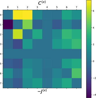
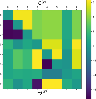
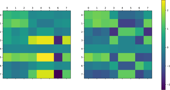
Figure 6.3: Comparison between matrices $C$ and $J$. Top left: the ${C^{({\sf x}{\sf x})}}$ box of matrix $C$ (upper right triangle) versus the ${J^{({\sf x}{\sf x})}}$ box of matrix $-J$. Top right: idem, but for ${C^{({\sf y}{\sf y})}}$ and ${J^{({\sf y}{\sf y})}}$. Bottom left: ${C^{({\sf x}{\sf y})}}$. Bottom right: ${J^{({\sf x}{\sf y})}}$. Mind that the $J$ matrix is such that negative matrix elements represent ferromagnetic couplings, or affine interactions. As a general trend, matrix $J$ is sparser than matrix $C$, as expected. The matrices $C$ and $J$ exhibit similar matrix elements, except in couples of coordinates involved in the same constraint. In the top row, the diagonal has been set to zero.

6.5 Longitudinal and Torsion interaction strengths

The ${n}\times{n}$ vertical, horizontal and oblique correlation matrices are defined as the corresponding correlations among landmark fluctuations: ${C^{({\sf x}{\sf x})}}_{ij}=\langle\Delta_{i,{\sf x}}\Delta_{j,{\sf y}}\rangle$, and the same for ${C^{({\sf x}{\sf y})}}$, ${C^{({\sf y}{\sf y})}}$. The whole $2{n}\times 2{n}$ correlation matrix $C$ is defined as $C_{\mu\nu}=\langle\Delta_{\mu}\Delta_{\nu}\rangle$, where the $2{n}$ Greek indices $\mu=i,{\sf c}_{i}$ denote the ${\sf c}_{i}={\sf x},{\sf y}$ coordinates of the $i$-th landmark. We define analogously the vertical, horizontal and oblique interaction matrices. The relation among these matrices is given by:

$$C=\left(\begin{array}[]{cc}{C^{({\sf x}{\sf x})}}&{C^{({\sf x}{\sf y})}}\\ {C^{({\sf x}{\sf y})}}^{\dagger}&{C^{({\sf y}{\sf y})}}\end{array}\right),\qquad J=\left(\begin{array}[]{cc}{J^{({\sf x}{\sf x})}}&{J^{({\sf x}{\sf y})}}\\ {J^{({\sf x}{\sf y})}}^{\dagger}&{J^{({\sf y}{\sf y})}}\end{array}\right),\qquad C=J^{-1}$$ (6.22)

where the $-1$ power means the pseudo-inverse operation.

In their turn, the longitudinal and torsion interaction matrices, $J^{\parallel}$, $J^{\perp}$, correspond to the displacements along, and normal to, the segment joining the landmarks $i$ and $j$, called $\hat{e}_{ij}=\langle\vec{r}_{ij}\rangle/r_{ij}$, where $\vec{r_{ij}}=\vec{r}_{j}-\vec{r}_{i}$ and $r_{ij}=|\langle\vec{r}_{ij}\rangle|$. These are defined so that the matrix elements $J_{ij}^{\parallel}$, $J_{ij}^{\perp}$ are the ${J^{({\sf x}{\sf x})}}_{ij}$ and ${J^{({\sf y}{\sf y})}}_{ij}$ couplings, but in a ($ij-$dependent) rotated basis such that the ${\sf x}$-axis coincides with the $i,j$ inter-landmark segment versor, ${\hat{e}}_{ij}$. Henceforth, the $J^{\parallel}$ and $J^{\perp}$ matrices are not obtained by a rotation of the original matrices ${J^{({\sf x}{\sf x})}}$ and ${J^{({\sf y}{\sf y})}}$. Instead, each $J^{\parallel}_{ij}$ element results from a whole inference procedure in a different basis depending on the couple $ij$. In particular, $J_{ij}^{\parallel}={J^{({\sf x}{\sf x})}}_{ij}(\hat{e}_{ij})$, where ${J^{({\sf x}{\sf x})}}(\hat{e}_{ij})$ is the inferred matrix obtained from the pseudo-inverse of matrix $C(\hat{e}_{ij})$ in a coordinate system in which the ${\sf x}$ axis coincides with the $ij$-segment (in other words, $C(\hat{e}_{ij})={\cal R}_{ij}^{{\dagger}}C{\cal R}_{ij}$, where ${\cal R}_{ij}$ is the 2D rotation matrix by the angle $-\alpha_{ij}$, and the matrix product is over the ${\sf x}$ and ${\sf y}$ blocks of matrix $C$).

We remark that there is less information in $J_{ij}^{\parallel}$, $J_{ij}^{\perp}$ (for all $i,j$) than in the whole effective interaction matrix $J$ (since the matrix whose matrix elements are ${J^{({\sf x}{\sf y})}}_{ij}(\hat{e}_{ij})$ is not $J^{\parallel}$, nor $J^{\perp}$).

We now provide a clearer interpretation of the longitudinal and torsion effective interaction matrices. $J_{ij}^{\parallel}$, $J_{ij}^{\perp}$ capture the relative relevance of the fluctuations around the average distance $\langle r_{ij}\rangle$, and of angle fluctuations around $\alpha_{ij}$, respectively. Large values of $J_{ij}^{\parallel}$ imply that the distance among $i$ and $j$ in the direction of its average axis is highly “locked”, i.e., it tends to exhibit small fluctuations, from sample to sample, around its most probable value. For instance (see figure 4 in the main text), a small fluctuation $\delta_{4,7}^{\parallel}=|(\vec{\Delta}_{4}-\vec{\Delta}_{7})\cdot\hat{e}_{4,7}|$ of the $4,7$-segment distance with respect to the average face ${\bm{\Delta}}={\bf 0}$ implies a large energy increment, $J^{\parallel}_{4,7}{\delta_{4,7}^{\parallel}}^{2}$ and, consequently, a large decrement of the probability density $\cal L$, proportional to $\exp(-J^{\parallel}_{4,7}{\delta_{4,7}^{\parallel}}^{2})$. Conversely, a fluctuation of the $6,7$ segment distance $\delta_{6,7}^{\parallel}$ will give rise to a small or non-significant decrement of the probability of the resulting facial vector since the longitudinal coupling constant $J^{\parallel}_{6,7}$ is small, a fact that highlights the prominent importance of the inter-landmark distance $r_{4,7}$ over $r_{6,7}$ in the process of facial discrimination. In the same way, fluctuations in the transversal components of both segments, $\delta_{4,7}^{\perp}$ and $\delta_{6,7}^{\perp}$ (and consequent fluctuations of the inter-landmark segment angles around $\alpha_{4,7}$ and $\alpha_{6,7}$), have a strong impact in their probability of being sculpted (i.e., in their perceived attractiveness), since both torsion coupling constants $J^{\perp}_{4,7}$ and $J^{\perp}_{6,7}$ are large in absolute value.

6.6 Dependence of $J$ on inter-landmark distances and angles

A different, interesting aspect of the matrix of effective interactions $J$ is the dependence of the interaction strengths among landmarks $i,j$ as a function of their average distance $\langle r_{ij}\rangle$ and average segment angle $\alpha_{ij}$. We stress that $\langle r_{ij}\rangle$ and $\alpha_{ij}$ are meta-parameters in the sense that that they are not codified in the database $\cal S$ and, hence, are not inferred (the facial vectors ${\bm{\Delta}}$ are actually fluctuations around the average single-landmark positions). From a cognitive point of view, one would expect that the interaction strengths $|{J^{({\sf x}{\sf x})}}_{ij}|$, $|{J^{({\sf y}{\sf y})}}_{ij}|$, $|{J^{({\sf x}{\sf y})}}_{ij}|$ among couples of nearby landmarks should tend to be stronger for smaller values of $r_{ij}$ or, at most, that they do not present an increasing trend (which would mean that farther away landmarks influence each other more than closer landmarks). In its turn, if the $ij$ coupling absolute value decreases with $\alpha_{ij}$, this would indicate the prominence of horizontal over vertical inter-landmark segments, and vice versa.

The data does not allow for sharp conclusions at these regards. However, and although the absolute value of the $J$ matrix elements do not show a clear trend with $r_{ij}$ nor with $\alpha_{ij}$, some interesting information can be retrieved from such analysis. Indeed, a moderate decreasing trend is observed in $|J^{\parallel}_{ij}|$ vs. $r_{ij}$, signifying that nearer landmarks tend to influence each other more than farther away landmarks, but only along the inter-$ij$ landmark segment, in the sense that only the longitudinal coupling presents such trend. Interestingly, the trend is lost when the ${\sf x}$, ${\sf y}$, ${\sf x}{\sf y}$ components of $J$ are plotted vs. $r_{ij}$. The absence of a clear trend with $\alpha_{ij}$ indicates lack of prominent importance of horizontal versus vertical inter-landmark segments.

We show in figures 6.4,6.5 the quantities $J^{\parallel}_{ij}$, $J^{\perp}_{ij}$ versus $\langle r_{ij}\rangle$ and $\alpha_{ij}$, respectively (see the main article). Although no clear trend is observed, it is apparent a moderate decreasing trend of $|J^{\parallel}_{ij}|$ versus $\langle r_{ij}\rangle$, as referred in the main article, and a slight decreasing trend of $|J^{\perp}_{ij}|$ versus $\alpha_{ij}$.

We notice that, in the notation of the article, negative values of $J$ indicate the tendency to positive correlations (a ferromagnetic interaction, in the statistical-physical language).

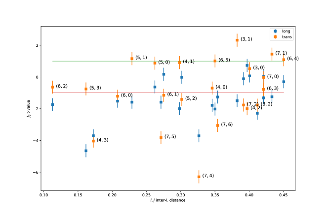
Figure 6.4: The t-value corresponding to the matrix elements $J^{\parallel}_{ij}$, $J^{\perp}_{ij}$ versus the inter-landmark average distance $\langle r_{ij}\rangle$.

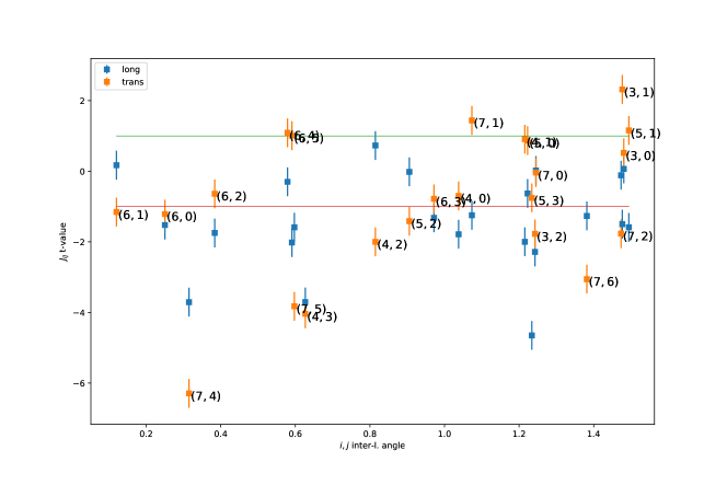
Figure 6.5: The t-value corresponding to the matrix elements $J^{\parallel}_{ij}$, $J^{\perp}_{ij}$ versus the angle subtended by $\hat{e}_{(ij)}$ with the ${\sf x}$-axis, $\alpha_{ij}$.

6.7 The Harmonic inference in the limit ${C^{({\sf x}{\sf x})}},{C^{({\sf y}{\sf y})}}\gg{C^{({\sf x}{\sf y})}}$

It can be shown that the solution of the inverse problem, at first order in the limit ${C^{({\sf x}{\sf y})}}\ll{C^{({\sf x}{\sf x})}},{C^{({\sf y}{\sf y})}}$), is:

$${J^{({\sf x}{\sf x})}} = {C^{({\sf x}{\sf x})}}^{-1}$$ (6.23a)

$${J^{({\sf y}{\sf y})}} = {C^{({\sf y}{\sf y})}}^{-1}$$ (6.23b)

$${J^{({\sf x}{\sf y})}} = -{J^{({\sf x}{\sf x})}}{C^{({\sf x}{\sf y})}}{J^{({\sf y}{\sf y})}}$$ (6.23c)

and that, in this limit, it is:

$$Z=\frac{(2\pi)^{n}}{(\det{J^{({\sf x}{\sf x})}}\,\det{J^{({\sf y}{\sf y})}}\,\det{J^{({\sf x}{\sf y})}})^{1/2}}$$ (6.24)

This can be shown by Gaussian integration, or approximating the inverse of the matrix

$$J=\left(\begin{array}[]{cc}{J^{({\sf x}{\sf x})}}&{J^{({\sf x}{\sf y})}}\\ {J^{({\sf x}{\sf y})}}^{\dagger}&{J^{({\sf y}{\sf y})}}\end{array}\right)$$ (6.25)

by using the first-order (in $A$) matrix expansion: $[B(1+A)]^{-1}\simeq(1-A)B^{-1}$, with $B=\left(\begin{array}[]{cc}{J^{({\sf x}{\sf x})}}&0\\ 0&{J^{({\sf y}{\sf y})}}\end{array}\right)$.

Indeed, the experimental matrices ${C^{({\sf x}{\sf x})}}$, ${C^{({\sf x}{\sf x})}}$ are larger than ${C^{({\sf x}{\sf y})}}$. The approximated solution, equation 6.23 is, consequently, a rather good approximation. In figure 6.6 we show this by comparing the exact ${J^{({\sf x}{\sf x})}}$, ${J^{({\sf y}{\sf y})}}$, ${J^{({\sf x}{\sf y})}}$ as different blocks of $J=C^{-1}$, versus the ones resulting from equation (6.23).

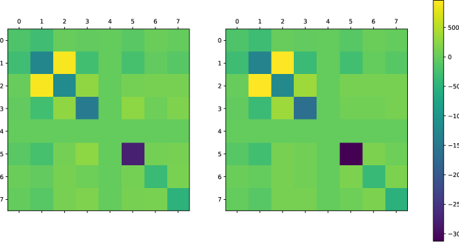
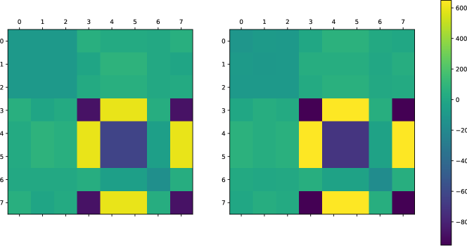
Figure 6.6: The comparison between the exact $J=C^{-1}$ and the approximated $J$ computed as in equation 6.23. Left column: approximated $J$. Right column: exact $J$. First, second and third row: ${J^{({\sf x}{\sf x})}}$, ${J^{({\sf y}{\sf y})}}$ and ${J^{({\sf x}{\sf y})}}$ respectively.

The relative influence of oblique correlations may be also assessed by defining a simpler model, that we will call the null-${\sf x}{\sf y}$ model, consisting in neglecting oblique interaction terms (taking ${J^{({\sf x}{\sf y})}}=0$). An even simpler model, that we will call dot model, consists in neglecting oblique interactions and supposing that the couplings ${J^{({\sf x}{\sf x})}}$ and ${J^{({\sf y}{\sf y})}}$ are equal:

$$H_{\rm dot}=\frac{1}{2}\sum_{i,j}J^{(\rm dot)}_{ij}\,{\vec{\Delta}}_{i}\cdot{\vec{\Delta}}_{j}$$ (6.26)

In this case the probability distribution is simply:

$${P}_{\rm dot}({\bf\Delta}_{\sf x},{\bf\Delta}_{\sf y}|J^{({\rm dot})})=\frac{(2\pi)^{n}}{\det J^{({\rm dot})}}\exp\left(-H_{({\rm dot})}[{\bf\Delta}_{\sf x},{\bf\Delta}_{\sf y}]\right)$$ (6.27)

where $J^{({\rm dot})}$ is the inverse matrix of $C^{({\rm dot})}_{ij}=\langle{\vec{\Delta}}_{i}\cdot{\vec{\Delta}}_{j}\rangle$.

We have assessed the efficiency of the dot and null-${\sf x}{\sf y}$ models by evaluating their efficiency in the classification task. As we show in section 6.16, neglecting the oblique correlations (in the null-${\sf x}{\sf y}$ model) and the anisotropy of vertical/horizontal correlations (in the dot model) leads to a poorer performance. This provides a quantitative assessment of the relative influence of these terms. We conclude that the influence of oblique correlations is crucial, and not negligible, in the facial perception process.

6.8 Two ways of inferring with constraints in the database of facial modifications

In section 6.2, we have exposed a method of MaxEnt inference (from pairwise interactions) from a database exhibiting linear constraints. Within this method, all the $D$ components of the vectors are considered, and inferred from, despite they are redundant. The resulting experimental correlation matrix $C$ is singular as it exhibits $D-r$ null eigenvalues, each one corresponding to a constraint. However, the influence of the constraints on the inferred model is subtracted by defining a probability distribution in the subspace of the coordinates that are invariant under the linear operation associated to the constraint. Mathematically, this is done through the pseudo-inverse operation (see eq. 6.14), which discards the subspace expanded by the eigenvectors corresponding with null eigenvalue. The corresponding inferred probability distribution corresponds to a system which is invariant under rescaling of the constraints $c_{j}$, equation (6.9).

An alternative method to infer $P$ avoiding the influence of constraints consists in inferring only a subset of $r$ non-redundant, unconstrained variables, in terms of which the correlation matrix has rank equal to $r$. As mentioned before and in the main article, this method may lead to a matrix of effective interactions leading to a less clear interpretation. The $J_{ij}$ elements will reflect in this case the influence of the constraints in the considered $r$ variables. Oppositely, with the null-mode subtraction method, the $J$ matrix represents a system which already satisfies the constraint (see section 6.4) and, for this reason, the $J_{ij}$ matrix elements do not reflect its influence on the data.

An illustration of these concepts is shown in the main article, where we compare matrices $C$ and $J$. The null-mode subtraction method provides a matrix $J$ which is actually sparser than matrix $C$. This does not occur when inferring from a reduced, non-redundant set of variables.

A further, particularly clear illustration is seen in terms of inter-landmark distances ${\bf d}=(d_{i})_{i=0}^{10}$, an alternative parametrization of the facial vectors $\bm{\Delta}$ (see the precise definition in [9] and in figure 6.2) in terms of 11 vertical or horizontal distances separating couples of landmarks. The function that maps a vector of inter-landmark distances $\bf d$ into a vector of landmark coordinates $\bm{\Delta}$ is one-to-one (and depends on some distances of the reference portrait). The distances $\bf d$ are subject to a constraint, reflecting the scale invariance of the problem [9]: $\sum_{i=1}^{4}d_{i}=1$, which signifies that all the distances $d_{i}$ are in units of the total face length (see figure 6.2). This constraint induces a null mode in the correlation matrix.

We now compare the effective interaction matrices corresponding to the two alternative ways of inference discussed before. We first calculate, see figure 6.7, the matrices $J^{(-k)}={C^{(-k)}}^{-1}$, the inverse of the $D-1\times D-1$ correlation matrices $C^{(-k)}_{ij}=\langle d_{i}d_{j}\rangle$ in which the $k$-th row and column have been removed, $i,j\neq k$. The matrices $J^{(-k)}$ are presented in figure 6.7 for $k=1,2,3,4$, compared with matrices ${C^{(-k)}}$.

We observe that the variables involved in the constraint result to be anticorrelated, $C^{(-k)}_{ij}<0$ when both $i,j$ are in the set $1,2,3,4$, a fact fact may be attributed to the presence of the constraint (e.g., vectors with larger distances $d_{1}$ tend to exhibit lower $d_{2}$’s, since, for all vectors, $d_{1}+d_{2}+d_{3}+d_{4}=1$). Indeed, also $-J^{(-k)}_{ij}<0$ for $1\leq i,j\leq 4$ and such that $i,j\neq k$ , $i\neq j$: it is necessary an anti-ferromagnetic interaction, or a statistical tendency of variable $i$ to decrease when variable $j$ increases, in order that the theoretical distribution associated to $J^{(k)}$ describes the statistics of the set of variables. Such statistical tendency is on the top of other statistical tendencies, of cognitive origin, not related to the constraint. In other words, the matrices $J^{(-k)}$ describe the data statistics of two different origins: those associated to the constraint, and those of cognitive origin.

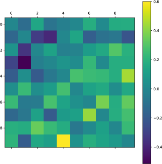
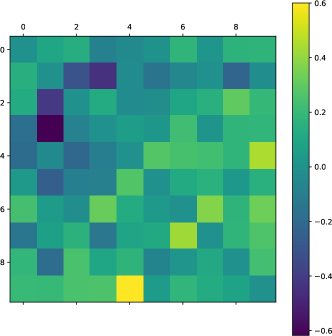
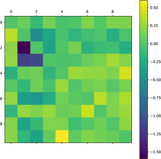
Figure 6.7: $\sf t$-value corresponding to the matrices $C^{(-k)}$ (upper right triangle) and $J^{(-k)}$ (bottom left triangle), in terms of inter-landmark distances, and avoiding the $k$-th distance, $d_{k}$. Top left, top right, bottom left and bottom right correspond, respectively, to $k=1,2,3,4$. We can observe that, for $i,j=1,2,3,4$, all the elements of $J_{ij}$ are positive. The diagonals of all matrices have been set to zero for a clearer comparison.

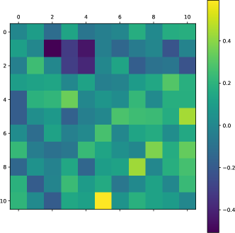
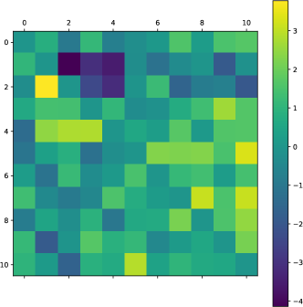
Figure 6.8: Matrices $C$ (upper right triangle) and $J$ (bottom left triangle) in terms of inter-landmark distances, using the whole, redundant set of distances and the null-mode subtraction method. Left: the matrix elements. Right: their $\sf t$-values. We see, at opposite with figure 6.7, that $J_{ij}<0$ for $i,j=1,2,3,4$. The diagonals have been set to zero for clearer comparison.

Second, in figure 6.8 we present the resulting effective interaction with the null-mode subtraction method, using as $J$ the pseudo-inverse of matrix $C$. We observe that, interestingly, all the couplings $-J_{ij}>0$ when both $i,j$ belong to the set $\{1,2,3,4\}$, implying a ferromagnetic effective interaction in the physical language, or a positive tendency of $d_{i}$ to increase when $d_{j}$ increases. In the pseudo-inverse case, $J$ represents the statistical effective interaction with the influence of the constraint subtracted. We learn information of cognitive, “physical” origin from $J$, that was veiled in the matrices $J^{(-k)}$’s, influenced by the presence of the constraint. In particular, we learn that the experimental subjects tend to prefer higher eyes, higher $d_{1}$, in facial modifications with larger noses, larger $d_{2}$.

In conclusion, the method of null-mode removal that we have used in this work allows, in general, for a more faithful interpretation of the effective parameters with respect to the alternative method of inferring from a set of non-redundant variables. It is important to stress that the generative model obtained from $J$ and from $J^{(-k)}$ is expected to be equally faithful. In other words, the difference discussed in this section regards but the interpretation of $J_{ij}$ elements, and only in situations in which the parameters actually admit an interpretation, as it is the case in the present and in other problems in biophysics and neurophysics. Indeed, the efficiency of both generative models as a classifier in the two groups of subjects (male/female, ${\cal S}={\cal S}_{A}\cup{\cal S}_{B}$), results to be equivalent, see section 6.16.

6.9 Average proportions and pairwise correlations

Facial beauty has been related to proportions since the Renaissance [41, 42], and most modern machine learning studies pose the problem in terms of proportions too [43, 44, 45, 6, 46, 47].

In the main text we have explained that the dataset is faithfully described by a MaxEnt probability distribution ${\cal L}({\bf x}|J,{\bf h})$, whose sufficient statistics is the matrix of pairwise correlations. We have also argued that, for a complete statistical description of the database of facial modifications, a model based on pairwise correlations is not enough. This implies that proportions, or ratios among facial distances, contains most of the information present in the database, although there is significant information, of cognitive origin, beyond proportions. We here justify such statement, making notice that the information regarding facial proportions is codified in the matrix of correlations among couples of facial distances.

Consider two facial coordinates, $r_{\alpha}$, $r_{\beta}$, referring to the ${\sf x}$ or ${\sf y}$ coordinates of two landmarks, say $i$ and $j$. We will consider their ratio, $r_{\alpha}/r_{\beta}$, which is the mathematical expression of a proportion. Calling $\bar{r}_{\alpha}=\langle r_{\alpha}\rangle$ the experimental average value, one has $r_{\alpha}=\bar{r}_{\alpha}+\Delta_{\alpha}$, by definition of displacement $\Delta_{\alpha}$. The displacements around the average, $\Delta_{\alpha}$, are much lower than the averages $\bar{r}_{\alpha}$, for all coordinate, $\alpha$ (see [9]). This justifies a Taylor expansion of $r_{\alpha}/r_{\beta}$ for low $\Delta$’s. Indeed, to the second order in the $\Delta$’s:

$$\frac{r_{\alpha}}{r_{\beta}}=\frac{\bar{r}_{\alpha}}{\bar{r}_{\beta}}\left(1-\frac{\Delta_{\beta}}{\bar{r}_{\beta}}\right)+\frac{\Delta_{\alpha}}{\bar{r}_{\beta}}-\frac{\Delta_{\alpha}\Delta_{\beta}}{\bar{r}_{\beta}}+O\left[\left(\frac{\Delta}{r}\right)^{2}\right]$$ (6.28)

The experimental average of this expression $\langle r_{\alpha}/r_{\beta}\rangle$ is, up to an additive constant, equal to $-(1/\bar{r}_{\beta}^{2})\langle\Delta_{\alpha}\Delta_{\beta}\rangle$ (having used that $\langle\Delta_{\alpha}\rangle=0$). Hence, the average proportions are completely determined, in the case of small displacements, by the pairwise correlations.

6.10 Harmonic interactions and elastic constants

In the main article we have explained that the 2-MaxEnt model for vectors of facial distance displacements $\bm{\Delta}$ may be interpreted as the Maxwell-Boltzmann distribution corresponding to a set of particles in 2D interacting through a set of three anisotropic, couple-dependent springs, in the canonical ensemble. We will here justify such statement. We will focus in a couple of landmarks, say $i,j$. We will call $x_{i}$, $x_{j}$ the components of the position of landmarks $i,j$ over two versors in the plane, $\hat{e}^{(i)}$, $\hat{e}^{(j)}$, respectively. In other words: $x_{i}=\vec{r}_{i}\cdot{\hat{e}^{(i)}}$ and the same for $j$, in the notation of the main article. Given the coordinates $x_{i}$, $x_{j}$, and if $\hat{e}^{(i)}=\hat{e}^{(j)}$, the quantity $\delta_{ij}=x_{i}-x_{j}-(\bar{x}_{i}-\bar{x}_{j})$ is the change in the distance among $i$ and $j$ with respect to the average vector, and along the common axis $\hat{e}^{(i)}$. For example, if the versor is the vertical axis, $\delta_{ij}$ indicates the shift of the vertical distance among landmarks $i,j$ with respect to the average distance among $i,j$. We will define the elastic interaction energy as $(1/2)k_{ij}\delta_{ij}^{2}$, which is minimum and equal to zero whenever the distance among $i,j$ is unchanged with respect to the average, $\delta_{ij}=0$, regardless on the single-landmark displacements $x_{i}$, $x_{j}$. We make notice that expanding, again, in $\delta_{i}=x_{i}-\bar{x}_{i}$ to the second order in $\delta_{i}$ and $\delta_{j}$, it is: $\delta_{ij}^{2}=-2\delta_{i}\delta_{j}+b+O[\delta^{2}]$, where $b$ is a constant in $\delta_{i}$ and $\delta_{j}$, depending only on $\bar{x}_{i}$ and $\bar{x}_{j}$. Henceforth, the elastic interaction energy, ${\cal E}=(1/2)k_{ij}\delta_{ij}^{2}$ is, up to a constant, and for small fluctuations around the average, $=-2\delta_{i}\delta_{j}k_{ij}$, which is the form of the interaction energy in the pairwise Hamiltonian model with the following relation among elastic constant and effective interaction matrix element: $k_{ij}=-(1/2)J_{ij}$. Fixing, for example, $\hat{e}^{(i)}=\hat{e}^{(j)}=\hat{e}_{ij}$, the versor joining the average position of both landmarks, $\hat{e}_{ij}=\langle\vec{r}_{i}-\vec{r}_{j}\rangle/|\langle\vec{r}_{i}-\vec{r}_{j}\rangle|$, we have that $k_{ij}^{\parallel}=-(1/2)J^{\parallel}_{ij}$, and idem for the perpendicular components of $\vec{r}$, $\perp$, and for the vertical, horizontal and oblique components of $\vec{r}$.

6.11 Cognitive origin of non-linear correlations

In the experiments presented in [9], the subject sculpts her/his ideal facial modification through the interaction with a software called FACEXPLORE, based on genetic and image deformation algorithms. The sculpture process consists in a sequence of multiple left/right choices among couples of facial images, eventually leading to an estimation of the ideal modification according to the subject. Actually, the genetic algorithm performs the recombination and mutation steps, while the single experimental subject actually plays the role of the selection step, through her/his choices.

The genetic algorithm used (called Differential Evolution) processes different coordinates independently (see the SI of [9]). The only correlation among coordinates is expected to be induced by the selection process, performed by the human subject. As a consequence, one should expect that the only origin of correlations among coordinates in the populations sculpted by subjects (by the same or by different subjects) are of cognitive nature.

In fact, this is not the case: part of the correlations that one observes experimentally are due to an artifact of the algorithm. In a null-model experiment with a random sequence of left/right choices, the resulting database exhibits significant non-linear correlations of order $2$ and $3$ among facial coordinates. The correlations of order three, $\langle\Delta_{i}\Delta_{j}\Delta_{k}\rangle$, are statistically compatible with the 3-order correlations observed in the human experiment [9].

The solution of this paradox is that, while the genetic algorithm does not introduces correlations in the recombination and mutation steps, it actually may amplify the correlations among facial coordinates which are present in the initial condition of the null-model genetic population of facial vectors. Such initial populations are trivially correlated, since some constraints were imposed in the definition of the face space: mainly $\sum_{i=1}^{4}d_{i}=1$ and $d_{10}<d_{5}$ (see section 6.8 and figure 6.2).

In reference [9] we proposed a method to “subtract” the influence of the a priori, non-cognitive or artifact correlations present in the null model experiment, from the cognitive true correlations that we observed. The method revealed that the artifact pairwise correlations did not have a significant impact in the results. We suspect that correlations of higher order may be, instead, significantly influenced by the artifact effect.

In the main article text, we have explained that non-linear inference algorithms allow for a much better classification of the database according to the gender of the experimental subject. This fact implies that, quite interestingly, the differences between facial vectors sculpted by males and by females is encoded in non-Gaussian correlations, beyond proportions ($p=2$), beyond triplets and perhaps quadruplets of facial distances. In the main article, we have also explained that this may imply that such differences codified in non-Gaussian correlations are of cognitive order, i.e., that male and female subjects’ do prefer facial variations differing in non-Gaussian correlations and, in particular, that humans evaluate quantities that are much more complicated than proportions, when forming an impression about a face. The fact that the introduction of non-linearity helps in a gender classification task, which reflects real and well-known cognitive differences, may suggest so.

An alternative explanation is that the distinguishable differences among male and female preferred facial variations are all codified in pairwise effective interactions only (say, roughly speaking, that males and females differ only in the $J$ matrix, if it could be measured without bias). The non-linear interactions would turn anyway relevant for the classification, since the correlations propagated by the genetic algorithm are coupled to the ones induced by the subject: subjects differing only in $J$ would also induce, by means of the artifact, differences in the correlations of higher order.

Further experiments are needed to clarify this issue.

6.12 Generality of the MaxEnt models

Crucially, the two models of unsupervised inference presented in the main text exhibit a wide generality, going beyond the particular database that we infer in this work. (1) First, the inferred set of facial vectors may be composed by facial images selected according to any criterion: selected by a pool of subjects among real facial images or by a single individual (in this case the distribution ${\cal L}(\cdot|\bm{\theta})$ would probabilistically characterise the single subject’s preferred region in face-space); selected according to a criterion different from attractiveness; even not having been selected by subjects but chosen according to some objective criterion as age or gender (${\cal L}({\bf f}|\bm{\theta})$ would hence represent the probability that a facial image characterised by the facial vector ${\bf f}$ presents the desired feature). (2) Second, they can be used to infer any other database of images characterised by the geometric positions of facial (or, in general body) landmarks. (3) Third, these models may be immediately extended to process also non-geometric degrees of freedom (treating the texture and geometric degrees of freedom on the same footing [36]).

6.13 Learning in the non-linear MaxEnt model.

The 3-MaxEnt model parameters are $n_{\rm p}=D+D(D+1)/2+D(D-1)(D-2)/6$ independent components of the interaction tensors $\bm{\theta}=({\bf h},J,Q)$ of order 1,2,3. Their value in the article is fixed by Maximum Likelihood, i.e., by the maximisation of the joint database likelihood, as in equation (6.3). In the case of the 3-MaxEnt model, we have estimated numerically the maximum likelihood value of the parameters $\bm{\theta}^{*}$ by means of a numerical maximisation of the joint database likelihood by deterministic gradient ascent, using an algorithm that will be presented in a dedicated publication.

A discrete sequence of interaction tensors $\bm{\theta}(t)$ are recursively updated according to a deterministic gradient ascent rule: $\bm{\theta}(t+1)=\bm{\theta}(t)+\eta_{\bm{\theta}}\,\partial_{\bm{\theta}}\left[\ln{\cal L}({\cal S}|\bm{\theta})\right]_{\bm{\theta}(t)}$, using a learning rate $\eta_{\bm{\theta}}$ depending on the tensor that is being update. We use $\eta_{J}=10^{-2}$ for the matrices and $\eta_{Q}=10^{-3}$ for the 3-order tensors. The rule is iterated until a quasi-stationary state of the associated test-set joint likelihood is achieved within its statistical error. In particular, the stopping criterion is that the joint test database likelihood increment is lower than $1\%$ in an interval of 10 epochs (an epoch is an iteration of all the tensor elements). As initial condition of the learning dynamics, we choose ${\bf h}={\bf 0}$, $J=\mathbb{I}_{D}$, $Q=0$.

At a given epoch, $t$, of the gradient ascent iteration, the gradient of the joint likelihood with respect to the effective interaction components involves a theoretical correlator (of order 1,2 or 3) according to the current value of the couplings. For instance: $\left[\partial_{J_{\alpha\beta}}\ln{\cal L}({\cal S}|\bm{\theta})\right]_{\bm{\theta}(t)}=\langle\Delta_{\alpha}\Delta_{\beta}\rangle_{{\cal L}({\cdot}|\bm{\theta}(t))}-\langle\Delta_{\alpha}\Delta_{\beta}\rangle$. Such theoretical correlator is in its turn estimated by means of a Markov Chain Monte Carlo (MCMC) Metropolis algorithm for the sampling of configurations from the theoretical distribution at the corresponding epoch, ${\cal L}(\cdot,\bm{\theta}(t))$. For such MCMC algorithm, we use a number of sweeps $=10^{6}$ in each epoch. The MCMC vectors ${\bm{\Delta}}$ are initialised as normal variables with variance equal to their empirical variance, and the Metropolis trials are chosen uniformly in the interval $\Delta_{\alpha}\in[-5\sigma_{\alpha},5\sigma_{\alpha}]$, where $\sigma_{\alpha}$ is the empirical standard deviation of $\Delta_{\alpha}$. Finally, the evaluation of the joint database likelihood in every step of the gradient ascent maximisation algorithm requires the evaluation of the partition function $Z_{3}$. This is performed by means of a Mayer expansion of the energy around the Gaussian model, to the first order in $J^{(3)}/J^{(2)}$.

6.14 Learning the database with the Gaussian Restricted Boltzmann Machine

Definition of the model. The Gaussian Restricted Boltzmann Machine (GRBM) is a type of generative stochastic two-layered Artificial Neural Network [48, 49, 50, 51]. It is a generalisation of the Restricted Boltzmann Machine (RBM) model [52], that learns a probabilistic generative model for real-valued vectors: the visible neurons in the input layer, $\bm{v}$, assume real values. The value of the hidden neurons $\bm{h}$ is, instead, binary, $h_{j}=0,1$. The state of the $N_{\rm v}$ visible $\bm{v}=(v_{i})_{i=1}^{N_{\rm v}}$ and $N_{\rm h}$ hidden $\bm{h}=(h_{i})_{i=1}^{N_{\rm h}}$ neurons is described by an energy-based probability density:

$$p(\bm{v},\bm{h}|\bm{\theta})=\frac{1}{Z_{\bm{\theta}}}e^{-E(\bm{v},\bm{h}|\bm{\theta})}$$ (6.29)

in terms of the parameters $\bm{\theta}=\{W,\bm{b},\bm{c},\bm{\sigma}\}$, to be inferred in the learning process. $W$ is a real ${N_{\rm v}\times N_{\rm h}}$ matrix coupling real and visible variables, while $\bm{c}$, $\bm{\sigma}$ are $N_{\rm v}$-dimensional real vectors representing the bias over the visible neurons and their standard deviation, respectively, while $\bm{b}$ is a real $N_{\rm h}$-dimensional vector representing the bias over hidden neurons. ${Z_{\bm{\theta}}}$ is a normalising constant, depending on the parameters. The function energy $E$ is defined so that the conditional probability distribution $p(\bm{v}|\bm{h},\bm{\theta})$ results to be a normal, independent distribution over visible variables. It assumes the form:

$$E(\bm{v},\bm{h})=-\sum_{i=1}^{N_{\rm v}}\sum_{a=1}^{N_{\rm h}}\frac{W_{ia}v_{i}h_{a}}{\sigma_{i}^{2}}+\sum_{i=1}^{N_{\rm v}}\frac{\big{(}v_{i}-c_{i}\big{)}^{2}}{2\sigma_{i}^{2}}-\sum_{a=1}^{N_{\rm h}}h_{a}b_{a}$$ (6.30)

The GRBM probabilistic generative model is obtained through a marginalisation of the hidden variables: $p(\bm{v}|\bm{\theta})=\sum_{\bm{h}}p(\bm{v},\bm{h}|\bm{\theta})$. This model (as far as the hidden neurons are binary) is known to induce non-linear interactions among the visible variables, up to order $p=N_{\rm v}$ in the most general case [53].

Learning protocol. We have trained the model over a set of redundant or non-redundant data, obtaining equivalent results. As a learning algorithm we have used gradient ascent through persistent contrastive divergence with ${\sf k}=1$ Monte Carlo step, along with mini-batch learning with batch size $B$ [49], and an epoch-depending variable learning rate, $\eta$, increasing linearly with the number of epochs. We have set the value of the learning hyperparameters to: number of steps $n_{s}=2\cdot 10^{5}$, batch size $B=200$, momentum $\mu=0$, initial learning rate $\eta_{0}=2\cdot 10^{-3}$. The learning rate slope is set such that $\eta_{n_{s}}=2\cdot 10^{-5}$. The parameters $W$, $\bm{b}$ and $\bm{c}$ are initialized following a standard procedure [54, 55]:

$$W_{ia}=\chi_{ia}\sqrt{\frac{6}{N_{V}+N_{\rm h}}}\ ,\quad\chi_{ia}\in(-1,1)\quad\forall i,a$$ (6.31a)

$$b_{a}=-\frac{1}{2}(||\bm{W}_{*,a}+\bm{c}||+||\bm{c}||)+\log(0.1)\quad\forall a$$ (6.31b)

$$c_{i}=0\quad\forall i$$ (6.31c)

$$\sigma_{i}=1/2\quad\forall i$$ (6.31d)

As equilibration test we have verified that the test-set joint likelihood is stationary as a function of the number of epochs, within its associated standard deviation. We have performed an assessment of the algorithm efficiency as a function of the number of hidden neurons, $N_{\rm h}$. As shown in figure 6.9, both the test and training-set joint likelihood exhibit a monotonous increasing behaviour vs $N_{\rm h}$, showing no sign of severe overfitting. The auROC score saturates at its maximum value for values $N_{\rm h}\gtrsim 8N_{\rm v}$, with $N_{\rm v}=10$, confirming this picture. We have consequently considered, for the analysis performed in the main article, $N_{\rm h}=100$.

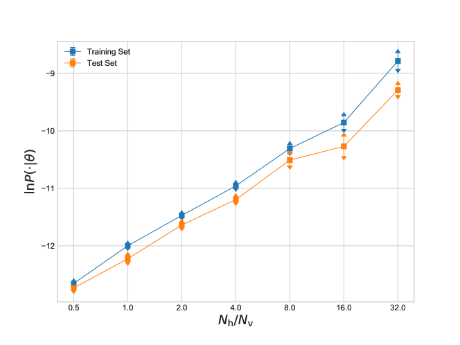
Figure 6.9: Training and test-set log-likelihood as a function of the ratio $N_{\rm h}/N_{\rm v}$, each point has been obtained averaging over 5 realizations of the learning, once the stationary state of the train log-likelihood has been achieved.

Before GRBM learning, the data has been pre-processed eliminating $6$ redundant coordinates, subtracting the average (of the whole database, not of the $\{A,B\}\times\{{\rm train},{\rm test}\}$ datasets separately) and standardising, or dividing each vector component-wise by the vector of standard deviations along the whole set. We have learned the dataset with a variable number of hidden neurons $N_{\rm h}$, from $N_{\rm h}=D$ to $N_{\rm h}=16\,D$.

Afterwards, for the sake of the classification, the model has been trained over the $A,B$ training databases separately, leading to two sets of parameters $\bm{\theta}_{A}$, $\bm{\theta}_{B}$ and, consequently, to a likelihood function ${\cal L}_{\rm RBM}(\cdot|\bm{\theta}_{A,B})$. Afterwords, the score ${\sf s}(\tilde{\bf r})=\ln{\cal L}(\tilde{\bf r}|\bm{\theta}_{A})-\ln{\cal L}(\tilde{\bf r}|\bm{\theta}_{B})$ is defined for every standardised and non-redundant vector $\tilde{\bf r}$ of the $A,B$ test-sets. Such score is used to construct the ROC curve and scores shown in the main article.

6.15 Classification with the Random Forest algorithm

In the random forest classification presented in the main article and in figure 6.10, we have used the Random Forest Classifier [56, 57], using $1000$ trees created from bootstrapped sub-sample and with nodes expanded until all leaves are pure. As an assessment of the single-split quality we have considered the Gini function. The number of random features considered in the best split choice is equal to ${\sf int}({\sf sqrt}(D))$, where $D=16$ is the number of features.

6.16 Detailed comparison among several classification methods

We now present a more detailed analysis of all the classification algorithms that we have considered for the classification of the database according to the subjects’ gender. In table 6.1 we present a systematic comparison of the auROC value [35], a standard estimator of the classification accuracy (the area under the corresponding ROC curves in figure 6.10), associated to the classification according the various algorithms. In particular, 2-MaxEnt approximated is the 2-Maxent model resulting from the approximation in equation (6.23); 2-MaxEnt null-${{\sf x}{\sf y}}$ is the model consisting neglecting the oblique interactions, ${J^{({\sf x}{\sf y})}}=0$; 2-MaxEnt dot is defined in equation (6.27); 1-MaxEnt dot is defined by inferring the external fields only (and taking the interaction matrix $J$, required for the normalisation of $P$, as a diagonal matrix whose diagonal is equal to the inverse variance of each variable).

The results of table 6.1 and of figure 6.10 confirm the picture presented in the main article. The value of the single facial distances (in units of the facial length) are not enough for an accurate description of the database of facial modifications. The introduction of pairwise effective interactions, which explain proportions, or ratios of facial coordinates, induces a notable improvement in the statistical description. Moreover, oblique effective interactions (coupling the ${\sf x}$ coordinate of one landmark with the ${\sf y}$ coordinate of another landmark) result a fundamental ingredient. Finally, a crucial role, at least for the sake of the classification according to the subjects’ gender, is plaid by effective interactions of higher order: $p=3$ (3-MaxEnt) and $p>3$ (GRBM and random forest). We conclude that the classification is a valid method for the assessment of the assessment of the relative relevance of the various terms.

Remarkably, an as we anticipated in section 6.8, the algorithm used to avoid the constraints (inferring from a reduced, non-redundant set of variables, or using the null-mode subtraction method) do not change the efficiency of the classification. Indeed, the model that we call 2-MaxEnt non-redundant in table 6.1 and in figure 6.10 is identical to 2-MaxEnt but in terms of a subset of $10$ non-redundant variables. Its auROC estimator and ROC curve are statistically distinguishable from 2-MaxEnt (with $16$ variables and null-mode subtraction).

Table 6.1:

algorithm	auROC
random forest	0.995
GRBM	0.988
3-MaxEnt	0.930
2-MaxEnt	0.848
2-MaxEnt non-redundant	0.846
2-MaxEnt approximated	0.830
2-MaxEnt null-${{\sf x}{\sf y}}$	0.770
2-MaxEnt dot	0.745
1-MaxEnt	0.654

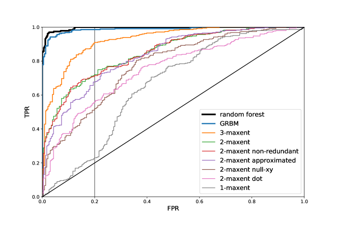
Figure 6.10: ROC curves of all the models defined in the text. The order of the model in the legend (and in table 6.1) is also the order with which the corresponding curve crosses the vertical line at FPR=0.2.

6.17 Inter- and intra-subject correlations and errors.

The set of facial vectors sculpted by a single subject, $\{{\bf r}^{(v,i)}\}_{i=1}^{\cal N}$, are not the result of independent sculpting experiments. They are, rather, correlated as far as they are the outcome genetic population of facial vectors that evolved according to a stochastic evolutionary algorithm coupled to a sequence of choices performed by the experimental subject [9]. Consequently, it is crucial to subtract the effect of intra-subject (or intra-genetic population) correlations among facial vector components from the inter-subject correlations. On the one hand, one may define the bare correlation matrix, accounting from both sources of correlations, defined by summing over both subject and population indices: $C_{\alpha\beta}=\langle\Delta_{\alpha}\Delta_{\beta}\rangle$. On the other hand, the inter-subject correlation matrix accounts only for the inter-subject correlation, and is defined as $\bar{C}_{\alpha\beta}=\overline{(1/{n_{\rm s}})\sum_{v^{\prime}=1}^{{n_{\rm s}}}\Delta_{\alpha}^{v(v^{\prime}),i(v^{\prime})}\Delta_{\beta}^{v(v^{\prime}),i(v^{\prime})}}$, where $v(v^{\prime})$ and $i(v^{\prime})$ are random indices in the sets $1,\ldots,{n_{\rm s}}$ and $1,\dots,{\cal N}$ respectively, uncorrelated among them and on $v^{\prime}$, and the overline $\overline{\cdot}$ means an average over a sufficiently high number of realisations of the set of indices $v(v^{\prime})$, $i(v^{\prime})$ for $v^{\prime}=1,\ldots,{n_{\rm s}}$. The statistical uncertainty associated to the inter-subject correlation, $\sigma_{C_{\alpha\beta}}$, is the standard deviation of the overline argument under many realisations of the set of indices (in other words, a Bootstrap error using only one vector for subject in each Bootstrap sampling, see the SI of ref. [9]). Consequently, the error associated to the inter-subject correlation is of order $\sim{n_{\rm s}}^{-1/2}$, and not of order $\sim S^{-1/2}$ as that of the bare correlation matrix. Analogously, we also define inter-subject and bare $3$-component correlations.

If the inferred model should describe the probability of a given facial vector to have been selected by any subject in the database, then it should be committed to reproduce by construction the inter-subject (not the bare) correlations. Otherwise, the probabilistic generative models may also simply describe the whole set of facial vectors in the [9] experiments, hence accounting also for the intra-subject correlations; the corresponding MaxEnt models would reproduce by construction the $2$ or $3$ bare correlations in this case. In our data analysis software one can specify whether the $2,3$ MaxEnt inferred model reproduce bare or inter-subject correlations. In this article, some results (the reproduction of angle histograms and the analysis of $J$ matrices) correspond to the inter-subject inference models. The classification tests have, instead, been done with the bare models. For the sake of classification, we have simply tested the ability of the algorithm to capture any useful correlation, regardless of its origin, cognitive or algorithmic. The bare inference models suffer less from the curse of dimensionality since the effective database size is $S={\cal N}{n_{\rm s}}$ instead of ${n_{\rm s}}$.

7 Bibliography

References

- [1] Mirella Walker and Thomas Vetter “Changing the personality of a face: Perceived Big Two and Big Five personality factors modeled in real photographs.” In Journal of personality and social psychology 110.4, 2016, pp. 609
- [2] Anthony Little, Benedict Jones and Lisa DeBruine “Facial attractiveness: evolutionary based research” In Philosophical Transactions, 2011 DOI: http://dx.doi.org/10.1098/rstb.2010.0404
- [3] David A. Leopold and Gillian Rhodes “A Comparative View of Face Perception” In Journal of comparative psychology (Washington, D.C. : 1983) 124.3, 2010, pp. 233–251 DOI: 10.1037/a0019460
- [4] D. Bzdok et al. “ALE meta-analysis on facial judgments of trustworthiness and attractiveness” In Brain Structure and Function 215.3-4, 2011, pp. 209–223 DOI: 10.1007/s00429-010-0287-4
- [5] Amanda C. Hahn and David I. Perrett “Neural and behavioral responses to attractiveness in adult and infant faces”, 2014
- [6] A. Laurentini and A. Bottino “Computer analysis of face beauty: A survey” In Computer Vision and Image Understanding 125, 2014, pp. 184–199 DOI: 10.1016/j.cviu.2014.04.006
- [7] Anthony C. Little “Facial attractiveness” In Wiley Interdisciplinary Reviews: Cognitive Science 5.6 John Wiley & Sons, Inc., 2014, pp. 621–634 DOI: 10.1002/wcs.1316
- [8] Randy Thornhill and Steven W. Gangestad “Facial attractiveness” In Trends in Cognitive Sciences 3.12, 1999, pp. 452–460 DOI: http://dx.doi.org/10.1016/S1364-6613(99)01403-5
- [9] M. Ibáñez-Berganza, A. Amico and V. Loreto “Subjectivity and complexity of facial attractiveness” In Scientific Reports 9 Nature Publishing Group, 2019, pp. 8364 URL: https://www.nature.com/articles/s41598-019-44655-9
- [10] Tim Valentine, Michael B. Lewis and Peter J. Hills “Face-space: A unifying concept in face recognition research” In The Quarterly Journal of Experimental Psychology 69.10 Routledge, 2016, pp. 1996–2019 DOI: 10.1080/17470218.2014.990392
- [11] Michael Cunningham et al. “Their Ideas of Beauty Are, On the Whole, the Same as Ours” In Journal of Personality and Social Psychology 68, 1995 DOI: http//doi.org/10.1037/0022-3514.68.2.261
- [12] R.. Edler “Background Considerations to Facial Aesthetics” In Journal of Orthodontics 28.2, 2001, pp. 159–168 DOI: 10.1093/ortho/28.2.159
- [13] Luigi Maria Galantucci, Eliana Di Gioia, Fulvio Lavecchia and Gianluca Percoco “Is principal component analysis an effective tool to predict face attractiveness? A contribution based on real 3D faces of highly selected attractive women, scanned with stereophotogrammetry” In Medical & Biological Engineering & Computing 52.5, 2014, pp. 475–489 DOI: 10.1007/s11517-014-1148-8
- [14] Nikolaas N. Oosterhof and Alexander Todorov “The functional basis of face evaluation” In Proceedings of the National Academy of Sciences 105.32, 2008, pp. 11087–11092 DOI: 10.1073/pnas.0805664105
- [15] A. Todorov and N.. Oosterhof “Modeling Social Perception of Faces [Social Sciences]” In IEEE Signal Processing Magazine 28.2, 2011, pp. 117–122 DOI: 10.1109/MSP.2010.940006
- [16] Yaniv Abir et al. “The determinants of consciousness of human faces” In Nature Human Behaviour, 2017, pp. 1 DOI: 10.1038/s41562-017-0266-3
- [17] E.. Jaynes “Information Theory and Statistical Mechanics” In Phys. Rev. 106 American Physical Society, 1957, pp. 620–630 DOI: 10.1103/PhysRev.106.620
- [18] Johannes Berg “Statistical mechanics of the inverse Ising problem and the optimal objective function” In Journal of Statistical Mechanics: Theory and Experiment 2017.8, 2017, pp. 083402 URL: http://stacks.iop.org/1742-5468/2017/i=8/a=083402
- [19] H. Nguyen, Riccardo Zecchina and Johannes Berg “Inverse statistical problems: from the inverse Ising problem to data science” In Advances in Physics 66.3 Taylor & Francis, 2017, pp. 197–261 DOI: 10.1080/00018732.2017.1341604
- [20] Andrea De Martino and Daniele De Martino “An introduction to the maximum entropy approach and its application to inference problems in biology” In Heliyon 4.4, 2018, pp. e00596 DOI: https://doi.org/10.1016/j.heliyon.2018.e00596
- [21] Timothy R Lezon et al. “Using the principle of entropy maximization to infer genetic interaction networks from gene expression patterns” In Proceedings of the National Academy of Sciences 103.50 National Acad Sciences, 2006, pp. 19033–19038
- [22] Elad Schneidman, Michael J Berry II, Ronen Segev and William Bialek “Weak pairwise correlations imply strongly correlated network states in a neural population” In Nature 440.7087 Nature Publishing Group, 2006, pp. 1007
- [23] Jonathon Shlens et al. “The structure of multi-neuron firing patterns in primate retina” In Journal of Neuroscience 26.32 Soc Neuroscience, 2006, pp. 8254–8266
- [24] William Bialek and Rama Ranganathan “Rediscovering the power of pairwise interactions” In arXiv preprint arXiv:0712.4397, 2007
- [25] Aonan Tang et al. “A maximum entropy model applied to spatial and temporal correlations from cortical networks in vitro” In Journal of Neuroscience 28.2 Soc Neuroscience, 2008, pp. 505–518
- [26] Martin Weigt et al. “Identification of direct residue contacts in protein–protein interaction by message passing” In Proceedings of the National Academy of Sciences 106.1 National Acad Sciences, 2009, pp. 67–72
- [27] Yasser Roudi, Erik Aurell and John A Hertz “Statistical physics of pairwise probability models” In Frontiers in computational neuroscience 3, 2009, pp. 22 DOI: 10.3389/neuro.10.022.2009
- [28] Gasper Tkacik et al. “Spin glass models for a network of real neurons” In arXiv preprint arXiv:0912.5409, 2009
- [29] Greg J Stephens and William Bialek “Statistical mechanics of letters in words” In Physical Review E 81.6 APS, 2010, pp. 066119
- [30] Thierry Mora, Aleksandra M Walczak, William Bialek and Curtis G Callan “Maximum entropy models for antibody diversity” In Proceedings of the National Academy of Sciences 107.12 National Acad Sciences, 2010, pp. 5405–5410
- [31] Faruck Morcos et al. “Direct-coupling analysis of residue coevolution captures native contacts across many protein families” In Proceedings of the National Academy of Sciences 108.49, 2011, pp. E1293–E1301 DOI: 10.1073/pnas.1111471108
- [32] William Bialek et al. “Statistical mechanics for natural flocks of birds” In Proceedings of the National Academy of Sciences 109.13, 2012, pp. 4786–4791 DOI: 10.1073/pnas.1118633109
- [33] Nan Wang, Jan Melchior and Laurenz Wiskott “An Analysis of Gaussian-Binary Restricted Boltzmann Machines for Natural Images” In Proc. 20th European Symposium on Artificial Neural Networks, Computational Intelligence and Machine Learning, Apr 25–27, Bruges, Belgium, 2012, pp. 287–292
- [34] Nan Wang, Jan Melchior and Laurenz Wiskott “Gaussian-binary Restricted Boltzmann Machines on Modeling Natural Image Statistics” In CoRR abs/1401.5900, 2014 arXiv: http://arxiv.org/abs/1401.5900
- [35] Kevin Murphy “Machine Learning: A Probabilistic Perspective” The MIT Press, 2012
- [36] Le Chang and Doris Y. Tsao “The Code for Facial Identity in the Primate Brain” In Cell 169.6, 2017, pp. 1013–1028.e14 DOI: 10.1016/j.cell.2017.05.011
- [37] Anthony C. Little, D. Burt and David I. Perrett “What is good is beautiful: Face preference reflects desired personality” In Personality and Individual Differences 41.6, 2006, pp. 1107–1118 DOI: https://doi.org/10.1016/j.paid.2006.04.015
- [38] Jan Melchior “PyDeep” GitHub, https://github.com/MelJan/PyDeep.git, 2017
- [39] Andrea Cavagna et al. “Short-range interactions versus long-range correlations in bird flocks” In Phys. Rev. E 92 American Physical Society, 2015, pp. 012705 DOI: 10.1103/PhysRevE.92.012705
- [40] Leo P Kadanoff “Statistical physics: statics, dynamics and renormalization” World Scientific Publishing Company, 2000
- [41] Judith H Langlois et al. “Maxims or myths of beauty? A meta-analytic and theoretical review.” In Psychological bulletin 126.3 American Psychological Association, 2000, pp. 390
- [42] Farhad B. Naini, James P. Moss and Daljit S. Gill “The enigma of facial beauty: Esthetics, proportions, deformity, and controversy” In American Journal of Orthodontics and Dentofacial Orthopedics 130.3, 2006, pp. 277–282 DOI: 10.1016/j.ajodo.2005.09.027
- [43] Hatice Gunes and Massimo Piccardi “Assessing facial beauty through proportion analysis by image processing and supervised learning” In Science Direct, 2006 DOI: http://dx.doi.org/10.1016/j.ijhcs.2006.07.004
- [44] Jintu Fan et al. “Prediction of facial attractiveness from facial proportions” Brain Decoding In Pattern Recognition 45.6, 2012, pp. 2326–2334 DOI: http://dx.doi.org/10.1016/j.patcog.2011.11.024
- [45] F. Chen and D. Zhang “Evaluation of the Putative Ratio Rules for Facial Beauty Indexing” In 2014 International Conference on Medical Biometrics, 2014, pp. 181–188 DOI: 10.1109/ICMB.2014.38
- [46] Hui Shen, Desmond K.P. Chau and Jianpo et all. Su “Brain responses to facial attractiveness induced by facial proportions: evidence from an fMRI study” In Nature, 2016 DOI: http://doi.org/doi:10.1038/srep35905
- [47] Hui Shen et al. “Brain responses to facial attractiveness induced by facial proportions: evidence from an fMRI study” In Scientific Reports 6.1, 2016 DOI: 10.1038/srep35905
- [48] Paul Smolensky “Information processing in dynamical systems: Foundations of harmony theory” In Parallel Distributed Process 1, 1986
- [49] Asja Fischer and Christian Igel “An Introduction to Restricted Boltzmann Machines”, 2012, pp. 14–36 DOI: 10.1007/978-3-642-33275-3_2
- [50] David H. Ackley, Geoffrey E. Hinton and Terrence J. Sejnowski “A learning algorithm for boltzmann machines” In Cognitive Science 9.1, 1985, pp. 147–169 DOI: https://doi.org/10.1016/S0364-0213(85)80012-4
- [51] Geoffrey Hinton “A practical guide to training Restricted Boltzmann Machines”, 2010 URL: https://www.cs.toronto.edu/~hinton/absps/guideTR.pdf
- [52] Pankaj Mehta et al. “A high-bias, low-variance introduction to Machine Learning for physicists” A high-bias, low-variance introduction to Machine Learning for physicists In Physics Reports 810, 2019, pp. 1–124 DOI: https://doi.org/10.1016/j.physrep.2019.03.001
- [53] Guido Cossu et al. “Machine learning determination of dynamical parameters: The Ising model case” In Phys. Rev. B 100 American Physical Society, 2019, pp. 064304 DOI: 10.1103/PhysRevB.100.064304
- [54] Nan Wang, Jan Melchior and Laurenz Wiskott “Gaussian-binary Restricted Boltzmann Machines on Modeling Natural Image Statistics” In CoRR abs/1401.5900, 2014 arXiv: http://arxiv.org/abs/1401.5900
- [55] Jan Melchior “Learning Natural Image Statistics with Gaussian-Binary Restricted Boltzmann Machines”, 2012 URL: https://www.ini.rub.de/PEOPLE/wiskott/Reprints/Melchior-2012-MasterThesis-RBMs.pdf
- [56] L. Breiman “Random Forests” In Machine Learning 45, 2001, pp. 5–32
- [57] F. Pedregosa et al. “Scikit-learn: Machine Learning in Python” In Journal of Machine Learning Research 12, 2011, pp. 2825–2830