Intensity mapping: a new window into the cosmos

Abstract

The technique of intensity mapping (IM) has emerged as a powerful tool to explore the universe at $z<6$. IM measures the integrated emission from sources over a broad range of frequencies, unlocking significantly more information than traditional galaxy surveys. Astrophysical uncertainties, however, constitute an important systematic in our attempts to constrain cosmology with IM. I describe an innovative approach which allows us to fully utilize our current knowledge of astrophysics in order to develop cosmological forecasts from IM. This framework can be used to exploit synergies with other complementary surveys, thereby opening up the fascinating possibility of constraining physics beyond $\Lambda$CDM from future IM observations.

1 Introduction

Intensity mapping (IM) has emerged as a novel, powerful probe of cosmology over the last decade [e.g., 4]. In this technique, the aggregate intensity of spectral line emission is mapped out to probe the underlying large-scale structure, without resolving individual systems. This offers a three-dimensional picture of the formation and growth of baryonic material (primarily neutral hydrogen - HI), with the frequency dependence tracing their redshift evolution. In contrast to traditional galaxy surveys, which reach their sensitivity limits at $z\sim 2$, probing only about a few percent[6] of the comoving volume of the observable universe, IM has the potential to directly access the exciting ‘dark ages’ of the universe ($z\sim 1000-30$) immediately following the decoupling of radiation and matter, the formation and turning on of the first luminous sources ($z\sim 30-15$), and, ultimately, the epoch of reionization: the second major phase transition of (almost) all the cosmological baryons (believed to have completed around $z\sim 6$). IM can also provide valuable insights into astrophysical phenomena on smaller scales: probing the interstellar medium (ISM), the site of active star formation in most normal galaxies, through mapping the carbon monoxide (CO) line emission [which acts as a tracer of molecular hydrogen, $H_{2}$, e.g. Ref. 8] and the 158 $\mu m$ fine stucture transition of the [CII] species [singly ionized carbon; e.g. Ref. 9].

Besides offering exciting astrophysical insights, the unique ability of IM to efficiently probe vast volumes of the universe makes it an ideal probe of cosmology and fundamental physics – such as modified gravity and dark energy models, the nature of dark matter, inflationary scenarios and several others. However, due to the complex interplay between astrophysics and cosmology in IM surveys, this requires a precise quantification of the impact of astrophysics on the robustness of cosmological constraints. In this article, we summarize recent work exploring various facets of this inter-relationship, specifically focussing on the effect of astrophysical uncertainties on the precision and accuracy of cosmological forecasts from future IM surveys. We also describe how such analyses can open up the fascinating possibility of using IM to constrain physics beyond the standard model of $\Lambda$CDM.

2 Forecasts for cosmology and astrophysics

The challenge for using line-intensity mapping to constrain cosmology and astrophysics is twofold: (i) the foregrounds — both galactic and extragalactic — are orders of magnitude stronger than the signal, and (ii) the astrophysics of the tracer itself (such as HI) serves as an effective ‘systematic’ in deriving cosmological constraints from intensity maps. The former constraint may be mitigated using techniques such as foreground avoidance and subtraction, since the frequency structure of the foregrounds are estimated to be very different from those of the signal [e.g., 14]. The latter effect, which may be referred to as the ‘astrophysical systematic’, can be effectively addressed by quantifying the impact of our uncertainty in the knowledge of the tracer astrophysics, on the observable intensity fluctuations. In the case of 21 cm intensity mapping, this can be done by using a data-driven, halo model framework which uses a parametrized form for the HI-halo mass relation $M_{\rm HI}(M,z)$, given by [11]:

$$M_{\rm HI}(M,z)=\alpha f_{\rm H,c}M\left(\frac{M}{10^{11}\,M_{\odot}/h}\right)^{\beta}\exp\left[-\left(\frac{v_{{\rm c},0}}{v_{\rm c}(M,z)}\right)^{3}\right]\,$$ (1)

with free parameters (i) $\alpha$, the fraction of HI relative to cosmic $f_{\rm H,c}$, (ii) $\beta$, the logarithmic slope of the HI-halo mass relation, and (iii) $v_{\rm c,0}$, the lower virial velocity cutoff below which haloes preferentially do not host HI. Similarly, the small-scale HI density profile, $\rho_{\rm HI}(r,M,z)$ can be described by:

$$\rho_{\rm HI}(r;M,z)=\rho_{0}\exp\left[-\frac{r}{r_{\rm s}(M,z)}\right],$$ (2)

with $r_{\rm s}$ defined as $r_{\rm s}(M,z)\equiv R_{\rm v}(M)/c_{\rm HI}(M,z)$ and $R_{\rm v}(M)$ denoting the virial radius of the dark matter halo of mass $M$. The normalization $\rho_{0}$ is fixed by requiring the HI mass within the virial radius $R_{v}$ to be equal to $M_{\rm HI}$ at each $(M,z)$. Here, $c_{\rm HI}(M,z)$ denotes the concentration parameter defined as [7]:

$$c_{\rm HI}(M,z)=c_{{\rm HI},0}\left(\frac{M}{10^{11}M_{\odot}}\right)^{-0.109}\frac{4}{(1+z)^{\eta}}.$$ (3)

with the free parameters $c_{\rm HI,0}$ and $\eta$ describing the normalization and redshift evolution respectively. Given the combination of the all the data in HI available at present (DLAs, HI galaxy surveys and presently available IM observations), the best-fitting values and uncertainties for the HI astrophysical parameters are constrained to be [11, 10]: $\alpha=0.09\pm 0.01,\ \beta=-0.58\pm 0.06,\ \log(v_{{\rm c},0}/{\rm km\ s}^{-1})=1.56\pm 0.04,\ c_{\rm HI,0}=28.65\pm 1.76$ and $\eta=1.45\pm 0.04$.

The full, nonlinear power spectrum of HI intensity fluctuations comprises one- and two-halo terms, which are given by:

$$P_{\rm HI,1h}(k,z)=\int{\rm d}M\,n_{\rm h}(M,z)\left[\frac{M_{\rm HI}(M)}{\bar{\rho}_{\rm HI}(z)}\right]^{2}\ |u_{\rm HI}(k|M,z)|^{2}.$$ (4)

and

$$P_{\rm HI,2h}(k,z)=P_{\rm lin}(k,z)\times\left[\int{\rm d}M\,n_{\rm h}(M,z)b_{\rm h}(M,z,k)\frac{M_{\rm HI}(M)}{\bar{\rho}_{\rm HI}(z)}|u_{\rm HI}(k|M,z)|\right]^{2},$$ (5)

with

$$u_{\rm HI}(k|M,z)=\frac{4\pi}{M_{\rm HI}(M,z)}\int_{0}^{R_{\rm v}(M)}{\rm d}r\,\rho_{\rm HI}(r;M,z)\frac{\sin(kr)}{kr}r^{2},$$ (6)

and

$$P_{\rm HI}(k,z)=P_{\rm HI,1h}(k,z)+P_{\rm HI,2h}(k,z)$$ (7)

is the total HI power spectrum. In the above expressions, the $\bar{\rho}_{\rm HI}(z)$ denotes the average HI density at redshift $z$. The observable, on-sky quantity in an IM survey is the projected angular power spectrum, denoted by $C_{\ell}^{\rm HI}(z)$ (for the HI case), which enables a tomographic analysis of clustering in multiple redshift bins without the assumption of an underlying cosmological model [e.g., 15]. The expression for $C_{\ell}^{\rm HI}(z)$ can be constructed using the Limber approximation [accurate to within 1% for scales above $\ell\sim 10$; e.g. Ref. 5], using the angular window function, $W_{\rm HI}(z)$ of the survey, as:

$$C_{\ell}^{\rm HI}(z)=\frac{1}{c}\int dz\frac{{W_{\rm HI}}(z)^{2}H(z)}{R(z)^{2}}P_{\rm HI}[\ell/R(z),z]$$ (8)

where $H(z)$ is the Hubble parameter at redshift $z$, and $R(z)$ is the comoving distance to redshift $z$. From the above angular power spectrum, and given an experimental configuration, a Fisher forecasting formalism can be used for predicting constraints on the various cosmological [$\{h,\Omega_{m},n_{s},\Omega_{b},\sigma_{8}\}$] and astrophysical [$\{c_{\rm HI},\alpha,\beta,\gamma,v_{\rm c,0}\}$] parameters, generically denoted by $p_{\mu}$. The Fisher matrix element corresponding to parameters $\{p_{\mu},p_{\nu}\}$ at a particular redshift bin centred at $z_{i}$ is given by:

$$F_{\mu\nu}(z_{i})=\sum_{\ell<\ell_{\rm max}}\frac{\partial_{\mu}C_{\ell}^{\rm HI}(z_{i})\partial_{\nu}C_{\ell}^{\rm HI}(z_{i})}{\left[\Delta C_{\ell}^{\rm HI}(z_{i})\right]^{2}},$$ (9)

where $\partial_{\mu}$ is the partial derivative of $C^{\rm HI}_{\ell}$ with respect to parameter $p_{\mu}$. The standard deviation, $\Delta C_{\ell}(z_{i})$ is defined in terms of the noise of the experiment, $N_{\ell}^{\rm HI}$ and the sky coverage of the survey, $f_{\rm sky}$:

$$\Delta C_{\ell}^{\rm HI}=\sqrt{\frac{2}{(2\ell+1)f_{\rm sky}}}\left(C_{\ell}^{\rm HI}+N_{\ell}^{\rm HI}\right),$$ (10)

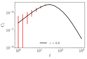
Figure 1: Angular power spectrum $C^{\rm HI}_{\ell}$ from at redshift 0.8, using the best-fitting HI astrophysical parameters from the halo model. The error bars shown in red represent the standard deviation $\Delta C^{\rm HI}_{l}$, calculated for a SKA 1 MID-like configuration.

An example angular power spectrum at $z\sim 0.8$ with its associated standard deviation (illustrated by the error bars) for a SKA I MID-like experimental configuration is shown in Fig. 1. The full Fisher matrix for an experiment is constructed by summing over the individual Fisher matrices in each of the $z$-bins in the range covered by the survey: $F_{ij,\rm cumul}=\sum_{z_{i}}F_{ij}(z_{i})$. Given the cumulative Fisher matrix, we can calculate the standard errors on the parameter $p_{i}$ for the cases of fixing and marginalizing over other parameters: $\sigma^{2}_{i,\rm fixed}=F_{ii}^{-1}$, and $\sigma^{2}_{i,\rm marg}=(F^{-1})_{ii}$. This is useful to quantify the degradation in cosmological constraints when astrophysical parameters are marginalized over. We find that (as shown in Fig. 2) although the astrophysical information broadens the cosmological constraints, the broadening is, for the large part, mitigated by the prior information coming from the present knowledge of the astrophysics, quantified by the halo model. We also find that experiments reaching lower $z$-values achieve more precise cosmological constraints, as do those having a larger tomographic coverage [such as the SKA I MID; Ref. 13].

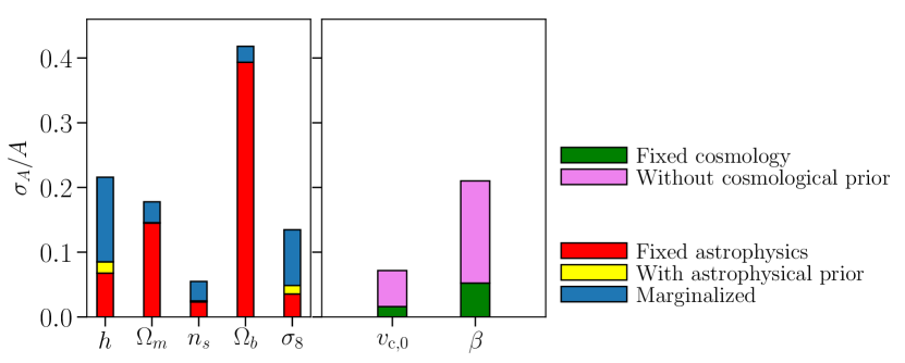
Figure 2: Left panel: Constraints on the cosmological parameters from a SKA I MID-like configuration, (i) marginalized over astrophysics, (ii) with fixed astrophysics, and (iii) with the astrophysical prior coming from the present data. Right panel: Astrophysical forecasts (i) without cosmological priors, and (ii) with fixed cosmology. Figure adapted from Ref. [13].

Cross-correlating 21 cm intensity maps with galaxy surveys (both photometric and spectroscopic) offers exciting prospects for constraining astrophysical and cosmological parameters. It can be shown [12] that cross-correlating such surveys covering similar redshift ranges and sky areas, significantly improves astrophysical constraints (see Fig. 3 for an example of a CHIME-like and DESI-like survey cross-correlated in the northern hemisphere). Further, cross-correlation is a valuable tool to mitigate the effects of contaminants and foregrounds, which are expected to be significantly uncorrelated between the two surveys [e.g., 2].

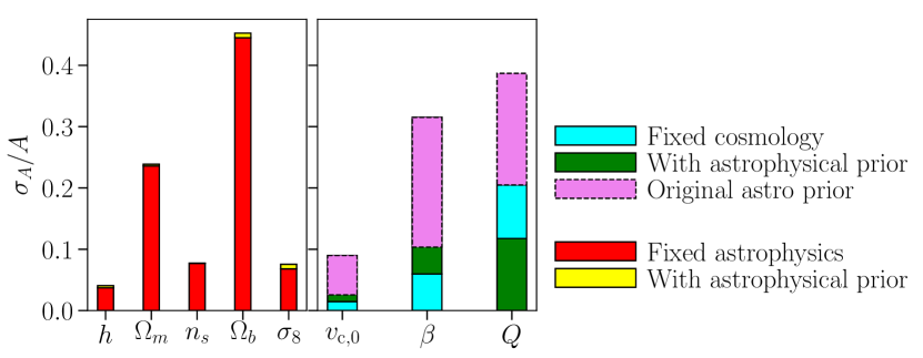
Figure 3: Cross-correlation forecasts for a CHIME-DESI like survey combination. Fractional errors, $\sigma_{A}/A$ are plotted for $A=\{h,\Omega_{m},n_{s},\Omega_{b},\sigma_{8},v_{c,0},\beta\}$, and an additional parameter $Q$ which quantifies the scale dependence of the optical galaxy bias. Left panel: Constraints on the cosmological parameters (i) without marginalizing over astrophysics, (ii) with the astrophysical prior coming from the present data. Right panel: Constraints on astrophysical parameters when: (i) not marginalizing over cosmology and (ii) marginalizing over cosmology and adding the astrophysical prior. The violet bands in the right panel show the extent of the prior in each case. Figure adapted from Ref. [12].

The Fisher formalism can also be used to quantify how a complementary effect, the accuracy of cosmological constraints, is affected by the astrophysical prior information. This can be done by calculating the relative biases on cosmological parameters, induced by a wrong assumption on the astrophysical ones. Such biases can be naturally quantified using the ‘nested likelihoods’ [e.g., 3] framework in which the parameter space is split into two subsets: one containing all the parameters of interest and the other, all those deemed ‘nuisance’ or systematic for the analysis being carried out. In the present case, these two sets represent ‘cosmological’ and ‘astrophysical’ parameters, respectively. The bias on a given cosmological parameter $p_{a}$, denoted by $b_{p_{a}}$, is computed as:

$$b_{p_{a}}=\delta p_{\alpha}F_{b\alpha}\left(\mathbf{F}^{-1}\right)_{ab}.$$ (11)

Here, $\mathbf{F}^{-1}$ is the full Fisher matrix of astrophysical and cosmological parameters, and $F_{b\alpha}$ represents the submatrix mixing cosmological and astrophysical parameters. The term $\delta p_{\alpha}$ denotes the vector of shifts in the astrophysical parameters from their fiducial values:

$$\delta p_{\alpha}=p_{\alpha}^{\rm fid}-p_{\alpha}^{\rm true}.$$ (12)

An exciting science case for current and future intensity mapping surveys lies in exploring effects beyond the standard model of $\Lambda$ CDM cosmology. Two widely-studied examples of beyond-$\Lambda$CDM physics include (i) the existence of a nonzero $f_{\rm NL}$ parameter that quantifies the primordial non-Gaussianity, and (ii) incorporating the effects of modified gravity by allowing the growth parameter, $\gamma$ to deviate from its fiducial value of 0.55. It can be shown [1] that these two effects lead to easily characterizable signatures on the intensity mapping power spectrum, by affecting the quantities $n_{h}(M)$ and $b_{h}(M,z)$, i.e. the abundance and bias of dark matter haloes. Thus, they can be incorporated in a straightforward manner into the angular power spectrum and as such, the Fisher forecasting formalism can be used to compute relative constraints on these observables in the presence of astrophysical uncertainties. Fig. 4 shows the relative biases on all the standard cosmological parameters, as well as $f_{\rm NL}$ and $\gamma$, induced by a deviation of either astrophysical parameter, $v_{\rm c,0}$ or $\beta$ from its fiducial (i.e. best-fit) value, as a function of the maximum multipole $\ell_{\rm max}$ considered in the analysis. The figure reveals that the relative biases on the standard cosmological parameters and the modified gravity parameter $\gamma$ all remain within a few $\sigma$ as long as the $\ell$ range stays below 1000. Remarkably, astrophysical uncertainties are found to have negligible effects on the $f_{\rm NL}$ parameter, despite it being strongly linked to the HI bias.

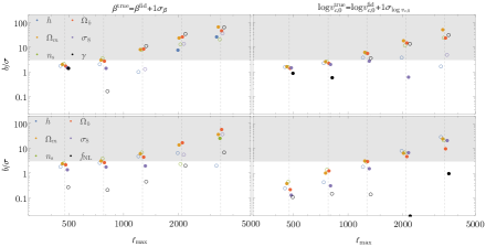
Figure 4: Relative bias on cosmological parameters in the extended-$\Lambda$CDM framework with a SKA I MID-like experimental configuration, obtained on shifting either astrophysical parameter, $\beta$ (left panels) or $\log v_{\rm c,0}$ (right panels), by $1\sigma$ from its fiducial value. Top panels contain the parameters in $\Lambda$CDM+$\gamma$, and lower panels contain those in $\Lambda$CDM+$f_{\rm NL}$. Empty (filled) circles indicate negative (positive) values of biases. Figure from Ref. [1].

3 Conclusions

In this article, we have explored the ability of current and future intensity mapping surveys to provide stringent constraints on cosmology and fundamental physics. A data-driven, halo model framework is well-positioned to mitigate the ‘astrophysical systematic’ effect on the precision and accuracy of cosmological forecasts from these surveys. Such an approach is a powerful tool to test extensions to the $\Lambda$CDM framework, such as primordial non-Gaussianity and deviations from General Relativity at cosmic scales, as well as to mitigate foregrounds through cross-correlating future intensity mapping and optical galaxy surveys. In the future, combining these datasets with more traditional probes of the high-redshift universe has the potential to uncover fundamental physics constraints from the hitherto unexplored epochs of Cosmic Dawn and reionization.

References

- [1] Camera, S., Padmanabhan, H.: Beyond CDM with HI intensity mapping: robustness of cosmological constraints in the presence of astrophysics. arXiv e-prints arXiv:1910.00022 (2019)
- [2] Cunnington, S., Wolz, L., Pourtsidou, A., Bacon, D.: Impact of Foregrounds on HI Intensity Mapping Cross-Correlations with Optical Surveys. arXiv e-prints arXiv:1904.01479 (2019)
- [3] Heavens, A.F., Kitching, T.D., Verde, L.: On model selection forecasting, Dark Energy and modified gravity. Mon. Not. Roy. Astron. Soc. 380, 1029–1035 (2007). 10.1111/j.1365-2966.2007.12134.x
- [4] Kovetz, E.D., Breysse, P.C., Lidz, A., Bock, J., Bradford, C.M., Chang, T.C., Foreman, S., Padmanabhan, H., Pullen, A., Riechers, D., Silva, M.B., Switzer, E.: Astrophysics and Cosmology with Line-Intensity Mapping. arXiv e-prints arXiv:1903.04496 (2019)
- [5] Limber, D.N.: The Analysis of Counts of the Extragalactic Nebulae in Terms of a Fluctuating Density Field. ApJ117, 134 (1953). 10.1086/145672
- [6] Loeb, A., Wyithe, J.S.B.: Possibility of Precise Measurement of the Cosmological Power Spectrum with a Dedicated Survey of 21cm Emission after Reionization. Phys.Rev.Lett100(16), 161301 (2008). 10.1103/PhysRevLett.100.161301
- [7] Macciò, A.V., Dutton, A.A., van den Bosch, F.C., Moore, B., Potter, D., Stadel, J.: Concentration, spin and shape of dark matter haloes: scatter and the dependence on mass and environment. MNRAS378, 55–71 (2007). 10.1111/j.1365-2966.2007.11720.x
- [8] Padmanabhan, H.: Constraining the CO intensity mapping power spectrum at intermediate redshifts. MNRAS475, 1477–1484 (2018). 10.1093/mnras/stx3250
- [9] Padmanabhan, H.: Constraining the evolution of [C II] intensity through the end stages of reionization. MNRAS488(3), 3014–3023 (2019). 10.1093/mnras/stz1878
- [10] Padmanabhan, H., Refregier, A.: Constraining a halo model for cosmological neutral hydrogen. MNRAS464(4), 4008–4017 (2017). 10.1093/mnras/stw2706
- [11] Padmanabhan, H., Refregier, A., Amara, A.: A halo model for cosmological neutral hydrogen : abundances and clustering H i abundances and clustering. Mon. Not. Roy. Astron. Soc. 469(2), 2323–2334 (2017). 10.1093/mnras/stx979
- [12] Padmanabhan, H., Refregier, A., Amara, A.: Cross-correlating 21 cm and galaxy surveys: implications for cosmology and astrophysics. arXiv e-prints arXiv:1909.11104 (2019)
- [13] Padmanabhan, H., Refregier, A., Amara, A.: Impact of astrophysics on cosmology forecasts for 21 cm surveys. MNRAS485(3), 4060–4070 (2019). 10.1093/mnras/stz683
- [14] Santos, M.G., Cooray, A., Knox, L.: Multifrequency Analysis of 21 Centimeter Fluctuations from the Era of Reionization. ApJ625(2), 575–587 (2005). 10.1086/429857
- [15] Seehars, S., Paranjape, A., Witzemann, A., Refregier, A., Amara, A., Akeret, J.: Simulating the large-scale structure of HI intensity maps. JCAP3, 001 (2016). 10.1088/1475-7516/2016/03/001