Relativistic kinetic gases as direct sources of gravity

Abstract

We propose a new model for the description of a gravitating multi particle system, viewed as a kinetic gas. The properties of the (colliding or non-colliding) particles are encoded into a so-called one-particle distribution function, which is a density on the space of allowed particle positions and velocities, i.e. on the tangent bundle of the spacetime manifold. We argue that an appropriate theory of gravity, describing the gravitational field generated by a kinetic gas, must also be modeled on the tangent bundle. The most natural mathematical framework for this task is Finsler spacetime geometry. Following this line of argumentation, we construct a coupling between the kinetic gas and a recently proposed Finsler geometric extension of general relativity. Additionally, we explicitly show how the general covariance of the action of the kinetic gas on the tangent bundle leads to a novel formulation of its energy-momentum conservation in terms of its energy-momentum distribution tensor.

I Introduction

An ensemble of a large number of $P$ individual interacting and gravitating point particles can be described on several levels of accuracy and detail:

• The most precise description is to derive the trajectories for each individual particle from their mutual interactions directly, which in general is a too complex task to be accomplished in a reasonable amount of time and with a reasonable amount of computational effort.

• Instead of deriving the behaviour of all individual particles, one can consider them as a kinetic gas and describe their properties collectively, in terms of a so-called one-particle distribution function (1PDF). The 1PDF still contains the information about the velocity distribution of the different particles, but further information about each individual particle is averaged out.

• Averaging the 1PDF over the velocities of the multiple particle system leads to its description as a fluid.

The gravitational field generated by the particles is usually obtained on the level of least accuracy in the above list. The energy-momentum tensor of a fluid is derived as second moment of the 1PDF with respect to the velocities of the particles, which then sources the Einstein equations. The dynamics of the fluid itself are given by the Euler equations, which follow from the fact that the energy-momentum tensor must be covariantly constant.

Since the description of the $P$ particle system as a kinetic gas is more accurate and finer than its fluid description, the conjecture of this article is that the same is true for the description of the gravitational field generated by the $P$ particle system. One feature which for example would be taken into account in this way is the velocity distribution over the different gas particles. In the fluid description the velocity distribution is averaged out.

Technically the 1PDF is a function on the tangent bundle of spacetime, or in other words on the position and velocity space of the particles. It describes the number of particles in the gas and their trajectories. When averaged over the particle velocities, one can extract information about the pressure, density and energy-momentum of the resulting fluid description, see Israel ; Ehlers2011 and (Rezzolla2013, , Sec. 2.3), or Sarbach:2013fya . A geometric description of the kinetic gas and its dynamics on the tangent bundle has been investigated in Sarbach:2013uba and was applied to the formation of accretion discs in Rioseco:2016jwc . Moreover, first post Newtonian corrections to the behaviour of a gravitating gas in a fixed gravitational behaviour have been studied Agon:2011mz ; RamosCaro:2012rz . What is missing in these approaches is the dynamical backreaction of the kinetic gas on the gravitational field, accordingly a dynamical equation which determines the gravitational field generated by the kinetic gas directly.

The aim of this article is to present how a kinetic gas, in terms of the 1PDF, can be directly coupled to gravity, and how the 1PDF is the source term of a gravitational field equation directly on the tangent bundle.

In order to couple the 1PDF to gravity without averaging, it is necessary to construct the dynamics of the gravitational field on the same space on which the 1PDF lives. Since gravity is encoded into the geometry of spacetime, this implies that we need a description of the geometry of spacetime on the tangent bundle. A natural mathematical framework for this task is Finsler geometry Finsler ; Bucataru ; Shen .

The idea of using Finsler geometry as generalized geometry of spacetime has been considered in the literature for long Beem ; Pfeifer:2011tk ; Javaloyes:2018lex ; Asanov ; Bucataru ; Goenner:2008rr ; Hohmann:2018rpp . Simultaneously, multiple attempts of finding Finsler generalisations of the Einstein equations have been made Asanov ; Rutz ; Li2014 ; Pfeifer ; Hohmann:2018rpp ; Minguzzi:2014fxa . Besides mathematical difficulties in the precise consistent formulation of indefinite Lorentzian Finsler geometry, one most important open question, in all of the attempts of using Finsler geometry as physically viable extension of the geometry of spacetime, is how to couple the geometry to physical matter fields correctly. One particular obstacle is that a Finslerian geometry does not only depend on the points of spacetime, but also on its directions.

By studying the kinetic gas in the language of Finsler geometry, we turn this obstacle into an advantage. Extending the previous studies Hohmann:2015ywa ; Hohmann:2015duq , which considered the dynamics of a kinetic gas in Finsler geometric language in the context of cosmology, we formulate an action of the kinetic gas on the tangent bundle. Its general covariance, i.e. invariance under coordinate changes of the base manifold, yields a new formulation of energy-momentum conservation of a kinetic gas in terms of a quantity directly formulated on the tangent bundle - the energy-momentum distribution tensor - and it enables us to couple the gas to gravity in a simple way. The Finslerian extension of Einstein gravity which was proposed in Pfeifer , and further developed to mathematical rigour and consistency recently Hohmann:2018rpp , provides the canonical gravitational field equation on the tangent bundle, which naturally can be sourced by the 1PDF. By constructing the coupling of a kinetic gas to the Finslerian geometry of spacetime explicitly, we demonstrate how physically viable matter leads to a Finslerian spacetime geometry dynamically and solve the problem of how to couple physical matter to a Finsler geometric theory of gravity.

The future application of the gravitational field equation is expected to highly improve the understanding of systems that are described by gravitating fluids, such as the universe as a whole in cosmology, ordinary and neutron stars, as well as accretion disks of black holes, by replacing the averaged gravitating fluid by the more accurate and finer notion of a kinetic gas.

We present our results as follows. In Section II we recapitulate the main mathematical notions of Finsler spacetime geometry, which are necessary to describe the kinetic gas in terms of Finsler geometry in Section III. The definition of the 1PDF is provided in Section III.1. Then we use the 1PDF to construct an action of the kinetic gas on the tangent bundle in Section III.2, before we find the energy-momentum distribution tensor of the kinetic gas from the general covariance of the action in Section III.3. Finally, in Section IV we derive the Finsler gravitational field equations coupled to the kinetic gas before we conclude in Section V.

II The geometric setup

The stage on which we couple the kinetic gas to gravity is the tangent bundle $TM$ of a spacetime manifold $M$, which we assume to be of dimension $4$ here. However, the whole construction presented in this article can straightforwardly be generalized to any spacetime dimension. Any local coordinate chart $(U,x^{a})$ on $M$ induces a local coordinate chart $(TU,(x^{a},\dot{x}^{a}))$ on $TM$, where an element $\dot{x}\in TU$ is a vector $\dot{x}$ in some tangent space $T_{x}M,x\in U$, which in local coordinates can be expressed as $\dot{x}=\dot{x}^{a}\partial_{a}|_{x}$. This procedure associates the manifold induced coordinates $(x^{a},\dot{x}^{a})$ to $\dot{x}$. If there is no risk of confusion, we will sometimes omit the indices in the coordinate representation. The canonical coordinate basis of the tangent and cotangent spaces of $TM$ is denoted by $(\partial_{a}=\frac{\partial}{\partial x^{a}},\dot{\partial}_{a}=\frac{\partial}{\partial\dot{x}^{a}})$ resp. $(dx^{a},d\dot{x}^{a})$.

II.1 Finsler spacetimes

To describe the kinetic gas and its coupling to gravity geometrically on the tangent bundle, we employ Finsler spacetime geometry and the Finsler spacetime geometric description of the gravitational dynamics Hohmann:2018rpp ; Pfeifer:2019wus ; Pfeifer:2011tk ; Pfeifer .

The Finslerian geometry of spacetime is derived from the geometric clock of observers, resp. free point particle action for massive particles on trajectories $\gamma:\mathbb{R}\rightarrow M,\tau\mapsto\gamma(\tau)$, with tangent vectors denoted by $\dot{\gamma}=\frac{\partial\gamma^{a}}{\partial\tau}\partial_{a}=\dot{\gamma}^{a}\partial_{a}$ and tangent bundle representation $(\gamma,\dot{\gamma})$:

$$S[\gamma]=\int d\tau\ F(\gamma,\dot{\gamma})\,,$$ (1)

where $F$ is a $1$-homogeneous function on $TM$ with respect to its second argument. Later, when we consider the relativistic kinetic gas in Section III, we assume that the trajectories $\gamma(\tau)$ of the particles which constitute the gas extremize this length functional, i.e. they are the geodesics of (1).

To make the mathematical setup precise, we recall the definition of Finsler spacetimes with which we work here. Details about this definition can be found in Hohmann:2018rpp , which was distilled from existing definitions in the literature Javaloyes:2018lex ; Lammerzahl:2012kw ; Beem .

Definition 1

Let $\mathcal{A}$ be a conic subbundle of $TM$ such that $TM\setminus\mathcal{A}$ is of measure zero. A Finsler spacetime is a pair $(M,L)$, where $L:\mathcal{A}\rightarrow\mathbb{R}$ is a smooth function, called the Finsler-Lagrange function, which satisfies:

• $L$ is positively homogeneous of degree two with respect to $\dot{x}$: $L(x,\alpha\dot{x})=\alpha^{2}L(x,\dot{x}),\ \alpha\in\mathbb{R}^{+}$;

• on $\mathcal{A}$ the vertical Hessian

  $$g^{L}_{ab}=\dfrac{1}{2}\dfrac{\partial^{2}L}{\partial\dot{x}^{a}\partial\dot{x}^{b}}$$ (2)

  of $L$ (called $L$-metric) is non-degenerate in every coordinate chart;

• there exists a connected component $\mathcal{T}$ of the preimage $L^{-1}((0,\infty))\subset TM$ on which $g^{L}$ exists, is smooth and has Lorentzian signature $(+,-,-,-)~{}$

• the Euler-Lagrange equations

  $$\frac{d}{d\tau}\dot{\partial}_{a}L-\partial_{a}L=0\,.$$ (3)

  have a unique local solution for every initial condition $(x,\dot{x})\in\mathcal{T}\cup\mathcal{N}$, where $\mathcal{N}$ is the kernel of $L$. At points of $\mathcal{N}\setminus\mathcal{A}$, i.e. where the $L$-metric degenerates or does not even exist, the solution must be constructed by continuous extension. This means that the geodesic equation coefficients admit a $\mathcal{C}^{1}$ extension at those points.

The $1$-homogeneous function $F$, which defines the point particle action (1), is derived from the Finsler Lagrange function as $F=\sqrt{|L|}$. For clarity, we list the different sets which appear in the definition and comment on their meaning:

• $\mathcal{A}$: the subbundle where $L$ is smooth and $g^{L}$ is non-degenerate, with fiber $\mathcal{A}_{x}=\mathcal{A}\cap T_{x}M$, called the set of admissible vectors,

• $\mathcal{N}$: the subbundle where $L$ is zero, with fiber $\mathcal{N}_{x}=\mathcal{N}\cap T_{x}M$,

• $\mathcal{A}_{0}=\mathcal{A}\setminus\mathcal{N}$: the subbundle where $L$ can be used for normalization, with fiber $\mathcal{A}_{0x}=\mathcal{A}_{0}\cap T_{x}M$,

• $\mathcal{T}$: a maximally connected conic subbundle where $L>0$, the $L$-metric exists and has Lorentzian signature $(+,-,-,-)$, with fiber $\mathcal{T}_{x}=\mathcal{T}\cap T_{x}M$.

The connected component $\mathcal{T}$ is interpreted as the set of future directed timelike directions on spacetime. An important subset of the timelike directions is formed by the future pointing unit timelike vectors

$$\mathcal{O}:=\{(x,\dot{x})\in\mathcal{T}|L(x,\dot{x})=1\}\,,$$ (4)

which is called the observer space Gielen:2012pn ; Gielen:2012fz ; Hohmann:2013fca ; Hohmann:2014gpa ; Hohmann:2015pva . This set is itself a fibered manifold over $M$, with fibers $\mathcal{O}_{x}=\mathcal{O}\cap T_{x}M$.

Finsler spacetimes are a straightforward generalisation of pseudo-Riemannian spacetimes equipped with a metric $g_{ab}$ of Lorentzian signature. The latter constitute a subclass of Finsler spacetimes $(M,L)$ with $L=g_{ab}(x)\dot{x}^{a}\dot{x}^{b}$, defined by the components of a pseudo-Riemannian metric.

II.2 Geometry of Finsler spacetimes

Finsler geometry is a long-standing straightforward generalisation of Riemannian geometry Shen ; Bucataru . Finsler spacetime geometry is, up to the precise definition of Finsler spacetimes, an equally straightforward generalisation of pseudo-Riemannian geometry. Here we recall the geometric notions we need to describe the kinetic gas consistently in the language of Finsler geometry and to couple it as source term to the Finsler gravitational field equation.

Starting from the Finsler Lagrange function $L$, we can define canonical tensor fields on $\mathcal{A}_{0}\subset TM$. The Hilbert form $\omega$, the Finsler metric tensor $g^{L}$ and the Cartan tensor $C$, using the notation $\dot{x}_{a}=g^{L}_{ab}(x,\dot{x})\dot{x}^{b}$, are,

$$\omega=\dot{\partial}_{a}Fdx^{a}=\frac{L}{|L|}\frac{\dot{x}_{a}}{\sqrt{|L|}}dx^{a},\quad g^{L}=g^{L}_{ab}dx^{a}\otimes dx^{b},\quad C=\frac{1}{2}\dot{\partial}_{c}g^{L}_{ab}dx^{a}\otimes dx^{b}\otimes dx^{c}\,.$$ (5)

The geodesic equations of (1) in arc length parametrization are given by the Euler-Lagrange equations (3) and take the form

$$\ddot{x}^{a}+2G^{a}(x,\dot{x})=0\,.$$ (6)

They are defined in terms of the so-called spray coefficients $G^{a}$, which in turn determine the Cartan non-linear connection coefficients $G^{a}{}_{b}$

$$G^{a}=\frac{1}{4}g^{Lab}\left(\dot{x}^{m}\partial_{m}\dot{\partial}_{b}L-\partial_{b}L\right),\quad G^{a}{}_{b}:=\dot{\partial}_{b}G^{a}\,.$$ (7)

The connection coefficients give rise to a splitting of the tangent and cotangent spaces to $\mathcal{A}$, into so-called horizontal and vertical parts. Locally, they are spanned by the basis vector fields

$$T_{(x,\dot{x})}\mathcal{A}=\textrm{span}\{\delta_{a}=\partial_{a}-G^{b}{}_{a}\dot{\partial}_{b};\ \dot{\partial}_{a}\}_{a=0}^{3}\,,\quad T^{*}_{(x,\dot{x})}\mathcal{A}=\textrm{span}\{dx^{a};\ \delta\dot{x}^{a}=dx^{a}+G^{a}{}_{b}d\dot{x}^{b}\}_{a=0}^{3}\,.$$ (8)

With help of this adapted basis, on $\mathcal{A}_{0}$ we can introduce the following vector field, which is dual to the Hilbert form,

$$\mathbf{r}=\frac{\dot{x}^{a}}{\sqrt{|L|}}\delta_{a},\quad\mathbf{i}_{\mathbf{r}}\omega=\omega(\mathbf{r})=1\,.$$ (9)

The restriction of $\mathbf{r}$ to the observer space $\mathcal{O}$ is called the Reeb vector field $\mathbf{r}|_{\mathcal{O}}$ associated to $\omega$. By Cartan’s magic formula, which relates the interior product, the exterior derivative and the Lie derivative $\mathfrak{L}_{X}=\mathbf{i}_{X}d+d\mathbf{i}_{X}$, and by the explicit expansion of $d\omega$ in the adapted basis the following important relation is satisfied

$$\mathfrak{L}_{\mathbf{r}}\omega=\mathbf{i}_{\mathbf{r}}d\omega+d\mathbf{i}_{\mathbf{r}}\omega=\mathbf{i}_{\mathbf{r}}d\omega=0\,.$$ (10)

The curvature tensor $\mathfrak{R}$ of the Cartan non-linear connection and the Finsler Ricci scalar $R_{0}$ are defined as

$$\mathfrak{R}=\frac{1}{2}R^{a}{}_{bc}dx^{b}\wedge dx^{c}\otimes\dot{\partial}_{a},\quad R^{a}{}_{bc}\dot{\partial}_{a}=(\delta_{b}G^{a}{}_{c}-\delta_{c}G^{a}{}_{b})\dot{\partial}_{a}=[\delta_{b},\delta_{c}],\quad R_{0}=\frac{1}{L}R^{a}{}_{ab}\dot{x}^{b}\,.$$ (11)

Last but not least, the canonical volume form on the set $\mathcal{A}_{0}$ of a Finsler spacetime is given by

$$\textrm{Vol}_{0}=\frac{|\det g^{L}|}{L^{2}}d^{4}x\wedge d^{4}\dot{x}:=\frac{|\det g^{L}|}{L^{2}}dx^{0}\wedge...\wedge dx^{3}\wedge d\dot{x}^{0}\wedge...\wedge d\dot{x}^{3}\,.$$ (12)

Denote by $\mathbb{C}=\dot{x}^{a}\dot{\partial}_{a}$ the Liouville vector field. It gives rise to a $7$-form $\Sigma$, see also Hohmann:2018rpp ,

$$\Sigma =\mathbf{i}_{\mathbb{C}}\textrm{Vol}_{0}=\frac{1}{3!}\omega\wedge d\omega\wedge d\omega\wedge d\omega=\frac{|\det g^{L}|}{L^{2}}\mathbf{i}_{\mathbb{C}}(d^{4}x\wedge d^{4}\dot{x})$$ (13)

$$=\frac{1}{3!}\frac{|\det g^{L}|}{L^{2}}\dot{x}^{a}\epsilon_{abcd}dx^{0}\wedge...\wedge dx^{3}\wedge d\dot{x}^{b}\wedge d\dot{x}^{c}\wedge d\dot{x}^{d}\,,$$ (14)

and a $6$-form $\Omega$

$$\Omega=\mathbf{i}_{\mathbf{r}}\Sigma=\frac{1}{3!}d\omega\wedge d\omega\wedge d\omega\,,$$ (15)

which obey

$$d\Omega=0,\quad\Sigma=\omega\wedge\Omega\,.$$ (16)

These differential forms will play the role of canonical volume forms on different subsets of the observer space $\mathcal{O}$.

In the literature on Finsler geometry several canonical linear covariant derivatives on $TM$ are considered, which all reduce to the Levi-Civita connection in the case of Pseudo-Riemannian geometry, i.e. , Finsler geometry with a Finsler Lagrangian that is quadratic in the dependence on $\dot{x}$, i.e. $L=g_{ab}(x)\dot{x}^{a}\dot{x}^{b}$. We employ the so called Chern-Rund linear covariant derivative, which can be defined by its action in the adapted basis as

$$\nabla_{\delta_{a}}\delta_{b}=\Gamma^{c}{}_{ab}\delta_{c},\ \nabla_{\delta_{a}}\dot{\partial}_{b}=\Gamma^{c}{}_{ab}\dot{\partial}_{c},\ \nabla_{\dot{\partial}_{a}}\delta_{b}=0,\ \nabla_{\dot{\partial}_{a}}\dot{\partial}_{b}=0\,,$$ (17)

with $\Gamma^{c}{}_{ab}=\frac{1}{2}g^{Lcq}(\delta_{a}g^{L}_{bq}+\delta_{b}g^{L}_{aq}-\delta_{q}g^{L}_{ab})$. It satisfies the important identities, see (Bucataru, , p.104),

$$\nabla_{\delta_{a}}\dot{x}^{b}=0,\nabla_{\delta_{a}}L=0\textrm{ and }\nabla_{\delta_{a}}g^{L}{}_{bc}=0\,,$$ (18)

which we prove for completeness in Appendix A. Furthermore there exists the so-called dynamical covariant derivative, which is uniquely defined in terms of the canonical Cartan non-linear connection alone, independently of the choice of linear connection; we denoted the dynamical covariant derivative by $\nabla$ without any index. Operationally, it can be understood as

$$\nabla\delta_{b}:=\dot{x}^{a}\nabla_{\delta_{a}}\delta_{b}=G^{c}{}_{b}\delta_{c},\ \nabla\dot{\partial}_{b}=\dot{x}^{a}\nabla_{\delta_{a}}\dot{\partial}_{b}=G^{c}{}_{b}\dot{\partial}_{c}\,.$$ (19)

Last but not least, we recall the components of the Landsberg tensor, in terms of the connection coefficients of the Chern-Rund connection or equivalently with help of the dynamical covariant derivative of the Cartan tensor,

$$P^{a}{}_{bc}=\dot{\partial}_{c}G^{a}{}_{b}-\Gamma^{a}{}_{cb}=g^{Lad}\nabla C_{dbc}\,.$$ (20)

The trace $P_{b}=P^{a}{}_{ab}$ will be part of the geometry side of the gravitational field equation (56).

With the help of the geometric setup just introduced, we can now describe a relativistic kinetic gas.

III The kinetic gas in the language of Finsler geometry

Instead of describing a relativistic gas, i.e. a collection of relativistic particles, particle by particle, the kinetic gas theory employs a 1PDF to describe the gas particles collectively. This approach to the description of the gas is more accurate than its approximation as a fluid. Classical reference to the topic are the article by Israel Israel and the lectures by Ehlers Ehlers2011 . A modern review can be found in the monograph Rezzolla2013 or in the articles Sarbach:2013fya ; Sarbach:2013uba .

In terms of the 1PDF, kinetic gases are naturally described on the tangent bundle of a manifold, which is the same stage on which Finsler geometry naturally lives. In this section, we introduce the 1PDF and use the geometry of Finsler spacetimes to deduce the action of a kinetic gas on the observer space $\mathcal{O}$ over $M$. Moreover, we study the conservation laws which follow from the invariance of the action under arbitrary 1-parameter groups of spacetime induced coordinate changes on $TM$. The arising Noether currents point out the novel notion of an energy-momentum distribution tensor of the gas on the tangent bundle, via a Gotay-Marsden type procedure GotayMarsden ; Voicu:EM . We will relate this new notion of energy-momentum to the usual definition of the energy-momentum tensor of a kinetic gas on the spacetime manifold $M$.

The analysis of the properties of the tangent bundle action of a kinetic gas prepares its coupling to Finsler gravity in the next section.

III.1 General description

A kinetic gas is a collection of $P$ particles which propagate through spacetime on piecewise normalized geodesics $\gamma(\tau)$. In the language of a Finsler spacetime, this means that the tangent vectors of the trajectories of particles are elements of the observer space, $\frac{d\gamma}{d\tau}=\dot{\gamma}(\tau)\in\mathcal{O}_{\gamma(\tau)}\subset\mathcal{T}_{\gamma(\tau)}$ and that the tangents of the lifted trajectories $c(\tau)=(\gamma(\tau),\dot{\gamma}(\tau))$ are given by the Reeb vector field $\dot{c}=\mathbf{r}|_{c}$. The latter statement is equivalent to saying that the particle trajectories extremize the point particle action integral

$$S[\gamma]=m\int_{\tau_{1}}^{\tau_{2}}c^{*}\omega=m\int_{\tau_{1}}^{\tau_{2}}\frac{\dot{\gamma}_{a}}{\sqrt{|L(\gamma,\dot{\gamma})|}}c^{*}(dx^{a})=m\int_{\tau_{1}}^{\tau_{2}}\frac{\dot{\gamma}_{a}}{\sqrt{|L(\gamma,\dot{\gamma})|}}\dot{\gamma}^{a}d\tau=m\int_{\tau_{1}}^{\tau_{2}}d\tau\ F(\gamma,\dot{\gamma})=mt\,.$$ (21)

It is defined by a Finsler function $F$, which in turn is derived from a Finsler spacetime Lagrange function $L$, see Definition 1. The number $t=\tau_{2}-\tau_{1}$ denotes the proper time passing along a particle trajectory between $\gamma(\tau_{1})$ and $\gamma(\tau_{2})$.

Instead of describing the motion of all particles individually, the kinetic gas theory employs the 1PDF,

$$\phi:\mathcal{O}\rightarrow\mathbb{R};\quad(x,\dot{x})\mapsto\phi(x,\dot{x})\,,$$ (22)

which expresses the number $N[\sigma]$ of particle trajectories passing through an oriented, 6-dimensional hypersurface $\sigma\subset\mathcal{O}$ through the integral

$$N[\sigma]=\int_{\sigma}\phi\Omega\,.$$ (23)

It vanishes for hypersurfaces for which the tangent vectors $\dot{c}$ are tangent to $\sigma$, i.e. $\dot{c}\in T_{c}\sigma$. The integral is non-vanishing for hypersurfaces that are transversal to the particle trajectories, i.e. for which $\dot{c}\notin T_{c}\sigma$. The canonical volume form $\Omega$ on $\sigma$ was defined in (13). Since in all practical physical situations, there will always be gas particles with a finite maximal velocity, we assume in what follows that for all $x\in M$ $\phi_{x}(\dot{x})=\phi(x,\dot{x})$ has compact support on the set of future pointing unit timelike directions $\mathcal{O}_{x}$.

An important feature of this integral is that its result is independent of the geometric field $L$ on $TM$. It only depends on the trajectories of the particles and the hypersurface chosen. Therefore, its variation with respect to the Finsler Lagrangian vanishes and we find the equation

$$\delta_{L}N[\sigma]=\int_{\sigma}\delta_{L}(\phi\ \Omega)=\int_{\sigma}(\delta_{L}\phi\Omega+\phi\delta_{L}\Omega)=0\,.$$ (24)

It defines a relation between the 1PDF $\phi$ and the Finsler Lagrangian $L$, which is the important feature that couples the gas to the geometry of spacetime.

For a collisionless gas, the Liouville equation holds

$$\mathbf{r}(\phi)=\dot{x}^{a}\delta_{a}\phi=0\,,$$ (25)

which can be seen by the following argument, see for example Sarbach:2013fya ; Hohmann:2015ywa . Choose a hypersurface $\sigma_{0}\subset\mathcal{O}$ as above. We obtain a family of hypersurfaces $\sigma_{s}$ by following the flow of the Reeb vector field $\mathbf{r}$ from each point in $\sigma_{0}$ for one and the same parameter $0<s<t$. This family of hypersurfaces spans a volume $V=\bigcup_{s\in(0,t)}\sigma_{s}$, see Figure 1 for a sketch.

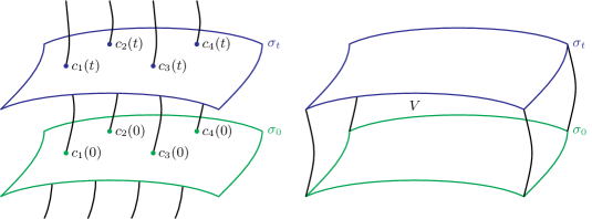
Figure 1: Construction of hypersurfaces by the flow of the Reeb vector field, and the corresponding swept out volume.

The difference between the number of particles on $\sigma_{0}$ and $\sigma_{t}$ is given by

$$N[\sigma_{t}]-N[\sigma_{0}]=\int_{V}\mathbf{r}(\phi)\ \Sigma\,.$$ (26)

For a collisionless gas $N[\sigma_{t}]-N[\sigma_{0}]=0$ and hence the Liouville equation (25) follows. The proof of (26) involves Stokes’ Theorem and the properties (16) of the forms $\Omega$ and $\Sigma$, details can be found in Sarbach:2013fya ; Hohmann:2015ywa .

With help of the 1PDF and the number counting integral, we can now construct the action of a kinetic gas on $TM$.

III.2 The action of a kinetic gas

Let us consider a kinetic gas which consists of $P$ individual particles of equal mass $m$. Hence the action of a gas in a volume $V$ generated by the flow of the Reeb vector field from an initial hypersurface $\sigma_{0}$, which is pierced by all $P$ particle trajectories, to a final hypersurface $\sigma_{t}$, with flow parameter $0\leq s\leq t$, $V=\bigcup_{0<s<t}\sigma_{s}\subset U$, see Figure 1, is given by

$$S_{\text{gas}}=mPt=mP\int_{\tau_{1}}^{\tau_{2}}d\tau\ F(\gamma,\dot{\gamma})=P\int_{\tau_{1}}^{\tau_{2}}c^{*}\omega=m\int_{0}^{t}Pds\,.$$ (27)

To express the action in terms of the 1PDF, we will express the particle number $P$ in (27) by the number counting integral $P=N[\sigma_{s}]$ to obtain

$$S_{\text{gas}}=m\int_{0}^{t}\left(\int_{\sigma_{s}}\phi\Omega\right)ds=m\int_{V}\phi\Omega\wedge\omega\,.$$ (28)

Applying the relation (16), which relates the different volume forms, we conclude that the tangent bundle action of a kinetic gas is

$$S_{\text{gas}}=m\int_{V}\phi\Sigma\,.$$ (29)

This action depends on the particle trajectories $(\gamma(\tau),\dot{\gamma}(\tau))$, which determine the 1PDF $\phi(x,\dot{x})$ from the number integral (23), and on the geometry defining Finsler Lagrange function $L$. It thus is defined by the Lagrangian $7$-form

$$\lambda(x,\dot{x},L(x,\dot{x}),\dot{\partial}\dot{\partial}L(x,\dot{x}))=m\phi\Sigma\,.$$ (30)

Variation of the action with respect to the particle trajectories yields the Finsler geodesic equation for each of the particles, while variation with respect to the Finsler Lagrange function yields the source term for the gravitational dynamics.

We like to remark that the volume $V$ over which the action integral is taken is usually assumed to be composed out of compact domains $D\subset M$ and $V_{x}\subset\mathcal{O}_{x}$ for each $x\in D$, where $V_{x}$ is chosen such that it contains the support of $\phi_{x}$, i.e. $V=\bigcup_{x\in D}V_{x}$. With such choice of $V$, it is possible to split the action integral

$$S_{\text{gas}}=m\int_{V}\phi\Sigma=m\int_{D}\left(\int_{V_{x}}\phi_{x}(\dot{x})\Sigma_{x}\right)d^{4}x=m\int_{D}\left(\int_{\mathcal{O}_{x}}\phi_{x}(\dot{x})\Sigma_{x}\right)d^{4}x\,,$$ (31)

where $\Sigma_{x}$ is the volume measure on $\mathcal{O}_{x}$ obtained from $\Sigma_{x}=\mathbf{i}_{\partial_{0}}\mathbf{i}_{\partial_{1}}\mathbf{i}_{\partial_{2}}\mathbf{i}_{\partial_{3}}\Sigma=\frac{\det g^{L}}{L^{2}}\mathbf{i}_{\mathbb{C}}(d^{4}\dot{x})$. The extension of the integration from $V_{x}$ to $\mathcal{O}_{x}$ is always possible by the assumption of compact support of $\phi_{x}$.

Before we investigate the gravitational dynamics sourced by the kinetic gas in Section IV, we now deduce the energy-momentum of the gas on the tangent bundle from manifold induced coordinate invariance of the action $S_{\text{gas}}$.

III.3 General covariance and energy-momentum conservation

All geometric objects in Finsler geometry have a distinguished behaviour under coordinate changes of the base manifold. That means even though the objects introduced in Section II.2 are objects on the tangent bundle, their components in the adapted basis transform under coordinate changes of $TM$ induced by coordinate changes of $M$ just as if they were objects on $M$.

More precisely, consider a local coordinate change $x^{a}\mapsto\tilde{x}^{a}(x)$ on $M$. Such a coordinate change naturally induces a local coordinate change on $TM$ by $(x^{a},\dot{x}^{a})\mapsto(\tilde{x}^{a},\dot{\tilde{x}}^{a})=(\tilde{x}^{a}(x),\frac{\partial\tilde{x}^{a}}{\partial x^{b}}(x)\dot{x}^{b})$. The basis change of the adapted horizontal and vertical bases are

$$\tilde{\delta}_{a}=\tilde{\partial}_{a}x^{b}\delta_{b},\ \dot{\tilde{\partial}}_{a}=\tilde{\partial}_{a}x^{b}\dot{\partial}_{b},\quad d\tilde{x}^{a}=\partial_{b}\tilde{x}^{a}dx^{b},\ \delta\tilde{\dot{x}}^{a}=\partial_{b}\tilde{x}^{a}\delta\dot{x}^{b}\,.$$ (32)

Since all Finsler geometric objects are naturally expressed in the adapted basis, their components transform under manifold induced coordinate changes precisely the same way. All tensor fields on $TM$ with this property, are called $d$-, or distinguished, tensor fields, see Bucataru ; Hohmann:2018hac for details on d-tensors.

Since the Lagrangian $7$-form of the kinetic gas $\lambda=m\phi\Sigma$ is constructed out of a scalar and Finsler geometric objects, it is a $d$-$7$-form, and hence invariant under manifold induced coordinate changes. Studying infinitesimal manifold induced coordinate changes gives rise to conserved currents and an energy-momentum tensor of the gas on $TM$, which we will call energy-momentum distribution tensor $\Theta$. It will turn out that this new tangent-bundle notion of energy-momentum distribution tensor of a kinetic gas is related to the usual definition of its energy-momentum tensor on the base manifold by averaging.

Infinitesimal manifold induced coordinate changes, labelled with a small expansion parameter $\epsilon$, are generated by a vector field $\xi=\xi^{a}(x)\partial_{a}$

$$\tilde{x}^{a}(x)=x^{a}+\epsilon\xi^{a}\,.$$ (33)

The corresponding manifold induced coordinate change on $TM$ is given by the additional change

$$\dot{\tilde{x}}^{a}(x,\dot{x})=\dot{x}^{a}+\epsilon\dot{x}^{b}\partial_{b}\xi^{a}\,.$$ (34)

Hence the total infinitesimal coordinate change on $TM$ is induced by the complete lift $\xi^{C}=\xi^{a}(x)\partial_{a}+\dot{x}^{b}\partial_{b}\xi^{a}\dot{\partial}_{a}$ of the vector field $\xi$. In the adapted basis $\xi^{C}=\xi^{a}\delta_{a}+\nabla\xi^{a}\dot{\partial}_{a}$ holds.

The Lagrangian $7$-form depends on the coordinates on $TM$ and on the field variable $L$. Hence its variation can be written as

$$\delta_{\xi}\lambda(x,\dot{x},L,\dot{\partial}\dot{\partial}L)=\frac{d}{d\epsilon}\lambda(x+\epsilon\delta x,\dot{x}+\epsilon\delta\dot{x},L+\epsilon\delta L,\dot{\partial}\dot{\partial}L+\epsilon\dot{\partial}\dot{\partial}\delta L)|_{\epsilon=0}\,,$$ (35)

where $\delta x^{a}=\xi^{a},\ \delta\dot{x}^{a}=\dot{x}^{b}\partial_{b}\xi^{a}$ and $\delta L=-\xi^{C}(L)$. Evaluating the above derivative carefully, as it is done in Appendix B, yields the expression

$$\delta_{\xi}\lambda=m\left(\mathfrak{L}_{\xi^{C}}(\phi\Sigma)+\delta_{L}(\phi\Sigma)\delta L\right)\,.$$ (36)

Using Cartan’s magic formula $\mathfrak{L}_{X}=\mathbf{i}_{\xi^{C}}d+d\mathbf{i}_{\xi^{C}}$ in the first terms in (36) reveals the equality

$$\mathfrak{L}_{\xi^{C}}(\phi\Sigma) =\mathbf{i}_{\xi^{C}}d(\phi\Sigma)+d\mathbf{i}_{\xi^{C}}(\phi\Sigma)=d\mathbf{i}_{\xi^{C}}(\phi\Sigma)\,,$$ (37)

where the term $\mathbf{i}_{\xi^{C}}d(\phi\Sigma)$ vanishes since $\Sigma$ is a form of maximal rank on $\mathcal{O}$ and thus $d(\phi\Sigma)=0$.

The second term in (36) gives

$$\delta_{L}(\phi\Sigma)\delta L =(\delta_{L}(\phi\Omega)\wedge\omega+\phi\Omega\wedge\delta_{L}\omega)\delta L$$

$$=(\phi\Omega\wedge\delta_{L}\omega)\delta L$$

$$=\frac{1}{2L}\phi\ \delta L\ \Sigma$$ (38)

$$=-\frac{1}{2L}\phi\ \xi^{C}(L)\ \Sigma=-\frac{1}{2L}\phi\ \dot{\partial}_{a}L\nabla\xi^{a}\ \Sigma\,.$$ (39)

In the first line we used $\Sigma=\Omega\wedge\omega$ and in the second line that $\delta_{L}(\phi\Omega)=0$, see (24). To reach the third line, the derivation of $\Omega\wedge\delta_{L}\omega=\frac{1}{2L}\phi\Sigma$ as it is displayed in Appendix C was applied. Finally, for the variation with respect to the manifold induced coordinates, we have that $\delta L=-\xi^{C}(L)=\nabla\xi^{a}\dot{\partial}_{a}L$, since $\delta_{a}L=0$. Inserting $\dot{\partial}_{a}L=2g^{L}_{ab}(x,\dot{x})\dot{x}^{b}=2\dot{x}_{a}$, the total change of the Lagrange $7$-form of the kinetic gas is given by

$$\delta_{\xi}\lambda=m\left(-\phi\frac{\dot{x}_{a}}{L}\nabla\xi^{a}\ \Sigma+d\mathbf{i}_{\xi^{C}}(\phi\Sigma)\right)\,,$$ (40)

and so the variation of the action is

$$\delta_{\xi}S_{\text{gas}}=-m\int_{V}\phi\frac{\dot{x}_{a}}{L}\nabla\xi^{a}\ \Sigma+m\int_{\partial V}\mathbf{i}_{\xi^{C}}(\phi\Sigma)\,.$$ (41)

From equation (38) we see that the integrand of the volume integral in (41) is the Euler-Lagrange part of the variation of the action with respect to the Finsler Lagrange function $L$, which will define the source term of the gravitational dynamics in the next section. The boundary term, where $\partial V=(\bigcup_{x\in D}\partial V_{x})\cup(\bigcup_{x\in\partial D}V_{x})$, compare (31), can thus be be interpreted as Noether current $J^{\xi}=\mathbf{i}_{\xi^{C}}(\phi\Sigma)$ associated to invariance of the action (29) under the $1$-parameter group of $\xi^{C}$ Voicu:EM .

To identify the energy-momentum tensor of the kinetic gas on the tangent bundle, we use the product rule in the first term of the variation of the action and obtain

$$\delta_{\xi}S_{\text{gas}}=-m\int_{V}\nabla\left(\frac{\phi\dot{x}_{a}}{L}\xi^{a}\right)\Sigma+m\int_{V}\nabla_{\delta_{b}}\left(\frac{\phi\dot{x}_{a}\dot{x}^{b}}{L}\right)\xi^{a}\Sigma+m\int_{\partial V}\mathbf{i}_{\xi^{C}}(\phi\Sigma)\,,$$ (42)

where $\nabla_{\delta_{b}}$ and $\nabla$ are the Chern-Rund and the dynamical covariant derivative introduced in (17) and (19).

The first term is again a boundary term, which can be combined with the last term setting $f:=\frac{\phi\dot{x}_{a}\xi^{a}}{L}$

$$\delta_{\xi}S_{\text{gas}}=m\int_{V}\nabla_{\delta_{b}}\left(\frac{\phi\dot{x}_{a}\dot{x}^{b}}{L}\right)\xi^{a}\Sigma+m\int_{\partial V}(\mathbf{i}_{\xi^{C}}(\phi\Sigma)-\mathbf{i}_{f\mathbf{r}}\Sigma)\,.$$ (43)

Using the methods from GotayMarsden ; Voicu:EM , we find that the middle term singles out the desired energy-momentum distribution tensor, which is defined as

$$\Theta^{a}{}_{b}(x,\dot{x})=m\frac{\phi\dot{x}^{a}\dot{x}_{b}}{L}\,.$$ (44)

Having identified the canonical energy-momentum distribution tensor of a kinetic gas on the tangent bundle let us us make four important observations:

• The average of $\Theta^{a}{}_{b}(x,\dot{x})$ over all observer directions $\mathcal{O}_{x}$ at a point $x\in M$ gives the components $T^{a}{}_{b}(x)$ of the energy-momentum tensor density of the gas on $M$

  $$\int_{\mathcal{O}_{x}}\Theta^{a}{}_{b}(x,\dot{x})\Sigma_{x}=\int_{\mathcal{O}_{x}}m\frac{\phi\dot{x}^{a}\dot{x}_{b}}{L}\Sigma_{x}=T^{a}{}_{b}(x)\,.$$ (45)

  The last equality makes sense by the assumption that $\phi_{x}=\phi(x,\cdot)$ is compactly supported. In case the Finsler geometry is is pseudo-Riemannian, i.e. $g^{L}_{ab}(x,\dot{x})=g_{ab}(x)$, the lower index velocity $\dot{x}_{b}$ can be written as $g_{bc}(x)\dot{x}^{c}$, the metric components can be pulled out of the integral and $T^{a}{}_{b}(x)$ can be written as $T^{ac}(x)g_{bc}(x)\sqrt{\det(g_{mn}(x))}$ where $T^{ac}(x)$ is identical to the energy-momentum tensor of a kinetic gas in the literature, obtained as second moment of the 1PDF with respect to the four-velocities Ehlers2011 ; Sarbach:2013fya . In the general Finsler setting, generically, there exists no metric tensor on the spacetime manifold $M$, so it is not possible to raise or lower an index on $T^{a}{}_{b}(x)$ and thus one needs to work with the canonically defined $(1,1)$-tensor density field.

• Rewriting (43) as an iterated integral over a compact domain $D\subset M$, and a compact domain $V_{x}\subset\mathcal{O}_{x}$ which contains $\textrm{supp}(\phi_{x})$, see (31), yields

  $$0 =\int_{D}\left(\int_{V_{x}}\nabla_{\delta_{b}}\Theta^{b}{}_{a}(x,\dot{x})\xi^{a}\Sigma_{x}\right)d^{4}x+m\int_{(\bigcup_{x\in D}\partial V_{x})\cup(\bigcup_{x\in\partial D}V_{x})}(\mathbf{i}_{\xi^{C}}(\phi\Sigma)-\mathbf{i}_{f\mathbf{r}}\Sigma)$$

  $$=\int_{D}\left(\int_{\mathcal{O}_{x}}\nabla_{\delta_{b}}\Theta^{b}{}_{a}(x,\dot{x})\xi^{a}\Sigma_{x}\right)d^{4}x+m\int_{(\bigcup_{x\in D}\partial\mathcal{O}_{x})\cup(\bigcup_{x\in\partial D}\mathcal{O}_{x})}(\mathbf{i}_{\xi^{C}}(\phi\Sigma)-\mathbf{i}_{f\mathbf{r}}\Sigma)\,.$$ (46)

  The extension of the integration from $V_{x}$ to all of $\mathcal{O}_{x}$ in the second line is viable due to the compact support of $\phi_{x}$. Since $\mathcal{O}_{x}$ has no boundary and the invariance $\delta_{\xi}S_{\text{gas}}=0$ holds in particular for compactly supported vector fields $\xi$ whose support is contained in $D$, i.e. $\xi|_{\partial D}=0$, we find that the boundary term vanishes and hence at each point $x\in M$, the averaged conservation law

  $$\int_{\mathcal{O}_{x}}\nabla_{\delta_{b}}\Theta^{b}{}_{a}\Sigma_{x}=0\,.$$ (47)

• For collisionless gas a non-averaged conservation law holds

  $$\nabla_{\delta_{b}}\Theta^{b}{}_{a}=\frac{\dot{x}^{b}\dot{x}_{a}}{L}\nabla_{\delta_{b}}\phi=\frac{\dot{x}^{b}\dot{x}_{a}}{L}\delta_{b}\phi=\frac{\dot{x}_{a}}{L}\mathbf{r}(\phi)=0\,,$$ (48)

  since $\nabla_{\delta_{b}}\dot{x}^{a}=0$, $\nabla_{\delta_{b}}L=0$, $\nabla_{\delta_{b}}g^{L}_{ac}=0$, by construction of the Chern-Rund covariant derivative, see (17) and Appendix A, and the fact that the 1PDF of a collisonless gas satisfies the Liouville equation $\mathbf{r}(\phi)=0$, see (25). Thus the Liouville equation can be interpreted as covariant energy-momentum distribution tensor conservation equation.

• Using the averaged conservation law (47) in (43), using $f=\frac{\phi\dot{x}_{a}\xi^{a}}{L}$, we find for arbitrary $\xi$, only the horizontal part of $\xi^{C}$ contributes to the integral,

  $$\int_{(\bigcup_{x\in D}\partial\mathcal{O}_{x})\cup(\bigcup_{x\in\partial D}\mathcal{O}_{x})}(\mathbf{i}_{\xi^{C}}(\phi\Sigma)-\Theta^{b}{}_{a}(x,\dot{x})\xi^{a}\mathbf{i}_{\delta_{b}}\Sigma)=\int_{\bigcup_{x\in\partial D}\mathcal{O}_{x}}(\xi^{b}\mathbf{i}_{\delta_{b}}(\phi\Sigma)-\Theta^{b}{}_{a}(x,\dot{x})\xi^{a}\mathbf{i}_{\delta_{b}}\Sigma)=0\,.$$ (49)

  The above equality, proven in Appendix D, relates the energy-momentum distribution tensor to the previously identified quasi Noether current. This demonstrates that indeed $\Theta^{a}{}_{b}(x,\dot{x})\xi^{b}$ represents the corrected Noether current, see GotayMarsden , due to general covariance of the Lagrangian, that is, it provides the correct energy-momentum of the system GotayMarsden ; Voicu:EM .

In summary our findings clearly demonstrate that the description of kinetic gases on the base manifold is just a velocity averaged description. The finer, more precise non-averaged description of the kinetic gas can be formulated on the tangent bundle.

In the next section we couple the tangent bundle description of the kinetic gas directly to the gravity.

IV Coupling the kinetic gas to gravity

The idea that Finsler geometry is a good candidate to generalise general relativity is around for a long time Asanov ; Rutz ; Li2014 ; Pfeifer ; Hohmann:2018rpp ; Minguzzi:2014fxa . One highly debated question is how to couple matter fields consistently to a Finsler geometric theory of gravity, which naturally lives on the tangent bundle of spacetime instead of on spacetime itself. Usually, this feature is seen as a complication to construct a consistent complete theory.

After our discussion of the kinetic gas in the language of Finsler geometry, we will turn this complication into an advantage. The best motivated Finsler gravity action was formulated on the projectivised tangent bundle. In particular, taking care of all mathematical details, which are discussed in the recent article Hohmann:2018rpp , it was shown that it can be equivalently understood as a theory on the unit tangent bundle, which contains the observer space $\mathcal{O}$. Therefore, Finsler gravity offers a direct coupling of gravity to the Finslerian description of a gravitating relativistic kinetic gas.

For this purpose, we propose the following action:

$$S=\frac{1}{2\kappa^{2}}S_{\text{grav}}+S_{\text{gas}}=\frac{1}{2\kappa^{2}}\int_{V}R_{0}\Sigma+\int_{V}\phi\Sigma\,,$$ (50)

where $\kappa$ is the Finslerian gravitational coupling constant.

To obtain the gravitational field equations we perform variation of the action with respect to $L$. For the gravitational part we found in Pfeifer ; Hohmann:2018rpp

$$\delta_{L}S_{\text{grav}}=\int_{V}\bigg{[}\frac{1}{2}g^{Lab}\dot{\partial}_{a}\dot{\partial}_{b}(LR_{0})-3R_{0}-g^{Lab}(\nabla_{\delta_{a}}P_{b}-P_{a}P_{b}+\dot{\partial}_{a}(\nabla P_{b}))\bigg{]}\frac{\delta L}{L}\Sigma\,,$$ (51)

where $P_{a}=P^{b}{}_{ba}$ are the components of the trace of the Landsberg tensor, which was defined in (20).

Variation of the our newly constructed kinetic gas action yields

$$\delta_{L}S_{\text{gas}}=\int_{V}\delta_{L}(\phi\Omega\wedge\omega)=\int_{V}\delta_{L}(\phi\Omega)\wedge\omega+\int_{V}\phi\Omega\wedge\delta_{L}\omega\,.$$ (52)

The first term is nothing but the variation of the number counting integral and thus vanishes, see (24),

$$\int_{V}\delta_{L}(\phi\Omega)\wedge\omega=0\,.$$ (53)

In Appendix C we derive that

$$\Omega\wedge\delta_{L}\omega=\frac{1}{2}\frac{\delta L}{L}\Sigma\,,$$ (54)

and thus obtain from (52)

$$\delta_{L}S_{\text{gas}}=\int_{V}\phi\frac{1}{2}\frac{\delta L}{L}\Sigma\,.$$ (55)

Eventually, the Finsler gravity equations sourced by a kinetic gas on the observer space $\mathcal{O}$ are

$$\frac{1}{2}g^{Lab}\dot{\partial}_{a}\dot{\partial}_{b}(R_{0}L)-3R_{0}-g^{Lab}(\nabla_{\delta_{a}}P_{b}-P_{a}P_{b}+\dot{\partial}_{a}(\nabla P_{b}))=-\kappa^{2}\phi\,.$$ (56)

This equation determines the geometry of spacetime, i.e. the gravitational field, directly from the 1PDF of a kinetic gas. It takes into account the influence of the in general non-trivial velocity distribution over the different gas particles. The first two terms appearing can be understood analogue to the appearance of the Ricci tensor and Ricci scalar in the Einstein tensor, in the sense that these terms arise from the traces of the geodesic deviation operator of the spacetime geometry. The term involving the trace of the Landsberg tensor, which measures the change of the Cartan tensor along Finsler geodesics, is purely Finslerian. The precise physical meaning of these terms is an ongoing investigation.

In contrast to the Einstein equations, our new equation is not a tensorial equation for a metric on spacetime, but a scalar equation for a Finsler Lagrangian on the tangent bundle of spacetime, as it must be when one considers a scalar function on the tangent bundle as fundamental gravitational field variable. A natural question appearing is, how and if this equation is related to the Einstein equations. For the vacuum equation we demonstrated in Hohmann:2018rpp ; Pfeifer that they are equivalent to the Einstein vacuum equations if a Finsler Lagrangian of the type $L(x,\dot{x})=g_{ab}(x)\dot{x}^{a}\dot{x}^{b}$ is considered.

To discuss this question for the matter coupled equation we employ the relation between the fluid energy-momentum tensor and the 1PDF (45). We apply the same integration operator to both sides of our field equation (56),

$$\int_{\mathcal{O}_{x}}\frac{\dot{x}^{c}\dot{x}_{d}}{L}\left(\frac{1}{2}g^{Lab}\dot{\partial}_{a}\dot{\partial}_{b}R-3\frac{R}{L}-g^{Lab}(\nabla_{\delta_{a}}P_{b}-P_{a}P_{b}+\dot{\partial}_{a}(\nabla P_{b}))\right)\Sigma_{x}=-\int_{\mathcal{O}_{x}}\kappa^{2}\frac{\dot{x}^{c}\dot{x}_{d}}{L}\phi\Sigma_{x}=-\frac{\kappa^{2}}{m}T^{c}{}_{d}(x)\,.$$ (57)

This equation is a tensorial equation of the type $\mathfrak{G}^{a}{}_{b}=-\frac{\kappa^{2}}{m}T^{a}{}_{b}(x)$ on the spacetime manifold. An open question, which we are currently investigating, is, if, how and under which conditions the tensor field $\mathfrak{G}^{a}{}_{b}$, resulting from velocity averaging, is related to the Einstein tensor.

We like to stress that the above equation already looks close to the Einstein-Vlasov system, which is one way how the gravitational field of a kinetic-gas is determined in the literature Andreasson:2011ng . Denote with $g_{ab}=g_{ab}(x)$ the components of a pseudo-Riemannian spacetime metric and with $r_{ab}$ and $r$ the components of the Ricci tensor and Ricci scalar of its Levi-Civita connection. Then the Einstein-Vlasov equation can be written as

$$r^{a}{}_{b}-\frac{1}{2}\delta^{a}{}_{b}r=\frac{8\pi G}{c^{4}}\frac{1}{\sqrt{|\det g|}}\int_{\mathcal{O}_{x}}\frac{\dot{x}^{a}\dot{x}_{b}}{g_{ij}(x)\dot{x}^{i}\dot{x}^{j}}\phi\ \Sigma_{x}\,,$$ (58)

where here $\Sigma_{x}$, as defined below equation (31), is nothing but $\sqrt{\det g}$ times the canonical volume form on $\mathcal{O}_{x}$ induced by the pullback of the spacetime metric.

Comparing the Einstein-Vlasov system and our new approach to the determination of the gravitational field of a $P$-particle system, we conjecture the following interpretation: The Einstein equations determine only the velocity averaged gravitational field of the $P$-particle system. Our Finslerian description of the gravitational field of kinetic gases determines the gravitational field distribution, without averaging over the velocity distribution of the particles, in the same way as the 1PDF describes the system more accurately than its velocity averaged fluid approximation.

V Conclusion

We used the language of Finsler geometry to describe a multiple particle system as a kinetic gas in terms of a 1PDF on the tangent bundle, which we directly coupled to a Finslerian extension of Einstein’s theory of gravity. In contrast to the usual general relativistic coupling between the multi particle system and gravity, via its fluid energy-momentum tensor as source of the Einstein equations, our new coupling procedure takes the velocity distribution of the gas particles and its influence on the gravitational field into account. In contrast, on the right hand side of the Einstein equations, the information of the velocity distribution is averaged out.

Using the language of Finsler spacetime geometry, we obtained the main results of this article: our finding of the energy-momentum distribution tensor (44) and its conservation laws for a kinetic gas with and without collisions as displayed in (47) and (48), and the Finsler generalizations of the Einstein equations sourced by the 1PDF of the kinetic gas in (56).

With the construction of an action based formulation of the dynamics of a kinetic gas and its coupling to gravity, we complete the Finsler geometric description of kinetic gases and are now able to derive the full mutual kinetic gas-gravity interaction on the tangent bundle. Moreover, by adding this physical matter coupling to Finsler gravity, a most subtle point in the construction of Finslerian theories of gravity - the matter coupling - is solved.

Our work offers a plethora of possible applications. One may apply our extended description of gravity and kinetic gases to any physical system which is conventionally described by classical fluid dynamics. An obvious system to target with this description is of course cosmology, where a better model of fluids and gravity may provide potential new explanations for the observed accelerating phases, known as dark energy and inflation, via a modification of the effective Friedmann equations. Another possible application is to the dynamics of galaxies and the large scale structure of the Universe, where conventionally dark matter must be assumed in order to explain observations. Further, compact objects such as neutron stars may provide a potential testbed for our theory, since the description of their constituting matter is crucial for their understanding.

The next step towards these applications is to identify physically well motivated 1PDFs, which may be for example given by a tangent bundle version of the relativistic Maxwell-Juettner Distribution Treumann:2015etb , which is usually formulated on the cotangent bundle. Other fascinating possibilities are to find 1PDF realisations of quantum distribution functions such as Bose-Einstein or Fermi-Dirac distributions and couple them directly to gravity.

A further interesting line of investigation is to study the relation of our description of the relativistic kinetic gas to the framework of kinetic field theory, which was recently applied to cosmology Bartelmann:2019unp .

We leave such investigations for future research, keeping the discussion presented in this article at the foundational level, having constructed the gravitational field equations for a gravitating kinetic gas.

Appendix A Properties of the Chern-Rund covariant derivative

For completeness, we give a proof of the basic properties of the Chern-Rund covariant derivative (18).

The covariant constancy of the $L$-metric can easily be seen from the definition of the connection coefficients $\Gamma^{c}{}_{ab}=\frac{1}{2}g^{Lcq}(\delta_{a}g^{L}_{bq}+\delta_{b}g^{L}_{aq}-\delta_{q}g^{L}_{ab})$

$$\nabla_{\delta_{a}}g^{L}_{bc}=\delta_{a}g^{L}_{bc}-\Gamma^{p}{}_{ab}g^{L}_{bc}-\Gamma^{p}{}_{ac}g^{L}_{bp}=0\,.$$ (59)

The covariant constancy of $\dot{x}^{a}$ requires some more lines.

$$\nabla_{\delta_{a}}\dot{x}^{b}=\delta_{a}\dot{x}^{b}+\Gamma^{b}{}_{ac}\dot{x}^{c}=(\partial_{a}-G^{c}{}_{a}\dot{\partial}_{c})\dot{x}^{b}+\Gamma^{b}{}_{ac}\dot{x}^{c}=-G^{b}{}_{a}+\Gamma^{b}{}_{ac}\dot{x}^{c}=0\,.$$ (60)

The last equality above can be seen from

$$\Gamma^{b}{}_{ac}\dot{x}^{c} =\frac{1}{2}g^{Lbq}(\delta_{a}g^{L}_{cq}+\delta_{c}g^{L}_{aq}-\delta_{q}g^{L}_{ac})\dot{x}^{c}$$

$$=\frac{1}{2}g^{Lbq}(\partial_{a}g^{L}_{cq}+\partial_{c}g^{L}_{aq}-\partial_{q}g^{L}_{ac})\dot{x}^{c}-\frac{1}{2}g^{Lbq}G^{p}{}_{c}\dot{x}^{c}\dot{\partial}_{p}g^{L}_{qa}$$

$$=\frac{1}{4}g^{Lbq}(\partial_{a}\dot{\partial}_{q}L+\dot{x}^{c}\partial_{c}g^{L}_{aq}-\partial_{q}\dot{\partial}_{a}L)-g^{Lbq}G^{p}\dot{\partial}_{a}g^{L}_{qp}$$

$$=\frac{1}{4}g^{Lbq}(\partial_{a}\dot{\partial}_{q}L+\dot{x}^{c}\partial_{c}g^{L}_{aq}-\partial_{q}\dot{\partial}_{a}L)-g^{Lbq}\dot{\partial}_{a}(G^{p}g^{L}_{qp})+G^{b}{}_{a}$$

$$=G^{b}{}_{a}\,,$$ (61)

where we used the definition of the $\delta_{a}$ operator, several times Euler’s Theorem for homogeneous functions, the total symmetry in all indices of $\dot{\partial}_{a}g^{L}_{qp}$ and the definition of $G^{a}$ and $G^{a}{}_{b}$, see (7).

Finally the covariant constancy of $L$ itself is a simple consequence of the above equalities

$$\nabla_{\delta_{a}}L=\nabla_{\delta_{a}}(g^{L}_{bc}\dot{x}^{b}\dot{x}^{c})=0\,.$$ (62)

Appendix B Variation of the kinetic gas action under manifold induced coordinate changes

When we studied the variation of the action of the kinetic gas under manifold induced coordinate changes we claimed equation (36)

$$\delta_{\xi}\lambda=m(\mathfrak{L}_{\xi^{C}}(\phi\Sigma)+\delta_{L}(\phi\Sigma)\xi^{C}(L))\,.$$ (63)

which we will prove now.

We start from the definition of the variation

$$\delta_{\xi}\lambda(x,\dot{x},L,\dot{\partial}\dot{\partial}L)=\frac{d}{d\epsilon}\lambda(x+\epsilon\delta x,\dot{x}+\epsilon\delta\dot{x},L+\epsilon\delta L,\dot{\partial}\dot{\partial}L+\epsilon\dot{\partial}\dot{\partial}\delta L)|_{\epsilon=0}\,,$$ (64)

where $\delta x^{a}=\xi^{a},\ \delta\dot{x}^{a}=\dot{x}^{b}\partial_{b}\xi^{a}$ and $\delta L=-\xi^{C}(L)$.

First, we notice that the Lagrangian $7$-form in consideration, (30), can be split into a coordinate volume form and a Lagrange scalar density $\mathcal{L}$

$$\lambda=\mathcal{L}(x,\dot{x},L,\dot{\partial}\dot{\partial}L)\mathbf{i}_{\mathbf{C}}(d^{4}x\wedge d^{4}\dot{x})\,.$$ (65)

The change of the coordinate volume form can be calculated by means of the identities

$$d(x^{a}+\epsilon\delta x^{a}) =dx^{a}+\epsilon\partial_{b}\delta x^{a}dx^{b}=dx^{a}+\epsilon\partial_{b}\xi^{a}dx^{b}\,,$$ (66)

$$d(\dot{x}^{a}+\epsilon\delta\dot{x}^{a}) =d\dot{x}^{a}+\epsilon(\partial_{b}\delta\dot{x}^{a}dx^{b}+\dot{\partial}_{b}\delta\dot{x}^{a}d\dot{x}^{b})=d\dot{x}^{a}+\epsilon(\dot{x}^{c}\partial_{b}\partial_{c}\xi^{a}dx^{b}+\partial_{b}\xi^{a}d\dot{x}^{b})\,.$$ (67)

For the wedge product of these one forms we thus get to first order in $\epsilon$

$$\mathbf{i}_{\mathbb{C}}(d^{4}(x+\epsilon\delta x)\wedge d^{4}(\dot{x}+\epsilon\delta\dot{x})) =\det\left(\begin{array}[]{c|c}\partial_{b}(x^{a}+\epsilon\delta x^{a})&\dot{\partial}_{b}(x^{a}+\epsilon\delta x^{a})\\ \hline\cr\partial_{b}(\dot{x}^{a}+\epsilon\delta\dot{x}^{a})&\dot{\partial}_{b}(\dot{x}^{a}+\epsilon\delta\dot{x}^{a})\end{array}\right)\mathbf{i}_{\mathbb{C}}(d^{4}x\wedge d^{4}\dot{x})$$ (70)

$$=\det\left(\begin{array}[]{c|c}\delta^{a}_{b}+\epsilon\partial_{b}\xi^{a}&0\\ \hline\cr\epsilon\dot{x}^{c}\partial_{b}\partial_{c}\xi^{a}&\delta^{a}_{b}+\epsilon\dot{\partial}_{b}(\dot{x}^{c}\partial_{c}\xi^{a})\end{array}\right)(d^{4}x\wedge d^{4}\dot{x})$$ (73)

$$=\left(1+\epsilon(\partial_{a}\xi^{a}+\dot{\partial}_{b}(\dot{x}^{c}\partial_{c}\xi^{b}))\right)\mathbf{i}_{\mathbb{C}}(d^{4}x\wedge d^{4}\dot{x})\,.$$ (74)

Second, direct Taylor expansion to first order in $\epsilon$ yields the change of the scalar density $\mathcal{L}$ under the coordinate change to be

$$\mathcal{L}(x+\epsilon\delta x,\dot{x}+\epsilon\delta\dot{x},L+\epsilon\delta L,\dot{\partial}\dot{\partial}L+\epsilon\dot{\partial}\dot{\partial}\delta L)=\mathcal{L}(x,\dot{x},L,\dot{\partial}\dot{\partial}L)+\epsilon(\xi^{C}(\mathcal{L})-\delta_{L}\mathcal{L}\ \xi^{C}(L))|_{\mathcal{L}=\mathcal{L}(x,\dot{x},L,\dot{\partial}\dot{\partial}L)}\,.$$ (75)

We did not perform the expansion of the derivatives with respect to $\epsilon$ of the terms involving the change of $L$ explicitly but combined them into the term $\delta_{L}\mathcal{L}$, since this variation can be done most simply after we recombine the terms and get

$$\delta_{\xi}\lambda =\left(\mathcal{L}\ (\partial_{a}\xi^{a}+\dot{\partial}_{b}(\dot{x}^{c}\partial_{c}\xi^{b}))+\xi^{C}(\mathcal{L})\right)\mathbf{i}_{\mathbb{C}}(d^{4}x\wedge d^{4}\dot{x})-\delta_{L}\mathcal{L}\ \xi^{C}(L)\mathbf{i}_{\mathbb{C}}(d^{4}x\wedge d^{4}\dot{x})$$

$$=\mathfrak{L}_{\xi^{C}}\lambda-\xi^{C}(L)\delta_{L}\lambda=d\mathbf{i}_{\xi^{C}}\lambda-\xi^{C}(L)\delta_{L}\lambda\,.$$ (76)

Inserting $\lambda=m\phi\Sigma$ proves the desired variation formula (36). The variation $\delta_{L}\lambda=m\delta_{L}(\phi\Sigma)$, which comes from the change of $L$, is discussed during the derivation of the gravitational field equation coupled to the gas in Section IV and Appendix C.

Appendix C Proof of the variation of the kinetic gas action with respect to L

During the variation of the action of the kinetic gas with respect to $L$, (39) and (52), we evaluated

$$\phi\Omega\wedge\delta_{L}\omega=\phi\frac{1}{2}\frac{\delta L}{L}\Sigma\,.$$ (77)

To prove this equation, we first observe that on $\mathcal{O}$

$$\delta_{L}\omega=\delta_{L}\dot{\partial}_{a}Fdx^{a}=\dot{\partial}_{a}\delta_{L}Fdx^{a}=\dot{\partial}_{a}\left(\frac{1}{2}\frac{\delta L}{\sqrt{L}}\right)dx^{a}\,.$$ (78)

Furthermore, for functions $f$ on $TM$, which are $h$-homogeneous with respect to $\dot{x}$ and at least $\mathcal{C}^{1}$, the following holds:

$$\Omega\wedge\dot{\partial}_{s}fdx^{s} =\mathbf{i}_{\mathbf{r}}\Sigma\wedge\dot{\partial}_{s}fdx^{s}=\mathbf{i}_{\mathbf{r}}(\Sigma\wedge\dot{\partial}_{s}fdx^{s})+\Sigma\wedge\dot{\partial}_{s}f\mathbf{i}_{\mathbf{r}}dx^{s}$$

$$=\dot{x}^{s}\dot{\partial}_{s}f\Sigma=hf\Sigma\,,$$ (79)

where we used the product rule for the interior product, the relation $\Sigma\wedge dx^{s}=0$ satisfied by the $7$-form $\Sigma$ and Euler’s theorem for homogeneous functions. Inserting $f=\frac{1}{2}\frac{\delta L}{\sqrt{L}}$ and $h=1$ we find

$$\Omega\wedge\dot{\partial}_{s}fdx^{s}=\Omega\wedge\delta_{L}\omega =\frac{1}{2}\frac{\delta L}{L}\Sigma\,.$$ (80)

Appendix D Integration of the vertical interior product

When we found that the energy-momentum distribution tensor is related to the Noether current in equation (49), we used that

$$\int_{(\bigcup_{x\in D}\partial\mathcal{O}_{x})\cup(\bigcup_{x\in\partial D}\mathcal{O}_{x})}(\nabla\xi^{a}\mathbf{i}_{\dot{\partial}_{a}}(\phi\Sigma))=0$$ (81)

to equate

$$\int_{(\bigcup_{x\in D}\partial\mathcal{O}_{x})\cup(\bigcup_{x\in\partial D}\mathcal{O}_{x})}(\mathbf{i}_{\xi^{C}}(\phi\Sigma)-\Theta^{b}{}_{a}(x,\dot{x})\xi^{a}\mathbf{i}_{\delta_{b}}\Sigma)=\int_{\bigcup_{x\in\partial D}\mathcal{O}_{x}}(\xi^{b}\mathbf{i}_{\delta_{b}}(\phi\Sigma)-\Theta^{b}{}_{a}(x,\dot{x})\xi^{a}\mathbf{i}_{\delta_{b}}\Sigma)=0\,,$$ (82)

since in the first term $\mathbf{i}_{\xi^{C}}(\phi\Sigma)=\xi^{b}\mathbf{i}_{\delta_{b}}(\phi\Sigma)+\nabla\xi^{a}\mathbf{i}_{\dot{\partial}_{a}}(\phi\Sigma)$.

The best way to see this is to rewrite the integral as a volume integral and use the splitting into an iterated integral over a domain $D\subset M$ and the observer space fibre $\mathcal{O}_{x}$

$$\int_{(\bigcup_{x\in D}\partial\mathcal{O}_{x})\cup(\bigcup_{x\in\partial D}\mathcal{O}_{x})}\nabla\xi^{a}\mathbf{i}_{\dot{\partial}_{a}}(\phi\Sigma)=\int_{V}d\mathbf{i}_{\nabla\xi^{a}\dot{\partial}_{a}}(\phi\Sigma)=\int_{V}\textrm{div}(\nabla\xi^{a}\dot{\partial}_{a})\Sigma=\int_{D}\left(\int_{\mathcal{O}_{x}}\textrm{div}(\nabla\xi^{a}\dot{\partial}_{a})\Sigma_{x}\right)d^{4}x\,$$ (83)

The vector field $\nabla\xi^{a}\dot{\partial}_{a}$ is purely vertical and hence the inner integral becomes an integral over the boundary of $\mathcal{O}_{x}$, which is empty. Hence the whole integral vanishes

$$\int_{\mathcal{O}_{x}}\textrm{div}(\nabla\xi^{a}\dot{\partial}_{a})\Sigma_{x}=\int_{\partial\mathcal{O}_{x}}\mathbf{i}_{\nabla\xi^{a}\dot{\partial}_{a}}\Sigma_{x}=0\,.$$ (84)

References

- (1) W. Israel, “Relativistic kinetic theory of a simple gas,” Journal of Mathematical Physics 4 (1963) no. 9, 1163–1181, https://doi.org/10.1063/1.1704047.
- (2) J. Ehlers, General-Relativistc Kinetic Theory Of Gases, pp. 301–388. Springer Berlin Heidelberg, Berlin, Heidelberg, 2011.
- (3) L. Rezzolla and O. Zanotti, Relativistic Hydrodynamics. Oxford University Press, Oxford, 2013.
- (4) O. Sarbach and T. Zannias, “Relativistic Kinetic Theory: An Introduction,” AIP Conf. Proc. 1548 (2013) no. 1, 134–155, arXiv:1303.2899 [gr-qc].
- (5) O. Sarbach and T. Zannias, “The geometry of the tangent bundle and the relativistic kinetic theory of gases,” Class. Quant. Grav. 31 (2014) 085013, arXiv:1309.2036 [gr-qc].
- (6) P. Rioseco and O. Sarbach, “Accretion of a relativistic, collisionless kinetic gas into a Schwarzschild black hole,” Class. Quant. Grav. 34 (2017) no. 9, 095007, arXiv:1611.02389 [gr-qc].
- (7) C. A. Agon, J. F. Pedraza, and J. Ramos-Caro, “Kinetic Theory of Collisionless Self-Gravitating Gases: Post-Newtonian Polytropes,” Phys. Rev. D83 (2011) 123007, arXiv:1104.5262 [gr-qc].
- (8) J. Ramos-Caro, C. A. Agon, and J. F. Pedraza, “Kinetic Theory of Collisionless Self-Gravitating Gases: II. Relativistic Corrections in Galactic Dynamics,” Phys. Rev. D86 (2012) 043008, arXiv:1206.5804 [gr-qc].
- (9) P. Finsler, Über Kurven und Flächen in allgemeinen Räumen. PhD thesis, Georg-August Universität zu Göttingen, 1918.
- (10) R. Miron and I. Bucataru, Finsler Lagrange geometry. Editura Academiei Romane, 2007.
- (11) D. Bao, S. S. Chern, and Z. Shen, An Introduction to Riemann-Finsler geometry. Springer, 2000.
- (12) J. K. Beem, “Indefinite Finsler spaces and timelike spaces,” Can. J. Math. 22 (1970) 1035.
- (13) C. Pfeifer and M. N. R. Wohlfarth, “Causal structure and electrodynamics on Finsler spacetimes,” Phys.Rev. D84 (2011) 044039, arXiv:1104.1079 [gr-qc].
- (14) M. A. Javaloyes and M. Sánchez, “On the definition and examples of cones and Finsler spacetimes,” arXiv:1805.06978 [math.DG].
- (15) G. S. Asanov, Finsler Geometry, Relativity and Gauge Theories. D. Reidel Publishing Company, 1985.
- (16) H. F. Goenner, “On the History of Geometrization of Space-time: From Minkowski to Finsler Geometry,” 414 Heraeus-Seminar (2008) , arXiv:0811.4529 [gr-qc].
- (17) M. Hohmann, C. Pfeifer, and N. Voicu, “Finsler gravity action from variational completion,” Phys. Rev. D100 (2019) no. 6, 064035, arXiv:1812.11161 [gr-qc].
- (18) S. Rutz, “A Finsler generalisation of Einstein’s vacuum field equations,” General Relativity and Gravitation 25 (1993) 1139–1158.
- (19) X. Li and Z. Chang, “Exact solution of vacuum field equation in Finsler spacetime,”Phys. Rev. D 90 (Sep, 2014) 064049. https://link.aps.org/doi/10.1103/PhysRevD.90.064049.
- (20) C. Pfeifer and M. N. R. Wohlfarth, “Finsler geometric extension of Einstein gravity,” Phys.Rev. D85 (2012) 064009, arXiv:1112.5641 [gr-qc].
- (21) E. Minguzzi, “The connections of pseudo-Finsler spaces,” Int. J. Geom. Meth. Mod. Phys. 11 (2014) no. 07, 1460025, arXiv:1405.0645 [math-ph]. [Erratum: Int. J. Geom. Meth. Mod. Phys.12,no.7,1592001(2015)].
- (22) M. Hohmann, “Non-metric fluid dynamics and cosmology on Finsler spacetimes,” Int. J. Mod. Phys. A31 (2016) no. 02n03, 1641012, arXiv:1508.03304 [gr-qc].
- (23) M. Hohmann, “Finsler fluid dynamics in SO(4) symmetric cosmology,” in Proceedings, 14th Marcel Grossmann Meeting on Recent Developments in Theoretical and Experimental General Relativity, Astrophysics, and Relativistic Field Theories (MG14) (In 4 Volumes): Rome, Italy, July 12-18, 2015, vol. 2, pp. 1233–1238. 2017. arXiv:1512.07927 [gr-qc].
- (24) C. Pfeifer, “Finsler spacetime geometry in Physics,” arXiv:1903.10185 [gr-qc].
- (25) C. Lämmerzahl, V. Perlick, and W. Hasse, “Observable effects in a class of spherically symmetric static Finsler spacetimes,” Phys. Rev. D86 (2012) 104042, arXiv:1208.0619 [gr-qc].
- (26) S. Gielen and D. K. Wise, “Linking Covariant and Canonical General Relativity via Local Observers,” Gen. Rel. Grav. 44 (2012) 3103–3109, arXiv:1206.0658 [gr-qc].
- (27) S. Gielen and D. K. Wise, “Lifting General Relativity to Observer Space,” J. Math. Phys. 54 (2013) 052501, arXiv:1210.0019 [gr-qc].
- (28) M. Hohmann, “Extensions of Lorentzian spacetime geometry: From Finsler to Cartan and vice versa,” Phys. Rev. D87 (2013) no. 12, 124034, arXiv:1304.5430 [gr-qc].
- (29) M. Hohmann, “Observer dependent geometries,” in Mathematical Structures of the Universe, M. Heller, M. Eckstein, and S. Fast, eds., pp. 13–56. 2014. arXiv:1403.4005 [math-ph].
- (30) M. Hohmann, “Spacetime and observer space symmetries in the language of Cartan geometry,” J. Math. Phys. 57 (2016) no. 8, 082502, arXiv:1505.07809 [math-ph].
- (31) M. J. Gotay and J. E. Marsden, “Stress-energy-momentum tensors and the Belinfante-Rosenfeld formula,” in Mathematical aspects of classical field theory (Seattle, WA, 1991), vol. 132 of Contemp. Math., pp. 367–392. Amer. Math. Soc., Providence, RI, 1992. https://doi.org/10.1090/conm/132/1188448.
- (32) N. Voicu, “Energy–momentum tensors in classical field theories — a modern perspective,” International Journal of Geometric Methods in Modern Physics 13 (2016) no. 08, 1640001, https://doi.org/10.1142/S0219887816400016. https://doi.org/10.1142/S0219887816400016.
- (33) M. Hohmann, “Spherical harmonic d-tensors,” 2018. arXiv:1812.11169 [math-ph].
- (34) H. Andreasson, “The Einstein-Vlasov System/Kinetic Theory,” Living Rev. Rel. 14 (2011) 4, arXiv:1106.1367 [gr-qc].
- (35) R. A. Treumann and W. Baumjohann, “Anisotropic Jüttner (relativistic Boltzmann) distribution,” Ann. Geophys. 34 (2016) 737, arXiv:1512.04015 [physics.plasm-ph].
- (36) M. Bartelmann, E. Kozlikin, R. Lilow, C. Littek, F. Fabis, I. Kostyuk, C. Viermann, L. Heisenberg, S. Konrad, and D. Geiss, “Cosmic Structure Formation with Kinetic Field Theory,” arXiv:1905.01179 [astro-ph.CO].