Effects of the Great American Solar Eclipse on the lower ionosphere observed with VLF waves

Abstract

The altitude of the ionospheric lower layer (D-region) is highly influenced by the solar UV flux affecting in turn, the propagation of Very Low Frequency (VLF) signals inside the waveguide formed between this layer and the Earth surface. The day/night modulation observed in these signals is generally used to model the influence of the solar irradiance onto the D-region. Although, these changes are relatively slow and the transitions are “contaminated” by mode coalescences. In this way, a rapid change of the solar irradiance, as during a solar eclipse, can help to understand the details of the energy transfer of the solar radiation onto the ionospheric D-layer. Using the ”Latin American VLF Network” (LAVNet-Mex) receiver station in Mexico City, Mexico, we detected the phase and amplitude changes of the VLF signals transmitted by the NDK station at 25.2 kHz in North Dakota, USA during the August 21, 2017 solar eclipse. As the Sun light was eclipsed, the rate of ionization in the ionosphere (D-region) was reduced and the effective reflection height increased, causing a considerable drop of the phase and amplitude of the observed VLF waves. The corresponding waveguide path is 3007.15 km long and crossed almost perpendicularly the total eclipse path. Circumstantially, at the time of the total eclipse a C3 flare took place allowing us to isolate the flare flux from the background flux of a large portion of the disk. In this work we report the observations and present a new model of the ionospheric effects of the eclipse and flare. The model is based on a detailed setup of the degree of Moon shadow that affects the entire Great Circle Path (GCP). This relatively simple model, represents a new approach to obtain a good measure of the reflection height variation during the entire eclipse time interval. During the eclipse, the maximum phase variation was -63.36^∘ at 18:05 UT which, according to our model, accounts for a maximum increase of the reflection height of 9.3 km.

1 Introduction

The propagation of very low frequency (VLF) radio signals within the Earth-Ionosphere waveguide is strongly affected by changes of the solar UV, e. g., during the day/night slow variation or the rapid changes during a solar flare. The upper boundary of this waveguide is the D-region of the ionosphere, starts at $\sim$ 70-80 km above the surface of the Earth, and is formed by the Lyman-$\alpha$ radiation from the Sun which ionizes molecular Nitrogen and Oxygen; Nitric oxide; and various atoms such as Sodium and Calcium (Nicolet and Aikin, 1960).

During a solar eclipse, the UV solar flux decreases and consequently, the rate of ionization in the D-region is strongly reduced, causing an elevation of the effective height of the reflecting ionospheric layer. Thus the conditions in the lower ionosphere approach to those observed during the night-time (Mendes Da Costa et al., 1995; Tereshchenko et al., 2015). Making solar eclipses very helpful natural setups to study the ionization dynamics of the lower ionosphere.

The effects of solar eclipses on the amplitude and phase of VLF signals and the consequent estimation of the ionospheric reflection height at the times of maximum phase of the eclipse, have been investigated by several authors, using different techniques (e. g. Mendes Da Costa et al., 1995; Clilverd et al., 2001; Guha et al., 2012; Kaufmann and Schaal, 1968; De et al., 2010; De and Sarkar, 1997), as instance: using the Long Wave Propagation Capability waveguide code (LWPC) to calculate the change of ionospheric reflection height, from its unperturbed value of $H^{\prime}=71$ km Clilverd et al. (2001) found that the maximum effects during the August 11, 1999 eclipse occurred when the effective height parameter $H^{\prime}$ was 79 km, on a GCP of 1245 km at a steep angle with respect to the totality path of the eclipse. Also, these effects were investigated through the measurements of VLF sferics by Guha et al. (2012) who calculated increases of the reflection height of $\sim 4.85$ km on a GCP $>$ 10,000 km for the July 22, 2009 eclipse; and $\sim 5.14$ km on a GCP $<$ 10,000 km for the January 15, 2010 eclipse. By comparing the eclipse with the day/night phase changes, Mendes Da Costa et al. (1995) estimated the maximum phase retardation as 43$\%$ of the total diurnal average phase change, which corresponds to a rise of the VLF effective reflection height of 6.18 km on a GCP of 2820 km. Furthermore, De et al. (2010) via a quantitative relationship between the phase delay and the reflection height change, a rise of the VLF reflection height of around 3.75 km on a GCP of 5761 km during the August 1, 2008 eclipse. Recently, Venkatesham et al. (2019) estimated the reflection height increase of 3 km on a GCP of 4800 km for the July 22, 2009 eclipse; and also Pal et al. (2012) reported a 3 km increase on a GCP of 5700 km for the January 15, 2010 eclipse.

Besides ground observations, rocket measurements of the total electron density have been performed during solar eclipses, reporting effective VLF reflection height increasings of $\sim 9$ and $\sim 8$ km during the eclipses observed on November 12, 1966 in Brazil and March 7, 1970 in Virginia, respectively (Clilverd et al., 2001).

It is worth noting that during a total solar eclipse the magnitude of VLF signal amplitude decrease depends on GCP length and its orientation with totality path, time of eclipse, and the eclipse magnitude (Venkatesham et al., 2019). Therefore one can expect slightly different decreases in signal amplitude for propagation paths of similar lengths.

In this paper we present the VLF observation of the “Great American” eclipse of August 21, 2017 done by the LAVNet-Mex receiver station (Borgazzi et al., 2014) in Mexico City, Mexico (Sec. 2). We studied the eclipse effects on the phase and amplitude of the NDK transmitter signal (25.2 kHz, from La Moure, ND, USA) over the correspondent path length of 3007.15 km (Sec. 4). In particular we present a phase deviation model that includes eclipse effects, such as shortening of the propagation path between transmitter and receiver, and increases in the effective reflection height of the ionosphere (Sec. 5). We also have modeled the effects of a C3 flare occurred at the time of the maximum occultation (Sec. 6). Finally our summary is in Sec. 7.

2 Experimental setup

For this study, we used the measurements of phase and amplitude of the VLF waves detected with the Latin American Very Low Frequency Network at Mexico (LAVNet-Mex) receiver station, which operates at the frequency range of 10-48 kHz and is located at the Geophysics Institute of the National Autonomous University of Mexico (UNAM), at 99^∘ 11^′ W, 19^∘ 20^′ N, (Borgazzi et al., 2014). LAVNet-Mex is formed by two loop-type antennas; each one has a very low noise preamplifier in differential input configuration, and uses a commercial high quality sound card as a digitizer. The system bandwidth is 40 kHz centered at 30 kHz, the voltage gain is 51.88 dB and the common-mode rejection ratio is 74.83 dB. The two wire-loop antennas (N-S and E-W configuration) have 100 turns, mounted on aluminum square frame with 1.8 m per side, which gives around 324 m² of effective area, (Borgazzi et al., 2014). We achieved successful phase measurements with the use of a compact GPS receiver through a one pulse per second (PSS) signal. Then, the Sound card’s crystal-clock signal is locked to the GPS internal clock (PPS). The resulting signal phase has a precision of less than $\sim 1^{\circ}$ (Raulin et al., 2010).

3 The Great American Solar Eclipse

The Great American solar eclipse (August 21, 2017) began at the North Pacific Ocean; the inland totality first occurred at $\sim$ 17:17 UT in Oregon; the last contact with the mainland occurred at around 18:48 UT in South Carolina; and finally, the eclipse ended at the North Atlantic Ocean. The maximum duration of totality was 2m40s. This eclipse provided us with a rare opportunity to study the effects on the propagation of VLF waves within the Earth-ionosphere waveguide because the path of totality crossed the propagation path between the transmitter and the receiver. The path and locations of the NDK transmitter and the LAVNet-Mex receiver (RX) with respect to the path of totality on August 21, 2017, are shown in Figure 1. The great circle path between the transmitter and the receiver is 3007.15 km long. The continuous line represents the center of the shadow, while the dashed lines represent the lower and the upper limits of the totality shadow. Point A (40^∘ 54^′ N, 98^∘ 27^′ W) represents the location of the maximum eclipse on our propagation path, at 18:00 UT. We note that NDK-RX path crosses the path of totality almost perpendicularly. At the receiver site the maximum obscuration was $\sim 27\%$ at around 18:20 UT, while at the transmitter site NDK (46^∘ 22^′ N, 98^∘ 20^′ W) the obscuration was $\sim 83\%$ at around 17:57 UT.

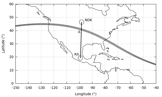
Figure 1: Map of the path of the August 21, 2017 eclipse. The continuous line represent the center of the totality, whereas the lower and upper limits are marked with dashed lines. The great circle from the transmitter (NDK) to the receiver (RX) in Mexico City, Mexico is marked with the thick full line. The point A on the map represents the location of the maximum of the eclipse on our propagation path, the maximum phase of the eclipse at point A occurred at 18:00 UT.

4 VLF Observations

In Figure 2 we show the phase (a) and the amplitude (b) variation of the VLF signals propagating along NDK-RX path, from 10:00 UT on August 21, 2017 to 10:00 UT next day, for the N-S antenna. We marked sunrise (SR) and sunset (SS) according to the diurnal pattern where the phase increases/decreases abruptly, at $\sim$ 12:00 UT and $\sim$ 01:30 UT the next day, respectively. The night-time value of phase is $\sim 0^{\circ}$, while the unperturbed daytime value is $\sim 260^{\circ}$. The amplitude shows similar patterns of sunrise/sunset with an unperturbed daytime value of $\sim 8$ dB. The vertical dashed lines indicate the beginning (16:34 UT), the maximum (18:00 UT) and the end (19:26 UT) of the eclipse along our propagation path.

The bottom panel in Figure 2 represents a rough schematic of the diurnal phase change. We are interested in the ratio of the phase change due to the solar eclipse ($\Delta\Phi_{E}$) and the phase change between the night and day during the sunrise ($\Delta\Phi_{SR}$) and sunset ($\Delta\Phi_{SS}$). The maximum phase change during the eclipse accounted for $\sim$25$\%$ of the total diurnal average phase change. Assuming a total diurnal change (at the reference height) of $\sim$ 20-30 km and an upper limit of the daytime D-region of 90 km of altitude, the eclipse phase change represents a rise in the effective reflection height of the ionosphere of $\sim$ 5-8 km. In Table 1 we present the measured phase change, the ratios of eclipse with respect to day-night phase change and the estimated change in the effective reflection height of the ionosphere.

In panels (c) and (d) of Figure 2, we present a detailed view of the phase and the amplitude changes during the time of the solar eclipse (16:00 - 20:00 UT). For the sake of simplicity, we shifted to zero the values of the phase and the amplitude during unperturbed times. The phase reaches a minimum of -63.36^∘ at 18:05 UT. We note that at the time of the eclipse a C3.0 solar flare occurred, with a maximum at 17:57 UT (in X-ray flux). The flare was powerful enough to shift the phase towards positive values thus distorting the eclipse pattern. In this way, the real minimum should be occurred a few minutes prior to the measured one, at 18:00 UT, which is the time of totality on our propagation path (point A in Figure 1). The change in amplitude reaches a minimum of -4.90 dB at 17:47 UT, however the effect of the C3.0 flare on amplitude is more profound than the case of the phase.

Differences between amplitude and phase time-behavior are regularly seen at sunrise and sunset (Wait, 1968; Muraoka, 1983; Davies, 1965) as clearly seen at 11:30 UT (sunrise) and at 03:30 UT (sunset) in panels (a) and (b) of Figure 2. These are due to the different response of the phase delay and amplitude to the modal conversions due to the sudden changes of the height and surface characteristics of the waveguide (Wait, 1968). Similar differences are seen during the eclipse (panels (c) and (d) of Figure 2). The phase delay is more sensitive than the amplitude to the small changes of the Sun illumination before the second contact. As the quiescent D-layer uplifts at the beginning of the eclipse, the phase velocity of the first-order mode decreases and so does the phase shift. The change of the phase-shift slope may occur when the wave-guide reaches an altitude high enough to allow a significant second-order mode propagating along with the first-order mode causing a further reduction of the phase velocity.

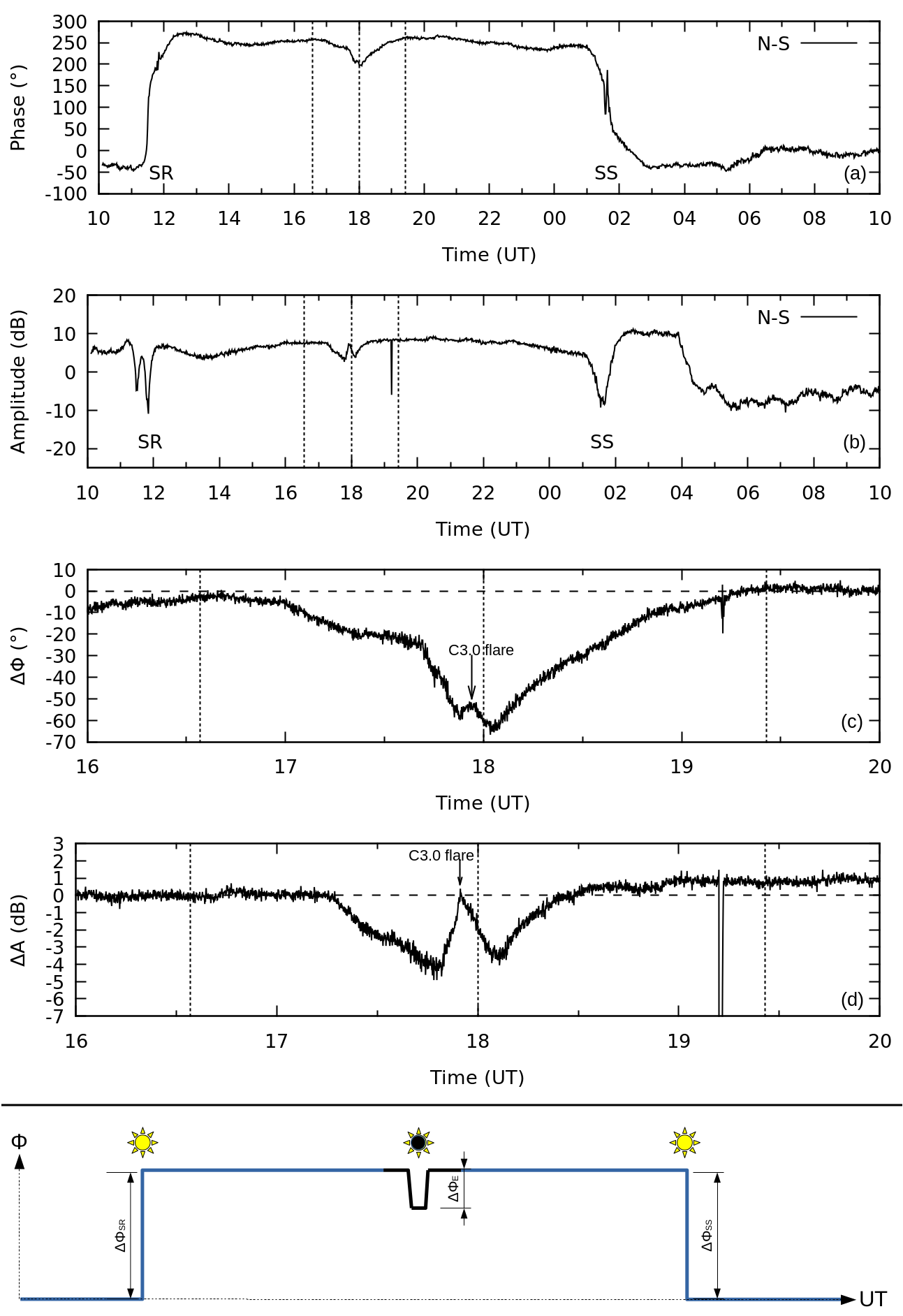
Figure 2: Phase (a) and amplitude (b) variations of the VLF signal along NDK-RX path, from 10:00 UT on August 21, 2017 to 10:00 UT next day, of the N-S antenna. We marked the sunrise (SR) and the sunset (SS) where the phase changes abruptly, according to the diurnal pattern. A detailed view of the phase (c) and the amplitude (d) at the time of the eclipse (16:00 to 20:00 UT). The vertical dashed lines indicate the beginning (16:34 UT), the maximum (18:00 UT) and the end (19:26 UT) of the eclipse along our propagation path. The maximum of the C3.0 solar flare, at 17:57 UT is marked. The bottom panel schematically represents the diurnal phase change. $\Delta\Phi_{E}$ represents a phase change due to the eclipse, while $\Delta\Phi_{SR}$ and $\Delta\Phi_{SS}$ represent a phase change between the night and the day, one at sunrise time (SR) and one at sunset time (SS).

	$\Delta\Phi$(∘)	Ratio	$\Delta$z(km)
Sunrise (SR)	300.15 $\pm$ 4.21	0.24 $\pm$ 0.01	(4.8-7.2) $\pm$ 0.1
Sunset (SS)	273.40 $\pm$ 3.21	0.27 $\pm$ 0.01	(5.4-8.1) $\pm$ 0.1
Eclipse (E)	72.84 $\pm$ 2.60

Table 1: The measured phase (column 2, $\Delta\Phi$) during the sunrise (SR), and sunset (SS); and the corrected value between noon and the eclipse minimum (E). The ratio between phase changes and the expected change of the ionospheric reflection layer $\Delta$z, are in columns 3 and 4.

5 The Eclipse Model

In this section we present a model of the phase deviation during the eclipse. We consider effects such as the equivalent shortening of the propagation path between transmitter and receiver, and increasing of the effective ionospheric reflection height. We start with the equation formulated by Wait (1959), see also Deshpande and Mitra (1972) and Muraoka et al. (1977):

$$\Delta\Phi=360^{\circ}\frac{d}{\lambda}\left(\frac{1}{2a}+\frac{\lambda^{2}}{16z^{3}}\right)\Delta z,$$ (1)

where $\Delta\Phi$ is the phase delay, $d$ is the distance between transmitter and receiver, $\lambda$ is the wavelength of the VLF wave, $a$ is the radius of the Earth, $\Delta z$ is the variation of the reflection height and $z$ is the daytime altitude of the ionosphere. In this analysis we used z = 70.5 km as proposed by Thomson (2010). We note that Equation 1 is valid for a propagation path of distance $d\geq 3000~{}km$ illuminated by the Sun and our propagation path is in the lower limit, even during the eclipse when only a small part of the path is totally obscured by the Moon.

The steps of the eclipse modelling are illustrated in Figure 3. First, in order to filter out the effect of the C3.0 solar flare, we fitted the observed phase profile, at the time of totality (without considering the time of the flare) with a model constructed by the addition of Gaussian curves and due to the asymmetric nature of the phase time profile, the best fit was achieved by adding six Gaussian models (dashed black line in panel a).

Next, we propose that the illuminated propagation path distance is a function of time, since the fraction of the path covered by the eclipse shadow changes rapidly. Thus we can write Equation 1 as:

$$\Delta\Phi(t)=C_{1}\Delta d(t)\Delta z(t),$$ (2)

where $C_{1}=360^{\circ}\frac{1}{\lambda}(\frac{1}{2a}+\frac{\lambda^{2}}{16z^{3}})$ is a constant, $\Delta d(t)$ is a time function of the propagation path distance and $\Delta z(t)$ is a time function of the reflection height variation. We can rewrite Equation 2 in terms of relative changes as:

$$\widetilde{\Phi(t)}=C_{2}\widetilde{d(t)}\Delta z(t),$$ (3)

where the relative phase change is:

$$\widetilde{\Phi(t)}=\frac{\Delta\Phi(t)}{\Phi_{0}}=\frac{\Phi_{0}-\Phi(t)}{\Phi_{0}}=1-\frac{\Phi(t)}{\Phi_{0}};$$ (4)

and the relative propagation path distance is:

$$\widetilde{d(t)}=\frac{d(t)}{d}=\frac{d-\Delta d(t)}{d}=1-\frac{\Delta d(t)}{d};$$ (5)

$C_{2}=C_{1}d/\Phi_{0}$ is a constant where $\Phi_{0}=260.15^{\circ}$ is the daytime value of the phase; $\Phi(t)$ is the measured phase; and $\Delta d(t)$ represents the distance along the propagation path covered by the shadow.

To find out $\widetilde{d(t)}$ we proceed as follows

• Compute, with a time cadence of 1 minute, the altitude and azimuth angles of the Sun and the Moon, as seen by virtual observers located at a set of evenly spaced points (every 10 km) along the propagation path NDK-RX.

• With this, compute the percentage of the solar disk area $A$ covered by the Moon (via a two circle intersection approach, see A for details), seen at each observational point along the propagation path ($d$), as a function of time ($t$), obtaining the curve $A(d,t)$ ($A_{jk}$ in B). Note that, for a fixed time $k$ the function $A(d,t_{k})$ represents the covered area of the solar disk along the entire path (this is equivalent to $A_{k}^{C}$ in B).

• For consistency and to facilitate the computations, in this step, instead $A(d,t_{k})$ we use its percentage (where 100% is the maximum of the solar disk area covered by the moon, observed on the entire time interval and over all observational points, later on we recover the actual value as weighting process in B). Then, compute the distance $\Delta d(t_{k},A_{m})$ (or $\Delta d_{km}$ in B) at a set of evenly spaced percentage values. As an example Figure 3b shows $A(d,t_{k})$ for $t_{k}=$ 18:00 UT with a continuous line and the correspondent $\Delta d(t_{k},A_{m})$ for $m=60\%$ is marked by the horizontal dashed line.

• Substitute $\Delta d(t,A_{m})$ in Equation 5 to obtain $\widetilde{d(t,A_{m})}$, this is the distance illuminated as a function of time and percentage (m). As instance, Figure 3c shows two iso-curves at $m=30\%$ and $80\%$, with long and short dashed lines, respectively; and the colored contours are the same but for different values of m.

• Finally, we define the total change of illuminated distance as the envelope of all the iso-curves. This is shown by the continuous line in Figure 3c (see B for the computational details).

Once we know the effect of the eclipse on the propagation path, we are able to quantify the increase of the effective reflection height of the ionosphere caused by the Moon shadow. In order to find $\Delta z(t)$ (Equation 3), we need to do a discrete convolution over two finite sequences:

$$(f\ast g)[n]=\sum_{m=-M}^{M}f[n-m]g[m],$$ (6)

where $f$ and $g$ are one-dimensional input arrays whose convolution is defined at each overlapping point, in this case $f=1/\widetilde{d(t)}$ and $g=\widetilde{\Phi(t)}$. The resulting convolution (see Figure 3d) is proportional to $C_{2}\Delta z(t)$, which is dimensionless. By normalizing it, we are left with a dimensionless function of reflection height variation $\widetilde{\Delta z(t)}=\Delta z(t)/b$, where $b$ is an unknown parameter in units of km. Putting together equations 3, 4 and 5, we obtain the model of the phase $\Phi_{M}$ as:

$$\Phi_{M}(t)=\Phi_{0}-C_{1}d(t)\widetilde{\Delta z(t)}b.$$ (7)

Still we do not know the value of the parameter $b$. Therefore we compute $\chi^{2}$ between the modelled $\Phi_{M}(t)$ and the measured $\Phi(t)$ for $b\in[0,20]$ km, with a step of 0.1 km. We adopt parameter $b$, where MIN($\chi^{2}$) holds. This directly gives us the profile of the reflection height variation at the time of the eclipse,

$$\Delta z(t)=\widetilde{\Delta z(t)}b.$$ (8)

The best fit between our model and the measured phase is achieved when $b=9.3\pm 0.1$ km, see Figure 3e. Meaning that the estimated rise in reflection height at the time of the maximum eclipse (18:00 UT) on propagation path NDK-RX, is about $\Delta z_{max}=9.3\pm 0.1$ km, see Figure 3f. This means that the effective reflection height of the ionosphere was $z_{max}=80.0\pm 0.5$ km at the time of totality.

As seen in Table 2, the computed $\Delta z$ (marked as this work) is slightly higher than the similar results obtained with the VLF technique, although our result is in very good agreement with the $\Delta z$ computed using rockets.

GCP (km)	$\Delta z$ (km)	Date	Source
1245	8.00	11-Aug-1999	Clilverd et al. (2001)
2820	6.18	30-Jun-1992	Mendes Da Costa et al. (1995)
3007	9.30	21-Aug-2017	This work, Model
3007	5-8	21-Aug-2017	This work, Ratio
4800	3.00	22-Jul-2009	Venkatesham et al. (2019)
5700	3.00	15-Jan-2010	Pal et al. (2012)
5761	3.75	1-Aug-2008	De et al. (2010)
$<10000$	5.14	15-Jan-2010	Guha et al. (2012)
$>10000$	4.85	22-Jul-2009	Guha et al. (2012)
Rocket	8.00	7-Mar-1970	Clilverd et al. (2001)
Rocket	9.00	12-Nov-1966	Clilverd et al. (2001)

Table 2: Change of $\Delta z$ during solar eclipses measured by different authors using VLF waves except for the last two rows, in these cases the measurements were made by rockets. This work model refers to our eclipse model (Secc. 5) and Ratio refers to the basic comparison between the eclipse effect and the Sunrise and Sunset 4.

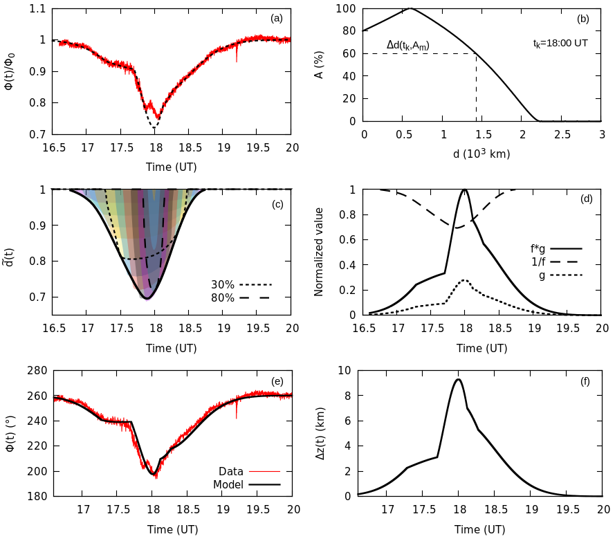
Figure 3: (a) The normalized measured phase $\Phi(t)/\Phi_{0}$ (red) was approximated by the addition of 6-Gaussian profiles (dashed black line). (b) Percentage of the covered solar disk as a function of the distance along the NDK-RX propagation path at 18:00 UT (continuous line) the horizontal dashed line represents the distance where the solar disk was 60% covered at this specific time. (c) The iso-curves of the amount of % covered as a function of time (discontinuous lines to mark 30 and 80% and colored contours mark other percentage levels) and the resulting envelope ($\widetilde{d(t)}$) for the entire time range (thick solid line). (d) The discrete convolution between $f=1/\widetilde{d(t)}$ (dashed line) and $g=\widetilde{\Phi(t)}$, (dot-dashed line). The convolution (continuous line) is proportional to $C_{2}\Delta z(t)$. (e) Our model (black) which best fits the measured phase (red) when $b=9.3\pm 0.1$ km. (f) Change of the ionospheric reflection height during the eclipse.

6 The Flare Input

In this section we investigate the effects of the C3.0 flare occurred at the time of the eclipse, reaching its maximum X-ray flux at 17:57 UT. This event presents a unique opportunity to study the ionospheric conditions during the eclipse, i. e., low background radiation, at the excess flux of a solar flare.

We first take the actual data of phase (NDK-RX) and subtract it from the 6-Gaussian fit, which describes the minimum expected value of the phase at the time of totality over our propagation path. Thus we obtain solely the time profile of the C3.0 flare.

In order to compare the duration and shape of the Solar X-ray flux excess and the associated ionospheric effect observed through the VLF data, we have plotted (see Figure 4) the normalized VLF phase response and the Solar X-ray flux from GOES satellite, 1-8 Å  and 0.5-4.0 Å. We notice a much more sharper profile than the regular response that usually appears in the non-eclipse conditions, i. e., the phase change (due to a Solar flare) behaves in strong accordance with the X-ray flux. This could be attributed to the different (eclipsed) background conditions in the lower ionosphere, causing an increase in the effective recombination coefficient. A detailed study of this event will be published elsewhere.

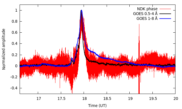
Figure 4: Solar flare X-ray flux from GOES satellite, 0.5-4.0 Å  (black line) and 1-8 Å  (blue line). Vertical axis represents the normalized amplitude of GOES flux and the normalized VLF phase (red) for NDK data.

We use the ionospheric height profile $z=z(t)$, as well as the propagation distance function $d=d(t)$ (see Section 5) and equation 1, but in this case, $\Delta\Phi$ is the phase difference caused by the C3.0 flare; $z(t)=z_{0}+\Delta z_{e}(t)$ corresponds to the ionospheric height profile under the eclipse conditions; and $\Delta z_{e}(t)$ is the eclipsed change of height (after the convolution of Eq. 8, see figure 3f).

We express the flare-induced ionospheric height difference $\Delta z_{f}(t)$ to quantify the flare contribution to the total effective ionospheric height change and then compare the ionospheric height profile during both: the solar eclipse and the solar eclipse combined with the solar flare input, see figure 5. Our results are in good agreement with the same obtained by Chakrabarti et al. (2018), who measured the signal amplitude of 2 receiving stations in North America, YADA in McBaine and KSTD in Tulsa. In the latter they observed similar effects caused by a C3.0 flare. The authors used the LWPC code and the Wait’s two-component D-region ionospheric model, to numerically reproduce the observed signal amplitude variation at both receiving locations. Their altitude profile at maximum electron density for combined effects (solar eclipse and solar flare) correspond well with our results, see Figure 8 in Chakrabarti et al. (2018). This is remarkable due to the relative simplicity of our approach.

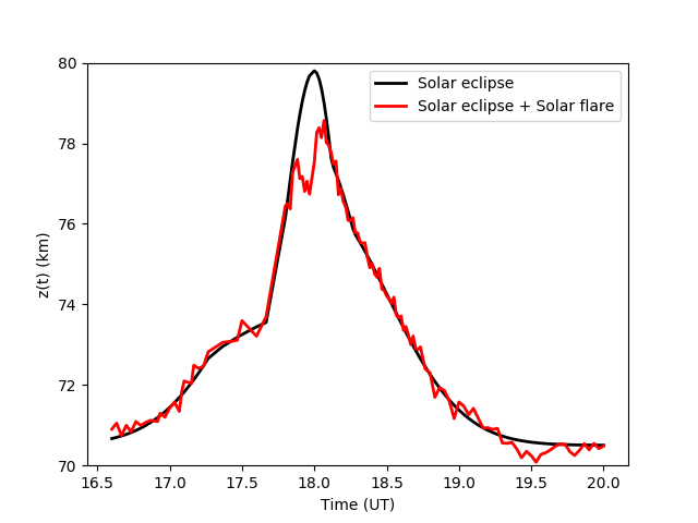
Figure 5: Comparison of ionospheric height of both only the solar eclipse and the solar eclipse combined with the solar flare input. The solar flare contributes to a maximum change of height by about -3 km $\pm$ 1 km.

7 Summary and discussion

We have used the Latin American Very Low Frequency Network at Mexico (LAVNet-Mex) station to study the effects of the August 21, 2017 total solar eclipse on the D-region of the Earth’s ionosphere. Our main goal was to estimate the rise of the reflection height at the time of the eclipse via the measured phase deviation of the received signal from NDK transmitter in ND, USA (at a fixed frequency of 25.2 kHz). We presented the experimental setup used for phase and amplitude measurements of the received VLF waves. Also, we described the so called “Great American Solar Eclipse” and its path across the mainland which crossed almost perpendicularly, the 3007.15 km long propagation path NDK-RX. As expected, the effect of the eclipse caused a decrease in both the phase and the amplitude of the VLF signal.

During the eclipse, a substantial part of the ionosphere above our propagation path received less ionizing radiation from the Sun. Therefore, to estimate the rise of the VLF reflection height, we first approach the problem in a very simple way by using as reference the total night/day change (i. e. at the sunrise and the sunset) of 20-30 km, and calculating the ratio between the maximum eclipse phase change and the day-night phase change. This accounted for $\sim 25\%$ of the total diurnal average phase change, equivalent to a rise in reflection height of about 5-8 km.

Around the totality time (17:57 UT) a C3.0 solar flare occurred and was powerful enough to shift the phase and amplitude to more positive values, distorting the eclipse pattern. To remove its effects, we created a model by adding Gaussian functions to better describe the phase profile during the time of the eclipse totality.

In Section 5 we described our model which considers the eclipse geometry to obtain the area of the solar disk occulted by the Moon as a function of time. At each time is considered the percentage of the GCP darkening and obtained the expected values for phase and height variations of D-region using the Wait (1959), Deshpande and Mitra (1972) and Muraoka et al. (1977) formulations for VLF signal propagation in the Earth-ionosphere waveguide. In particular, we found that at the time of the eclipse totality (18:00 UT), the rise in reflection height was $\Delta z_{max}=9.3\pm 0.1$ km. Therefore, the effective reflection height of the ionosphere rose to approximately $z_{max}=80.0\pm 0.5$ km at the time of totality.

It is important to note that our results of reflection height variation during the eclipse, obtained by two different methods (calculating ratios and eclipse modeling) show a good agreement with the results from similar measurements (Table 2). Particularly, the analysis of the ratio between the ionospheric changes during the eclipse and the day/night transition (Secc. 4) is in very good agreement with the results obtained with similar GCP and analysis method (rows 2 and 4 of Table 2). Whereas the result of the eclipse model (Secc. 5) is slightly higher compared with other similar VLF observations, although it is in very good agreement with the rocket observations (rows 3, 10 and 11 of Table 2). These differences are expected due to the fact that the amount of the reflection height variation during an eclipse depends on the GCP length, and the relative direction of the GCP and the path of the eclipse totality (Venkatesham et al., 2019). In our case, GCP distance was 3007.15 km and it crossed the path of the total eclipse almost perpendicularly.

Finally, our model of the C3 X-ray flare observed during the eclipse is in very good accordance with the results obtained through LWPC simulations reported in Chakrabarti et al. (2018), for a short-length propagation path. This gives support to the use of this model to study of the eclipsed ionosphere.

References

Appendix A The Covered Solar Disk

We present a detailed description of the computation of the covered solar disk area $A(d,t)$. We use the equations of spherical trigonometry to calculate the coordinates of the points ($\Phi_{j},\lambda_{j}$), where j = 1, 2, …, J, were placed every 10 km along the propagation path NDK-RX. Each point is at some distance $d_{j}$ from the origin, which is set at the receiver station in Mexico City. Therefore $d_{1}=0$ and $d_{J}=d$, where $d$ is the propagation path length. The geographic coordinates of the receiver and the transmitter at mutual separation $d$ are known. Then:

$$y=\sin(\lambda_{\mathrm{RX}}-\lambda_{\mathrm{TX}})\cos(\phi_{\mathrm{RX}}),$$ (9)

where $\lambda$ is the geographic longitude, $\phi$ is the geographic latitude, $RX$ denotes receiver and $TX$ denotes transmitter, in our case NDK. Similarly it follows

$$x=\cos(\phi_{\mathrm{TX}})\sin(\phi_{\mathrm{RX}})-\sin(\phi_{\mathrm{TX}})\cos(\phi_{\mathrm{RX}})\cos(\lambda_{\mathrm{RX}}-\lambda_{\mathrm{TX}}).$$ (10)

We need $y$ and $x$ in order to calculate the Bearing angle $\Theta$,

$$\Theta=\mathrm{atan2}(y,x),$$ (11)

where atan2 is an inverse trigonometric function of two arguments, which returns a value between $-\pi$ and $\pi$. We calculate the geographic longitude and latitude of the points along the propagation path of length $d$

$$\phi_{j}=\arcsin\Bigg{(}\sin(\phi_{\mathrm{TX}})\cos{\Bigg{(}\frac{d_{j}}{a}\Bigg{)}}+\cos(\phi_{\mathrm{TX}})\sin\Bigg{(}\frac{d_{j}}{a}\Bigg{)}\cos(\Theta)\Bigg{)},$$ (12)

where $a$ is the radius of the Earth (6370.0 km). Similarly it follows for the geographic latitude

$$\lambda_{j}=\lambda_{\mathrm{TX}}+\mathrm{atan2}\Bigg{(}\sin(\Theta)\sin\Bigg{(}\frac{d_{j}}{a}\Bigg{)}\cos(\phi_{\mathrm{TX}}),\cos\Bigg{(}\frac{d_{j}}{a}\Bigg{)}-\sin(\phi_{\mathrm{TX}})\sin(\phi_{\mathrm{RX}})\Bigg{)}.$$ (13)

The length of the propagation path follows as

$$d=\arccos\Bigg{(}\sin(\phi_{\mathrm{TX}})\sin(\phi_{\mathrm{RX}})+\cos(\phi_{\mathrm{TX}})\cos(\phi_{\mathrm{RX}})\cos(\lambda_{\mathrm{RX}}-\lambda_{\mathrm{TX}})\Bigg{)}a.$$ (14)

We are ready to calculate azimuth and altitude of the Sun and the Moon at every point ($\Phi_{j}$,$\lambda_{j}$) along the propagation path, for all $t_{k}$ (every minute of the eclipse, 16:00 UT – 20:00 UT), where j = 1, 2, …, J and k = 1, 2, …, K. Using astropy.coordinates library that possess reliable ephemeris solar$\_$system$\_$ephemeris.set(^′jpl^′), the coordinates of the Sun and the Moon at an arbitrary time are obtained. Thus we can calculate the angular distance between the centers of the Sun and the Moon as

$$s=\sqrt{(\alpha_{M}-\alpha_{\odot})^{2}+(h_{M}-h_{\odot})^{2}},$$ (15)

where $\alpha$ is azimuth, $h$ is altitude, $M$ denotes the Moon, $\odot$ denotes the Sun. At the time of the eclipse, based from the Earth-ground, radius of the Moon measured $r_{M}$ = 16.06 arcmin and radius of the Sun measured $r_{\odot}$ = 15.81 arcmin. With known angular separation and radii we calculate the area $A’$ of the solar disk that is covered by the Moon using the circle-circle intersection equation

$$A^{\prime}=r_{M}^{2}\arccos\left(\frac{s^{2}+r_{M}^{2}-r_{\odot}^{2}}{2sr_{M}}\right)+r_{\odot}^{2}\arccos\left(\frac{s^{2}-r_{M}^{2}+r_{\odot}^{2}}{2sr_{\odot}}\right)-\\ \frac{1}{2}\sqrt{(-s+r_{M}+r_{\odot})(s+r_{M}-r_{\odot})(s-r_{M}+r_{\odot})(s+r_{M}+r_{\odot})},$$ (16)

where $A^{\prime}$ has a dimension of (arc min)². We are interested in the percentage of the covered Sun, thus it follows

$$A=\Bigg{(}\frac{A^{\prime}}{\pi r_{\odot}^{2}}\Bigg{)}100\%.$$ (17)

We calculate $A$ for every $d_{j}$ along the propagation path of length $d$ and for every $t_{k}$ (step of 1 min) in order to obtain a set of curves $A(d,t)$.

Appendix B Matrix Method

The detailed procedure to model the solar illumination during the eclipse based in a matrix method is as follows:

• Let there be J number of points (every 10 km) along the propagation path of a distance d; we denote each point as $d_{j}$ where j = 1, 2, …, J.

• Let there be K number of time points from start to end (16:00 - 20:00) of the eclipse. Each point is at some distance $d_{j}$ from the origin, which was set at the receiver station in Mexico City. Therefore, $d_{1}=0$ and $d_{J}=d$, where $d$ is the total length of the propagation path (in similar way as in A).

• Let $A(d_{j},t_{k})$ be the calculated area of the covered Sun at an arbitrary point along the propagation path and at an arbitrary time during the eclipse. We first obtain a matrix A of J $\times$ K elements in this way

  $$A=\begin{bmatrix}A_{11}&A_{12}&A_{13}&\dots&A_{1K}\\ A_{21}&A_{22}&A_{23}&\dots&A_{2K}\\ \vdots&\vdots&\vdots&\vdots&\vdots\\ A_{J1}&A_{J2}&A_{J3}&\dots&A_{JK}\end{bmatrix},$$

  where we simplified $A(d_{j},t_{k})$ as $A_{jk}$.

• We now extract each column in the matrix A. Thus we obtain K number of columns of this form

  $$A_{k}^{C}=\begin{bmatrix}A_{1k}\\ A_{2k}\\ \vdots\\ A_{Jk}\end{bmatrix}$$

  where k = 1, 2, …, K and C denotes column. Each $A_{k}^{C}$ can be presented in a graph $A(d,t_{k})$ (see Figure 3b).

• Let there be M number of possible calculated areas of the covered Sun $A$ expressed in $\%$, in our case from 1-99$\%$. We calculate the width of each $A(d,t_{k})$ curve for each m (see Figure 3b), where m = 1, 2, …, M; this gives us $\Delta d(t_{k},A_{m})$ which can be expressed as a K $\times$ M matrix

  $$\Delta d=\begin{bmatrix}\Delta d_{11}&\Delta d_{12}&\Delta d_{13}&\dots&\Delta d_{1M}\\ \Delta d_{21}&\Delta d_{22}&\Delta d_{23}&\dots&\Delta d_{2M}\\ \vdots&\vdots&\vdots&\vdots&\vdots\\ \Delta d_{K1}&\Delta d_{K2}&\Delta d_{K3}&\dots&\Delta d_{KM}\end{bmatrix}.$$

  Similarly we simplified $\Delta d(t_{k},A_{m})$ as $\Delta d_{km}$.

• We now extract each column in the matrix $\Delta d$. Thus we obtain M number of columns of this form

  $$\Delta d_{m}^{C}=\begin{bmatrix}\Delta d_{1m}\\ \Delta d_{2m}\\ \vdots\\ \Delta d_{Km}\end{bmatrix}$$

  where m = 1, 2, …, M and C denotes column. Each $\Delta d_{m}^{C}$ can be presented in a form $\Delta d(t,A_{m})$, which we put into Equation 5 to obtain $\widetilde{d(t,A_{m})}$, where m = 1, 2, …, M.

• Finally we put weights to each of the M functions $\widetilde{d(t,A_{m})}$ in this manner $\widetilde{d(t,A_{m})}\rightarrow A_{m}\widetilde{d(t,A_{m})}$, see dashed lines in Figure 3c. When plotting all weighted $\widetilde{d(t,A_{m})}$ together and taking the envelope around the total effective area under these curves, we finally obtain $\widetilde{d(t)}$ (full thick line in Figure 3c).

References

- Borgazzi et al. (2014) Borgazzi, A., Lara, A., Paz, G., Raulin, J. P., Aug. 2014. The ionosphere and the Latin America VLF Network Mexico (LAVNet-Mex) station. Advances in Space Research 54, 536–545.
- Chakrabarti et al. (2018) Chakrabarti, S. K., Sasmal, S., Chakraborty, S., Basak, T., Tucker, R. L., Aug. 2018. Modeling D-region ionospheric response of the Great American TSE of August 21, 2017 from VLF signal perturbation. Advances in Space Research 62, 651–661.
- Clilverd et al. (2001) Clilverd, M. A., Rodger, C. J., Thomson, N. R., Lichtenberger, J., Steinbach, P., Cannon, P., Angling, M. J., 2001. Total solar eclipse effects on VLF signals: Observations and modeling. Radio Science 36, 773–788.
- Davies (1965) Davies, K., 1965. Ionospheric Radio Propagation. U.S. Dept. of Commerce, National Bureau of Standards, Monograph 80.
- De and Sarkar (1997) De, B. K., Sarkar, S. K., 1997. Anomalous behaviour of 22.3 kHz NWC signal during total solar eclipse of October 24, 1995. Kodaikanal Observatory Bulletins 13, 205–208.
- De et al. (2010) De, S. S., De, B. K., Bandyopadhyay, B., Sarkar, B. K., Paul, S., Haldar, D. K., Barui, S., Datta, A., Paul, S. S., Paul, N., Oct. 2010. The Effects of Solar Eclipse of August 1, 2008 on Earth’s Atmospheric Parameters. Pure and Applied Geophysics 167, 1273–1279.
- Deshpande and Mitra (1972) Deshpande, S. D., Mitra, A. P., Feb 1972. Ionospheric effects of solar flares - IV. Electron density profiles deduced from measurements of SCNA’s and VLF phase and amplitude. Journal of Atmospheric and Terrestrial Physics 34, 255–266.
- Guha et al. (2012) Guha, A., De, B. K., Choudhury, A., Roy, R., Apr. 2012. Spectral character of VLF sferics propagating inside the Earth-ionosphere waveguide during two recent solar eclipses. Journal of Geophysical Research (Space Physics) 117, A04305.
- Kaufmann and Schaal (1968) Kaufmann, P., Schaal, R. E., Mar. 1968. The effect of a total solar eclipse on long path VLF transmission. Journal of Atmospheric and Terrestrial Physics 30, 469–471.
- Mendes Da Costa et al. (1995) Mendes Da Costa, A., Paes Leme, N. M., Rizzo Piazza, L., Jan. 1995. Lower ionosphere effect observed during the 30 june 1992 total solar eclipse. Journal of Atmospheric and Terrestrial Physics 57, 13–17.
- Muraoka (1983) Muraoka, Y., Jan 1983. A new approach to mode conversion effects observed in a mid-latitude VLF transmission. Zeitschrift Angewandte Mathematik und Mechanik 44 (10), 855–862.
- Muraoka et al. (1977) Muraoka, Y., Murata, H., Sato, T., Jul. 1977. The quantitative relationship between VLF phase deviations and 1-8 A solar X-ray fluxes during solar flares. Journal of Atmospheric and Terrestrial Physics 39, 787–792.
- Nicolet and Aikin (1960) Nicolet, M., Aikin, A. C., 1960. The formation of the d region of the ionosphere. Journal of Geophysical Research (1896-1977) 65 (5), 1469–1483.
- Pal et al. (2012) Pal, S., Maji, S. K., Chakrabarti, S. K., Dec 2012. First ever VLF monitoring of the lunar occultation of a solar flare during the 2010 annular solar eclipse and its effects on the D-region electron density profile. Planetary and Space Science, 73 (1), 310–317.
- Raulin et al. (2010) Raulin, J.-P., Bertoni, F. C. P., Gavilán, H. R., Guevara-Day, W., Rodriguez, R., Fernandez, G., Correia, E., Kaufmann, P., Pacini, A., Stekel, T. R. C., Lima, W. L. C., Schuch, N. J., Fagundes, P. R., Hadano, R., Jul. 2010. Solar flare detection sensitivity using the South America VLF Network (SAVNET). Journal of Geophysical Research (Space Physics) 115, A07301.
- Tereshchenko et al. (2015) Tereshchenko, E. D., Sidorenko, A. E., Tereshchenko, P. E., Grigoriev, V. F., Sep. 2015. Effect of the total solar eclipse of 20 March 2015 on the ELF propagation over high-latitude paths. Geophysical Research Letters 42, 6899–6905.
- Thomson (2010) Thomson, N. R., Sep. 2010. Daytime tropical D region parameters from short path VLF phase and amplitude. Journal of Geophysical Research (Space Physics) 115, A09313.
- Venkatesham et al. (2019) Venkatesham, K., Singh, R., Maurya, A. K., Dube, A., Kumar, S., Phanikumar, D. V., Jan 2019. The 22 July 2009 Total Solar Eclipse: Modeling D Region Ionosphere Using Narrowband VLF Observations. Journal of Geophysical Research (Space Physics) 124 (1), 616–627.
- Wait (1959) Wait, J., Dec 1959. Guiding of electromagnetic waves by uniformly rough surfaces : Part I. IEEE Transactions on Antennas and Propagation 7 (5), 154–162.
-
Wait (1968)
Wait, J. R., 6 1968. Mode conversion and refraction effects in the
Earth‐ionosphere waveguide for VLF radio waves. Journal of Geophysical
Research 73 (11), 3537–3548.
URL https://doi.org/10.1029/JA073i011p03537