Collective optimization for variational quantum eigensolvers

Abstract

Variational quantum eigensolver (VQE) optimizes parameterized eigenstates of a Hamiltonian on a quantum processor by updating parameters with a classical computer. Such a hybrid quantum-classical optimization serves as a practical way to leverage up classical algorithms to exploit the power of near-term quantum computing. Here, we develop a hybrid algorithm for VQE, emphasizing the classical side, that can solve a group of related Hamiltonians simultaneously. The algorithm incorporates a snake algorithm into many VQE tasks to collectively optimize variational parameters of different Hamiltonians. Such so-called collective VQEs (cVQEs) is applied for solving molecules with varied bond length, which is a standard problem in quantum chemistry. Numeral simulations show that cVQE is not only more efficient in convergence, but also trends to avoid single VQE task to be trapped in local minimums. The collective optimization utilizes intrinsic relations between related tasks and may inspire advanced hybrid quantum-classical algorithms for solving practical problems.

I Introduction

Quantum computing exploits intrinsic quantum properties for computing. It promises to solve some outstanding problems with quantum advantagesFeynman (1982); Shor (1997); Harrow et al. (2009); Aaronson and Arkhipov (2014); Bravyi et al. (2018); Arute et al. (2019), and is influencing a broad of computational intensive areas, such as quantum simulation Feynman (1982); Abrams and Lloyd (1997); Buluta and Nori (2009); Trabesinger (2012) and machine learning Biamonte et al. (2017). A variational approach for quantum computing sets parameters in a quantum circuit, and learn those parameters through hybrid quantum-classical optimization Yung et al. (2014); Farhi et al. (2014); McClean et al. (2016); O’Malley et al. (2016); Li and Benjamin (2017); McClean et al. (2017a); Shen et al. (2017); Kandala et al. (2017); Hempel et al. (2018); Anschuetz et al. (2018); Mitarai et al. (2018); Moll et al. (2018); Kokail et al. (2019); Takeshita et al. (2019); McArdle et al. (2019); Higgott et al. (2019); Sweke et al. (2019). Such an approach is well suited for near-term quantum processor, and receives lots of attention in recent years Preskill (2018). Among them, variational quantum eigensolver (VQE) aims to solve eigenvalues and eigenstates for quantum systems Yung et al. (2014); McClean et al. (2016); Kandala et al. (2017); Hempel et al. (2018); Liu et al. (2019). The power of representing exponentially large wavefunction on quantum processors and effective hybrid quantum-classical optimization of VQE enhances the ability to solve hard quantum problems.

In many practical problems, a group of related Hamiltonians needs to be solved. For instance, molecule electronic Hamiltonians under different bond lengths or angles, or quantum many-body systems with different interacting strengths. VQE can solve such a group of Hamiltonians one by one independently, without taking advantage of previous results. However, those tasks are mostly similar and related to each other, such that one can exploit intrinsic relations for more efficient optimization that can require less quantum resources or avoid local minimums for single tasks. This is also related to meta learning that draws prior experience for new tasks Andrychowicz et al. (2016); Finn et al. ; Verdon et al. (2019).

In this paper, we propose a hybrid quantum-classical algorithm that can provide a collective optimization for VQE to solve a group of related Hamiltonians simultaneously. It evaluates gradients on the quantum processor and updates variational parameters on the classical computer. Remarkably, the updating process generalizes typically gradient descent into a collective version, which updates variational parameters of different Hamiltonians simultaneously. This is achieved by a snake algorithm Kass et al. (1988); Liu and van Nieuwenburg (2018), originally developed in computer vision Kass et al. (1988), which enforces a smooth condition on variational parameters of different Hamiltonians. We call this collective VQE or cVQE. As demonstrations, we use the cVQE to solve ground-state energies for several molecules at different bond lengths. The advantages of collective optimization are investigated and shown through the flow of variational parameters. Remarkably, the snake algorithm is revealed as a global optimizer, as collective motion of parameters for different tasks can pull a point of parameters for a single Hamiltonian out of traps of local minimums.

The paper is organized as follows. In Sec. II, we review variational quantum eigensolver, and then propose cVQE using the snake algorithm. In Sec. III, we present results of several representative molecules using cVQE. In Sec. IV, we investigate the snake algorithm as a global optimizer. Finally, we give some further discussions and a brief summary.

II Optimization for variational quantum eigensolvers

Solving eigenvalues and eigenstates for a given Hamiltonian is a basic task. Quantum computers provide an avenue for solving eigenstate problems of quantum systems effectively. Different quantum algorithms have been developed for tracking this hard problem, such as quantum phase estimation Aspuru-Guzik et al. (2005), variational quantum eigensolver Yung et al. (2014); McClean et al. (2016), simulating resonance transition of molecules on quantum processors Wang et al. (2012); Li et al. (2019). The VQE approach uses a parameterized quantum circuit to prepare a wavefunction. The parameters are obtained by optimizing the energy with the hybrid quantum-classical algorithm.

To solve quantum systems on a quantum computer, it is necessary to firstly map the original Hamiltonian in a qubit (spin-half) Hamiltonian. For electronic systems, a nonlocal transformation such as Jordan-Wigner transformation Jordan and Wigner (1928) or Bravyi-Kitaev transformation Bravyi and Kitaev (2002), is required to firstly transform fermionic operators into Pauli operators. For a quantum system of interest (e.g., molecules), the resulting qubit Hamiltonian typically has many terms,

$$H=\sum_{i}c_{i}H_{i},$$ (1)

where $H_{i}$ can be written as a tensor product of Pauli matrices, $H_{i}=\otimes_{k}\sigma^{\alpha_{k}}_{k}$. Here $\alpha_{k}=x,y,z$ and $k$ the index of qubits. We now discuss how to solve a single Hamiltonian and a group of related Hamiltonians, respectively.

II.1 Optimization by gradient descent

To find the eigenstate for a single $H$, one can use an ansatz $|\psi(\boldsymbol{\theta})\rangle=U(\boldsymbol{\theta})|\psi_{0}\rangle$ to represent a candidate ground state. Here $|\psi_{0}\rangle$ is an initial state as a good classical approximation as the ground state of $H$. For instance, $|\psi_{0}\rangle$ can be chosen as a Hartee-Fock state in quantum chemistry. $U(\boldsymbol{\theta})$ is an unitary operator parameterized with $\boldsymbol{\theta}$, which can take quantum correlation into consideration. As a variational method, the essential task is to find parameters $\boldsymbol{\theta}_{0}$ that minimizes the energy $\mathcal{E}(\boldsymbol{\theta})=\langle\psi(\boldsymbol{\theta})|H|\psi(\boldsymbol{\theta})\rangle$. The optimization is a hybrid quantum-classical one: the quantum processor runs the quantum circuit and performs measurements to evaluate $\mathcal{E}(\boldsymbol{\theta})$; the classical computer updates parameters $\boldsymbol{\theta}$ according to received data from the quantum processor. To obtain a quantum average of $H$, one can perform measurements for each term $H_{i}$, as it is a tensor product of Pauli matrices thus corresponds to a joint measurement on multi-qubits. Measurements of all terms then are added,

$$\mathcal{E}(\boldsymbol{\theta})=\sum_{i}c_{i}\langle\psi(\boldsymbol{\theta})|H_{i}|\psi(\boldsymbol{\theta})\rangle.$$ (2)

Optimization methods for updating parameters $\boldsymbol{\theta}$ in general can be categorized as gradient free Hempel et al. (2018); Kokail et al. (2019), such as Nelder-Mead method, and gradient descent Kandala et al. (2017); Liu et al. (2019); Sweke et al. (2019). Gradient descent methods update parameters using information of gradients. On a quantum processor, calculating gradient with respect to a target cost function (here is $\mathcal{E}(\boldsymbol{\theta})$) can be obtained with the same quantum circuit, using the shift rule Li et al. (2017); Schuld et al. (2019) or numeral differential. Then parameters $\boldsymbol{\theta}$ are updated with gradient descent as

$$\boldsymbol{\theta}^{t}=\boldsymbol{\theta}^{t-1}-\eta\frac{\partial}{\partial{\boldsymbol{\theta}}}\mathcal{E}(\boldsymbol{\theta}^{t-1}),$$ (3)

where $\eta$ is the learning rate or step size.

II.2 Collective optimization

In the above, variational quantum eigensolver solves the eigenvalue problem for a single Hamiltonian. In practice, there may be a group of Hamiltonians to be solved. For instance, what is needed in quantum chemistry usually is a potential surface, corresponding to ground state energies for a molecule at different bond lengths or bond angles. Of course, one can use VQE to solve Hamiltonians one by one. However, this does not exploit relations between Hamiltonians. Here, we develop a more efficient method that can collectively optimize all variational gate parameters for different Hamiltonians at the same time.

The motivation behind collective optimization can be presented as follows. Consider quantum chemistry problems. Two Hamiltonians should be close to each other if their underlying molecules are the same and bond lengths vary a little. In such a case, the same ansatz can be applied, and it is expected that optimized parameters of wavefunction should be very close to each other. Denoted $\boldsymbol{\theta}_{0}(\lambda)$ as the optimized parameter for Hamiltonian $H(\lambda)$, then $\boldsymbol{\theta}_{0}(\lambda)\sim\lambda$ should form a continuous curve in the space of $\boldsymbol{\theta}$ and $\lambda$, which we call as enlarged parameter space. We expect that the optimization of one Hamiltonian can help optimize other Hamiltonians with nearby system parameters $\lambda$. We use gradient descent for the optimization. Instead of updating a single point in the parameter space, the optimization updates a sequence of points in the enlarged parameter space, each point corresponding to a Hamiltonian. At the continuous limit, this is an optimization of a string.

Now let us elaborate on a concrete algorithm. To incorporate a snake algorithm, the cost function should consider energy of the snake itself, and can be written as follows:

$$L[\boldsymbol{\theta}(\lambda)]=\int_{\lambda_{0}}^{\lambda_{T}}(\mathcal{L}(\boldsymbol{\theta}(\lambda))+\mathcal{E}(\boldsymbol{\theta}(\lambda)))$$ (4)

Here $\mathcal{E}(\boldsymbol{\theta}(\lambda))=\langle\psi(\boldsymbol{\theta}(\lambda))|H_{\lambda}|\psi(\boldsymbol{\theta}(\lambda))\rangle$ is the local potential the snake feels and the internal property is

$$\mathcal{L}(\boldsymbol{\theta}(\lambda))=\alpha|\frac{\partial\boldsymbol{\theta}(\lambda)}{\partial\lambda}|^{2}+\beta|\frac{\partial^{2}\boldsymbol{\theta}(\lambda)}{\partial^{2}\lambda}|^{2},$$ (5)

where $\alpha$ and $\beta$ terms make the snake stretchable and bendable Kass et al. (1988); Liu and van Nieuwenburg (2018), respectively.

Solving the snake can be achieved by minimizing Eq. 4, which can converted to solve a differential equation(see Eq. 7 in the Appendix). For this we discrete the snake as a sequence of parameters at different bond lengths $\mathbf{r}_{i}=(\boldsymbol{\theta}_{i}(\lambda_{1}),\boldsymbol{\theta}_{i}(\lambda_{2}),...,\boldsymbol{\theta}_{i}(\lambda_{M}))$, where $i$ is the $i$-th component for each $\boldsymbol{\theta}_{i}(\lambda_{m})$. Then, the discrete snake can be solved iteratively as

$$\mathbf{r}_{i}^{t}=\left(\eta\boldsymbol{A}+\boldsymbol{I}\right)^{-1}\left(\mathbf{r}_{i}^{t-1}-\eta\frac{dE(\mathbf{r}^{t-1})}{d\mathbf{r}_{i}}\right)$$ (6)

where $E(\mathbf{r})=\sum_{m}\mathcal{E}(\boldsymbol{\theta}_{\lambda_{m}})$, and $\boldsymbol{A}$ is a pentadiagonal banded matrix with nonzero elements depending on $\alpha$ and $\beta$. Details can be found in the Appendix A. Compared with Eq. (3), Eq. (6) can be viewed as a collective gradient descent, as the later is reduced to the former at $\alpha=\beta=0$.

There is an issue for incorporating the snake algorithm into optimizing variational quantum eigensolver. The equilibrium condition Eq. (8) (or Eq. (7)) is actually not the original one $\frac{d\mathcal{E}(\boldsymbol{\theta}(\lambda_{i}))}{d\boldsymbol{\theta}(\lambda_{i})}=0$, as there are interactions between neighbor $\boldsymbol{\theta}(\lambda_{i})$. As a result, optimization with a gradient flow using Eq. (6) may not give the required optimal results. In practice, nevertheless, this issue may be largely ignored, as explained in the following. For neighbor $\lambda_{i}$, it can expected that $\boldsymbol{\theta}(\lambda_{i+1})+\boldsymbol{\theta}(\lambda_{i-1})\approx 2\boldsymbol{\theta}(\lambda_{i}))$ and $\boldsymbol{\theta}(\lambda_{i+2})+\boldsymbol{\theta}(\lambda_{i-2})\approx 2\boldsymbol{\theta}(\lambda_{i}))$ once the optimization is good enough and $M$ is large enough. It can be checked that the first term of Eq. 8 can be approximated as zero, which is consist with the equilibrium condition for VQE, namely by omitting the first term.

In practice, we can introduce a decaying matrix $\boldsymbol{A}(t)=\boldsymbol{A}_{0}\exp(-t\Gamma)$ in the optimization process. For large $t$ limit, this become the gradient descent of Eq. 3. An analog may be made with the annealing methods widely applied for optimization. Internal forces play the role of temperature. Initially, internal forces are large and parameters for different Hamiltonians flow in the space collectively. With decaying internal forces flows of different parameters become more independent. This may inspire us that the snake algorithm may help avoid the optimization to be trapped in a local minimum for a single VQE, which will be investigated at Sec. IV.

III Application of cVQE for molecules

In this section, we apply cVQE for several representative molecules, including molecular hydrogen, Lithium hydride and Helium hydride cation and present their results. The numerical simulations are performed by using Huawei HiQsimulator framework team . It is shown that ground state energies are obtained with great accuracy compared with results using variational quantum eigensolver for Hamiltonian at each bond length alone. Remarkably, variational parameters for ground states of Hamiltonians at different bond lengths collectively flow to optimal values. We present the main results and details of the calculation of Hamiltonians for all molecules at different bond lengths as well as their wavefunction ansatz are put in Appendix. B.

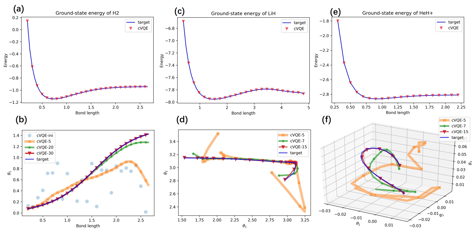
Figure 1: Collective optimization with the snake algorithm for molecules at different bond lengths. The first row shows the target energies and optimization results for the cVQE algorithm, and the second row presents optimization process of variational parameters. The left, the middle and the right columns correspond molecules $\text{H}_{2}$, LiH and $\text{HeH}^{+}$, with one, two, and three variational parameters, respectively.

III.1 Molecular hydrogen

For $\text{H}_{2}$, we consider an effective qubit Hamiltonian involves two qubits, following Ref. Hempel et al. (2018). The unitary coupled cluster (UCC) ansatz is used, with unitary operator

$$U(\theta)=\exp(-i\theta\sigma_{0}^{x}\sigma_{1}^{y})$$

performing on Hartree-Fock reference state is $|01\rangle$. We chose $54$ points uniformly from bond lengths ranging from $0.25$ a.u. to $2.85$ a.u. Effective Hamiltonians corresponding to those bond lengths are obtained with OpenFermion McClean et al. (2017b) Variational parameters are randomly initialized. We set $\alpha=0.1,\beta=3,\eta=0.5$ in the Eq. (6) (note that $\boldsymbol{A}$ depends on $\alpha$ and $\beta$). Ground state energies at different bond lengths fit perfectly with ideal results. Remarkably, variational parameters for different bond lengths, while initialized randomly, quickly form a smooth curve and evolve to the target optimal values, as shown in Fig. (1). This can be understood as a collective optimization process that exploits intricate relations between VQE tasks for Hamiltonians with different bond lengths.

III.2 Lithium hydride

For LiH, STO-6G basis is used to construct the electronic Hamiltonian, which is mapped into a qubit Hamiltonian with BK transformation. Following Ref. Hempel et al. (2018), three orbitals are chosen that the final qubit Hamiltonian evolves three qubits. The UCC operator $U(\theta_{1},\theta_{2})=\exp(-i\theta_{1}\sigma_{0}^{x}\sigma_{1}^{y})\exp(-i\theta_{2}\sigma_{0}^{x}\sigma_{2}^{y})$ performs on an initial state $|111\rangle$. The operator can be taken as two UCCs, and each can be decomposed as in the Eq.(5). Effective Hamiltonians are calculated with OpenFermion from $50$ bond lengths, uniformly chosen from 0.3 a.u. to 5.0 a.u. Variational parameters are randomly initialized. We set $\alpha=0.1,\beta=3,\eta=0.2$ in the Eq. (6). It can be seen in Fig. (1) that potential surface fit well with ideal results. Evolution of variational parameters turns to be rather impressive. Unlike the case of molecular Hydrogen, there are two parameters for each VQE, and thus all points form a curve in the parameter space. The initial curve is random (due to random initialization) and is far away from the target. Nevertheless, the curve flows to the target curve by both shifting and changing its shape. Such a collective optimization process strikingly reminds of the behavior of a crawling snake.

III.3 Helium hydride cation

We now turn to consider Helium hydride cation, which is a more complicated molecular carrying one positive charge. Under STO-3G basis, four qubits are required to describe the Hamiltonian Shen et al. (2017). To capture essential quantum correlation, the UCC ansatz should include a two-particle scattering component Shen et al. (2017). The unitary operator can be written as $U(\theta_{1},\theta_{2},\theta_{3})=\exp(-i\theta_{3}\sigma_{0}^{x}\sigma_{1}^{x}\sigma_{2}^{x}\sigma_{3}^{y})\exp(-i\theta_{2}\sigma_{1}^{x}\sigma_{3}^{y})\exp(-i\theta_{1}\sigma_{0}^{x}\sigma_{2}^{y})$. Effective Hamiltonians are calculated with OpenFermion from $30$ bond lengths, ranging from 0.25 a.u. to 2.5 a.u. Hyper parameters for the snake are set as $\alpha=0.1,\beta=3,\eta=0.2$ in the Eq. (6). As there are three variational parameters, their evolution can be visualized as a crawling snake in a three dimensional space. Although initialized randomly, the snake becomes more smooth and moves to the target position. This again demonstrates the feature of the snake algorithm as a collective optimization process.

IV Nonconvex optimization of cVQE

In the above, we have applied cVQE for solving ground-state energies of several molecules at different bond lengths. The process of optimization shows that parameters for different bond lengths evolve more smoothly, a remarkable feature of the snake algorithm for collective optimization. In this section, we further reveal that the snake algorithm trends for a global optimization, avoiding to be trapped at local minimums.

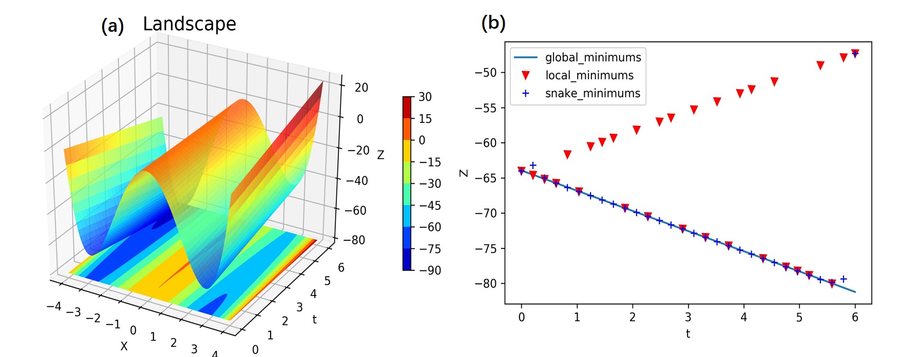
Figure 2: Optimization for a group of Styblinski-Tang functions parameterized with $t$ ($0\leq t\leq 6$). $f(x;t)=\frac{1}{2}(x^{4}-16x^{2}+tx)$. (a). The landscape for a ST function has two minimums for fixed $t$. (b). Optimizations with gradient descent and the snake algorithm. It is shown that local minimums are often achieved by gradient descent why the snake algorithm can mostly achieve global minimums.

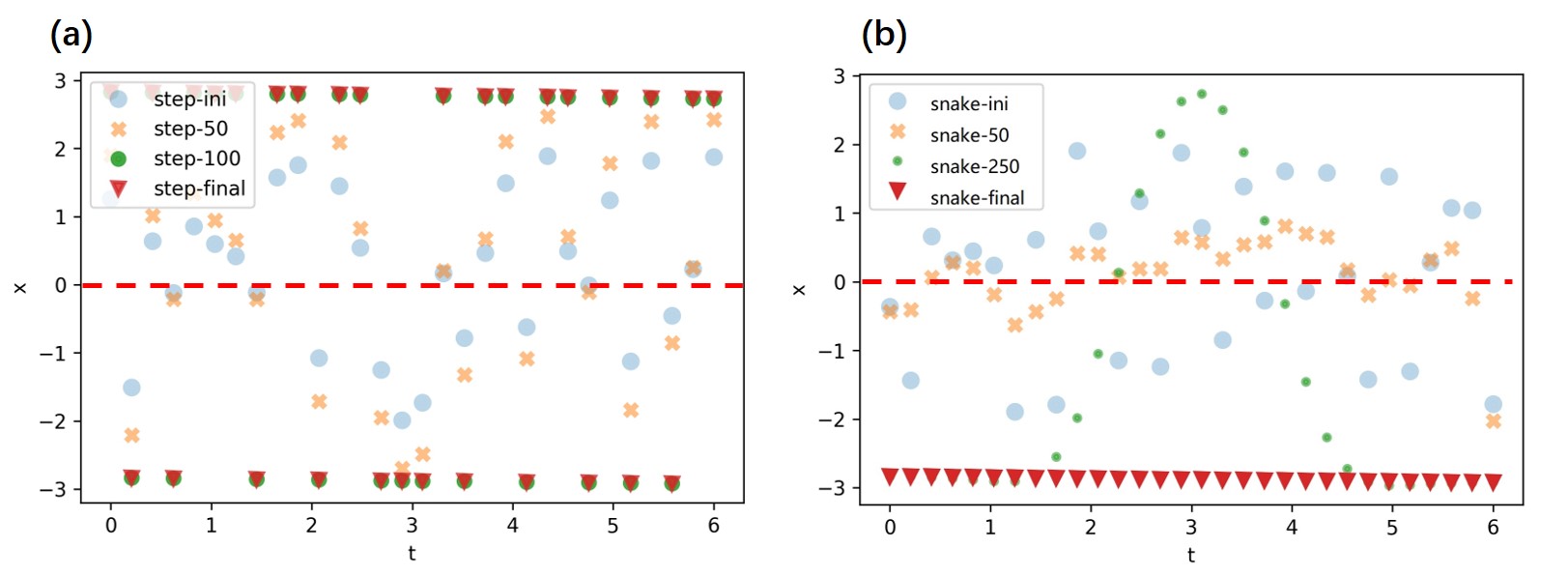
Figure 3: Optimization processes for nonconvex function. (a). Optimization by gradient descent. The flow of $x$ at fixed $t$ depends on the sign of initial value $x_{0}$, and if $x_{0}$ is positive then the optimization goes to the local minimum. (b). Optimization by the snake algorithm. It can be seen that almost all $x$ flow to global minimums collectively, even if they are initialized as positive and negative randomly.

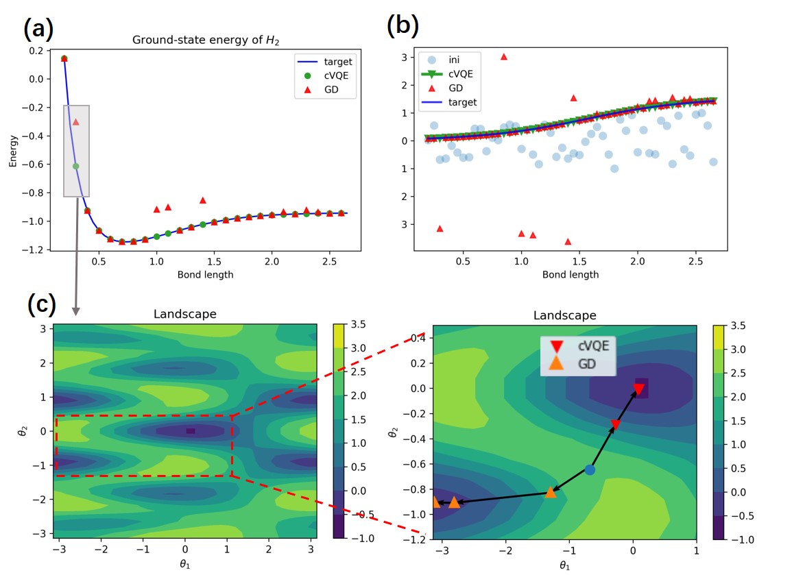
Figure 4: Nonconvex optimization for hydrogen molecule with the cVQE algorithm. (a). Optimization results using both the cVQE algorithm (marked as cVQE) and gradient descent (marked as GD).(b). Evolving of parameters $\theta_{1}$ for the optimization process using the cVQE algorithm (greed line) and gradient descent(red triangular).(c). The landscape for VQE of hydrogen molecule has several different minimums. The random initial point flows to global minimum in cVQE metheod and to a local minimum in gradient descent.

IV.1 Snake algorithm for nonconvex function

We first use a toy example to illustrate how a collective optimization with the snake algorithm can avoid an optimization process to be trapped in local minimums. We consider to minimize the Styblinski-Tang (ST) function Styblinski and Tang (1990), a nonconvex function used to benchmark optimization algorithms, defined as $f(x)=\frac{1}{2}\sum_{i=1}^{N}x_{i}^{4}-16x_{i}^{2}+t_{i}x_{i}$. To illustrate the mechanism of the snake algorithm for nonconvex optimization, we take $N=1$ and consider a group of ST functions, parameterized with $t$ as $f(x;t)=\frac{1}{2}(x^{4}-16x^{2}+tx)$, where $t\geq 0$. For fixed $t$, there are two minimums locating at $\pm x_{0}(t)$ and the global one locates at $-x_{0}(t)$ (assuming $x_{0}(t)>0$). However, those traps are deep that a optimizer may be easily trapped at local minimums, especially for optimizers based on gradient descents. The snake algorithm, although using gradient descent, can avoid this issue. As seen in Fig. (2), most optimal points for different TS functions locate at global minimums. This is because all points are interconnected and can be optimized collectively. Initially, there are some points located at traps of global minimums with random initialization. Then, those points will pull other point out of traps of local minimums, as seen in Fig. (3)b. Such a mechanism can explain why the snake algorithm can be used as an optimizer for nonconvex function.

IV.2 Nonconvex optimization for VQE

For variational quantum eigensolver, an expectation of Hamiltonian with regard to the variational wavefunction ansatz is in general a nonconvex function of variational parameters. As for illustration, we still consider the hydrogen molecule with the same Hamiltonian as Eq.(10), but the wavefunction ansatz is changed to

$$U(\theta_{1},\theta_{2})=\exp(-i\theta_{2}(a\sigma_{0}^{x}+b\sigma_{1}^{x}))\exp(-i\theta_{1}\sigma_{0}^{x}\sigma_{1}^{y}).$$

Here $a$ and $b$ are fixed and we set $a=2,b=1.5$ for instance. Compared to the origin unitary coupled cluster ansatz, there is an extra term $\exp(-i\theta_{2}(a\sigma_{0}^{x}+b\sigma_{1}^{x}))$. As seen in Fig. (4)b, the landscape has several different minimums. The global one locates at the center, corresponding to $\theta_{2}=0$. This is expected as the case of $\theta_{2}=0$ the wavefunction respects particle conservation, which is required for the system of hydrogen molecule. A simple gradient descent as Eq. (3) may lead to local minimums, once initially parameters of $(\theta_{1},\theta_{2})$ are in traps of local minimums (Fig. (4)a). In fact, $\theta_{2}$ corresponding to those local minimums are far from zero, as seen in Fig. (4)c. However, the snake algorithm can perfectly overcome the issue of local minimums for optimizing VQE. During the optimization process, $\theta_{1}$ at different bond lengths evolve collectively. The curve connecting different $\theta_{2}$ becomes more smooth when approaching the target. Meanwhile, and all $\theta_{1}$ shrink to zero. Those present nice feature for nonconvex optimizations that are often met in VQE for quantum chemistry problems.

V Discussion and summary

Optimization is a key component for variational quantum eigensolvers. Here we have incorporated the snake algorithm for optimization of a group of VQE to find ground state energies for a molecular at different bond lengths. As the first step for collective optimization for quantum chemistry/many-body problems, it is expected that cVQE can be tested on more general wavefunction ansatzes. We have applied the unitary coupled cluster ansatz for quantum chemistry problem, and only consider a small number of variational parameters. For many quantum chemistry/many-body problems, more variational parameters are required and also other wavefunction ansatzes may be more suitable Liu et al. (2019). The snake algorithm can be studied for such high dimensional optimization problem. It is expected that the snake algorithm can help to escape local minimums that often appear in a high-dimensional landscape.

In summary, we have incorporated the snake algorithm to optimize variational quantum eigensolvers for a group of Hamiltonians. The cVQE has been used to solve ground states of molecules at different bond lengths simultaneously, which is enhanced by the collective optimization. Remarkably, we have demonstrated that the snake algorithm is a global optimizer, as the collective motion of variational parameters for different tasks can help pull parameters out of traps of local minimums.

Appendix A Collective gradient descent

In this section, we give details of deriving Eq. (6). The snake is determined from the least action principal. This is achieved by minimizing $L[\boldsymbol{\theta}(\lambda)]$. By Euler-Lagrange equation, this leads to a fourth-order differential equation,

$$\alpha\frac{\partial^{2}\boldsymbol{\theta}(\lambda)}{\partial^{2}\lambda}+\beta\frac{\partial^{4}\boldsymbol{\theta}(\lambda)}{\partial^{4}\lambda}+\frac{dE}{d\boldsymbol{\theta}(\lambda)}=0.$$ (7)

Here $E=\int_{\lambda_{0}}^{\lambda_{T}}\mathcal{E}(\boldsymbol{\theta}(\lambda))$. The last term of Eq.(7) should be evaluated on a quantum processor, which makes Eq. (7) rather special and it is expected a solution with a hybrid quantum-classical algorithm.

The Eq. (7) should be solved numerally in a discrete version. $M$ different parameters are chosen uniformly from $[\lambda_{0},\lambda_{T}]$ as $\{\lambda_{1},\lambda_{2},...,\lambda_{M}\}$, and $\lambda_{T}-\lambda_{0}=M\delta$. Using finite difference, the second and forth orders of differentials turns to be Eq. (7),

$$\left[\boldsymbol{\theta}(\lambda_{i+1})-2\boldsymbol{\theta}(\lambda_{i})+\boldsymbol{\theta}(\lambda_{i-1})\right]/{\delta^{2}},$$

$$\left[\boldsymbol{\theta}(\lambda_{i-2})-4\boldsymbol{\theta}(\lambda_{i-1})+6\boldsymbol{\theta}(\lambda_{i})-4\boldsymbol{\theta}(\lambda_{i+1})+\boldsymbol{\theta}(\lambda_{i+2})\right]/{\delta^{4}}$$

respectively. Then we have

$$\boldsymbol{A}\mathbf{r}_{i}+\frac{dE(\mathbf{r})}{d\mathbf{r}_{i}}=0,~{}~{}i=1,2,...,N.$$ (8)

For convenience we also introduce $\mathbf{r}_{i}=(\boldsymbol{\theta}_{i}(\lambda_{1}),\boldsymbol{\theta}_{i}(\lambda_{2}),...,\boldsymbol{\theta}_{i}(\lambda_{M}))$, and denote $E(\mathbf{r})=\sum_{i}\mathcal{E}(\boldsymbol{\theta}_{\lambda_{i}})$. $\boldsymbol{A}$ is a pentadiagonal banded matrix with nonzero elements (under the periodic condition), $\boldsymbol{A}_{i-2,i}=\boldsymbol{A}_{i,i-2}=\beta$, $\boldsymbol{A}_{i-1,i}=\boldsymbol{A}_{i,i-1}=-\alpha-4\beta$,$\boldsymbol{A}_{i,i}=2\alpha+6\beta$, where $\delta^{2}$ and $\delta^{4}$ are absorbed accordingly.

Following Ref.Kass et al. (1988), the equation Eq. (8) can be solved by introducing gradient flow (with an explicit Euler step, so it uses $\boldsymbol{A}\mathbf{r}_{i}^{t}$ instead of $\boldsymbol{A}\mathbf{r}_{i}^{t-1}$),

$$-\frac{\mathbf{r}_{i}^{t}-\mathbf{r}_{i}^{t-1}}{\eta}=\boldsymbol{A}\mathbf{r}_{i}^{t}+\frac{dE(\mathbf{r}^{t-1})}{d\mathbf{r}_{i}},$$ (9)

which leads to Eq. (6).

Appendix B Hamiltonians and unitary cluster ansatz

Solving eigenvalues of electronic structures of molecules is the central problem for quantum chemistry. The ground-state energy is especially important as it largely determines the chemical properties of molecules. The electronic Hamiltonian for a molecule consists of nuclear charges and electrons with Coulomb interactions. By Born-Oppenheimer approximation locations of nuclear are fixed. The electronic Hamiltonian is usually reformulated in the second quantized formulation, with a basis of $N$ molecular orbitals that are a linear combination of atomic orbitals. This can reduce the infinite dimension space of the original real space into a finite Hilbert space. Solving eigenvalues and eigenstates can be done in this subspace. The dimensionality $N$ can be adjusted for the sake of precision demanded.

In the second quantization, the Hilbert space still grows exponentially with the number of orbitals $N$. It is important to only consider orbitals that contribute significantly to the low state energy. In practices, only active orbitals are considered, and inactive ones, such as occupied orbitals very close to the nuclear, or outside empty orbitals are ignored. This leads to an effective electronic Hamiltonian that allows for feasible solutions.

The electronic Hamiltonian is fermionic and still can not be solved on a quantum processor. To map fermionic operators into qubit operators, one can refer to Jordan-Wigner transformation or Bravyi-Kitaev transformation. Those transformations are nonlocal and may introduce a tensor product of a string of Pauli matrices in the qubit Hamiltonian.

We consider three kinds of molecules, molecular hydrogen and Lithium hydride, and helium hydride cation. Their qubit Hamiltonians with varying bond lengths are calculated with the open source software OpenFermion McClean et al. (2017b), following setups in Ref.Hempel et al. (2018) for hydrogen and Lithium hydride, and Ref.Shen et al. (2017) for helium hydride cation.

For $\text{H}_{2}$, and STO-3G minimal basis are adopted, the final effective qubit Hamiltonian involves two qubits, which can be written as

$$H_{\text{H}_{2}}(\lambda) = c_{0}(\lambda)\mathcal{I}+c_{1}(\lambda)\sigma_{0}^{z}+c_{2}(\lambda)\sigma_{1}^{z}+c_{3}(\lambda)\sigma_{0}^{z}\sigma_{1}^{z}$$ (10)

$$+ c_{4}(\lambda)\sigma_{0}^{x}\sigma_{1}^{x}+c_{5}(\lambda)\sigma_{0}^{y}\sigma_{1}^{y}.$$

Here, coefficients $c_{i}(\lambda)$ depend on the bond length $\lambda$ and their values can be found in the code. The Hartree-Fock reference state is $|01\rangle$.

For LiH, STO-6G basis is used to construct the electronic Hamiltonian, which is mapped into a qubit Hamiltonian with BK transformation. Following ref.cite, three orbitals are chosen that the final qubit Hamiltonian evolves three qubits,

$$H_{\text{LiH}}(\lambda)$$

$$=c_{0}(\lambda)\mathcal{I}+c_{1}(\lambda)\sigma_{0}^{z}+c_{2}(\lambda)\sigma_{1}^{z}+c_{3}(\lambda)\sigma_{2}^{z}+c_{4}(\lambda)\sigma_{0}^{z}\sigma_{1}^{z}$$

$$+c_{5}(\lambda)\sigma_{0}^{z}\sigma_{2}^{z}+c_{6}(\lambda)\sigma_{1}^{z}\sigma_{2}^{z}+c_{7}(\lambda)\sigma_{0}^{x}\sigma_{1}^{x}+c_{8}(\lambda)\sigma_{0}^{x}\sigma_{2}^{x}$$

$$+c_{9}(\lambda)\sigma_{1}^{x}\sigma_{2}^{x}+c_{1}0(\lambda)\sigma_{0}^{y}\sigma_{1}^{y}+c_{10}(\lambda)\sigma_{0}^{y}\sigma_{2}^{y}+c_{11}(\lambda)\sigma_{1}^{y}\sigma_{2}^{y}$$

The reference state is $|001\rangle$.

For the above two effective qubit Hamiltonians, we adopt simple unitary coupled cluster ansatz Chan et al. (2004); Taube and Bartlett (2006); Yung et al. (2014); Shen et al. (2017); Hempel et al. (2018), which can establish entanglement between different qubits and thus take quantum correlations into account. For $H_{2}$, the unitary operator is

$$U(\theta)=\exp(-i\theta\sigma_{0}^{x}\sigma_{1}^{y})$$

and the wavefunciton ansatz is $U(\theta)|01\rangle$. The parameter $\theta$ can character the degree of entanglement the electron and the hole. For LiH, the UCC ansatz is

$$U(\theta_{1},\theta_{2})=\exp(-i\theta_{2}\sigma_{0}^{x}\sigma_{2}^{y})\exp(-i\theta_{1}\sigma_{0}^{x}\sigma_{1}^{y}),$$

and the wavefunciton ansatz is $U(\theta_{1},\theta_{2})|111\rangle$. $U(\theta_{1},\theta_{2})$ can be decoupled as two entanglers that establish an entanglement of the zeroth and the first orbitals, the zeroth and the second orbitals, respectively. Two parameters $\theta_{1}$ and $\theta_{2}$ characterize the degrees of entanglement, correspondingly.

We also consider helium hydride cation ($\text{HeH}^{+}$). Under STO-3G basis, its qubit Hamiltonian includes both two, three and four spin interactions.

$$H_{\text{HeH}^{+}}(\lambda) = c_{0}I+\sum_{i=0}^{3}c_{i}Z_{i}+\sum_{i,j=0}^{3}(z_{ij}Z_{i}Z_{j}+x_{ij}X_{i}X_{j}+y_{ij}Y_{i}Y_{j})+\sum_{i=0}^{1}t_{3}(X_{i}Z_{i+1}X_{i+2}+Y_{i}Z_{i+1}Y_{i+2})$$

$$+f_{0}X_{0}X_{1}Y_{2}Y_{3}+f_{1}Y_{0}Y_{1}X_{2}X_{3}+f_{2}X_{0}Y_{1}Y_{2}X_{3}+f_{3}Y_{0}X_{1}X_{2}Y_{3}$$

$$+f_{4}X_{0}Z_{1}X_{2}Z_{3}+f_{5}Z_{0}X_{1}Z_{2}X_{3}+f_{6}Y_{0}Z_{1}Y_{2}Z_{3}+f_{7}Z_{0}Y_{1}Z_{2}Y_{3}.$$

An UCC ansatz for $H_{\text{HeH}^{+}}(\lambda)$ should consider both first and second excitation. Following ref. Shen et al. (2017), we use

$$U(\theta_{1},\theta_{2},\theta_{3})=$$

$$\exp(-i\theta_{3}\sigma_{0}^{x}\sigma_{1}^{x}\sigma_{2}^{x}\sigma_{3}^{y})\exp(-i\theta_{2}\sigma_{1}^{x}\sigma_{3}^{y})\exp(-i\theta_{1}\sigma_{0}^{x}\sigma_{2}^{y}).$$

The wavefunciton ansatz is $U(\theta_{1},\theta_{2},\theta_{3})|0011\rangle$.

To implement the above ansatzes on quantum processors, we need to decompose Hamiltonian evolution of one-particle transition and two-particle transition into a set of universal quantum gates involving single-qubit rotations and two-qubit CNOT gate, as can be seen in Fig (5)

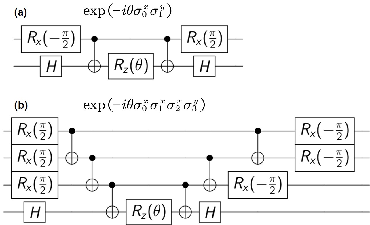
Figure 5: Decomposition of basic operator in unitary coupled cluster ansatz into a set of universal quantum gates.

The decomposition makes the UCC operator implementable on quantum chips. Moreover, variational parameters only appear in a single-qubit rotation $R_{z}(\theta)$. Thus, an analytic gradient can be evaluated using the shift rule.

References

- Feynman (1982) Richard P. Feynman, “Simulating physics with computers,” Int. J. Theor. Phys. 21, 467–488 (1982).
- Shor (1997) Peter W. Shor, “Polynomial-time algorithms for prime factorization and discrete logarithms on a quantum computer,” Siam. J. Comput. 26, 1484–1509 (1997).
- Harrow et al. (2009) A. W. Harrow, A. Hassidim, and S. Lloyd, “Quantum algorithm for linear systems of equations,” Phys. Rev. Lett. 103, 150502 (2009).
- Aaronson and Arkhipov (2014) Scott Aaronson and Alex Arkhipov, “The computational complexity of linear optics,” in Research in Optical Sciences, OSA Technical Digest (online) (Optical Society of America, 2014) p. QTh1A.2.
- Bravyi et al. (2018) Sergey Bravyi, David Gosset, and Robert König, “Quantum advantage with shallow circuits,” Science 362, 308–311 (2018).
- Arute et al. (2019) Frank Arute, Kunal Arya, Ryan Babbush, Dave Bacon, Joseph C. Bardin, Rami Barends, Rupak Biswas, Sergio Boixo, Fernando G. S. L. Brandao, et al., “Quantum supremacy using a programmable superconducting processor,” Nature 574 (2019), 10.1038/s41586-019-1666-5.
- Abrams and Lloyd (1997) Daniel S. Abrams and Seth Lloyd, “Simulation of many-body fermi systems on a universal quantum computer,” Phys. Rev. Lett. 79, 2586–2589 (1997).
- Buluta and Nori (2009) Iulia Buluta and Franco Nori, “Quantum simulators,” Science 326, 108–111 (2009).
- Trabesinger (2012) Andreas Trabesinger, “Quantum simulation,” Nat. Phys. 8, 263 (2012).
- Biamonte et al. (2017) J. Biamonte, P. Wittek, N. Pancotti, P. Rebentrost, N. Wiebe, and S. Lloyd, “Quantum machine learning,” Nature 549, 195–202 (2017).
- Yung et al. (2014) M. H. Yung, J. Casanova, A. Mezzacapo, J. McClean, L. Lamata, A. Aspuru-Guzik, and E. Solano, “From transistor to trapped-ion computers for quantum chemistry,” Scientific Reports 4, 3589 (2014).
- Farhi et al. (2014) Edward Farhi, Jeffrey Goldstone, and Sam Gutmann, “A quantum approximate optimization algorithm,” arXiv:1411.4028 (2014).
- McClean et al. (2016) Jarrod R. McClean, Jonathan Romero, Ryan Babbush, and Alán Aspuru-Guzik, “The theory of variational hybrid quantum-classical algorithms,” New Journal of Physics 18, 023023 (2016).
- O’Malley et al. (2016) P. J J O’Malley, R. Babbush, I. D Kivlichan, J. Romero, J. R McClean, R. Barends, J. Kelly, P. Roushan, A. Tranter, N. Ding, et al., “Scalable quantum simulation of molecular energies,” Physical Review X 6, 031007 (2016).
- Li and Benjamin (2017) Ying Li and Simon C. Benjamin, “Efficient variational quantum simulator incorporating active error minimization,” Physical Review X 7, 021050 (2017).
- McClean et al. (2017a) Jarrod R. McClean, Mollie E. Kimchi-Schwartz, Jonathan Carter, and Wibe A. de Jong, “Hybrid quantum-classical hierarchy for mitigation of decoherence and determination of excited states,” Phys. Rev. A 95, 042308 (2017a).
- Shen et al. (2017) Yangchao Shen, Xiang Zhang, Shuaining Zhang, Jing-Ning Zhang, Man-Hong Yung, and Kihwan Kim, “Quantum implementation of the unitary coupled cluster for simulating molecular electronic structure,” Phys. Rev. A 95, 020501 (2017).
- Kandala et al. (2017) Abhinav Kandala, Antonio Mezzacapo, Kristan Temme, Maika Takita, Markus Brink, Jerry M. Chow, and Jay M. Gambetta, “Hardware-efficient variational quantum eigensolver for small molecules and quantum magnets,” Nature 549, 242 (2017).
- Hempel et al. (2018) Cornelius Hempel, Christine Maier, Jonathan Romero, Jarrod McClean, Thomas Monz, Heng Shen, Petar Jurcevic, Ben P. Lanyon, Peter Love, and et al., “Quantum chemistry calculations on a trapped-ion quantum simulator,” Physical Review X 8, 031022 (2018).
- Anschuetz et al. (2018) Eric R. Anschuetz, Jonathan P. Olson, Alán Aspuru-Guzik, and Yudong Cao, “Variational quantum factoring,” arXiv:1808.08927 (2018).
- Mitarai et al. (2018) K. Mitarai, M. Negoro, M. Kitagawa, and K. Fujii, “Quantum circuit learning,” Phys. Rev. A 98, 032309 (2018).
- Moll et al. (2018) Nikolaj Moll, Panagiotis Barkoutsos, Lev S. Bishop, Jerry M. Chow, Andrew Cross, Daniel J. Egger, Stefan Filipp, Andreas Fuhrer, Jay M. Gambetta, et al., “Quantum optimization using variational algorithms on near-term quantum devices,” Quantum Science and Technology 3, 030503 (2018).
- Kokail et al. (2019) C. Kokail, C. Maier, R. van Bijnen, T. Brydges, M. K. Joshi, P. Jurcevic, C. A. Muschik, P. Silvi, R. Blatt, C. F. Roos, and P. Zoller, “Self-verifying variational quantum simulation of lattice models,” Nature 569, 355–360 (2019).
- Takeshita et al. (2019) Tyler Takeshita, Nicholas C. Rubin, Zhang Jiang, Eunseok Lee, Ryan Babbush, and Jarrod R. McClean, “Increasing the representation accuracy of quantum simulations of chemistry without extra quantum resources,” arXiv:1902.10679 (2019).
- McArdle et al. (2019) Sam McArdle, Tyson Jones, Suguru Endo, Ying Li, Simon C. Benjamin, and Xiao Yuan, “Variational ansatz-based quantum simulation of imaginary time evolution,” npj Quantum Information 5, 75 (2019).
- Higgott et al. (2019) Oscar Higgott, Daochen Wang, and Stephen Brierley, “Variational Quantum Computation of Excited States,” Quantum 3, 156 (2019).
- Sweke et al. (2019) Ryan Sweke, Frederik Wilde, Johannes Meyer, Maria Schuld, Paul K. Fährmann, Barthélémy Meynard-Piganeau, and Jens Eisert, “Stochastic gradient descent for hybrid quantum-classical optimization,” arXiv:1910.01155v1 (2019).
- Preskill (2018) John Preskill, “Quantum Computing in the NISQ era and beyond,” Quantum 2, 79 (2018).
- Liu et al. (2019) Jin-Guo Liu, Yi-Hong Zhang, Yuan Wan, and Lei Wang, “Variational quantum eigensolver with fewer qubits,” arXiv:1902.02663 (2019).
- Andrychowicz et al. (2016) Marcin Andrychowicz, Misha Denil, Sergio Gomez, Matthew W. Hoffman, David Pfau, Tom Schaul, Brendan Shillingford, and Nando de Freitas, “Learning to learn by gradient descent by gradient descent,” arXiv:1606.04474 (2016).
- (31) Chelsea Finn, Pieter Abbeel, and Sergey Levine, “Model-agnostic meta-learning for fast adaptation of deep networks,” in ICML.
- Verdon et al. (2019) Guillaume Verdon, Michael Broughton, Jarrod R. McClean, Kevin J. Sung, Ryan Babbush, Zhang Jiang, Hartmut Neven, and Masoud Mohseni, “Learning to learn with quantum neural networks via classical neural networks,” arXiv:1907.05415 (2019).
- Kass et al. (1988) Michael Kass, Andrew Witkin, and Demetri Terzopoulos, “Snakes: Active contour models,” Int. J. Comput. Vision. 1, 321–331 (1988).
- Liu and van Nieuwenburg (2018) Ye-Hua Liu and Evert P. L van Nieuwenburg, “Discriminative cooperative networks for detecting phase transitions,” Phys. Rev. Lett. 120, 176401 (2018).
- Aspuru-Guzik et al. (2005) Alán Aspuru-Guzik, Anthony D. Dutoi, Peter J. Love, and Martin Head-Gordon, “Simulated quantum computation of molecular energies,” Science 309, 1704–1707 (2005).
- Wang et al. (2012) Hefeng Wang, S. Ashhab, and Franco Nori, “Quantum algorithm for obtaining the energy spectrum of a physical system,” Phys. Rev. A 85, 062304 (2012).
- Li et al. (2019) Zhaokai Li, Xiaomei Liu, Hefeng Wang, Sahel Ashhab, Jiangyu Cui, Hongwei Chen, Xinhua Peng, and Jiangfeng Du, “Quantum simulation of resonant transitions for solving the eigenproblem of an effective water hamiltonian,” Phys. Rev. Lett. 122, 090504 (2019).
- Jordan and Wigner (1928) P. Jordan and E. Wigner, “Über das paulische Äquivalenzverbot,” Zeitschrift für Physik 47, 631–651 (1928).
- Bravyi and Kitaev (2002) Sergey B. Bravyi and Alexei Yu Kitaev, “Fermionic quantum computation,” Ann. Phys-new. York. 298, 210–226 (2002).
- Li et al. (2017) Jun Li, Xiaodong Yang, Xinhua Peng, and Chang-Pu Sun, “Hybrid quantum-classical approach to quantum optimal control,” Phys. Rev. Lett. 118, 150503 (2017).
- Schuld et al. (2019) Maria Schuld, Ville Bergholm, Christian Gogolin, Josh Izaac, and Nathan Killoran, “Evaluating analytic gradients on quantum hardware,” Phys. Rev. A 99, 032331 (2019).
- (42) Huawei HiQ team, “Huawei hiq: A high-performance quantum computing simulator and programming framework” .
- McClean et al. (2017b) Jarrod R. McClean, Kevin J. Sung, Ian D. Kivlichan, Yudong Cao, Chengyu Dai, E. Schuyler Fried, Craig Gidney, Brendan Gimby, Pranav Gokhale, Thomas Häner, et al., “Openfermion: The electronic structure package for quantum computers,” arXiv:1710.07629 (2017b).
- Styblinski and Tang (1990) M. A. Styblinski and T. S. Tang, “Experiments in nonconvex optimization: Stochastic approximation with function smoothing and simulated annealing,” Neural Networks 3, 467–483 (1990).
- Chan et al. (2004) Garnet Kin-Lic Chan, Mihály Kállay, and Jürgen Gauss, “State-of-the-art density matrix renormalization group and coupled cluster theory studies of the nitrogen binding curve,” The Journal of Chemical Physics 121, 6110–6116 (2004).
- Taube and Bartlett (2006) Andrew G. Taube and Rodney J. Bartlett, “New perspectives on unitary coupled-cluster theory,” Int. J. Quantum. Chem. 106, 3393–3401 (2006).