Testing the $R_{\rm h}=ct$ Universe Jointly with the
Redshift-dependent Expansion rate and
Angular-diameter and Luminosity Distances

Abstract

We use three different data sets, specifically $H(z)$ measurements from cosmic chronometers, the HII-galaxy Hubble diagram, and reconstructed quasar-core angular-size measurements, to perform a joint analysis of three flat cosmological models: the $R_{\rm h}=ct$ Universe, $\Lambda$CDM, and $w$CDM. For $R_{\rm h}=ct$, the 1$\sigma$ best-fit value of the Hubble constant $H_{0}$ is $62.336\pm 1.464$ $\mathrm{km\ s^{-1}\ Mpc^{-1}}$, which matches previous measurements ($\sim 63$ $\mathrm{km\ s^{-1}\ Mpc^{-1}}$) based on best fits to individual data sets. For $\Lambda$CDM, our inferred value of the Hubble constant, $H_{0}=67.013\pm 2.578$ $\mathrm{km\ s^{-1}\ Mpc^{-1}}$, is more consistent with the Planck optimization than the locally measured value using Cepheid variables, and the matter density $\Omega_{\rm m}=0.347\pm 0.049$ similarly coincides with its Planck value to within 1$\sigma$. For $w$CDM, the optimized parameters are $H_{0}=64.718\pm 3.088$ $\mathrm{km\ s^{-1}\ Mpc^{-1}}$, $\Omega_{\rm m}=0.247\pm 0.108$ and $w=-0.693\pm 0.276$, also consistent with Planck. A direct comparison of these three models using the Bayesian Information Criterion shows that the $R_{\rm h}=ct$ universe is favored by the joint analysis with a likelihood of $\sim 97\%$ versus $\lesssim 3\%$ for the other two cosmologies.

1 Introduction

We are witnessing a surge in activity finding new ways to test the observational signatures of competing cosmological models. These include tests based on the measurement of the expansion rate $H(z)$ with cosmic chronometers [1, 2] and baryon acoustic oscillations (BAO) [3], the HII Hubble diagram constructed from the luminosity distance to HII galaxies [4, 5, 6, 7, 8, 9, 10, 11, 12, 13, 14, 15], and the angular-diameter distance inferred from the angular-size of compact cores in quasars [16, 17, 18, 19]. These, and other recent observations, are revealing some tension between the predictions of the standard model $\Lambda$CDM and the actual measurements, including the value of the Hubble constant, $H_{0}$, measured locally with Cepheid variables and at high redshift with Planck [20]; $\sigma_{8}$ [21, 22, 23, 24] and the structure growth rate measured by 2dFGRS [25], VVDS [26], quasar clustering [27, 28, 29], and peculiar velocity studies [30, 31]]; the anomalously early appearance of galaxies [32] and massive quasars [33, 34]; and the redshift-dependent halo-mass distribution function [35, 36].

There is therefore some motivation to consider new physics, or alternative cosmological models. Thus far, arguably the most successful competitor to $\Lambda$CDM has been the $R_{\rm h}=ct$ universe [37, 38, 39]. In this model, (i) the observed constraint of our gravitational horizon, i.e., $R_{\rm h}(t_{0})=ct_{0}$, is upheld for all cosmic time $t$ which, however, would not be entirely consistent with $\Lambda$CDM, or any other cosmological model we know of [37], (ii) the expansion rate, $\dot{a}$, is constant, where $a$ is the scale factor and the overdot signifies differentiation with respect to $t$, and (iii) the pressure $p$ and energy density $\rho$ satisfy the zero active mass condition in general relativity, $p=-\rho/3$, which appears to be a requirement for the simplified form of the metric in the Friedmann-Robertson-Walker (FRW) spacetime [40].

But up until now, all of the tests carried out for this model have been based on the use of individual data sets (see Table 1 in ref. [41]). In this paper, for the first time, we consider a joint analysis and test of this model using three very different kinds of measurement, including the redshift-dependent expansion rate, and the angular-diameter and luminosity distances. Other recent model comparisons have shown that the data favor predominantly the standard and $R_{\rm h}=ct$ cosmologies [20, 42], so in this paper we streamline our comparative analysis by ignoring other models sometimes used for model selection, including Einstein-de Sitter and the Milne universe.

We shall introduce the measurements of $H(z)$ based on cosmic chronometers, the HII-galaxy Hubble diagram, and the angular size of quasar cores in Section 2. Then, in Section 3, we shall compare the predicted expansion rates and distances in these three models with the data. The joint analysis and results of our comparison will be presented in Section 4 and we shall discuss the outcome in Section 5. Section 6 presents our conclusions and future prospects.

2 Data

2.1 $H(z)$ measurements

There are two predominant methods used to measure $H(z)$: cosmic chronometers [1, 2] and the baryon acoustic oscillation (BAO) scale [3]. The former is based on a direct determination of the relative ages of adjacent galaxies, and is model independent. As discussed more extensively in [43], however, the $H(z)$ measurements extracted from the BAO scale often require the pre-assumption of a specific cosmological model in order to separate the ever-present redshift space distortions from the actual redshift width and position of the BAO peak. In addition, this method depends on how “standard rulers” evolve with redshift, rather than how cosmic time changes locally with $z$. Unfortunately, the expansion rates measured in these different ways are sometimes combined to produce an overall $H(z)$ versus $z$ diagram, but they cannot be used to test different models because, as noted, the BAO approach necessarily adopts a particular cosmology and is therefore model-dependent. Thus, unlike other recent attempts at using measurements of $H(z)$ for cosmological work [44], we use only cosmic chronometers in this paper, as listed in Table 1 of ref. [45] (assembled from various published sources cited in that work).

2.2 HII-Galaxy Hubble Diagram

We use a total sample of 156 sources (25 high-$z$ HII galaxies, 107 local HII galaxies, and 24 giant extragalactic HII regions), assembled by [15]. A detailed description of these objects, their relevant properties and the methodology used to derive them, was given in refs. [15, 47, 48, 49, 50, 51]. With these data, the H$\beta$ luminosity may be calculated according to the expression

$$L(\mathrm{H}\beta)=4\pi d_{L}^{2}(z)F(\mathrm{H}\beta)\;,$$ (1)

where $d_{L}$ and $F(\mathrm{H}\beta)$ are the cosmological model-dependent luminosity distance at redshift $z$ and the reddening-corrected $\mathrm{H}\beta$ flux, respectively.

The emission-line luminosity versus ionized-gas velocity dispersion correlation ($L-\sigma$) reads [14, 51, 15]

$$\log L(\mathrm{H}\beta)=\alpha\log\sigma(\mathrm{H}\beta)+\kappa\;,$$ (2)

where $\alpha$ is the slope of the function and $\kappa$ is a constant representing the logarithmic luminosity at $\log\sigma(\mathrm{H}\beta)=0$. This empirical correlation for $L(\mathrm{H}\beta)$ has been used as a luminosity indicator for cosmology (e.g., [14, 15]), but the cosmological parameters $\alpha$ and $\kappa$ are unknown and must be considered as free parameters to be optimized simultaneously with those of the cosmological model.

The expression for the observed distance modulus of an HII galaxy was deduced by ref. [52], based on their fittings to their observed $L-\sigma$ relation. Combining their Equations (1) and (2), one may write the distance modulus as

$$\mu_{\rm obs}=2.5\left[\kappa+\alpha\log\sigma(\mathrm{H}\beta)-\log F(\mathrm{H}\beta)\right]-100.2\ ,$$ (3)

and its error $\sigma_{\mu_{\rm obs}}$ can be calculated by error propagation, i.e.,

$$\sigma_{\mu_{\rm obs}}=2.5\sqrt{(\alpha\sigma_{\log\sigma})^{2}+(\sigma_{\log F})^{2}}\;,$$ (4)

where $\sigma_{\log\sigma}$ and $\sigma_{\log F}$ are the $1\sigma$ uncertainties of $\log\sigma(\mathrm{H}\beta)$ and $\log F(\mathrm{H}\beta)$, respectively.

By comparison, the theoretical distance modulus $\mu_{\rm th}$ is defined as

$$\mu_{\rm th}\equiv 5\log\left[\frac{d_{L}(z)}{\rm Mpc}\right]+25\;.$$ (5)

This is the expression we compare with Equation (3) to determine the quality of the fit in each model.

Table 1: Quasar-Core Data

$z$	$\theta_{\rm core}$	$\sigma_{\theta_{\rm core}}$
	(mas)	(mas)
0.5180	2.3990	0.6643
0.6320	1.9330	0.3737
0.7255	1.4540	0.2243
0.8370	1.7300	0.4597
0.9365	1.4740	0.4087
1.0325	1.5440	0.2782
1.1045	1.3990	0.4172
1.1715	1.2770	0.4492
1.2450	1.5440	0.3838
1.2920	1.2000	0.4595
1.3290	1.3870	0.5055
1.3900	0.7580	0.3794
1.4525	1.3300	0.2510
1.5245	1.2800	0.2917
1.6255	1.4310	0.3751
1.7325	1.4640	0.3213
1.8120	1.1360	0.4476
1.9490	1.3960	0.2804
2.0785	1.5960	0.5076
2.4960	1.4560	0.1858

2.3 Quasar cores

Jackson et al. [53] assembled a sample of ultra-compact radio sources, extracted from an old 2.29 GHz VLBI survey of [54] and additions by [55]. A mixed population of AGNs and quasars, however, makes it difficult to disentangle systematic differences from true cosmological variations. Fortunately, this issue has been overcome by a recent introduction of an additional luminosity restriction applied to these sources, used in conjunction with the constraint on the spectral index $\epsilon$ that was used earlier by [16]. The exclusion of sources with low luminosities $L$ could mitigate the dependence of the intrinsic core size on $L$ and redshift $z$ [56]. The physical core size $\ell_{\rm core}$ strongly depends on luminosity both at the low and high ends [18, 19]. It appears that a sub-sample of [53] with spectral index $-0.38<\epsilon<0.18$ and intermediate luminosity $10^{27}$ W/Hz $<L<10^{28}$ W/Hz has a reliable standard linear size. Here, to partially minimize an additional degree of scatter that would otherwise appear using the individual data points, we bin these sources into groups of 7 and select the median value in each bin to represent the angular size $\theta_{\rm core}$ [57]. The resulting 20 data points are listed in Table 1, along with their 1$\sigma$ errors estimated assuming Gaussian variation within each bin. The theoretical angular size of the compact quasar core is given as

$$\theta^{\rm th}_{\rm core}=\frac{\ell_{\rm core}}{d_{A}(z)},$$ (6)

where $d_{A}$ is the model-dependent angular diameter distance.

3 Models and Observational Signatures

In this paper, we consider three flat cosmological models:

1. The $R_{\rm h}=ct$ Universe (an FRW cosmology with zero active mass and equation of state, EoS, $\rho+3p=0$ [37, 40, 58]). In this model, the Hubble parameter $H(z)$, luminosity distance $d_{L}$ and angular-diameter distance $d_{A}$ are given, respectively, as

   $$H(z)=H_{0}(1+z),$$ (7)

   $$d_{L}(z)=\frac{c}{H_{0}}(1+z)\ln(1+z),$$ (8)

   and

   $$d_{A}(z)=\frac{c}{H_{0}}\frac{1}{1+z}\ln(1+z),$$ (9)

   where $c$, $z$ and $H_{0}$ are the speed of light, redshift and Hubble constant, respectively.

2. Flat $\Lambda$CDM, with matter density parameter $\Omega_{\rm m}$, a constant dark energy (DE) density parameter $\Omega_{\Lambda}$ and EoS $w_{\Lambda}=-1$. For this model,

   $$H(z)=H_{0}\sqrt{\Omega_{\rm m}(1+z)^{3}+\Omega_{\Lambda}}$$ (10)

   (ignoring the insignificant contribution from radiation in the local Universe),

   $$d_{L}(z)=\frac{c}{H_{0}}(1+z)\int^{z}_{0}\frac{dz^{\prime}}{\sqrt{\Omega_{\rm m}(1+z^{\prime})^{3}+\Omega_{\Lambda}}},$$ (11)

   and

   $$d_{A}(z)=\frac{c}{H_{0}}\frac{1}{1+z}\int^{z}_{0}\frac{dz^{\prime}}{\sqrt{\Omega_{\rm m}(1+z^{\prime})^{3}+\Omega_{\Lambda}}}.$$ (12)

3. Flat $w$CDM, which differs from $\Lambda$CDM by having a variable DE EoS, so that

   $$H(z)=H_{0}\sqrt{\Omega_{\rm m}(1+z)^{3}+\Omega_{\rm de}(1+z)^{3(1+w_{\rm de})}},$$ (13)

   $$d_{L}(z)=\frac{c}{H_{0}}(1+z)\int^{z}_{0}\frac{dz^{\prime}}{\sqrt{\Omega_{\rm m}(1+z^{\prime})^{3}+\Omega_{\rm de}(1+z^{\prime})^{3(1+w_{\rm de})}}},$$ (14)

   and

   $$d_{A}(z)=\frac{c}{H_{0}}\frac{1}{1+z}\int^{z}_{0}\frac{dz^{\prime}}{\sqrt{\Omega_{\rm m}(1+z^{\prime})^{3}+\Omega_{\rm de}(1+z^{\prime})^{3(1+w_{\rm de})}}}.$$ (15)

4 Joint Analysis and Results

We begin by first describing our model selection procedure, based on the Bayes Information Criterion (BIC). This approach maximizes the joint likelihood function for all of the fitting parameters, which can be viewed as a function to be maximized, or as a multiplicative factor modifying an assumed Bayesian prior. Since the uncertainties for both the $H(z)$ measurements and the angular-sizes of quasar cores $\theta_{\rm core}$ are known, based on flat Bayesian priors, their likelihood functions can be presented as follows:

$$\mathcal{L}_{H(z)}\propto\exp\left[-\sum_{i}\frac{\left[H_{\rm obs,i}-H_{\rm th}(z_{i})\right]^{2}}{2\sigma^{2}_{H_{\rm obs,i}}}\right],$$ (16)

and

$$\mathcal{L}_{\theta_{\rm core}}\propto\exp\left[-\sum_{i}\frac{\left[\theta_{\rm core,i}-\theta^{\rm th}_{\rm core}(z_{i})\right]^{2}}{2\sigma^{2}_{\theta_{\rm core,i}}}\right],$$ (17)

where $H_{\rm obs,i}$ and $\theta_{\rm core,i}$ are the observed expansion rates and quasar core angular-sizes, respectively, along with their 1$\sigma$ uncertainties (see Table 1). Also, $H_{\rm th}(z_{i})$ and $\theta^{\rm th}_{\rm core}(z_{i})$ are the theoretical values of $H(z)$ and $\theta_{\rm core}$ evaluated at redshift $z_{i}$. For the HII galaxies, however, the error $\sigma_{\mu_{\rm obs}}$ depends on the value of $\alpha$ (see Eq. 4), so the likelihood function is instead

$$\mathcal{L}_{\rm HII}=\prod_{i}\frac{1}{\sqrt{2\pi}\,\sigma_{\mu_{\rm obs},i}}\;\times\exp\left[-\,\frac{\left(\mu_{{\rm obs},i}-\mu_{\rm th}(z_{i})\right)^{2}}{2\sigma^{2}_{\mu_{\rm obs},i}}\right].$$ (18)

The joint likelihood function used in this analysis is therefore$\mathcal{L}_{\rm joint}=\mathcal{L}_{H(z)}\mathcal{L}_{\theta_{\rm core}}\mathcal{L}_{\rm HII}$.

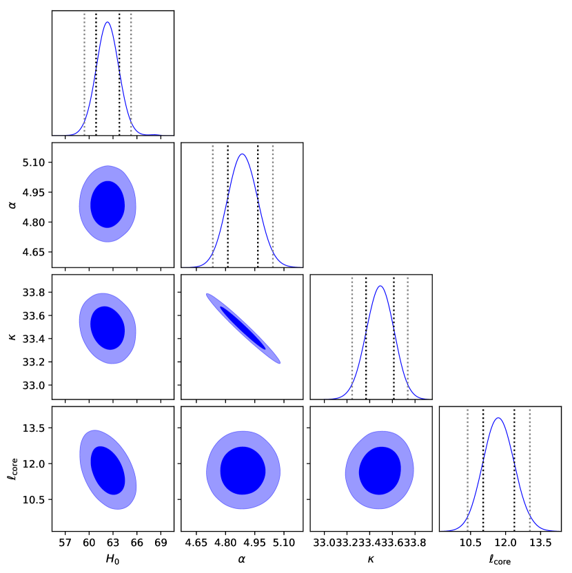
Figure 1: 1-2$\sigma$ confidence regions of the parameters $H_{0}$, $\alpha$, $\kappa$, and $\ell_{\rm core}$ for the $R_{\rm h}=ct$ Universe, along with their probability distributions.

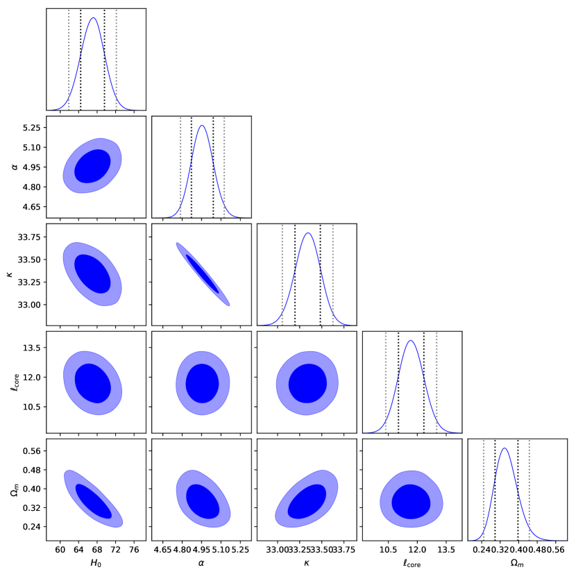
Figure 2: 1-D probability distributions and 2-D regions with 1-2$\sigma$ contours for the parameters $H_{0}$, $\alpha$, $\kappa$, $\ell_{\rm core}$, and $\Omega_{\rm m}$ for flat $\Lambda$CDM.

From the resulting model-specific likelihood function $\mathcal{L}_{\rm joint}$, which may also be viewed as a Bayesian posterior, we optimize the parameters by maximizing over their joint space. Such a procedure can be biased, so to avoid this, we also consider the shape of the function $\mathcal{L}_{\rm joint}$ near its maximum, as described below.

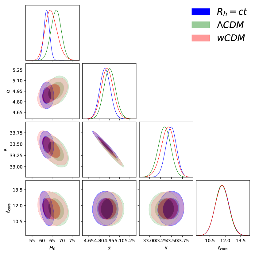
Figure 4: A comparison of the probability distributions and 1-2$\sigma$ confidence regions for $H_{0}$, $\alpha$, $\kappa$, and $\ell_{\rm core}$, for all three models.

In addition to optimizing these parameters by maximizing $\mathcal{L}_{\rm joint}$, we treat this joint likelihood function in a Bayesian fashion as an unnormalized probability density function on the joint parameter space, including the coefficients $\alpha$ and $\kappa$, and employ the pure-Python implementation of an affine invariant Markov chain Monte Carlo (MCMC) ensemble sampler called emcee [59] to generate a large random sample of points from this space, distributed according to the probability density function. This procedure allows us to determine the 1-D probability distributions and 2-D confidence regions with 1-2$\sigma$ contours for all the free parameters in each model, and these are shown in Figs. 1-3, along with a comparison for all three models in Fig. 4.

In statistics, the Bayesian information criterion (BIC) is commonly used for model selection among a finite set of models. The BIC is formally defined as

$$\mathrm{BIC}=k\ln(n)-2\ln(\mathcal{L}_{\rm joint}),$$ (19)

where $k$ is the number of free parameters and $n$ is the number of data points. According to [43], in a comparison between three cosmologies, model $\alpha$ has a likelihood

$$\mathcal{L}_{\alpha}=\frac{\exp(-\rm BIC_{\alpha}/2)}{\exp(-\rm BIC_{1}/2)+\exp(-\rm BIC_{2}/2)+\exp(-\rm BIC_{3}/2)}$$ (20)

of being the best choice. The best-fit values of the free parameters in each model, the BIC value for the optimized fit, and the corresponding probabilities, are listed in Table 2.

The use of the BIC is especially motivated when the samples are very large [43], which approximates the computation of the (logarithm of the) ‘Bayes factor’ for deciding between models [60, 61]. It is important to emphasize here that in the limit of large sample size $n$, particularly when $n\gg k$, the posterior distribution typically becomes increasingly peaked and Gaussian in shape. Kass & Raftery [61] used this property to justify the BIC, which is often cited in the statistics literature. As long as the parameters have a unimodal distribution that is roughly Gaussian, which turns out to be the case for the analysis in this paper, the Bayes factor between competing models can be calculated to high accuracy from the ratio of their respective (maximized) likelihoods. In the Kass & Raftery argument, the definite integrals of increasingly peaked integrands are approximated using Laplace’s method, similar to Stirling’s approach of calculating an asymptotic approximation to $n!$ when $n\gg 1$, as seen in his well-known formula. For the samples we use here, $n\gg 1$, which is deep in the asymptotic regime.

From Equation (20), we thus recognize an obvious Bayesian interpretation: $\exp(-{\rm BIC}_{\alpha}/2)$ is a large-sample $(n\to\infty)$ approximation to an integral over the joint parameter space of model $\alpha$, of its joint likelihood function $\mathcal{L}_{\rm joint}$. This integral could be evaluated by brute-force numerical calculations in low-dimensional cases. But to see that our approximation here is reasonable, suppose that $\mathcal{L}_{\rm joint}$ is Gaussian near its maximum, where it equals $\mathcal{L}^{*}_{\rm joint}$, and the $k$ parameters, called $\theta_{1},\dots\theta_{k}$ for the moment, statistically decouple. Then

$$\mathcal{L}_{\rm joint}\approx\mathcal{L}_{\rm joint}^{*}\exp\left[-\sum_{i=1}^{k}\frac{(\theta_{i}-\hat{\theta}_{i})^{2}}{2\sigma_{i}^{2}}\right]\;,$$ (21)

where $\sigma_{i}$ is the standard error of the estimate $\hat{\theta}_{i}$. Our integration of $\mathcal{L}_{\rm joint}$ over the $k$-dimensional parameter space yields $\mathcal{L}^{*}_{\rm joint}\prod_{i=1}^{k}\left(\sqrt{2\pi}\sigma_{i}\right)$. When the sample is very large, each $\sigma_{i}$ shrinks like $n^{-1/2}$, giving rise to an $n^{-k/2}$ factor, as seen in Eq. (19), which may equivalently be written

$$\exp(-{\rm BIC}/2)\equiv n^{-k/2}\mathcal{L}^{*}_{\rm joint}\;.$$ (22)

This is the reason why many data sets being analyzed today in cosmology utilize the BIC, which comes from Bayesian statistical inference, approximating the outcome of a Bayesian procedure for deciding between models, with an accuracy that improves with increasing $n$. The precision typically becomes very high when $n\gg k$, as we have in this paper [60, 61].

Table 2: Model Selection Based on the Joint Analysis of $H(z)$, HII-Galaxy and Quasar-Core Data

Model	$H_{0}$	$\Omega_{\rm m}$	$w_{\Lambda}$	$\alpha$	$\kappa$	$\ell_{\rm core}$	BIC	Prob
	(km s-1 Mpc-1)					(pc)		$(\%)$
$R_{\rm h}=ct$	$62.336\pm 1.464$	–	–	$4.889\pm 0.077$	$33.491\pm 0.123$	$11.709\pm 0.667$	$611.1228$	$96.7$
$\Lambda$CDM	$67.013\pm 2.578$	$0.347\pm 0.049$	$-1$ (fixed)	$4.956\pm 0.085$	$33.340\pm 0.143$	$11.684\pm 0.659$	$617.9843$	$3.1$
$w$CDM	$64.718\pm 3.088$	$0.247\pm 0.108$	$-0.693\pm 0.276$	$4.922\pm 0.088$	$33.415\pm 0.154$	$11.700\pm 0.665$	$623.4201$	$0.2$

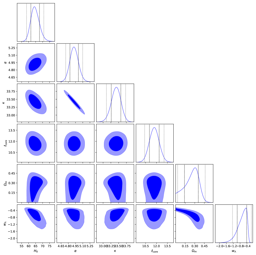
Figure 3: 1-2$\sigma$ constraints on $H_{0}$, $\alpha$, $\kappa$, $\ell_{\rm core}$, $\Omega_{\rm m}$, and $w_{\Lambda}$ for the flat $w$CDM model.

5 Discussion

A joint analysis allows us to obtain the best-fit results for more free parameters than are available when using a single data set. For example, when using just the measurements of $H(z)$, the optimization in $R_{\rm h}=ct$ yields just the value of $H_{0}$ [43]. With the combined analysis, the value of $H_{0}$ must be rendered consistently with all three data sets and the other variables, such as $\alpha$, $\kappa$, and $\ell_{\rm core}$. While the additional variables offer added flexibility, the fact that critical parameters, such as $H_{0}$, must optimize the fits of diverse data sets yields a tighter constraint on the model itself. An important outcome of our work is a demonstration that $H_{0}$ evaluated in this fashion is fully consistent (to within 1$\sigma$) with previously optimized values of the Hubble constant based on the analysis of single data sets [43, 46]. An additional benefit of using a joint analysis, e.g., with $H(z)$ and HII galaxies, is that one can separate the optimization of $\kappa$ and $H_{0}$, which is otherwise not possible using just the HII galaxies by themselves [46].

Our analysis in this paper has used three very different kinds of measurement: the expansion rate, the angular-diameter distance, and the luminosity distance, of diverse sources, so the fact that the optimized results are self-consistent provides a more compelling conclusion regarding the suitability and viability of the cosmological models. It is one thing to demonstrate consistency with one observational signature at a time, but when three different signatures are shown to be consistent with a single set of optimized parameters, principally $H_{0}$, the result is much more compelling. The optimized value of $H_{0}$ in $R_{\rm h}=ct$ is fully consistent with all 4 previous measurements of this constant [43, 34, 20, 42], i.e., $\sim 63$ km s^-1 Mpc^-1.

Likewise, the inferred values of $\Omega_{\rm m}$ and $w_{\rm de}$ are consistent with their Planck optimizations to within 1$\sigma$ [62]. Perhaps more importantly, our inferred value of $H_{0}$, especially for $\Lambda$CDM, is much more consistent with the Planck optimization than the locally measured value using Cepheid variables [63]. This reinforces the view held by some workers that the difference between the high- and low-redshift measurements of $H_{0}$ is real and may be due to the effects of a local Hubble bubble that alters the dynamics of expansion within a distance of $\sim 300$ pc of us (corresponding to $z\lesssim 0.07$) [64].

6 Conclusion

The results of this joint analysis affirm the viability of the $R_{\rm h}=ct$ cosmology. The joint analysis favors this model with a significantly higher probability than the standard model, or its variant $w$CDM. Should $R_{\rm h}=ct$ eventually emerge as the correct cosmology, many important consequences would follow. Clearly, it represents a significant step forward in helping us to understand the nature of dark energy. For one thing, it could not be a cosmological constant. It would have to be dynamic, probably representing new physics beyond the standard model of particle physics.

Most importantly, $R_{\rm h}=ct$ does not have a horizon problem, so it does not need inflation. Given how difficult it has been to find a self-consistent and complete model of inflation even after 30 years since its introduction, the viability of $R_{\rm h}=ct$ may allow us to completely avoid this poorly understood phenomenon altogether, because it simply may have never happened.

This paper has affirmed the benefits of carrying out model selection based on the joint analysis of various, diverse kinds of data. This clearly calls for broadening the scope of this kind of work, with the inclusion of other observations at both low- and high-redshifts. Ideally, one would wish to include all of the available data in such a joint analysis, but this goal will require a great deal of effort. As we have discussed in this manuscript, the work reported here makes the first serious attempt beyond simpler comparative studies based solely on single data sets. We have included three distinct kinds of measurement here. The difficulty with this procedure, of course, is finding data that are completely model independent or, at least, using them in a way that does not bias one model over another. We are currently working towards that goal, and constructive steps are being taken going forward. The outcome of this expanded analysis will be reported elsewhere. For the time being, however, the results presented in this manuscript constitute a significant advance over previous model comparisons, promising even more compelling results from future work.

References

- [1] R. Jimenez & A. Loeb, Astrophys. J. 573 (2002) 37.
- [2] M. Moresco, L. Verde & L. Pozzetti et al., J. Cosmol. Astropart. Phys. 53 (2012) 012.
- [3] C. Blake, S. Brough & M. Colless et al., Mon. Not. R. Astron. Soc. 425 (2012) 405.
- [4] J. Melnick, M. Moles, R. Terlevich & J. M. Garcia-Pelayo, Mon. Not. R. Astron. Soc. 226 (1987) 849.
- [5] J. Melnick, R. Terlevich & M. Moles, Mon. Not. R. Astron. Soc. 235 (1988) 297.
- [6] O. Fuentes-Masip, C. Muñoz-Tuñón, H. O. Castañeda & G. Tenorio-Tagle, Astron. J. 120 (2000) 752.
- [7] J. Melnick, R. Terlevich & E. Terlevich, Mon. Not. R. Astron. Soc. 311 (2000) 629.
- [8] G. Bosch, E. Terlevich & R. Terlevich, Mon. Not. R. Astron. Soc. 329 (2002) 481.
- [9] E. Telles, in Astronomical Society of the Pacific Conference Series, Vol. 297, Star Formation Through Time, ed. E. Perez, R. M. Gonzalez Delgado, & G. Tenorio-Tagle (2003) 143.
- [10] E. R. Siegel, R. Guzmán & J. P. Gallego et al., Mon. Not. R. Astron. Soc. 356 (2005) 1117.
- [11] V. Bordalo & E. Telles, Astrophys. J. 735 (2011) 52.
- [12] M. Plionis, R. Terlevich & S. Basilakos et al., Mon. Not. R. Astron. Soc. 416 (2011) 2981.
- [13] D. Mania & B. Ratra, Phys. Lett. B 715 (2012) 9.
- [14] R. Chávez, E. Terlevich & R. Terlevich et al., Mon. Not. R. Astron. Soc. 425 (2012) L56.
- [15] R. Terlevich, E. Terlevich & J. Melnick et al., Mon. Not. R. Astron. Soc. 451 (2015) 3001.
- [16] L. I. Gurvits, K. I. Kellermann & S. Frey, Astron. Astrophys. 342 (1999) 378.
- [17] S. Cao, M. Biesiada, X. Zheng & Z.-H. Zhu Astrophys. J. 806 (2015) 66.
- [18] S. Cao, M. Biesiada & J. Jackson et al. J. Cosmol. Astropart. Phys. 2 (2017) 012.
- [19] S. Cao, X. Zheng & M. Biesiada et al., Astron. Astrophys. 606 (2017) A15.
- [20] J.-J. Wei, F. Melia & X.-F. Wu, Astrophys. J. 835 (2017) 270.
- [21] W. J. Percival & M. White, Mon. Not. R. Astron. Soc. 393 (2009) 297.
- [22] E. Macaulay, I. K. Wehus & H. K. Eriksen, Phys. Rev. Lett. 111 (2013) 161301.
- [23] A. Pavlov, O. Farooq & B. Ratra, Phys. Rev. D 90 (2014) 023006.
- [24] S. Alam, S. Ho & A. Silvestri, Mon. Not. R. Astron. Soc. 456 (2016) 3743.
- [25] J. A. Peacock, S. Cole & P. Norberg et al., Nature 410 (2001) 169.
- [26] L. Guzzo, M. Pierleoni & B. Meneux et al., Nature 451 (2008) 541.
- [27] N. P. Ross, J. da Ângela & T. Shanks et al., Mon. Not. R. Astron. Soc. 381 (2007) 573.
- [28] J. da Ângela, T. Shanks & S.-M. Croom et al., Mon. Not. R. Astron. Soc. 383 (2008) 565.
- [29] M. Viel, M. G. Haehnelt & V. Springel, Mon. Not. R. Astron. Soc. 354 (2004) 684.
- [30] M. Davis, A. Nusser & K. L. Masters et al., Mon. Not. R. Astron. Soc. 413 (201) 2906.
- [31] M. J. Hudson & S. J. Turnbull, Astrophys. J. Lett. 751 (2012) L30.
- [32] F. Melia, Astron. J. 147 (2014) 120.
- [33] F. Melia, Astrophys. J. 764 (2013) 72.
- [34] F. Melia & T. M. McClintock, Astron. J. 150 (2015) 119.
- [35] C. L. Steinhardt, P. Capak, D. Masters & J. S. Speagle, Astrophys. J. 824 (2016) 21.
- [36] M. K. Yennapureddy & F. Melia, Eur. Phys. J. C 78 (2018) 258.
- [37] F. Melia, Mon. Not. R. Astron. Soc. 382 (2007) 1917.
- [38] F. Melia & M. Abdelqader, Int. J. Mod. Phys. D 18 (2009) 1889.
- [39] F. Melia & A.S.H. Shevchuk, Mon. Not. R. Astron. Soc. 419 (2012) 2579.
- [40] F. Melia, Annals of Physics, in press (2019).
- [41] F. Melia, Mon. Not. R. Astron. Soc. 464 (2017) 1966.
- [42] F. Melia & M. K. Yennapureddy, J. Cosmol. Astropart. Phys. 2 (2018) 034.
- [43] F. Melia & R. S. Maier, Mon. Not. R. Astron. Soc. 432 (2013) 2669.
- [44] S.-L. Cao, X.-W. Duan, X.-L. Meng & T.-J. Zhang, The European Physical Journal C 78 (2018) 313.
- [45] C.-Z. Ruan, F. Melia, Y. Chen & T.-J. Zhang, Astrophys. J. 881 (2019) 137.
- [46] J.-J. Wei, X.-F. Wu & F. Melia, Mon. Not. R. Astron. Soc. 463 (2016) 1144.
- [47] D. K. Erb, C. C. Steidel & A. E. Shapley et al., Astrophys. J. 646 (2006) 107.
- [48] C. Hoyos, D. C. Koo & A. C. Phillips et al., Astrophys. J. Lett. 635 (2005) L21.
- [49] M. V. Maseda, A. van der Wel & H.-W. Rix et al., Astrophys. J. 791 (2014) 17.
- [50] D. Masters, P. McCarthy & B. Siana et al., Astrophys. J. 785 (2014) 153.
- [51] R. Chávez, R. Terlevich & E. Terlevich et al., Mon. Not. R. Astron. Soc. 442 (2014) 3565.
- [52] R. Chávez, M. Plionis, S. Basilakos, R. Terlevich, E. Terlevich, J. Melnick, F. Bresolin & A. L. González-Morán, Mon. Not. R. Astron. Soc. 462 (2016) 2431.
- [53] J. C. Jackson & A. L. Jannetta, J. Cosmol. Astropart. Phys. 11 (2006) 002.
- [54] R. A. Preston, D. D. Morabito & J. G. Williams et al., Astron. J. 90 (1985) 1599.
- [55] L. I. Gurvits, Astrophys. J. 425 (1994) 442.
- [56] R. G. Vishwakarma, Class. Quant. Grav. 18 (2001) 1159.
- [57] R. C. Santos & J.A.S. Lima, Phys. Rev. D 77 (2008) 083505.
- [58] F. Melia, Front. Phys. 12 (2017) 129802.
- [59] D. Foreman-Mackey, D. W. Hogg, D. Lang & J. Goodman, Publ. Astron. Soc. Pac. 125 (2013) 306.
- [60] G. Schwarz, Ann. Statist. 6 (1978) 461.
- [61] R. E. Kass & A. E. Raftery, J. Amer. Statist. Assoc. 90 (1995) 773.
- [62] Planck Collaboration et al., Astron. Astrophys. 594 (2016) A13.
- [63] A. G. Riess, L. Macri & S. Casertano et al., Astrophys. J. 730 (2011) 119.
- [64] V. Marra, L. Amendola, I. Sawicki & W. Valkenburg, PRL 110 (2013) 241305.
- [65] C. Zhang, H. Zhang & S. Yuan et al., Res. Astron. Astrophys. 14 (2014) 1221.
- [66] R. Jimenez, L. Verde, T. Treu & D. Stern, Astrophys. J. 593 (2003) 622.
- [67] J. Simon, L. Verde & R. Jimenez, Phys. Rev. D 71 (2005) 123001.
- [68] M. Moresco, L. Pozzetti & A. Cimatti et al., J. Cosmol. Astropart. Phys. 5 (2016) 014.
- [69] D. Stern, R. Jimenez & L. Verde, et al., J. Cosmol. Astropart. Phys. 2 (2010) 8.
- [70] M. Moresco, Mon. Not. R. Astron. Soc. Lett. 450 (2015) L16.