Cosmology with Recombination Spectrum

Abstract

Precision measurement of the cosmological recombination spectrum can provide an entire new window to look at the early universe. We aim to quantify the information hidden in the cosmological recombination spectrum and for this purpose we have developed a new code following the algorithm proposed in [1, 2]. Our code is closely based on the COSMOSPEC [3] code. We find, using Fisher information matrix and assuming that the foregrounds can be subtracted by using higher or lower frequency channels and spatial information, that going beyond the detection will need an experiment with sensitivity $25\times$ better compared to the proposed experiment PIXIE. Such an experiment will be able to measure the cosmological parameters with a precision that is competitive with the CMB anisotropy experiments. The best constrainted parameter is baryon energy density, $\Omega_{\rm b}$, which can be nailed down with incredible precision in principle. We also show that the shape of the hydrogen lines is connected to the speed of the hydrogen recombination, with the peaks of the recombination lines coinciding with the peak of the recombination rate. In general, the shape of the lines encodes information about the rate of recombination as a function of redshift.

1 Introduction

Observations of the temperature and polarization anisotropies of the cosmic microwave background (CMB) have made it possible to determine the physics of the early universe to a very high level of precision. The Planck CMB space mission [4, 5, 6] has already extracted almost all the critical information from the temperature anisotropies, and future missions like LiteBIRD[7] , CoRE[8], PICO[9] and CMB-Bharat have been proposed to obtain all the cosmological information in the CMB polarization anisotropies. However, there is a significant amount of information hidden in the spectral distortions of the nearly perfect blackbody spectrum of the CMB [10, 11, 12, 13]. Spectral distortions can be created due to energy injection in the early universe, at redshifts $z\lesssim 2\times 10^{6}$, resulting in $\mu-$type, $y-$type, $i$-type, or non-thermal relativistic distortions [14, 15, 16, 17, 18]. There are many unavoidable sources of spectral distortions in standard cosmology [14, 19] such as silk damping [11, 20, 21, 22, 23], y-distortion from the reionization era, and the cosmological recombination spectrum [24, 25, 26, 27, 28, 29, 30, 31, 32, 33, 34, 35, 36, 37, 38, 39, 40, 41, 42, 43, 44, 45, 46, 47, 48, 49, 50, 51, 52, 53, 54].

We will focus on the cosmological recombination spectrum in this paper. The primordial hydrogen and helium recombinations [24, 25] create few photons per atom [31], which lead to a small distortion of $\Delta I_{\nu}/I_{\nu}\approx 10^{-9}$ in the CMB, where $I_{\nu}$ is the blackbody CMB intensity and $\Delta I_{\nu}$ is the intensity of the recombination lines. The cosmological recombination spectrum contains a wealth of information and is in particular not constrained by the cosmic variance which limits the precision with which we can measure the cosmological parameters with CMB anisotropies. In particular, it may provide an excellent measurement of the primordial helium abundance, uncontaminated by stellar contributions. The recombination spectrum can also be a probe of non-standard energy injections such as dark-matter annihilations [51].

In 1991, the observations of the cosmic microwave background (CMB) spectrum with Cosmic Background Explorer-Far Infrared Absolute Spectrophotometer (COBE/FIRAS) [55] showed that the CMB spectrum is close to a perfect black-body, with fractional deviations less than few $\times 10^{-5}$. Unlike the CMB anisotropies, which have seen precision improve by many orders of magnitude, the measurement of the CMB spectrum has not been updated since then. However, over the last 25 years the technology has improved considerably [56]. In recent years, various missions have been proposed [57, 58] to measure CMB spectral distortions. These proposed instruments are expected to detect the spectral deviations of the order of $\Delta I_{\nu}/I_{\nu}\sim 10^{-8}$ to $10^{-9}$, i.e. 3 to 4-orders of magnitude improvement over COBE-FIRAS. With this kind of sensitivity, it is possible to detect the recombination lines if we can separate them from foreground emissions. Since the recombination spectrum is expected to be isotropic and it has a very characteristic shape, this separation from the foregrounds should be possible in principle[59], although a clear demonstration of how accurately we can measure the cosmological recombination spectrum is pending and will require new foreground separation algorithms to be developed.

In this paper, we will not tackle the difficult question of foreground separation but rather attempt to quantify the information content of the cosmological recombination spectrum. We will assume that the frequency range $30~{}{\rm GHz}\leq\nu\leq 600~{}{\rm GHz}$ can be cleaned of foregrounds using frequency channels at $\nu\leq 30~{}{\rm GHz}$ and $\nu\geq 600~{}{\rm GHz}$ as assumed in the PIXIE proposal [57]. We want to ask the question what is the minimum improvement of sensitivity that is needed over PIXIE type experiment in order for the cosmological recombination spectrum to be competitive with the CMB anisotropies for measurement of the cosmological parameters. We also want to ask, given net total sensitivity of the experiment, whether it is more advantageous to divide the frequency channels into finer resolution channels with smaller sensitivity in each channel, or whether we want to have broader channels with higher sensitivity in each channel. This question has practical implications for the design of future experiments, since increasing the frequency resolution in a PIXIE type experiment increases the physical size of the experiment [57]. We also want to explore the complementarity of the recombination spectrum with the CMB anisotropy spectrum.

Computing the recombination spectrum requires computation of the populations of the excited states at each redshift, finding out corresponding the photon emission or absorption and finally solving the radiative transfer equation. High-precision computation of spectra requires accounting for excited states up to principal quantum number $n_{\max}$ of a few hundred and resolving the angular momentum sub-states. With the standard multilevel atom method, this will require a large computational time [60, 31, 29, 32, 36, 35, 49]. We follow the effective conductance method developed by [2], which bypasses this computational problem by dividing the problem into two parts: the cosmology independent but computationally expensive part which only depends on atomic physics and temperature and the cosmology dependent but computationally inexpensive part. The cosmology independent part depends only on temperature and hence needs to be computed once and for all and tabulated as a function of matter and radiation temperature, to be used again and again as needed [2]. The cosmology dependent part needs to be calculated every time we change the cosmological parameters. However, computing this part is fast, and hence, the total computation time is much smaller resulting in a fast and precise multi-level code without any fudge factors.

We closely follow the implementation of COSMOSPEC and refer the reader to [3] for details. We briefly review the essential aspects of the calculation below.

2 Computation of the cosmological recombination spectrum

In the optically thin limit, and in the absence of any source, the occupation number or the phase-space density of photons, $I_{\nu}/\nu^{3}$ can be assumed to be conserved, ${\rm d}(I_{\nu}/\nu^{3}){\rm d}t=0$, where $I_{\nu}$ is the intensity, $t$ is the proper time, and the derivative is a total derivative. The only dependence on time of the intensity in this case is implicit and comes solely due to the redshifting of the photons due to the expansion of the Universe. The solution to the above equation in the expanding Universe gives a simple relation for the intensity observed at redshift $z^{\prime}$, relating it to intensity at an earlier redshift $z$,

$$I_{\nu}(z)=\left(\frac{\nu}{\nu^{\prime}}\right)^{3}I_{\nu^{\prime}}(z^{\prime}),.$$ (2.1)

where $\nu^{\prime}=\nu(1+z^{\prime})/(1+z)$ is the redshifted frequency at $z^{\prime}$. During the recombination era, ions and electrons recombine to form atoms, emitting bound-bound and free-bound transition photons in the process which form the recombination spectrum. These photons form the source term or the emissivity $j_{\nu}$ in the radiative transfer equation,

$$\frac{d}{dt}\left(\frac{I_{\nu}}{\nu^{3}}\right)=c\frac{j_{\nu}}{\nu^{3}}.$$ (2.2)

Our main goal is to calculate this emissivity during the recombination epoch.

2.1 The effective conductance method

In the original three level atom of [24, 25], only the first excited level of hydrogen ($n=2$) was resolved, and all higher levels were assumed to be in thermal equilibrium with the $n=2$ level. In the three-level atom, therefore, the only photon emission comes from de-excitation from $n=2$ to $n=1$ level. The $Ly-\alpha$ photons, produced in $2p-1s$ transition mostly get captured by the recombining neutral hydrogen atoms, due to the high optical depth of the line, and only a very small fraction escape. This makes the very weak $2s-1s$ double photon decay also very important. The $2s-1s$ channel contributes significantly to the recombination process and hence to the recombination spectrum [29, 45, 37, 40] and needs to be taken into account. In general, we need to take into account all allowed transitions between all excited levels as well as weak transitions, such as 2-photon decays, from excited states to the ground state in a multi-level atom. The effective multi-level approach [1] divides the excited levels of atoms into interface states, $i$, defined as the states from which direct transitions to the ground state are taken into account. The populations of these levels, $x_{i}$, are explicitly followed. All other states are interior states from which direct transitions to the ground state are not important or not allowed. The effective multilevel atom takes the effect of these interior states also into account almost exactly, without explicitly solving for these states.

The effective conductance method extends this approach to compute the cosmological recombination spectrum in an efficient manner [2]. This is accomplished by realizing that in Saha equilibrium, the net emission would be balanced by absorption. Therefore, the net emissivity, $j_{\nu}$, will depend only on the departure of the level populations from the Saha equilibrium. The effective multilevel atom of [1] only keeps track of the populations in the interface levels. It was realized in [2] that the departures from the Saha equilibrium of all levels $\Delta x_{n\ell}$, where $n,\ell$ are the quantum numbers of the level, including interior states can be solved in terms of the level populations of interface levels, without explicitly following all interior states. Thus the net transition rates between two levels are proportional to departure of interface states from equilibrium, $\Delta x_{i}$, with the constant of proportionality, the effective conductance, only a function of matter and radiation temperatures and atomic physics and does not depend on cosmology or the actual level populations. These effective conductances can therefore also be computed and tabulated once and for all. We refer the reader to [2] for more details.

2.2 He recombination and feedback

It is essential to model helium recombination to compute the spectral distortion due to total recombination precisely. Since the ionization energy of helium is greater than hydrogen, helium recombination happens at much higher redshift compared to hydrogen recombination. The photons from the He recombination were more energetic, and they had to travel a much higher distance compared to photons originated due to hydrogen recombination. The helium photons interact with hydrogen as well as He atoms. Since the number density of helium atoms is $\approx 8\%$ of that of hydrogen, the intensity of the helium recombination spectrum is also $\approx 8\%$ of that of hydrogen. Photons emitted during the recombination phases of helium can ionize and excite the hydrogen at a later time. He II recombination photons can affect HeI and hydrogen recombination and HeI recombination photons can affect hydrogen recombination. These ionizations and excitations change the recombination spectra. We followed [3] to compute and take into account feedback effects. We take He levels into account up to principle quantum number of 100.

3 Cosmology with the recombination spectrum

3.1 Comparison with the COSMOREC

To check the accuracy of our implementation of the recombination calculation we compare with the publicly available COSMOREC code. The COSMOREC code [61] computes the recombination history and has the option to resolve first few levels of hydrogen and helium. We have done detailed comparison of first 10 levels of hydrogen and first 5 levels of helium and found agreement at the level of few $\%$. We show the comparison of the population levels of excited hydrogen states as computed by COSMOREC[61] and our code in Fig. 1. for 3 excited hydrogen levels. The full recombination spectrum, including contribution from helium, is shown in Fig. 2.

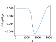
(a)

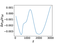
(b)

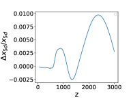
(c)

Figure 1: (a) The fractional difference between our code and COSMOREC for level populations, $\Delta x_{i}/x_{i}$: (a) 2p (b) 3d (c) 5d

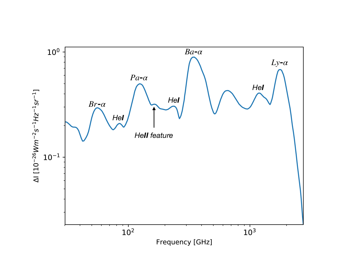
Figure 2: The cosmological recombination spectrum

3.2 Fisher Matrix analysis

Table 1: Experiment sensitivities for Fisher forecasts. For all experimental configurations we use the minimum and maximum frequency of $30~{}$GHz and $600~{}$GHz respectively. In addition for the same per channel sensitivity we consider 15GHz channels (same as PIXIE) and also 5GHz channels, effectively increasing the total sensitivity by $\sqrt{3}$ in the latter case over the former. We thus have total $39$ channels for 15GHz channel widths and $115$ channels for 5GHz channel widths. PIXIE sensitivity is shown just for reference.

Proposed Experiment	PIXIE	$25\times$ PIXIE	$\sqrt{3}\times 25\times$PIXIE	$100\times$ PIXIE
Sensitivity per channel ($Jy/sr$)	5	0.2	0.115	0.05

The Fisher information matrix for a series of independent data points/observables $f_{b}$, which are function of parameters $p_{i}$ with Gaussian uncertainties $\sigma_{b}$ for each data point is defined as

$$F_{jk}=\sum_{b}\frac{1}{\sigma_{b}^{2}}\frac{\partial f_{b}}{\partial p_{j}}\frac{\partial f_{b}}{\partial p_{k}}$$ (3.1)

The covariance matrix is the inverse of the Fisher matrix. The Fisher matrix provides a best-case scenario for the ability of a a set of experiments to constrain parameters. For our case, the observables are the recombination spectrum intensities in different frequency bands. The recombination spectrum is a function of the cosmological parameters the baryon density parameter ($\Omega_{b}$), the cold dark matter density parameter ($\Omega_{c}$), the mass fraction of helium ($Y_{p}$), the Hubble constant ($H_{0}$, $h\equiv H_{0}/100$), and the effect relativistic degrees of freedom ($N_{\rm eff}$). The Fisher matrix depends on the values of fiducial parameters where we evaluate the derivative. We use Planck 2018 [6] TT+lowE best fit parameters as our fiducial cosmology. The intensity in each frequency channel is an independent data point $b$. We also want to compare the forecasts with CMB anisotropy as well as give the combined forecasts for recombination spectrum and the CMB anisotropies to explore their complementarity. We use the Planck results as the reference case for the anisotropies, although we should expect improvements in anisotropy measurements, especially polarization anisotropies, with future experiments ^[1] [8, 9, 7] .We use the covariance matrix from the Planck Likelihood data from Planck Legacy Archive. For the joint forecast, the combined Fisher matrix is then just the sum of two Fisher matrices.

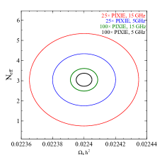
Figure 3: Marginalized 68 percent confidence constraints for $\Omega_{b}h^{2}$ and $N_{\rm eff}$ for different experiment configurations. We label the improvement in sensitivity per channel over PIXIE sensitivity per channel as $N\times$PIXIE. The minimum and maximum frequency channels are at $30$ and $600$ GHZ respectively. This given $39$ channels for 15GHz channel widths and $115$ channels for 5GHz channel widths.

To obtain the error ellipses for any subset of parameters, we need to marginalize the Fisher matrix. Let the full parameter set be represented by $\vec{i}$ and a subset we are interested in by $\vec{j}$ and the rest of parameters by $\vec{k}$. The Fisher matrix $F^{\prime}$ after marginalization over $\vec{k}$ can be expressed as,

$$F^{\prime}=F_{jj}-F_{jk}F^{-1}_{kk}F_{kj}$$ (3.2)

Inverting $F^{\prime}$ gives the marginalized covariance matrix for parameters of interest.

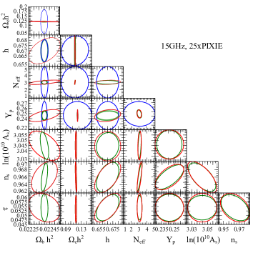
Figure 4: Constraints for a PIXIE type experiment with 15GHZ wide channels but $25\times$ more sensitivity per channel (blue). We also show constraints when combined with Planck (green) and Planck 2018 constraints (red).

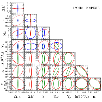
Figure 5: Same as Fig. 4 but with 15GHz channels and $100\times$PIXIE sensitivity per channel.

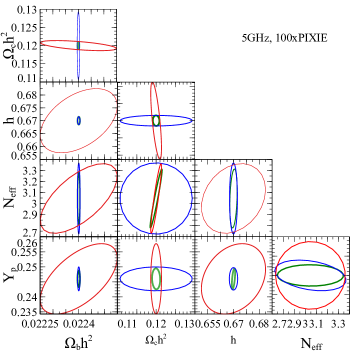
Figure 6: Same as Fig. 4 but with 5GHz channels and $100\times$PIXIE sensitivity per channel.

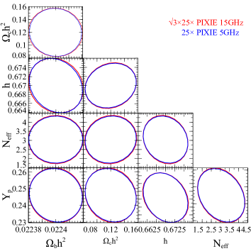
Figure 7: Same as Fig. 4 but with 5GHz channels and $25\times$PIXIE sensitivity and 15GHz channels and $\sqrt{3}\times 25\times$PIXIE per channel sensitivity.

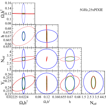
Figure 8: Same as Fig. 4 but with 5GHz channels and $25\times$PIXIE per channel sensitivity.

We consider several experiment configurations, shown in Table 1, with PIXIE [57] proposal as the reference. A PRISM-like [58] instrument with $\approx 8\times$ better sensitivity compared to PIXIE will be able to just detect the recombination spectrum. However we want to go beyond that and consider precision measurement of cosmological parameters from recombination spectrum. Therefore the minimum sensitivity of the experiments we consider is a factor of $25$ better compared to PIXIE. In principle, since there is no cosmic variance, we can keep on increasing the sensitivity until we are limited by the foregrounds. On the other hand, foregrounds can be subtracted more and more accurately by increasing the number of frequency channels. At the other extreme, we consider an ultra-futuristic experiment with $5~{}$GHz channels and a sensitivity per channel of $0.05~{}{\rm Jy/sr}$, i.e. $100\sqrt{3}$ times more combined sensitive than PIXIE. We will refer to per channel sensitivity everywhere with reference to PIXIE. Therefore, a 25XPIXIE experiment with 5GHZ channels has $\sqrt{3}$ better sensitivity compared to a 25XPIXIE experiment with 15GHz channels, assuming same minimum and maximum frequencies. The exact sensitivity values are given in Table 1.

The Fisher forecasts are shown in Figs. 4-8 as 2-parameter contour plots and in Tables 2 and 3 as 1-$\sigma$ expected errorbars on different parameters. We see that a factor of $25$ sensitivity would nail down the baryon density, giving a factor of 5 improvement over Planck. The cosmological recombination spectrum is less sensitive to the other cosmological parameters but in principle still deliver competitive constraints. In particular, it is possible to estimate helium fraction, and Hubble parameter and $h_{0}$ better than the Planck [4, 5, 6] but it will require sensitivity that is a factor of $100$ better compared to Planck. When combining with Planck, we see that there is small improvement in $N_{\rm eff}$ and Hubble parameter $h$ due to their small degeneracy with $\Omega_{b}h^{2}$. However, first and foremost, the cosmic recombination spectrum is a precise baryon-meter. There is almost no effect on the perturbative parameters, the amplitude of primordial curvature perturbation ($A_{\rm s}$), its spectral index ($n_{\rm s})$, and optical depth to reionization $\tau_{\rm ri}$. In general, any parameter which has degeneracy with baryon density would benefit from the cosmological recombination spectrum.

In Fig. 7 we compare two experiments with the same total combined sensitivity but different frequency resolution. The two experiments are almost indistinguishable indicating that the frequency resolution does not affect the precision of cosmological parameters. The frequency resolution of the experiment should therefore be determined by foreground cleaning requirements. In general, as the total sensitivity increases, we will need better foreground cleaning and hence better frequency resolution. We leave a detailed study of this very important aspect to future work.

Table 2: Constraints on standard cosmological parameters from Planck data and different experiment configurations defined in Table 1.

Parameters	Planck	$25\times$ PIXIE	Planck$+25\times$PIXIE	$100\times$ PIXIE	Planck$+100\times$PIXIE
$\Omega_{b}h^{2}$	$0.00015$	$0.000031$	$0.000031$	$0.00000707$	$0.00000706$
$\Omega_{c}h^{2}$	$0.0014$	$0.065$	$0.00138$	$0.01625$	$0.00135$
$N_{eff}$	$0.31$	$2.202$	$0.264$	$0.56$	$0.26$
$Y_{p}$	$0.0117$	$0.032$	$0.0089$	$0.0078$	$0.00547$
$h$	$0.012$	$0.0109$	$0.01$	$0.00271$	$0.00193$
$n_{\rm s}$	$0.0042$		$0.00398$		$0.00394$
$ln(10^{10}A_{\rm s})$	$0.014$		$0.0131$		$0.01305$
$\tau_{\rm ri}$	$0.0073$		$0.00706$		$0.007$

Table 3: Constraints on standard cosmological parameters from Planck data and different experiment configurations defined in Table 1.

Parameters	Planck	$25\times$ PIXIE	Planck$+25\times$PIXIE	$100\times$ PIXIE	Planck$+100\times$PIXIE
$\Omega_{b}h^{2}$	$0.00015$	$0.00001789$	$0.0000178$	$0.00000447$	$0.0000044$
$\Omega_{c}h^{2}$	$0.0014$	$0.0373$	$0.0012$	$0.0093$	$0.0011$
$N_{\rm eff}$	$0.31$	$1.29$	$0.29$	$0.32$	$0.25$
$Y_{p}$	$0.0117$	$0.0184$	$0.008$	$0.0045$	$0.0039$
$h$	$0.012$	$0.006293$	$0.006285$	$0.00153$	$0.00152$
$n_{\rm s}$	$0.0042$		$0.00396$		$0.00394$
$ln(10^{10}A_{\rm s})$	$0.014$		$0.01301$		$0.013$
$\tau_{\rm ri}$	$0.0073$		$0.007$		$0.007$

3.3 The shape and position of the lines

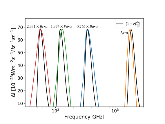
Figure 9: Comparison of our simple ansatz for the shape of the recombination lines (Eq. 3.5) with the actual line shapes.

The rate of change of electron fraction $x_{\rm e}$ and recombination spectrum are expected to be closely related to each other. We would expect in general that a faster recombination at a particular redshift would produce more recombination photons for every line at the corresponding redshifted observed frequency. This leads us to postulate a simple ansatz for the shape of the recombination lines. Let us assume that the net transition rate per unit volume $\Delta R(z)$ at any line is just proportional to the recombination rate, $\Delta R(z)\propto n_{\rm H}\frac{dx_{\rm e}}{dt}$, where $n_{\rm H}$ is the total hydrogen number density. The intensity in a recombination line is given by [33, 30]

$$I_{\nu}=\frac{ch}{4\pi}\frac{\Delta R(z)}{H(1+z)^{3}}$$ (3.3)

Putting $\Delta R(z)\propto n_{\rm H}\frac{dx_{\rm e}}{dt}$, the line shape is given by

$$I_{\nu}=A(1+z)\frac{dx_{\rm e}}{dz},$$ (3.5)

where $A$ is the normalization which is different for every line. We compare the intensity calculated with this ansatz, after fitting the amplitude $A$ so that the lines have the same normalization, in Fig 9. Note that we need to relate the observed frequency with the redshift as

$$(1+z)=\frac{\nu_{em}}{\nu_{obs}},$$ (3.6)

where, $\nu_{em}$ and $\nu_{obs}$ are the emitted and observed frequencies of the line respectively. We see from Fig. 9 that the above very simple ansatz gets the peak of line position right for the Balmer and Brackett lines, and quite close for the Lyman and Paschen lines. The line width is close for the Lyman-$\alpha$ line but underestimated by our ansatz for the other lines. However in general the line shapes are similar enough and this gives support to the idea that the recombination spectrum carries detailed information about the whole history of recombination compared to the integrated effect of the visibility function that we are sensitive to with the CMB anisotropies. This is particularly important if we want to constrain new physics which modifies the recombination history but without significant effect on the visibility function. We leave exploration of such scenarios to future work.

4 Conclusions

Cosmological recombination spectrum promises to provide an exciting new window to look at the early universe, one that is not limited by cosmic variance and can therefore result in unprecedented precision for the measurement of standard cosmological parameters. This will be an independent measurement of the cosmological parameters. Improvement of precision in independent probes is of tremendous importance, as it may uncover new anomalies which may point to the new physics beyond the standard model.

The quantification of the information content of the cosmological recombination spectrum and how to extract it from data in the presence of foreground, are both very important questions for building the science case and designing future missions [62]. We have tried to answer the first question in this paper and leave exploration of the second question to future work.

References

- [1] Y. Ali-Haimoud and C. M. Hirata, Ultrafast effective multi-level atom method for primordial hydrogen recombination, Phys. Rev. D82 (2010) 063521 [1006.1355].
- [2] Y. Ali-Haïmoud, Effective conductance method for the primordial recombination spectrum, Phys. Rev. D 87 (2013) 023526 [1211.4031].
- [3] J. Chluba and Y. Ali-Haïmoud, COSMOSPEC: fast and detailed computation of the cosmological recombination radiation from hydrogen and helium, MNRAS 456 (2016) 3494 [1510.03877].
- [4] Planck Collaboration, P. A. R. Ade, N. Aghanim, C. Armitage-Caplan, M. Arnaud, M. Ashdown et al., Planck 2013 results. XVI. Cosmological parameters, A&A 571 (2014) A16 [1303.5076].
- [5] Planck Collaboration, P. A. R. Ade, N. Aghanim, M. Arnaud, M. Ashdown, J. Aumont et al., Planck 2015 results. XIII. Cosmological parameters, A&A 594 (2016) A13 [1502.01589].
- [6] Planck Collaboration, N. Aghanim, Y. Akrami, M. Ashdown, J. Aumont, C. Baccigalupi et al., Planck 2018 results. VI. Cosmological parameters, arXiv e-prints (2018) arXiv:1807.06209 [1807.06209].
- [7] T. Matsumura, Y. Akiba, J. Borrill, Y. Chinone, M. Dobbs, H. Fuke et al., Mission Design of LiteBIRD, Journal of Low Temperature Physics 176 (2014) 733 [1311.2847].
- [8] CORE collaboration, Exploring cosmic origins with CORE: Survey requirements and mission design, JCAP 1804 (2018) 014 [1706.04516].
- [9] S. Hanany, M. Alvarez, E. Artis, P. Ashton, J. Aumont, R. Aurlien et al., PICO: Probe of Inflation and Cosmic Origins, arXiv e-prints (2019) arXiv:1908.07495 [1908.07495].
- [10] Y. B. Zeldovich and R. A. Sunyaev, The Interaction of Matter and Radiation in a Hot-Model Universe, Ap&SS 4 (1969) 301.
- [11] R. A. Sunyaev and Y. B. Zeldovich, The interaction of matter and radiation in the hot model of the Universe, II, Ap&SS 7 (1970) 20.
- [12] A. F. Illarionov and R. A. Siuniaev, Comptonization, the background-radiation spectrum, and the thermal history of the universe, Soviet Ast. 18 (1975) 691.
- [13] L. Danese and G. de Zotti, Double Compton process and the spectrum of the microwave background, A&A 107 (1982) 39.
- [14] J. Chluba and R. A. Sunyaev, The evolution of CMB spectral distortions in the early Universe, Mon. Not. Roy. Astron. Soc. 419 (2012) 1294 [1109.6552].
- [15] R. Khatri and R. A. Sunyaev, Beyond y and : the shape of the CMB spectral distortions in the intermediate epoch, z , J. Cosmology Astropart. Phys 9 (2012) 016 [1207.6654].
- [16] J. Chluba, Green’s function of the cosmological thermalization problem, MNRAS 434 (2013) 352 [1304.6120].
- [17] S. K. Acharya and R. Khatri, Rich structure of nonthermal relativistic CMB spectral distortions from high energy particle cascades at redshifts , Phys. Rev. D 99 (2019) 043520 [1808.02897].
- [18] S. K. Acharya and R. Khatri, New CMB spectral distortion constraints on decaying dark matter with full evolution of electromagnetic cascades before recombination, Phys. Rev. D 99 (2019) 123510 [1903.04503].
- [19] R. A. Sunyaev and R. Khatri, Unavoidable CMB Spectral Features and Blackbody Photosphere of Our Universe, International Journal of Modern Physics D 22 (2013) 1330014 [1302.6553].
- [20] R. A. Daly, Spectral distortions of the microwave background radiation resulting from the damping of pressure waves, ApJ 371 (1991) 14.
- [21] W. Hu, D. Scott and J. Silk, Power Spectrum Constraints from Spectral Distortions in the Cosmic Microwave Background, ApJ 430 (1994) L5 [astro-ph/9402045].
- [22] J. Chluba, R. Khatri and R. A. Sunyaev, CMB at order: the dissipation of primordial acoustic waves and the observable part of the associated energy release, MNRAS 425 (2012) 1129.
- [23] R. Khatri, R. A. Sunyaev and J. Chluba, Mixing of blackbodies: entropy production and dissipation of sound waves in the early Universe, A&A 543 (2012) A136.
- [24] Y. B. Zel’dovich, V. G. Kurt and R. A. Syunyaev, Recombination of Hydrogen in the Hot Model of the Universe, Soviet Journal of Experimental and Theoretical Physics 28 (1969) 146.
- [25] P. J. E. Peebles, Recombination of the Primeval Plasma, ApJ 153 (1968) 1.
- [26] V. K. Dubrovich, Hydrogen recombination lines of cosmological origin, Soviet Astronomy Letters 1 (1975) 196.
- [27] S. Seager, D. D. Sasselov and D. Scott, How Exactly Did the Universe Become Neutral?, ApJS 128 (2000) 407.
- [28] V. K. Dubrovich and S. I. Grachev, Recombination Dynamics of Primordial Hydrogen and Helium (He I) in the Universe, Astronomy Letters 31 (2005) 359.
- [29] J. Chluba and R. A. Sunyaev, Induced two-photon decay of the 2s level and the rate of cosmological hydrogen recombination, A&A 446 (2006) 39.
- [30] J. A. Rubiño-Martín, J. Chluba and R. A. Sunyaev, Lines in the cosmic microwave background spectrum from the epoch of cosmological hydrogen recombination, MNRAS 371 (2006) 1939.
- [31] J. Chluba and R. A. Sunyaev, Free-bound emission from cosmological hydrogen recombination, A&A 458 (2006) L29.
- [32] E. E. Kholupenko and A. V. Ivanchik, Two-photon 2s 1s transitions during hydrogen recombination in the universe, Astronomy Letters 32 (2006) 795.
- [33] W. Y. Wong, S. Seager and D. Scott, Spectral distortions to the cosmic microwave background from the recombination of hydrogen and helium, MNRAS 367 (2006) 1666 [astro-ph/0510634].
- [34] W. Y. Wong and D. Scott, The effect of forbidden transitions on cosmological hydrogen and helium recombination, MNRAS 375 (2007) 1441.
- [35] J. Chluba, J. A. Rubiño-Martín and R. A. Sunyaev, Cosmological hydrogen recombination: populations of the high-level substates, MNRAS 374 (2007) 1310 [astro-ph/0608242].
- [36] J. Chluba and R. A. Sunyaev, Cosmological hydrogen recombination: Lyn line feedback and continuum escape, A&A 475 (2007) 109 [astro-ph/0702531].
- [37] C. M. Hirata, Two-photon transitions in primordial hydrogen recombination, Phys. Rev. D 78 (2008) 023001.
- [38] S. G. Karshenboim and V. G. Ivanov, Nonresonant effects and hydrogen transition line shape in cosmological recombination problems, Astronomy Letters 34 (2008) 289.
- [39] E. R. Switzer and C. M. Hirata, Primordial helium recombination. I. Feedback, line transfer, and continuum opacity, Phys. Rev. D 77 (2008) 083006.
- [40] C. M. Hirata and E. R. Switzer, Primordial helium recombination. II. Two-photon processes, Phys. Rev. D 77 (2008) 083007 [astro-ph/0702144].
- [41] E. R. Switzer and C. M. Hirata, Primordial helium recombination. III. Thomson scattering, isotope shifts, and cumulative results, Phys. Rev. D 77 (2008) 083008 [astro-ph/0702145].
- [42] S. I. Grachev and V. K. Dubrovich, Primordial hydrogen recombination dynamics with recoil upon scattering in the Ly- line, Astronomy Letters 34 (2008) 439 [0801.3347].
- [43] E. E. Kholupenko, A. V. Ivanchik and D. A. Varshalovich, He II He I recombination of primordial helium plasma including the effect of neutral hydrogen, Astronomy Letters 34 (2008) 725 [0812.3067].
- [44] J. A. Rubiño-Martín, J. Chluba and R. A. Sunyaev, Lines in the cosmic microwave background spectrum from the epoch of cosmological helium recombination, A&A 485 (2008) 377.
- [45] J. Chluba and R. A. Sunyaev, Two-photon transitions in hydrogen and cosmological recombination, A&A 480 (2008) 629.
- [46] J. Chluba and R. A. Sunyaev, Time-dependent corrections to the Ly escape probability during cosmological recombination, A&A 496 (2009) 619 [0810.1045].
- [47] C. M. Hirata and J. Forbes, Lyman- transfer in primordial hydrogen recombination, Phys. Rev. D 80 (2009) 023001 [0903.4925].
- [48] J. Chluba and R. A. Sunyaev, Cosmological hydrogen recombination: influence of resonance and electron scattering, A&A 503 (2009) 345 [0904.2220].
- [49] J. Chluba and R. A. Sunyaev, Cosmological recombination: feedback of helium photons and its effect on the recombination spectrum, MNRAS 402 (2010) 1221.
- [50] J. Chluba and R. A. Sunyaev, Ly escape during cosmological hydrogen recombination: the 3d-1s and 3s-1s two-photon processes, A&A 512 (2010) A53 [0904.0460].
- [51] J. Chluba, Could the cosmological recombination spectrum help us understand annihilating dark matter?, MNRAS 402 (2010) 1195 [0910.3663].
- [52] D. Grin and C. M. Hirata, Cosmological hydrogen recombination: The effect of extremely high-n states, Phys. Rev. D 81 (2010) 083005.
- [53] Y. Ali-Haïmoud, D. Grin and C. M. Hirata, Radiative transfer effects in primordial hydrogen recombination, Phys. Rev. D 82 (2010) 123502 [1009.4697].
- [54] J. Chluba, J. Fung and E. R. Switzer, Radiative transfer effects during primordial helium recombination, MNRAS 423 (2012) 3227 [1110.0247].
- [55] D. J. Fixsen, E. S. Cheng, J. M. Gales, J. C. Mather, R. A. Shafer and E. L. Wright, The Cosmic Microwave Background Spectrum from the Full COBE FIRAS Data Set, ApJ 473 (1996) 576 [astro-ph/9605054].
- [56] D. J. Fixsen and J. C. Mather, The Spectral Results of the Far-Infrared Absolute Spectrophotometer Instrument on COBE, ApJ 581 (2002) 817.
- [57] A. Kogut, D. J. Fixsen, D. T. Chuss, J. Dotson, E. Dwek, M. Halpern et al., The Primordial Inflation Explorer (PIXIE): a nulling polarimeter for cosmic microwave background observations, J. Cosmology Astropart. Phys 2011 (2011) 025 [1105.2044].
- [58] P. André, C. Baccigalupi, A. Banday, D. Barbosa, B. Barreiro, J. Bartlett et al., PRISM (Polarized Radiation Imaging and Spectroscopy Mission): an extended white paper, J. Cosmology Astropart. Phys 2014 (2014) 006 [1310.1554].
- [59] M. Sathyanarayana Rao, R. Subrahmanyan, N. Udaya Shankar and J. Chluba, On the Detection of Spectral Ripples from the Recombination Epoch, ApJ 810 (2015) 3 [1501.07191].
- [60] S. Seager, D. D. Sasselov and D. Scott, A New Calculation of the Recombination Epoch, ApJ 523 (1999) L1 [astro-ph/9909275].
- [61] J. Chluba and R. M. Thomas, Towards a complete treatment of the cosmological recombination problem, MNRAS 412 (2011) 748 [1010.3631].
- [62] J. Chluba, M. H. Abitbol, N. Aghanim, Y. Ali-Haimoud, M. Alvarez, K. Basu et al., New Horizons in Cosmology with Spectral Distortions of the Cosmic Microwave Background, arXiv e-prints (2019) arXiv:1909.01593 [1909.01593].