Learning-Based Low-Rank Approximations

Abstract

We introduce a “learning-based” algorithm for the low-rank decomposition problem: given an $n\times d$ matrix $A$, and a parameter $k$, compute a rank-$k$ matrix $A^{\prime}$ that minimizes the approximation loss $\|A-A^{\prime}\|_{F}$. The algorithm uses a training set of input matrices in order to optimize its performance. Specifically, some of the most efficient approximate algorithms for computing low-rank approximations proceed by computing a projection $SA$, where $S$ is a sparse random $m\times n$ “sketching matrix”, and then performing the singular value decomposition of $SA$. We show how to replace the random matrix $S$ with a “learned” matrix of the same sparsity to reduce the error.

Our experiments show that, for multiple types of data sets, a learned sketch matrix can substantially reduce the approximation loss compared to a random matrix $S$, sometimes by one order of magnitude. We also study mixed matrices where only some of the rows are trained and the remaining ones are random, and show that matrices still offer improved performance while retaining worst-case guarantees.

Finally, to understand the theoretical aspects of our approach, we study the special case of $m=1$. In particular, we give an approximation algorithm for minimizing the empirical loss, with approximation factor depending on the stable rank of matrices in the training set. We also show generalization bounds for the sketch matrix learning problem.

1 Introduction

The success of modern machine learning made it applicable to problems that lie outside of the scope of “classic AI”. In particular, there has been a growing interest in using machine learning to improve the performance of “standard” algorithms, by fine-tuning their behavior to adapt to the properties of the input distribution, see e.g., (Wang et al., 2016; Khalil et al., 2017; Kraska et al., 2018; Balcan et al., 2018; Lykouris and Vassilvitskii, 2018; Purohit et al., 2018; Gollapudi and Panigrahi, 2019; Mitzenmacher, 2018; Mousavi et al., 2015; Baldassarre et al., 2016; Bora et al., 2017; Metzler et al., 2017; Hand and Voroninski, 2018; Khani et al., 2019; Hsu et al., 2019). This “learning-based” approach to algorithm design has attracted a considerable attention over the last few years, due to its potential to significantly improve the efficiency of some of the most widely used algorithmic tasks. Many applications involve processing streams of data (video, data logs, customer activity etc) by executing the same algorithm on an hourly, daily or weekly basis. These data sets are typically not “random” or “worst-case”; instead, they come from some distribution which does not change rapidly from execution to execution. This makes it possible to design better algorithms tailored to the specific data distribution, trained on past instances of the problem.

The method has been particularly successful in the context of compressed sensing. In the latter framework, the goal is to recover an approximation to an $n$-dimensional vector $x$, given its “linear measurement” of the form $Sx$, where $S$ is an $m\times n$ matrix. Theoretical results (Donoho, 2006; Candès et al., 2006) show that, if the matrix $S$ is selected at random, it is possible to recover the $k$ largest coefficients of $x$ with high probability using a matrix $S$ with $m=O(k\log n)$ rows. This guarantee is general and applies to arbitrary vectors $x$. However, if vectors $x$ are selected from some natural distribution (e.g., they represent images), recent works (Mousavi et al., 2015; Baldassarre et al., 2016; Metzler et al., 2017) show that one can use samples from that distribution to compute matrices $S$ that improve over a completely random matrix in terms of the recovery error.

Compressed sensing is an example of a broader class of problems which can be solved using random projections. Another well-studied problem of this type is low-rank decomposition: given an $n\times d$ matrix $A$, and a parameter $k$, compute a rank-$k$ matrix

$$[A]_{k}=\mbox{argmin}_{A^{\prime}:\mbox{~{}rank}(A^{\prime})\leq k}\|A-A^{\prime}\|_{F}.$$

Low-rank approximation is one of the most widely used tools in massive data analysis, machine learning and statistics, and has been a subject of many algorithmic studies. In particular, multiple algorithms developed over the last decade use the “sketching” approach, see e.g., (Sarlos, 2006; Woolfe et al., 2008; Halko et al., 2011; Clarkson and Woodruff, 2009, 2017; Nelson and Nguyên, 2013; Meng and Mahoney, 2013; Boutsidis and Gittens, 2013; Cohen et al., 2015). Its idea is to use efficiently computable random projections (a.k.a., “sketches”) to reduce the problem size before performing low-rank decomposition, which makes the computation more space and time efficient. For example, (Sarlos, 2006; Clarkson and Woodruff, 2009) show that if $S$ is a random matrix of size $m\times n$ chosen from an appropriate distribution, for $m$ depending on $\varepsilon$, then one can recover a rank-$k$ matrix $A^{\prime}$ such that

$$\|A-A^{\prime}\|_{F}\leq(1+\epsilon)\|A-[A]_{k}\|_{F}$$

by performing an SVD on $SA\in\mathbb{R}^{m\times d}$ followed by some post-processing. Typically the sketch length $m$ is small, so the matrix $SA$ can be stored using little space (in the context of streaming algorithms) or efficiently communicated (in the context of distributed algorithms). Furthermore, the SVD of $SA$ can be computed efficiently, especially after another round of sketching, reducing the overall computation time. See the survey (Woodruff, 2014) for an overview of these developments.

In light of the aforementioned work on learning-based compressive sensing, it is natural to ask whether similar improvements in performance could be obtained for other sketch-based algorithms, notably for low-rank decompositions. In particular, reducing the sketch length $m$ while preserving its accuracy would make sketch-based algorithms more efficient. Alternatively, one could make sketches more accurate for the same values of $m$. This is the problem we address in this paper.

Our Results.

Our main finding is that learned sketch matrices can indeed yield (much) more accurate low-rank decompositions than purely random matrices. We focus our study on a streaming algorithm for low-rank decomposition due to (Sarlos, 2006; Clarkson and Woodruff, 2009), described in more detail in Section 2. Specifically, suppose we have a training set of matrices $\mathsf{Tr}=\{A_{1},\ldots,A_{N}\}$ sampled from some distribution $\mathcal{D}$. Based on this training set, we compute a matrix $S^{*}$ that (locally) minimizes the empirical loss

$$\sum_{i}\|A_{i}-\mathrm{SCW}(S^{*},A_{i})\|_{F}$$ (1.1)

where $\mathrm{SCW}(S^{*},A_{i})$ denotes the output of the aforementioned Sarlos-Clarkson-Woodruff streaming low-rank decomposition algorithm on matrix $A_{i}$ using the sketch matrix $S^{*}$. Once the sketch matrix $S^{*}$ is computed, it can be used instead of a random sketch matrix in all future executions of the SCW algorithm.

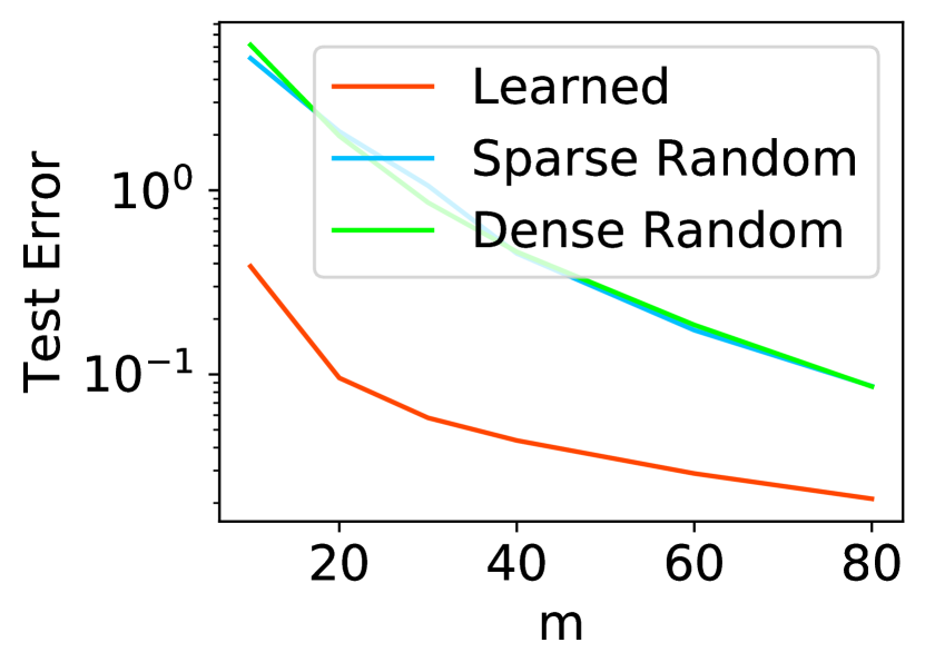
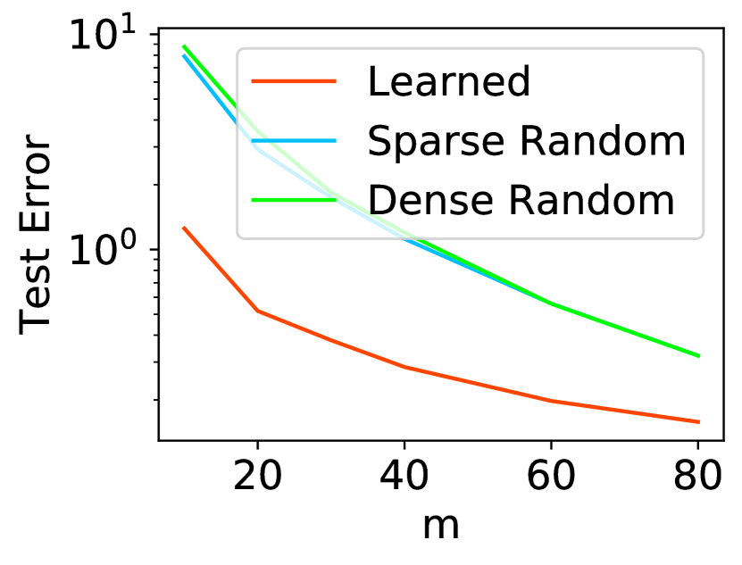
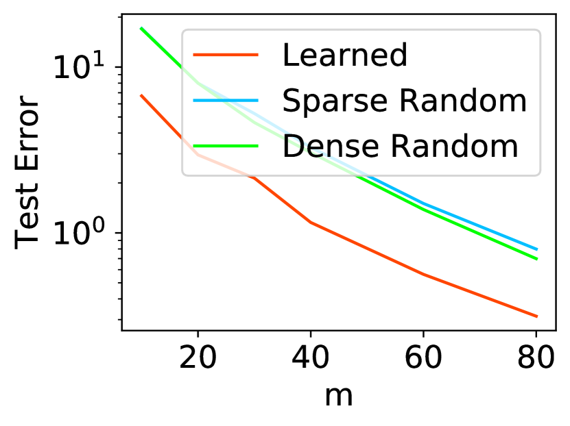
We demonstrate empirically that, for multiple types of data sets, an optimized sketch matrix $S^{*}$ can substantially reduce the approximation loss compared to a random matrix $S$, sometimes by one order of magnitude (see Figure 5.1 or 5.2). Equivalently, the optimized sketch matrix can achieve the same approximation loss for lower values of $m$ which results in sketching matrices with lower space usage. Note that since we augment a streaming algorithm, our main focus is on improving its space usage (which in the distributed setting translates into the amount of communication). The latter is $O(md)$, the size of $SA$.

A possible disadvantage of learned sketch matrices is that an algorithm that uses them no longer offers worst-case guarantees. As a result, if such an algorithm is applied to an input matrix that does not conform to the training distribution, the results might be worse than if random matrices were used. To alleviate this issue, we also study mixed sketch matrices, where (say) half of the rows are trained and the other half are random. We observe that if such matrices are used in conjunction with the SCW algorithm, its results are no worse than if only the random part of the matrix was used (Theorem 4.1 in Section 4). Thus, the resulting algorithm inherits the worst-case performance guarantees of the random part of the sketching matrix. At the same time, we show that mixed matrices still substantially reduce the approximation loss compared to random ones, in some cases nearly matching the performance of “pure” learned matrices with the same number of rows. Thus, mixed random matrices offer “the best of both worlds”: improved performance for matrices from the training distribution, and worst-case guarantees otherwise.

Finally, in order to understand the theoretical aspects of our approach further, we study the special case of $m=1$. This corresponds to the case where the sketch matrix $S$ is just a single vector. Our results are two-fold:

• We give an approximation algorithm for minimizing the empirical loss as in Equation 1.1, with an approximation factor depending on the stable rank of matrices in the training set. See Appendix B.

• Under certain assumptions about the robustness of the loss minimizer, we show generalization bounds for the solution computed over the training set. See Appendix C.

The theoretical results on the case of $m=1$ are deferred to the full version of this paper.

1.1 Related work

As outlined in the introduction, over the last few years there has been multiple papers exploring the use of machine learning methods to improve the performance of “standard” algorithms. Among those, the closest to the topic of our paper are the works on learning-based compressive sensing, such as (Mousavi et al., 2015; Baldassarre et al., 2016; Bora et al., 2017; Metzler et al., 2017), and on learning-based streaming algorithms (Hsu et al., 2019). Since neither of these two lines of research addresses computing matrix spectra, the technical development therein was quite different from ours.

In this paper we focus on learning-based optimization of low-rank approximation algorithms that use linear sketches, i.e., map the input matrix $A$ into $SA$ and perform computation on the latter. There are other sketching algorithms for low-rank approximation that involve non-linear sketches (Liberty, 2013; Ghashami and Phillips, 2014; Ghashami et al., 2016). The benefit of linear sketches is that they are easy to update under linear changes to the matrix $A$, and (in the context of our work) that they are easy to differentiate, making it possible to compute the gradient of the loss function as in Equation 1.1. We do not know whether it is possible to use our learning-based approach for non-linear sketches, but we believe this is an interesting direction for future research.

2 Preliminaries

Notation.

Consider a distribution $\mathcal{D}$ on matrices $A\in\mathbb{R}^{n\times d}$. We define the training set as $\{A_{1},\cdots,A_{N}\}$ sampled from $\mathcal{D}$. For matrix $A$, its singular value decomposition (SVD) can be written as $A=U\Sigma V^{\top}$ such that both $U\in\mathbb{R}^{n\times n}$ and $V\in\mathbb{R}^{d\times n}$ have orthonormal columns and $\Sigma=\mathrm{diag}\{\lambda_{1},\cdots,\lambda_{d}\}$ is a diagonal matrix with nonnegative entries. Moreover, if $\mathrm{rank}(A)=r$, then the first $r$ columns of $U$ are an orthonormal basis for the column space of $A$ (we denote it as $\mathrm{colsp}(A)$), the first $r$ columns of $V$ are an orthonormal basis for the row space of $A$ (we denote it as $\mathrm{rowsp}(A)$) and $\lambda_{i}=0$ for $i>r$. In many applications it is quicker and more economical to compute the compact SVD which only contains the rows and columns corresponding to the non-zero singular values of $\Sigma$: $A=U^{c}\Sigma^{c}(V^{c})^{\top}$ where $U^{c}\in\mathbb{R}^{n\times r},\Sigma^{c}\in\mathbb{R}^{r\times r}$ and $V^{c}\in\mathbb{R}^{d\times r}$.

How sketching works.

We start by describing the SCW algorithm for low-rank matrix approximation, see Algorithm 1. The algorithm computes the singular value decomposition of $SA=U\Sigma V^{\top}$, and compute the best rank-$k$ approximation of $AV$. Finally it outputs $[AV]_{k}V^{\top}$ as a rank-$k$ approximation of $A$. We emphasize that Sarlos and Clarkson-Woodruff proposed Algorithm 1 with random sketching matrices $S$. In this paper, we follow the same framework but use learned (or partially learned) matrices.

1:  Input: $A\in\mathbb{R}^{n\times d},S\in\mathbb{R}^{m\times n}$

2:  $U,\Sigma,V^{\top}\leftarrow\text{\sc CompactSVD}(SA)$  $\rhd\quad$ {$r=\mathrm{rank}(SA),U\in\mathbb{R}^{m\times r},V\in\mathbb{R}^{d\times r}$}

3:  Return: $[AV]_{k}V^{\top}$

Algorithm 1 Rank-$k$ approximation of a matrix $A$ using a sketch matrix $S$ (refer to Section 4.1.1 of (Clarkson and Woodruff, 2009))

Note that if $m$ is much smaller than $d$ and $n$, the space bound of this algorithm is significantly better than when computing a rank-$k$ approximation for $A$ in the naïve way. Thus, minimizing $m$ automatically reduces the space usage of the algorithm.

Sketching matrix.

We use matrix $S$ that is sparse Specifically, each column of $S$ has exactly one non-zero entry, which is either $+1$ or $-1$. This means that the fraction of non-zero entries in $S$ is $1/m$. Therefore, one can use a vector to represent $S$, which is very memory efficient. It is worth noting, however, after multiplying the sketching matrix $S$ with other matrices, the resulting matrix (e.g., $SA$) is in general not sparse.

3 Training Algorithm

In this section, we describe our learning-based algorithm for computing a data dependent sketch $S$. The main idea is to use backpropagation algorithm to compute the stochastic gradient of $S$ with respect to the rank-$k$ approximation loss in Equation 1.1, where the initial value of $S$ is the same random sparse matrix used in SCW. Once we have the stochastic gradient, we can run stochastic gradient descent (SGD) algorithm to optimize $S$, in order to improve the loss. Our algorithm maintains the sparse structure of $S$, and only optimizes the values of the $n$ non-zero entries (initially $+1$ or $-1$).

1:  Input: $A_{1}\in\mathbb{R}^{m\times d}$ where $m<d$

2:  $U,\Sigma,V\leftarrow\{\},\{\},\{\}$

3:  for $i\leftarrow 1\dots m$ do

4:     $v_{1}\leftarrow$ random initialization in $\mathbb{R}^{d}$

5:     for $t\leftarrow 1\dots T$ do

6:        $v_{t+1}\leftarrow\frac{A_{i}^{\top}A_{i}v_{t}}{\|A_{i}^{\top}A_{i}v_{t}\|_{2}}\quad\rhd\quad$ {power method}

7:     end for

8:     $V[i]\leftarrow v_{T+1}$

9:     $\Sigma[i]\leftarrow\|A_{i}V[i]\|_{2}$

10:     $U[i]\leftarrow\frac{A_{i}V[i]}{\Sigma[i]}$

11:     $A_{i+1}\leftarrow A_{i}-\Sigma[i]U[i]V[i]^{\top}$

12:  end for

13:  Return: $U,\Sigma,V$

Algorithm 2 Differentiable SVD implementation

Figure 3.1: $i$-th iteration of power method

However, the standard SVD implementation (step 2 in Algorithm 1 ) is not differentiable, which means we cannot get the gradient in the straightforward way. To make SVD implementation differentiable, we use the fact that the SVD procedure can be represented as $m$ individual top singular value decompositions (see e.g. (Allen-Zhu and Li, 2016)), and that every top singular value decomposition can be computed using the power method. See Figure 3.1 and Algorithm 2. We store the results of the $i$-th iteration into the $i$-th entry of the list $U,\Sigma,V$, and finally concatenate all entries together to get the matrix (or matrix diagonal) format of $U,\Sigma,V$. This allows gradients to flow easily.

Due to the extremely long computational chain, it is infeasible to write down the explicit form of loss function or the gradients. However, just like how modern deep neural networks compute their gradients, we used the autograd feature in PyTorch to numerically compute the gradient with respect to the sketching matrix $S$.

We emphasize again that our method is only optimizing $S$ for the training phase. After $S$ is fully trained, we still call Algorithm 1 for low rank approximation, which has exactly the same running time as the SCW algorithm, but with better performance (i.e., the quality of the returned rank-$k$ matrix). We remark that the time complexity of SCW algorithm is $O(nmd)$ assuming $k\leq m\leq\min(n,d)$.

4 Worst Case Bound

In this section, we show that concatenating two sketching matrices $S_{1}$ and $S_{2}$ (of size respectively $m_{1}\times n$ and $m_{2}\times n$) into a single matrix $S_{*}$ (of size $(m_{1}+m_{2})\times n$) will not increase the approximation loss of the final rank-$k$ solution computed by Algorithm 1 compared to the case in which only one of $S_{1}$ or $S_{2}$ are used as the sketching matrix. In the rest of this section, the sketching matrix $S_{*}$ denotes the concatenation of $S_{1}$ and $S_{2}$ as follows:

$${S_{*}}_{((m_{1}+m_{2})\times n)} =\left[\begin{array}[]{c}{S_{1}}_{(m_{1}\times n)}\\ \rule{40.0pt}{3.0pt}\\ {S_{2}}_{(m_{2}\times n)}\\ \end{array}\right]$$

Formally, we prove the following theorem on the worst case performance of mixed matrices.

Theorem 4.1.

Let $U_{*}\Sigma_{*}V_{*}^{\top}$ and $U_{1}\Sigma_{1}V_{1}^{\top}$ respectively denote the SVD of $S_{*}A$ and $S_{1}A$. Then,

$$||[AV_{*}]_{k}V_{*}^{\top}-A||_{F}\leq||[AV_{1}]_{k}V_{1}^{\top}-A||_{F}.$$

In particular, the above theorem implies that the output of Algorithm 1 with the sketching matrix $S_{*}$ is a better rank-$k$ approximation to $A$ compared to the output of the algorithm with $S_{1}$. In the rest of this section we prove Theorem 4.1.

Before proving the main theorem, we state the following helpful lemma.

Lemma 4.2 (Lemma 4.3 in (Clarkson and Woodruff, 2009)).

Suppose that $V$ is a matrix with orthonormal columns. Then, a best rank-k approximation to $A$ in the $\mathrm{colsp}(V)$ is given by $[AV]_{k}V^{\top}$.

Since the above statement is a transposed version of the lemma from (Clarkson and Woodruff, 2009), we include the proof in the appendix for completeness.

Proof of​

Theorem 4.1. First, we show that $\mathrm{colsp}(V_{1})\subseteq\mathrm{colsp}(V_{*})$. By the properties of the (compact) SVD, $\mathrm{colsp}(V_{1})=\mathrm{rowsp}(S_{1}A)$ and $\mathrm{colsp}(V_{*})=\mathrm{rowsp}(S_{*}A)$. Since, $S_{*}$ has all rows of $S_{1}$, then

$$\mathrm{colsp}(V_{1})\subseteq\mathrm{colsp}(V_{*}).$$ (4.1)

By Lemma 4.2,

$$||A-[AV_{*}]_{k}V_{*}^{\top}||_{F} =\min_{\begin{subarray}{c}\mathrm{rowsp}(X)\subseteq\mathrm{colsp}(V_{*});\\ \text{rank}(X)\leq k\end{subarray}}||X-A||_{F}$$

$$||A-[AV_{1}]_{k}V_{1}^{\top}||_{F} =\min_{\begin{subarray}{c}\mathrm{rowsp}(X)\subseteq\mathrm{colsp}(V_{1});\\ \text{rank}(X)\leq k\end{subarray}}||X-A||_{F}$$

Finally, together with (4.1),

$$||A-[AV_{*}]_{k}V_{*}^{\top}||_{F} =\min_{\begin{subarray}{c}\mathrm{rowsp}(X)\subseteq\mathrm{colsp}(V_{*});\\ \text{rank}(X)\leq k\end{subarray}}||X-A||_{F}$$

$$\leq\min_{\begin{subarray}{c}\mathrm{rowsp}(X)\subseteq\mathrm{colsp}(V_{1});\\ \text{rank}(X)\leq k\end{subarray}}||X-A||_{F}=||A-[AV_{1}]_{k}V_{1}^{\top}||_{F}.$$

which completes the proof. $\square$

Finally, we note that the property of Theorem 4.1 is not universal, i.e., it does not hold for all sketching algorithms for low-rank decomposition. For example, an alternative algorithm proposed in (Cohen et al., 2015) proceeds by letting $Z$ to be the top $k$ singular vectors of $SA$ (i.e., $Z=V$ where $[SA]_{k}=U\Sigma V^{T}$) and then reports $AZZ^{\top}$. It is not difficult to see that, by adding extra rows to the sketching matrix $S$ (which may change all top $k$ singular vectors compared to the ones of $SA$), one can skew the output of the algorithm so that it is far from the optimal.

5 Experimental Results

The main question considered in this paper is whether, for natural matrix datasets, optimizing the sketch matrix $S$ can improve the performance of the sketching algorithm for the low-rank decomposition problem. To answer this question, we implemented and compared the following methods for computing $S\in\mathbb{R}^{m\times n}$.

• Sparse Random. Sketching matrices are generated at random as in (Clarkson and Woodruff, 2017). Specifically, we select a random hash function $h:[n]\rightarrow[m]$, and for all $i=1\ldots n$, $S_{h[i],i}$ is selected to be either $+1$ or $-1$ with equal probability. All other entries in $S$ are set to $0$. Therefore, $S$ has exactly $n$ non-zero entries.

• Dense Random. All the $nm$ entries in the sketching matrices are sampled from Gaussian distribution (we include this method for comparison).

• Learned. Using the sparse random matrix as the initialization, we run Algorithm 2 to optimize the sketching matrix using the training set, and return the optimized matrix.

• Mixed (J). We first generate two sparse random matrices $S_{1},S_{2}\in\mathbb{R}^{\frac{m}{2}\times n}$ (assuming $m$ is even), and define $S$ to be their combination. We then run Algorithm 2 to optimize $S$ using the training set, but only $S_{1}$ will be updated, while $S_{2}$ is fixed. Therefore, $S$ is a mixture of learned matrix and random matrix, and the first matrix is trained jointly with the second one.

• Mixed (S). We first compute a learned matrix $S_{1}\in\mathbb{R}^{\frac{m}{2}\times n}$ using the training set, and then append another sparse random matrix $S_{2}$ to get $S\in\mathbb{R}^{m\times n}$. Therefore, $S$ is a mixture of learned matrix and random matrix, but the learned matrix is trained separately.

Figure 5.1: Test error by datasets and sketching matrices for $k=10,m=20$

Figure 5.2: Test error for Logo (left), Hyper (middle) and Tech (right) when $k=10$.

Datasets.

We used a variety of datasets to test the performance of our methods:

• Videos: Logo, Friends, Eagle. We downloaded three high resolution videos from Youtube, including logo video, Friends TV show, and eagle nest cam. From each video, we collect $500$ frames of size $1920\times 1080\times 3$ pixels, and use $400$ ($100$) matrices as the training (test) set. For each frame, we resize it as a $5760\times 1080$ matrix.

• Hyper. We use matrices from HS-SOD, a dataset for hyperspectral images from natural scenes (Imamoglu et al., 2018). Each matrix has $1024\times 768$ pixels, and we use $400$ ($100$) matrices as the training (test) set.

• Tech. We use matrices from TechTC-300, a dataset for text categorization (Davidov et al., 2004). Each matrix has $835,422$ rows, but on average only $25,389$ of the rows contain non-zero entries. On average each matrix has $195$ columns. We use $200$ ($95$) matrices as the training (test) set.

Evaluation metric.

To evaluate the quality of a sketching matrix $S$, it suffices to evaluate the output of Algorithm 1 using the sketching matrix $S$ on different input matrices $A$. We first define the optimal approximation loss for test set $\mathsf{Te}$ as follows: $\textrm{App}_{\mathsf{Te}}^{*}\triangleq\mathbf{E}_{A\sim\mathsf{Te}}\|A-[A]_{k}\|_{F}.$

Note that $\textrm{App}_{\mathsf{Te}}^{*}$ does not depend on $S$, and in general it is not achievable by any sketch $S$ with $m<d$, because of information loss. Based on the definition of the optimal approximation loss, we define the error of the sketch $S$ for $\mathsf{Te}$ as $\textrm{Err}(\mathsf{Te},S)\triangleq\mathbf{E}_{A\sim\mathsf{Te}}\|A-\textsc{SCW}(S,A)\|_{F}-\textrm{App}_{\mathsf{Te}}^{*}.$

In our datasets, some of the matrices have much larger singular values than the others. To avoid imbalance in the dataset, we normalize the matrices so that their top singular values are all equal.

Figure 5.3: Low rank approximation results for Logo video frame: the best rank-$10$ approximation (left), and rank-$10$ approximations reported by Algorithm 1 using a sparse learned sketching matrix (middle) and a sparse random sketching matrix (right).

Table 5.1: Test error in various settings

$\boldsymbol{k,m,}$ Sketch	Logo	Eagle	Friends	Hyper	Tech
$10,10,\mathrm{Learned}$	0.39	0.31	1.03	1.25	6.70
$10,10,\mathrm{Random}$	5.22	6.33	11.56	7.90	17.08
$10,20,\mathrm{Learned}$	0.10	0.18	0.22	0.52	2.95
$10,20,\mathrm{Random}$	2.09	4.31	4.11	2.92	7.99
$20,20,\mathrm{Learned}$	0.61	0.66	1.41	1.68	7.79
$20,20,\mathrm{Random}$	4.18	5.79	9.10	5.71	14.55
$20,40,\mathrm{Learned}$	0.18	0.41	0.42	0.72	3.09
$20,40,\mathrm{Random}$	1.19	3.50	2.44	2.23	6.20
$30,30,\mathrm{Learned}$	0.72	1.06	1.78	1.90	7.14
$30,30,\mathrm{Random}$	3.11	6.03	6.27	5.23	12.82
$30,60,\mathrm{Learned}$	0.21	0.61	0.42	0.84	2.78
$30,60,\mathrm{Random}$	0.82	3.28	1.79	1.88	4.84

Table 5.2: Comparison with mixed sketches

$\boldsymbol{k,m,}$ Sketch	Logo	Hyper	Tech
$10,10,\mathrm{Learned}$	0.39	1.25	6.70
$10,10,\mathrm{Random}$	5.22	7.90	17.08
$10,20,\mathrm{Learned}$	0.10	0.52	2.95
$10,20,\mathrm{Mixed~{}(J)}$	0.20	0.78	3.73
$10,20,\mathrm{Mixed~{}(S)}$	0.24	0.87	3.69
$10,20,\mathrm{Random}$	2.09	2.92	7.99
$10,40,\mathrm{Learned}$	0.04	0.28	1.16
$10,40,\mathrm{Mixed~{}(J)}$	0.05	0.34	1.31
$10,40,\mathrm{Mixed~{}(S)}$	0.05	0.34	1.20
$10,40,\mathrm{Random}$	0.45	1.12	3.28
$10,80,\mathrm{Learned}$	0.02	0.16	0.31
$10,80,\mathrm{Random}$	0.09	0.32	0.80

5.1 Average test error

We first test all methods on different datasets, with various combination of $k,m$. See Figure 5.1 for the results when $k=10,m=20$. As we can see, for video datasets, learned sketching matrices can get $20\times$ better test error than the sparse random or dense random sketching matrices. For other datasets, learned sketching matrices are still more than $2\times$ better. In this experiment, we have run each configuration $5$ times, and computed the standard error of each test error. For Logo, Eagle, Friends, Hyper and Tech, the standard errors of learned, sparse random and dense random sketching matrices are respectively, $(1.5,8.4,35.3,124,41)\times 10^{-6}$, $(3.1,5.3,7.0,2.9,4.5)\times 10^{-2}$ and $(3.5,18.1,4.6,10.7,3.3)\times 10^{-2}$. It is clear that the standard error of the learned sketching matrix is a few order of magnitudes smaller than the random sketching matrices, which shows another benefit of learning sketching matrices.

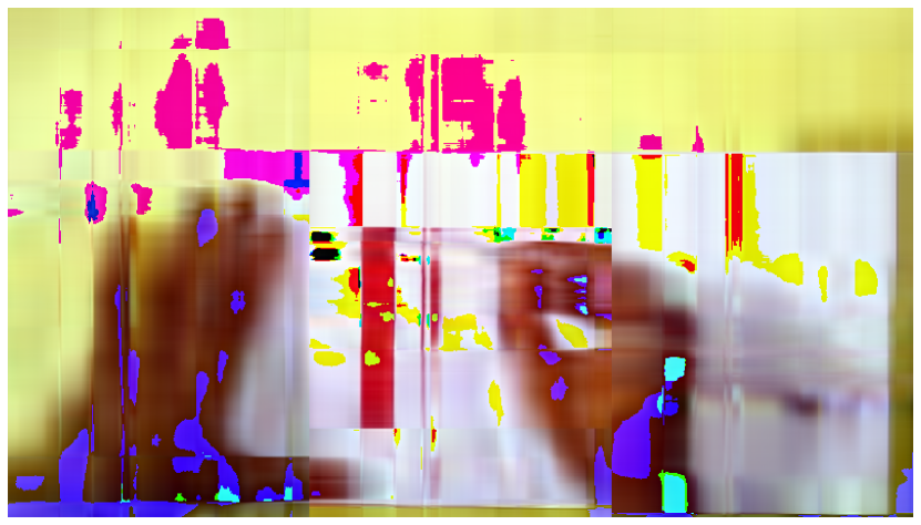
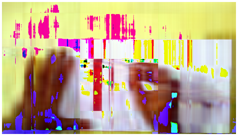
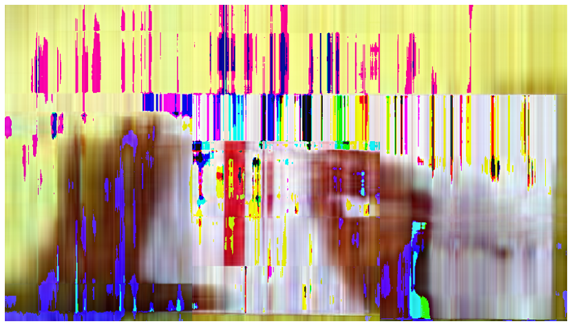
Similar improvement of the learned sketching matrices over the random sketching matrices can be observed when $k=10,m=10,20,30,40,\cdots,80$, see Figure 5.2. We also include the test error results in Table 5.2 for the case when $k=20,30$. Finally, in Figure 5.3, we visualize an example output of the algorithm for the case $k=10,m=20$ for the Logo dataset.

5.2 Comparing Random, Learned and Mixed

In Table 5.2, we investigate the performance of the mixed sketching matrices by comparing them with random and learned sketching matrices. In all scenarios, the mixed sketching matrices yield much better results than the random sketching matrices, and sometimes the results are comparable to those of learned sketching matrices. This means, in most cases it suffices to train half of the sketching matrix to obtain good empirical results, and at the same time, by our Theorem 4.1, we can use the remaining random half of the sketching matrix to obtain worst-case guarantees.

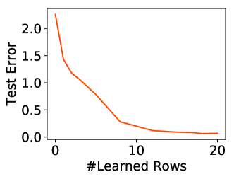
Moreover, if we do not fix the number of learned rows to be half, the test error increases as the number of learned rows decreases. In Figure 5.4, we plot the test error for the setting with $m=20,k=10$ using $100$ Logo matrices, running for $3000$ iterations.

Figure 5.4: Test errors of mixed sketching matrices with different number of “learned” rows.

5.3 Mixing Training Sets

In our previous experiments, we constructed a different learned sketching matrix $S$ for each data set. However, one can use a single random sketching matrix for all three data sets simultaneously. Next, we study the performance of a single learned sketching matrix for all three data sets. In Table 5.3, we constructed a single learned sketching matrix $S$ with $m=k=10$ on a training set containing $300$ matrices from Logo, Eagle and Friends (each has $100$ matrices). Then, we tested $S$ on Logo matrices and compared its performance to the performance of a learned sketching matrix $S_{L}$ trained on Logo dataset (i.e., using $100$ Logo matrices only), as well as to the performance of a random sketching $S_{R}$. The performance of the sketching matrix $S$ with a mixed training set from all three datasets is close to the performance of the sketching matrix $S_{L}$ with training set only from Logo dataset, and is much better than the performance of the random sketching matrix $S_{R}$.

Table 5.3: Evaluation of the sketching matrix trained on different sets

	Logo+Eagle+Friends	Logo only	Random
Test Error	0.67	0.27	5.19

5.4 Running Time

The runtimes of the algorithm with a random sketching matrix and our learned sketching matrix are the same, and are much less than the runtime of the “standard” SVD method (implemented in Pytorch). In Table 5.4, we present the runtimes of the algorithm with different types of sketching matrices (i.e., learned and random) on Logo matrices with $m=k=10$, as well as the training time of the learned case. Notice that training only needs to be done once, and can be done offline.

Table 5.4: Runtimes of the algorithm with different sketching matrices

SVD	Random	Learned-Inference	Learned-Training
2.2s	0.03s	0.03s	9481.25s

6 Conclusions

In this paper we introduced a learning-based approach to sketching algorithms for computing low-rank decompositions. Such algorithms proceed by computing a projection $SA$, where $A$ is the input matrix and $S$ is a random “sketching” matrix. We showed how to train $S$ using example matrices $A$ in order to improve the performance of the overall algorithm. Our experiments show that for several different types of datasets, a learned sketch can significantly reduce the approximation loss compared to a random matrix. Further, we showed that if we mix a random matrix and a learned matrix (by concatenation), the result still offers an improved performance while inheriting worst case guarantees of the random sketch component.

Appendix A The case of $m=1$

In this section, we denote the SVD of $A$ as $U^{A}\Sigma^{A}(V^{A})^{\top}$ such that both $U^{A}$ and $V^{A}$ have orthonormal columns and $\Sigma^{A}=\mathrm{diag}\{\lambda^{A}_{1},\cdots,\lambda^{A}_{d}\}$ is a diagonal matrix with nonnegative entries. For simplicity, we assume that for all $A\sim\mathcal{D}$, $1=\lambda_{1}\geq\cdots\geq\lambda_{d}$. We use $U_{i}^{A}$ to denote the $i$-th column of $U^{A}$, and similarly for $V_{i}^{A}$. Denote $\Sigma^{A}=\mathrm{diag}\{\lambda_{1}^{A},\cdots,\lambda_{d}^{A}\}$.

We want to find $[A]_{k}$, the rank-$k$ approximation of $A$. In general, it is hard to obtain a closed form expression of the output of Algorithm 1. However, for $m=1$, such expressions can be calculated. Indeed, if $m=1$, the sketching matrix becomes a vector $s\in\mathbb{R}^{1\times n}$. Therefore $[AV]_{k}$ has rank at most one, so it suffices to set $k=1$. Consider a matrix $A\sim\mathcal{D}$ as the input to Algorithm 1. By calculation, $SA=\sum_{i}\lambda_{i}^{A}\langle s,U_{i}^{A}\rangle(V_{i}^{A})^{\top}$, which is a vector. For example, if $S=U_{1}^{A}$, we obtain $\lambda_{1}^{A}(V_{1}^{A})^{\top}$. Note that in this section to emphasize that $m=1$ (i.e., $S$ is a vector), we denote $S$ as $s$. Since $SA$ is a vector, applying SVD on it is equivalent to performing normalization. Therefore,

$$V={\sum_{i=1}^{d}\lambda_{i}^{A}\langle s,U_{i}^{A}\rangle(V_{i}^{A})^{\top}\over\sqrt{\sum_{i=1}^{d}(\lambda_{i}^{A})^{2}\langle s,U_{i}^{A}\rangle^{2}}}$$

Ideally, we hope that $V$ is as close to $V_{1}^{A}$ as possible, because that means $[AV]_{1}V^{\top}$ is close to $\lambda_{1}^{A}U_{1}^{A}(V_{1}^{A})^{\top}$, which captures the top singular component of $A$, i.e., the optimal solution. More formally,

$$AV={\sum_{i=1}^{d}(\lambda^{A}_{i})^{2}\langle s,U^{A}_{i}\rangle U^{A}_{i}\over\sqrt{\sum_{i=1}^{d}(\lambda^{A}_{i})^{2}\langle s,U^{A}_{i}\rangle^{2}}}$$

We want to maximize its norm, which is:

$${\sum_{i=1}^{d}(\lambda^{A}_{i})^{4}\langle s,U^{A}_{i}\rangle^{2}\over\sum_{i=1}^{d}(\lambda^{A}_{i})^{2}\langle s,U_{i}^{A}\rangle^{2}}$$ (A.1)

We note that one can simplify (A.1) by considering only the contribution from the top left singular vector $U_{1}^{A}$, which corresponds to the maximization of the following expression:

$${\langle s,U_{1}^{A}\rangle^{2}\over\sum_{i=1}^{d}(\lambda^{A}_{i})^{2}\langle s,U^{A}_{i}\rangle^{2}}$$ (A.2)

Appendix B Optimization Bounds

Motivated by the empirical success of sketch optimization, we investigate the complexity of optimizing the loss function. We focus on the simple case where $m=1$ and therefore $S$ is just a (dense) vector. Our main observation is that a vector $s$ picked uniformly at random from the $d$-dimensional unit sphere achieves an approximately optimal solution, with the approximation factor depending on the maximum stable rank of matrices $A_{1},\cdots,A_{N}$. This algorithm is not particularly useful for our purpose, as our goal is to improve over the random choice of the sketching matrix $S$. Nevertheless, it demonstrates that an algorithm with a non-trivial approximation factor exists.

Definition B.1 (stable rank ($r^{\prime}$)).

For a matrix $A$, the stable rank of $A$ is defined as the squared ratio of Frobenius and operator norm of $A$. I.e.,

$$r^{\prime}(A)={||A||^{2}_{F}\over||A||^{2}_{2}}={\sum_{i}(\lambda^{A}_{i})^{2}\over\max_{i}(\lambda^{A}_{i})^{2}}.$$

Note that since we assume for all matrices $A\sim\mathcal{D}$, $1=\lambda^{A}_{1}\geq\cdots\geq\lambda_{d}^{A}>0$, for all these matrices $r^{\prime}(A)=\sum_{i}(\lambda^{A}_{i})^{2}$.

First, we consider the simplified objective function as in (A.2).

Lemma B.2.

A random vector $s$ which is picked uniformly at random from the $d$-dimensional unit sphere, is an $O(r^{\prime})$-approximation to the optimum value of the simplified objective function in Equation (A.2), where $r^{\prime}$ is the maximum stable rank of matrices $A_{1},\cdots,A_{N}$.

Proof:

We will show that

$$E\left[{\langle s,U_{1}^{A}\rangle^{2}\over\sum_{i=1}^{d}(\lambda^{A}_{i})^{2}\langle s,U^{A}_{i}\rangle^{2}}\right]=\Omega(1/r^{\prime}(A))$$

for all $A\sim\mathcal{D}$ where $s$ is a vector picked uniformly at random from $\mathbf{S}^{d-1}$. Since for all $A\sim\mathcal{D}$ we have ${\langle s,U_{1}^{A}\rangle^{2}\over\sum_{i=1}^{d}(\lambda^{A}_{i})^{2}\langle s,U^{A}_{i}\rangle^{2}}\leq 1$, by the linearity of expectation we have that the vector $s$ achieves an $O(r^{\prime})$-approximation to the maximum value of the objective function,

$$\sum_{j=1}^{N}{\langle s,U_{1}^{A_{j}}\rangle^{2}\over\sum_{i=1}^{d}(\lambda^{A_{j}}_{i})^{2}\langle s,U^{A_{j}}_{i}\rangle^{2}}.$$

First, recall that to sample $s$ uniformly at random from $\mathbf{S}^{d-1}$ we can generate $s$ as $\sum_{i=1}^{d}{\alpha_{i}U^{A}_{i}\over\sqrt{\sum_{i=1}^{d}\alpha_{i}^{2}}}$ where for all $i\leq d$, $\alpha_{i}\sim\mathcal{N}(0,1)$. This helps us evaluate $\mathbf{E}\left[{\langle s,U_{1}^{A}\rangle^{2}\over\sum_{i=1}^{d}(\lambda^{A}_{i})^{2}\langle s,U^{A}_{i}\rangle^{2}}\right]$ for an arbitrary matrix $A\sim\mathcal{D}$:

$$E =\mathbf{E}\left[{\langle s,U^{A}_{1}\rangle^{2}\over\sum_{i=1}^{d}(\lambda_{i}^{A})^{2}\langle s,U^{A}_{i}\rangle^{2}}\right]=\mathbf{E}\left[{(\alpha_{1})^{2}\over\sum_{i=1}^{d}(\lambda_{i}^{A}\cdot\alpha_{i})^{2}}\right]\geq\mathbf{E}\left[{(\alpha_{1})^{2}\over\sum_{i=1}^{d}(\lambda_{i}^{A}\cdot\alpha_{i})^{2}}|\Psi_{1}\cap\Psi_{2}\right]\cdot\Pr(\Psi_{1}\cap\Psi_{2})$$

where the events $\Psi_{1},\Psi_{2}$ are defined as:

$$\Psi_{1}\triangleq\mathbf{1}\left[|\alpha_{1}|\geq{1\over 2}\right],\text{and }\Psi_{2}\triangleq\mathbf{1}\left[\sum_{i=2}^{d}(\lambda_{i}^{A})^{2}(\alpha_{i})^{2}\leq 2\cdot r^{\prime}(A)\right]$$

Since $\alpha_{i}$s are independent, we have

$$E\geq\mathbf{E}\left[{(\alpha_{1})^{2}\over(\alpha_{1})^{2}+2\cdot r^{\prime}(A)}|\Psi_{1}\cap\Psi_{2}\right]\cdot\Pr(\Psi_{1})\cdot\Pr(\Psi_{2})\geq{1\over 8\cdot r^{\prime}(A)+1}\cdot\Pr(\Psi_{1})\cdot\Pr(\Psi_{2})$$

where we used that ${(\alpha_{1})^{2}\over(\alpha_{1})^{2}+2\cdot r^{\prime}(A)}$ is increasing for $(\alpha_{1})^{2}\geq{1\over 4}$. It remains to prove that $\Pr(\Psi_{1}),\Pr(\Psi_{2})=\Theta(1)$. We observe that, since $\alpha_{i}\sim\mathcal{N}(0,1)$, we have

$$\Pr(\Psi_{1}) =\Pr\left(|\alpha_{1}|\geq{1\over 2}\right)=\Theta(1)$$

Similarly, by Markov inequality, we have

$$\Pr(\Psi_{2})=\Pr\left(\sum_{i=1}^{d}(\lambda_{i}^{A})^{2}(\alpha_{i})^{2}\leq 2r^{\prime}(A)\right)\geq 1-\Pr\left(\sum_{i=1}^{d}(\lambda_{i}^{A})^{2}(\alpha_{i})^{2}>2r^{\prime}(A)\right)\geq{1\over 2}$$

$\square$

Next, we prove that a random vector $s\in\mathbf{S}^{d-1}$ achieves an $O(r^{\prime}(A))$-approximation to the optimum of the main objective function as in Equation (A.1).

Lemma B.3.

A random vector $s$ which is picked uniformly at random from the $d$-dimensional unit sphere, is an $O(r^{\prime})$-approximation to the optimum value of the objective function in Equation (A.1), where $r^{\prime}$ is the maximum stable rank of matrices $A_{1},\cdots,A_{N}$.

Proof:

We assume that the vector $s$ is generated via the same process as in the proof of Lemma B.2. It follows that

$$\mathbf{E}\left[{{\sum_{i=1}^{d}(\lambda^{A}_{i})^{4}\langle s,U^{A}_{i}\rangle^{2}\over\sum_{i=1}^{d}(\lambda^{A}_{i})^{2}\langle s,U^{A}_{i}\rangle^{2}}}\right]\geq\mathbf{E}\left[{(\alpha_{1})^{2}\over\sum_{i=1}^{d}(\lambda^{A}_{i})^{2}\cdot(\alpha_{i})^{2}}\right]=\Omega(1/r^{\prime}(A))$$

$\square$

Appendix C Generalization Bounds

Define the loss function as

$$\mathsf{L}(s)\triangleq-\mathbf{E}_{A\sim\mathcal{D}}\left[{\sum_{i=1}^{d}\left(\lambda^{A}_{i}\right)^{4}\langle s,U^{A}_{i}\rangle^{2}\over\sum_{i=1}^{d}\left(\lambda^{A}_{i}\right)^{2}\langle s,U^{A}_{i}\rangle^{2}}\right]$$

We want to find a vector $s\in\mathbf{S}^{d-1}$ to minimize $\mathsf{L}(s)$, where $\mathbf{S}^{d-1}$ is the $d$-dimensional unit sphere. Since $\mathcal{D}$ is unknown, we are optimizing the following empirical loss:

$$\hat{\mathsf{L}}_{\mathsf{Tr}}(s)\triangleq-\frac{1}{N}\sum_{j=1}^{N}\left[{\sum_{i=1}^{d}\left(\lambda^{A_{j}}_{i}\right)^{4}\langle s,U^{A_{j}}_{i}\rangle^{2}\over\sum_{i=1}^{d}\left(\lambda^{A_{j}}_{i}\right)^{2}\langle s,U^{A_{j}}_{i}\rangle^{2}}\right]$$

The importance of robust solutions

We start by observing that if $s$ minimizes the training loss $\hat{\mathsf{L}}$, it is not necessarily true that $s$ is the optimal solution for the population loss $\mathsf{L}$. For example, it could be the case that $\{A_{j}\}_{j=1,\cdots,N}$ are diagonal matrices with only $1$ non-zeros on the top row, while $s=(\epsilon,\sqrt{1-\epsilon^{2}},0,\cdots,0)$ for $\varepsilon$ close to $0$. In this case, we know that $\hat{\mathsf{L}}_{\mathsf{Tr}}(s)=-1$, which is at its minimum value.

However, such a solution is not robust. In the population distribution, if there exists a matrix $A$ such that $A=\mathrm{diag}(\sqrt{1-100\varepsilon^{2}},10\varepsilon,0,0,\cdots,0)$, insert $s$ into (A.1),

$${\sum_{i=1}^{d}\left(\lambda^{A}_{i}\right)^{4}\langle s,U^{A}_{i}\rangle^{2}\over\sum_{i=1}^{d}\left(\lambda^{A}_{i}\right)^{2}\langle s,U^{A}_{i}\rangle^{2}}={(1-100\varepsilon^{2})^{2}\varepsilon^{2}+10^{4}\varepsilon^{4}(1-\varepsilon^{2})\over(1-100\varepsilon^{2})\varepsilon^{2}+100\varepsilon^{2}(1-\varepsilon^{2})}<{\varepsilon^{2}+10^{4}\varepsilon^{4}\over 101\varepsilon^{2}-100\varepsilon^{4}}={1+10^{4}\varepsilon^{2}\over 101-100\varepsilon^{2}}$$

The upper bound is very close to $0$ if $\varepsilon$ is small enough. This is because when the denominator is extremely small, the whole expression is susceptible to minor perturbations on $A$. This is a typical example showing the importance of finding a robust solution. Because of this issue, we will show a generalization guarantee for a robust solution $s$.

Definition of robust solution

First, define event $\zeta_{A,\delta,s}\triangleq\mathbf{1}\left[\sum_{i=1}^{d}\left(\lambda^{A}_{i}\right)^{2}\langle s,U^{A}_{i}\rangle^{2}<\delta\right]$, which is the denominator in the loss function. Ideally, we want this event to happen with a small probability, which indicates that for most matrices, the denominator is large, therefore $s$ is robust in general. We have the following definition of robustness.

Definition C.1 (($\rho,\delta$)-robustness).

$s$ is ($\rho,\delta$)-robust with respect to $\mathcal{D}$ if $\mathbf{E}_{A\sim\mathcal{D}}[\zeta_{A,\delta,s}]\leq\rho$. $s$ is ($\rho,\delta$)-robust with respect to $\mathsf{Tr}$ if $\mathbf{E}_{A\sim\mathsf{Tr}}[\zeta_{A,\delta,s}]\leq\rho$.

For a given $\mathcal{D}$, we can define robust solution set that includes all robust vectors.

Definition C.2 (($\rho,\delta$)-robust set).

$\mathbf{M}_{\mathcal{D},\rho,\delta}$ is defined to be the set of all vectors $s\in\mathbf{S}^{d-1}$ s.t. $s$ is $(\rho,\delta$)-robust with respect to $\mathcal{D}$.

Estimating $\mathbf{M}_{\mathcal{D},\rho,\delta}$

The drawback of the above definition is that $\mathbf{M}_{\mathcal{D},\rho,\delta}$ is defined by the unknown distribution $\mathcal{D}$, so for fixed $\delta$ and $\rho$, we cannot tell whether $s$ is in $\mathbf{M}_{\mathcal{D},\rho,\delta}$ or not. However, we can estimate the robustness of $s$ using the training set. Specifically, we have the following lemma:

Lemma C.3 (Estimating robustness).

For a training set $\mathsf{Tr}$ of size $N$ sampled uniformly at random from $\mathcal{D}$, and a given $s\in\mathbb{R}^{d}$, a constant $1>\eta>0$, if $s$ is $(\rho,\delta)$-robust with respect to $\mathsf{Tr}$, then with probability at least $1-e^{-\frac{\eta^{2}pN}{2}}$, $s$ is $\left(\frac{\rho}{1-\eta},\delta\right)$-robust with respect to $\mathcal{D}$.

Proof:

Suppose that $\Pr_{A\sim\mathcal{D}}[\zeta_{A,\delta,s}]=\rho_{1}$, which means $\mathbf{E}\left[\sum_{A_{i}\in\mathsf{Tr}}\zeta_{A_{i},\delta,s}\right]=\rho_{1}N$. Since events $\zeta_{A_{i},\delta,s}$’s are $0$-$1$ random variables, by Chernoff bound,

$$\Pr\left(\sum_{A_{i}\in\mathsf{Tr}}\zeta_{A_{i},\delta,s}\leq(1-\eta)\rho_{1}N\right)\leq e^{-\frac{\eta^{2}\rho_{1}N}{2}}$$

If $\rho_{1}<\rho<\rho/(1-\eta)$, our claim is immediately true. Otherwise, we know $e^{-\frac{\eta^{2}\rho_{1}N}{2}}\leq e^{-\frac{\eta^{2}\rho N}{2}}$. Hence, with probability at least $1-e^{-\frac{\eta^{2}\rho N}{2}}$, $N\rho=\sum_{A_{i}\sim\mathsf{Tr}}\zeta_{A_{i},\delta,s}>(1-\eta)\rho_{1}N$. This implies that with probability at least $1-e^{-\frac{\eta^{2}\rho N}{2}}$, $\rho_{1}\leq\frac{\rho}{1-\eta}$. $\square$

Lemma C.3 implies that for a fixed solution $s$, if it is ($\rho,\delta$)-robust in $\mathsf{Tr}$, it is also $(O(\rho),\delta)$-robust in $\mathcal{D}$ with high probability. However, Lemma C.3 only works for a single solution $s$, but there are infinitely many potential $s$ on the $d$-dimensional unit sphere.

To remedy this problem, we discretize the unit sphere to bound the number of potential solutions. Classical results tell us that discretizing the unit sphere into a grid of edge length $\frac{\varepsilon}{\sqrt{d}}$ gives $\frac{C}{\varepsilon^{d}}$ points on the grid for some constant $C$ (e.g., see Section 3.3 in [Har-Peled et al., 2012] for more details). We will only consider these points as potential solutions, denoted as $\mathbf{\hat{B}}^{d}$. Thus, we can find a “robust” solution $s\in\mathbf{\hat{B}}^{d}$ with decent probability, using Lemma C.3 and union bound.

Lemma C.4 (Picking robust $s$).

For a fixed constant $\rho>0,1>\eta>0$, with probability at least $1-\frac{C}{\varepsilon^{d}}e^{-\frac{\eta^{2}\rho N}{2}}$, any $(\rho,\delta)$-robust $s\in\mathbf{\hat{B}}^{d}$ with respect to $\mathsf{Tr}$ is $\left(\frac{\rho}{1-\eta},\delta\right)$-robust with respect to $\mathcal{D}$.

Since we are working on the discretized solution, we need a new definition of robust set.

Definition C.5 (Discretized ($\rho,\delta$)-robust set).

$\mathbf{\hat{M}}_{\mathcal{D},\rho,\delta}$ is defined to be the set of all vector $s\in\mathbf{\hat{B}}^{d}$ s.t. $s$ is $(\rho,\delta$)-robust with respect to $\mathcal{D}$.

Using similar arguments as Lemma C.4, we know all solutions from $\mathbf{\hat{M}}_{\mathcal{D},\rho,\delta}$ are robust with respect to $\mathsf{Tr}$ as well.

Lemma C.6.

With probability at least $1-\frac{C}{\varepsilon^{d}}e^{-\frac{\eta^{2}\rho N}{3}}$, for a constant $\eta>0$, all solutions in $\mathbf{\hat{M}}_{\mathcal{D},\rho,\delta}$, are $((1+\eta)\rho,\delta)$-robust with respect to $\mathsf{Tr}$.

Proof:

Consider a fixed solution $s\in\mathbf{\hat{M}}_{\mathcal{D},\rho,\delta}$. Note that $\mathbf{E}\left[\sum_{A_{i}\in\mathsf{Tr}}\zeta_{A_{i},\delta,s}\right]=\rho N$ and $\zeta_{A_{i},\delta,s}$ are $0$-$1$ random variables. Therefore by Chernoff bound,

$$\Pr\left(\sum_{A_{i}\in\mathsf{Tr}}\zeta_{A_{i},\delta,s}\geq(1+\eta)\rho N\right)\leq e^{-\frac{\eta^{2}\rho N}{3}}.$$

Hence, with probability at least $1-e^{-\frac{\eta^{2}\rho N}{3}}$, $s$ is $((1+\eta)\rho,\delta)$-robust with respect to $\mathsf{Tr}$.

By union bound on all points in $\mathbf{\hat{M}}_{\mathcal{D},\rho,\delta}\subseteq\mathbf{\hat{B}}^{d}$, the proof is complete. $\square$

C.1 Generalization bound

Finally, we show the generalization bounds for robust solutions,. To this can we use Rademacher complexity to prove generalization bound. Define Rademacher complexity $R(\mathbf{\hat{M}}_{\mathcal{D},\rho,\delta}\circ\mathsf{Tr})$ as

$$R(\mathbf{\hat{M}}_{\mathcal{D},\rho,\delta}\circ\mathsf{Tr})\triangleq\frac{1}{N}\underset{\sigma\sim\{\pm 1\}^{N}}{\mathbf{E}}\sup_{s\in\mathbf{\hat{M}}_{\mathcal{D},\rho,\delta}}\sum_{j=1}^{N}\left[{\sigma_{j}\sum_{i=1}^{d}\left(\lambda^{A_{j}}_{i}\right)^{4}\langle s,U^{A_{j}}_{i}\rangle^{2}\over\sum_{i=1}^{d}\left(\lambda^{A_{j}}_{i}\right)^{2}\langle s,U^{A_{j}}_{i}\rangle^{2}}\right].$$

$R(\mathbf{\hat{M}}_{\mathcal{D},\rho,\delta}\circ\mathsf{Tr})$ is handy, because we have the following theorem (notice that the loss function takes value in $[-1,0]$):

Theorem C.7 (Theorem 26.5 in [Shalev-Shwartz and Ben-David, 2014]).

Given constant $\delta>0$, with probability of at least $1-\delta$, for all $s\in\mathbf{\hat{M}}_{\mathcal{D},\rho,\delta}$,

$$\mathsf{L}(s)-\hat{\mathsf{L}}_{\mathsf{Tr}}(s)\leq 2R(\mathbf{\hat{M}}_{\mathcal{D},\rho,\delta}\circ\mathsf{Tr})+4\sqrt{\frac{2\log(4/\delta)}{N}}$$

That means, it suffices to bound $R(\mathbf{\hat{M}}_{\mathcal{D},\rho,\delta}\circ\mathsf{Tr})$ to get the generalization bound. We have the following Lemma.

Lemma C.8 (Bound on $R(\mathbf{\hat{M}}_{\mathcal{D},\rho,\delta}\circ\mathsf{Tr})$).

For a constant $\eta>0$, with probability at least $1-\frac{C}{\varepsilon^{d}}e^{-\frac{\eta^{2}pN}{3}}$, $R(\mathbf{\hat{M}}_{\mathcal{D},\rho,\delta}\circ\mathsf{Tr})\leq(1+\eta)\rho+\frac{1-\delta}{2\delta}+\frac{d}{\sqrt{N}}$.

Proof:

Define $\rho^{\prime}=(1+\eta)\rho$. By Lemma C.6, we know that with probability $1-\frac{C}{\varepsilon^{d}}e^{-\frac{\eta^{2}pN}{3}}$, any $s\in\mathbf{\hat{M}}_{\mathcal{D},\rho,\delta}$ is ($\rho^{\prime},\delta$)-robust with respect to $\mathsf{Tr}$, hence $\sum_{A\in\mathsf{Tr}}\zeta_{A,\delta,s}\leq\rho^{\prime}N$. The analysis below is conditioned on this event.

Define $h_{A,\delta,s}\triangleq\max\{\delta,\sum_{i=1}^{d}(\lambda^{A}_{i})^{2}\langle s,U^{A}_{i}\rangle^{2}\}$. We know that with probability $1-\frac{C}{\varepsilon^{d}}e^{-\frac{\eta^{2}pN}{3}}$,

$$N\cdot R(\mathbf{\hat{M}}_{\mathcal{D},\rho,\delta}\circ\mathsf{Tr}) =\mathbf{E}_{\sigma\sim\{\pm 1\}^{N}}\sup_{s\in\mathbf{\hat{M}}_{\mathcal{D},\rho,\delta}}\sum_{j=1}^{N}{\sigma_{j}\sum_{i=1}^{d}\left(\lambda^{A_{j}}_{i}\right)^{4}\langle s,U^{A_{j}}_{i}\rangle^{2}\over\sum_{i=1}^{d}\left(\lambda^{A_{j}}_{i}\right)^{2}\langle s,U^{A_{j}}_{i}\rangle^{2}}$$

$$\leq\rho^{\prime}N+\mathbf{E}_{\sigma}\sup_{s\in\mathbf{\hat{M}}_{\mathcal{D},\rho,\delta}}\sum_{j=1}^{N}{\sigma_{j}\sum_{i=1}^{d}\left(\lambda^{A_{j}}_{i}\right)^{4}\langle s,U^{A_{j}}_{i}\rangle^{2}\over h_{A,\delta,s}}$$ (C.1)

where (C.1) holds because by definition, $h_{A,\delta,s}\geq\sum_{i=1}^{d}(\lambda^{A}_{i})^{2}\langle s,U^{A}_{i}\rangle^{2}$ if and only if $\zeta_{A,\delta,s}=1$, which happens for at most $\rho^{\prime}N$ matrices. Note that for any matrix $A_{j}$, ${\sigma_{j}\sum_{i=1}^{d}\left(\lambda^{A_{j}}_{i}\right)^{4}\langle s,U^{A_{j}}_{i}\rangle^{2}\over\sum_{i=1}^{d}\left(\lambda^{A_{j}}_{i}\right)^{2}\langle s,U^{A_{j}}_{i}\rangle^{2}}\leq 1$.

Now,

$$\mathbf{E}_{\sigma}\sup_{s\in\mathbf{\hat{M}}_{\mathcal{D},\rho,\delta}}\sum_{j=1}^{N}{\sigma_{j}\sum_{i=1}^{d}\left(\lambda^{A_{j}}_{i}\right)^{4}\langle s,U^{A_{j}}_{i}\rangle^{2}\over h_{A,\delta,s}}$$

$$\leq\quad \mathbf{E}_{\sigma}\sup_{s\in\mathbf{\hat{M}}_{\mathcal{D},\rho,\delta}}\sum_{j=1}^{N}\left({\mathbf{1}_{\sigma_{j}=1}\frac{\sum_{i=1}^{d}\left(\lambda^{A_{j}}_{i}\right)^{4}\langle s,U^{A_{j}}_{i}\rangle^{2}}{\delta}}-\mathbf{1}_{\sigma_{j}=-1}\sum_{i=1}^{d}\left(\lambda^{A_{j}}_{i}\right)^{4}\langle s,U^{A_{j}}_{i}\rangle^{2}\right)$$ (C.2)

$$=\quad \mathbf{E}_{\sigma}\sup_{s\in\mathbf{\hat{M}}_{\mathcal{D},\rho,\delta}}\sum_{j=1}^{N}\left({\sigma_{j}{\sum_{i=1}^{d}\left(\lambda^{A_{j}}_{i}\right)^{4}\langle s,U^{A_{j}}_{i}\rangle^{2}}}+{\mathbf{1}_{\sigma_{j}=1}{\sum_{i=1}^{d}\left(\lambda^{A_{j}}_{i}\right)^{4}\langle s,U^{A_{j}}_{i}\rangle^{2}}\left(\frac{1}{\delta}-1\right)}\right)$$

$$\leq\quad \frac{N}{2\delta}-\frac{N}{2}+\mathbf{E}_{\sigma}\sup_{s\in\mathbf{\hat{M}}_{\mathcal{D},\rho,\delta}}\sum_{j=1}^{N}{\sigma_{j}{\sum_{i=1}^{d}\left(\lambda^{A_{j}}_{i}\right)^{4}\langle s,U^{A_{j}}_{i}\rangle^{2}}}$$ (C.3)

The first inequality, (C.2), holds as ${\sum_{i=1}^{d}\left(\lambda^{A_{j}}_{i}\right)^{4}\langle s,U^{A_{j}}_{i}\rangle^{2}\over h_{A,\delta,s}}\in[\delta,1]$. It remains to bound the last term (C.3).

$$\mathbf{E}_{\sigma}\sup_{s\in\mathbf{\hat{M}}_{\mathcal{D},\rho,\delta}}\sum_{j=1}^{N}{\sigma_{j}{\sum_{i=1}^{d}\left(\lambda^{A_{j}}_{i}\right)^{4}\langle s,U^{A_{j}}_{i}\rangle^{2}}}\leq\sum_{i=1}^{d}\mathbf{E}_{\sigma}\sup_{s\in\mathbf{\hat{M}}_{\mathcal{D},\rho,\delta}}\sum_{j=1}^{N}{\sigma_{j}{\left\langle s,\left(\lambda^{A_{j}}_{i}\right)^{2}U^{A_{j}}_{i}\right\rangle^{2}}}$$ (C.4)

By contraction lemma of Rademacher complexity, we have

$$\mathbf{E}_{\sigma}\sup_{s\in\mathbf{\hat{M}}_{\mathcal{D},\rho,\delta}}\sum_{j=1}^{N}{\sigma_{j}{\left\langle s,\left(\lambda^{A_{j}}_{i}\right)^{2}U^{A_{j}}_{i}\right\rangle^{2}}} \leq\mathbf{E}_{\sigma}\sup_{s\in\mathbf{\hat{M}}_{\mathcal{D},\rho,\delta}}\sum_{j=1}^{N}{\sigma_{j}{\left\langle s,\left(\lambda^{A_{j}}_{i}\right)^{2}U^{A_{j}}_{i}\right\rangle}}$$

$$=\mathbf{E}_{\sigma}\sup_{s\in\mathbf{\hat{M}}_{\mathcal{D},\rho,\delta}}{{\left\langle s,\sum_{j=1}^{N}\sigma_{j}\left(\lambda^{A_{j}}_{i}\right)^{2}U^{A_{j}}_{i}\right\rangle}}$$

$$\leq\mathbf{E}_{\sigma}\left\|\sum_{j=1}^{N}\sigma_{j}\left(\lambda^{A_{j}}_{i}\right)^{2}U^{A_{j}}_{i}\right\|_{2}$$

Where the last inequality is by Cauchy-Schwartz inequality. Now, using Jensen’s inequality, we have

$$\mathbf{E}_{\sigma}\left\|\sum_{j=1}^{N}\sigma_{j}\left(\lambda^{A_{j}}_{i}\right)^{2}U^{A_{j}}_{i}\right\|_{2}\leq\left(\mathbf{E}_{\sigma}\left\|\sum_{j=1}^{N}\sigma_{j}\left(\lambda^{A_{j}}_{i}\right)^{2}U^{A_{j}}_{i}\right\|_{2}^{2}\right)^{1/2}=\left(\sum_{j=1}^{N}\left(\lambda^{A_{j}}_{i}\right)^{4}\right)^{1/2}\leq\sqrt{N}$$ (C.5)

Combining (C.1), (C.3), (C.4) and (C.5), we have $R(\mathbf{\hat{M}}_{\mathcal{D},\rho,\delta}\circ\mathsf{Tr})\leq\rho^{\prime}+\frac{1-\delta}{2\delta}+\frac{d}{\sqrt{N}}$. $\square$

Combining with Theorem C.7, we get our main theorem:

Theorem C.9 (Main Theorem).

Given a training set $\mathsf{Tr}=\{A_{j}\}_{j=1}^{N}$ sampled uniformly from $\mathcal{D}$, and fixed constants $1>\rho\geq 0,\delta>0,1>\eta>0$, if there exists a $(\rho,\delta)$-robust solution $s\in\mathbf{\hat{B}}^{d}$ with respect to $\mathsf{Tr}$, then with probability at least $1-\frac{C}{\varepsilon^{d}}e^{-\frac{\eta^{2}pN}{2}}-\frac{C}{\varepsilon^{d}}e^{-\frac{\eta^{2}pN}{3(1-\eta)}}$, for $s\in\mathbf{\hat{B}}^{d}$ that is a $(\rho,\delta)$-robust solution with respect to $\mathsf{Tr}$,

$$\mathsf{L}(s)\leq\hat{\mathsf{L}}_{\mathsf{Tr}}(s)+\frac{2(1+\eta)\rho}{1-\eta}+\frac{1-\delta}{\delta}+\frac{2d}{\sqrt{N}}+4\sqrt{\frac{2\log(4/\delta)}{N}}$$

Proof:

Since we can find $s\in\mathbf{\hat{B}}^{d}$ s.t. $s$ is $(\rho,\delta)$-robust with respect to $\mathsf{Tr}$, by Lemma C.4, with probability $1-\frac{C}{\varepsilon^{d}}e^{-\frac{\eta^{2}pN}{2}}$, $s$ is $(\frac{\rho}{1-\eta},\delta)$-robust with respect to $\mathcal{D}$. Therefore, $s\in\mathbf{\hat{M}}_{\mathcal{D},\frac{\rho}{1-\eta},\delta}$. Apply Lemma C.8, we have With probability at least $1-\frac{C}{\varepsilon^{d}}e^{-\frac{\eta^{2}\rho N}{3(1-\eta)}}$, $R(\mathbf{\hat{M}}_{\mathcal{D},\rho,\delta}\circ\mathsf{Tr})\leq\frac{\rho(1+\eta)}{1-\eta}+\frac{1-\delta}{2\delta}+\frac{d}{\sqrt{N}}$. Combined with Theorem C.7, the proof is complete. $\square$

In summary, Theorem C.9 states that if we can find a solution $s$ which “fits” the training set, and is very robust, then it generalizes to the test set.

Appendix D Missing Proofs of Section 4

Fact D.1 (Pythagorean Theorem).

If $A$ and $B$ are matrices with the same number of rows and columns, then $AB^{\top}=0$ implies $||A+B||_{F}^{2}=||A||_{F}^{2}+||B||_{F}^{2}$.

Proof: (Proof of Lemma 4.2)

Note that $AVV^{\top}$ is a row projection of $A$ on the $\mathrm{colsp}(V)$. Then, for any conforming $Y$,

$$(A-AVV^{\top})(AVV^{\top}-YV^{\top})^{\top} =A(I-VV^{\top})V(AV-Y)^{\top}=A(V-VV^{\top}V)(AV-Y)^{\top}=0.$$

where the last equality follows from the fact if $V$ has orthonormal columns then $VV^{\top}V=V$ (e.g., see Lemma 3.5 in [Clarkson and Woodruff, 2009]). Then, by the Pythagorean Theorem (Fact D.1), we have

$$||A-YV^{\top}||_{F}^{2}=||A-AVV^{\top}||_{F}^{2}+||AVV^{\top}-YV^{\top}||_{F}^{2}$$ (D.1)

Since $V$ has orthonormal columns, for any conforming $x$, $||x^{\top}V^{\top}||=||x||$. Thus, for any $Z$ of rank at most $k$,

$$||AVV^{\top}-[AV]_{k}V^{\top}||_{F}=||(AV-[AV]_{k})V^{\top}||_{F} =||AV-[AV]_{k}||_{F}$$

$$\leq||AV-Z||_{F}=||AVV^{\top}-ZV^{\top}||_{F}$$ (D.2)

Hence,

$$||A-[AV]_{k}V^{\top}||_{F}^{2} =||A-AVV^{\top}||_{F}^{2}+||AVV^{\top}-[AV]_{k}V^{\top}||_{F}^{2}\;\rhd\text{By \eqref{eq:pythagorean-rel}}$$

$$\leq||A-AVV^{\top}||_{F}^{2}+||AVV^{\top}-ZV^{\top}||_{F}^{2}\qquad\rhd\text{By \eqref{eq:second-term}}$$

This implies that $[AV]_{k}V^{\top}$ is a best rank-$k$ approximation of $A$ in the $\mathrm{colsp}(V)$. $\square$

References

- Allen-Zhu and Li (2016) Z. Allen-Zhu and Y. Li. Lazysvd: even faster svd decomposition yet without agonizing pain. In Advances in Neural Information Processing Systems, pages 974–982, 2016.
- Balcan et al. (2018) M.-F. Balcan, T. Dick, T. Sandholm, and E. Vitercik. Learning to branch. In International Conference on Machine Learning, pages 353–362, 2018.
- Baldassarre et al. (2016) L. Baldassarre, Y.-H. Li, J. Scarlett, B. Gözcü, I. Bogunovic, and V. Cevher. Learning-based compressive subsampling. IEEE Journal of Selected Topics in Signal Processing, 10(4):809–822, 2016.
- Bora et al. (2017) A. Bora, A. Jalal, E. Price, and A. G. Dimakis. Compressed sensing using generative models. In International Conference on Machine Learning, pages 537–546, 2017.
- Boutsidis and Gittens (2013) C. Boutsidis and A. Gittens. Improved matrix algorithms via the subsampled randomized hadamard transform. SIAM Journal on Matrix Analysis and Applications, 34(3):1301–1340, 2013.
- Candès et al. (2006) E. J. Candès, J. Romberg, and T. Tao. Robust uncertainty principles: Exact signal reconstruction from highly incomplete frequency information. IEEE Transactions on information theory, 52(2):489–509, 2006.
- Clarkson and Woodruff (2009) K. L. Clarkson and D. P. Woodruff. Numerical linear algebra in the streaming model. In Proceedings of the forty-first annual symposium on Theory of computing (STOC), pages 205–214, 2009.
- Clarkson and Woodruff (2017) K. L. Clarkson and D. P. Woodruff. Low-rank approximation and regression in input sparsity time. Journal of the ACM (JACM), 63(6):54, 2017.
- Cohen et al. (2015) M. B. Cohen, S. Elder, C. Musco, C. Musco, and M. Persu. Dimensionality reduction for k-means clustering and low rank approximation. In Proceedings of the forty-seventh annual ACM symposium on Theory of computing, pages 163–172, 2015.
- Davidov et al. (2004) D. Davidov, E. Gabrilovich, and S. Markovitch. Parameterized generation of labeled datasets for text categorization based on a hierarchical directory. In Proceedings of the 27th Annual International ACM SIGIR Conference on Research and Development in Information Retrieval, SIGIR ’04, pages 250–257, 2004.
- Donoho (2006) D. L. Donoho. Compressed sensing. IEEE Transactions on information theory, 52(4):1289–1306, 2006.
- Ghashami and Phillips (2014) M. Ghashami and J. M. Phillips. Relative errors for deterministic low-rank matrix approximations. In Proceedings of the twenty-fifth annual ACM-SIAM symposium on Discrete algorithms (SODA), pages 707–717, 2014.
- Ghashami et al. (2016) M. Ghashami, E. Liberty, J. M. Phillips, and D. P. Woodruff. Frequent directions: Simple and deterministic matrix sketching. SIAM Journal on Computing, 45(5):1762–1792, 2016.
- Gollapudi and Panigrahi (2019) S. Gollapudi and D. Panigrahi. Online algorithms for rent-or-buy with expert advice. In International Conference on Machine Learning, pages 2319–2327, 2019.
- Halko et al. (2011) N. Halko, P.-G. Martinsson, and J. A. Tropp. Finding structure with randomness: Probabilistic algorithms for constructing approximate matrix decompositions. SIAM review, 53(2):217–288, 2011.
- Hand and Voroninski (2018) P. Hand and V. Voroninski. Global guarantees for enforcing deep generative priors by empirical risk. In Conference On Learning Theory, 2018.
- Har-Peled et al. (2012) S. Har-Peled, P. Indyk, and R. Motwani. Approximate nearest neighbor: Towards removing the curse of dimensionality. Theory of computing, 8(1):321–350, 2012.
- Hsu et al. (2019) C.-Y. Hsu, P. Indyk, D. Katabi, and A. Vakilian. Learning-based frequency estimation algorithms. International Conference on Learning Representations, 2019.
- Imamoglu et al. (2018) N. Imamoglu, Y. Oishi, X. Zhang, G. Ding, Y. Fang, T. Kouyama, and R. Nakamura. Hyperspectral image dataset for benchmarking on salient object detection. In Tenth International Conference on Quality of Multimedia Experience, (QoMEX), pages 1–3, 2018.
- Khalil et al. (2017) E. Khalil, H. Dai, Y. Zhang, B. Dilkina, and L. Song. Learning combinatorial optimization algorithms over graphs. In Advances in Neural Information Processing Systems, pages 6348–6358, 2017.
- Khani et al. (2019) M. Khani, M. Alizadeh, J. Hoydis, and P. Fleming. Adaptive neural signal detection for massive MIMO. CoRR, abs/1906.04610, 2019.
- Kraska et al. (2018) T. Kraska, A. Beutel, E. H. Chi, J. Dean, and N. Polyzotis. The case for learned index structures. In Proceedings of the 2018 International Conference on Management of Data, pages 489–504, 2018.
- Liberty (2013) E. Liberty. Simple and deterministic matrix sketching. In Proceedings of the 19th ACM SIGKDD international conference on Knowledge discovery and data mining, pages 581–588, 2013.
- Lykouris and Vassilvitskii (2018) T. Lykouris and S. Vassilvitskii. Competitive caching with machine learned advice. In International Conference on Machine Learning, pages 3302–3311, 2018.
- Meng and Mahoney (2013) X. Meng and M. W. Mahoney. Low-distortion subspace embeddings in input-sparsity time and applications to robust linear regression. In Proceedings of the forty-fifth annual ACM symposium on Theory of computing, pages 91–100, 2013.
- Metzler et al. (2017) C. Metzler, A. Mousavi, and R. Baraniuk. Learned d-amp: Principled neural network based compressive image recovery. In Advances in Neural Information Processing Systems, pages 1772–1783, 2017.
- Mitzenmacher (2018) M. Mitzenmacher. A model for learned bloom filters and optimizing by sandwiching. In Advances in Neural Information Processing Systems, pages 464–473, 2018.
- Mousavi et al. (2015) A. Mousavi, A. B. Patel, and R. G. Baraniuk. A deep learning approach to structured signal recovery. In Communication, Control, and Computing (Allerton), 2015 53rd Annual Allerton Conference on, pages 1336–1343. IEEE, 2015.
- Nelson and Nguyên (2013) J. Nelson and H. L. Nguyên. Osnap: Faster numerical linear algebra algorithms via sparser subspace embeddings. In Foundations of Computer Science (FOCS), 2013 IEEE 54th Annual Symposium on, pages 117–126, 2013.
- Purohit et al. (2018) M. Purohit, Z. Svitkina, and R. Kumar. Improving online algorithms via ml predictions. In Advances in Neural Information Processing Systems, pages 9661–9670, 2018.
- Sarlos (2006) T. Sarlos. Improved approximation algorithms for large matrices via random projections. In 47th Annual IEEE Symposium on Foundations of Computer Science (FOCS), pages 143–152, 2006.
- Shalev-Shwartz and Ben-David (2014) S. Shalev-Shwartz and S. Ben-David. Understanding Machine Learning: From Theory to Algorithms. Cambridge University Press, 2014.
- Wang et al. (2016) J. Wang, W. Liu, S. Kumar, and S.-F. Chang. Learning to hash for indexing big data - a survey. Proceedings of the IEEE, 104(1):34–57, 2016.
- Woodruff (2014) D. P. Woodruff. Sketching as a tool for numerical linear algebra. Foundations and Trends® in Theoretical Computer Science, 10(1–2):1–157, 2014.
- Woolfe et al. (2008) F. Woolfe, E. Liberty, V. Rokhlin, and M. Tygert. A fast randomized algorithm for the approximation of matrices. Applied and Computational Harmonic Analysis, 25(3):335–366, 2008.
Appendix A The case of
In this section, we denote the SVD of as such that both and have orthonormal columns and is a diagonal matrix with nonnegative entries. For simplicity, we assume that for all , . We use to denote the -th column of , and similarly for . Denote .
We want to find , the rank- approximation of . In general, it is hard to obtain a closed form expression of the output of Algorithm 1. However, for , such expressions can be calculated. Indeed, if , the sketching matrix becomes a vector . Therefore has rank at most one, so it suffices to set . Consider a matrix as the input to Algorithm 1. By calculation, , which is a vector. For example, if , we obtain . Note that in this section to emphasize that (i.e., is a vector), we denote as . Since is a vector, applying SVD on it is equivalent to performing normalization. Therefore,
Ideally, we hope that is as close to as possible, because that means is close to , which captures the top singular component of , i.e., the optimal solution. More formally,