GetDist: a Python package for analysing Monte Carlo samples
Abstract
Monte Carlo techniques, including MCMC and other methods, are widely used and generate sets of samples from a parameter space of interest that can be used to infer or plot quantities of interest. This note outlines methods used the Python GetDist package to calculate marginalized one and two dimensional densities using Kernel Density Estimation (KDE). Many Monte Carlo methods produce correlated and/or weighted samples, for example produced by MCMC, nested, or importance sampling, and there can be hard boundary priors. GetDist’s baseline method consists of applying a linear boundary kernel, and then using multiplicative bias correction. The smoothing bandwidth is selected automatically following Botev et al. (2010), based on a mixture of heuristics and optimization results using the expected scaling with an effective number of samples (defined to account for MCMC correlations and weights). Two-dimensional KDE use an automatically-determined elliptical Gaussian kernel for correlated distributions. The package includes tools for producing a variety of publication-quality figures using a simple named-parameter interface, as well as a graphical user interface that can be used for interactive exploration. It can also calculate convergence diagnostics, produce tables of limits, and output in latex.
I Introduction
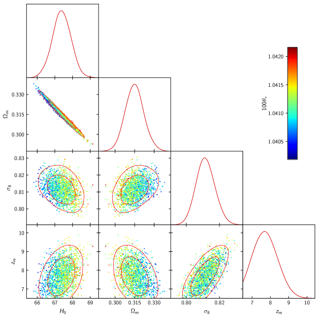
Monte Carlo (MC) sampling methods are widely used, from simulations to Markov Chain Monte Carlo (MCMC) sampling for Bayesian inference Metropolis et al. (1953); Hastings (1970); Neal (1993). Once samples have been generated, many (but not all) quantities of interest can easily be estimated from the samples, including parameter means, confidence limits and marginalized densities. GetDist is a Python package for computing these and making publication-quality figures111https://getdist.readthedocs.io/, install using pip install getdist. Source code at https://github.com/cmbant/getdist/ . An example is shown in Fig. 1, taken from the Planck satellite cosmological parameter analysis for which the package was originally developed Planck Collaboration VI (2018). The MC samples here are drawn from the posterior distribution of cosmological parameters using MCMC, and are shown (thinned) as coloured points in the figure. The full example parameter space is 27-dimensional, but since marginalization from samples simply corresponds to ignoring parameters, the marginalized 1D and 2D densities are just proportional to the local (weighted) sample density in the subspace of interest. The 1D curves show estimates of the marginalized density for some individual parameters, and the 2D contours show contours of equal marginalized probability that contain different fractions of the total probability. GetDist provides a simple Python and graphical interface for calculating the required densities and producing figures (using matplotlib Hunter (2007)); for many more examples see the plot gallery222https://getdist.readthedocs.io/en/latest/plot_gallery.html. This note is not intended to document the GetDist package (see the documentation), but to collect some notes and references for what the code is doing.
To calculate marginalized probabilities, or make 1D probability or confidence/exclusion plots we need a way to estimate the underlying marginalized probability density from the distribution of samples. This is easy to do approximately by just constructing histograms, however it may be unclear how wide to make the bins and the result is unlikely to be an accurate representation of the density. A Bayesian approach could attempt to solve for the distribution of the true density given the samples (and a model of how they were drawn), for example using a Gaussian process prior Prescott Adams et al. (2009); Adams et al. (2009); Donner and Opper (2018). While conceptually appealing and potentially very accurate, solutions typically involve a further step of MC sampling and can have non-trivial computational cost. There are also practical difficulties to making it very rigorous, for example one rarely has a good model for the exact sampling distributions of realistic MCMC chains. Instead we focus on fast and relatively simple conventional kernel density estimates, which effectively amount to using intelligently smoothed histograms with appropriately chosen smoothing widths. The main difficulties are how to choose the widths and how to handle hard boundary priors. In general the smoothing width could vary spatially, but for simplicity it is sufficient for many distributions of practical interest to use a fixed smoothing for each marginalized distribution as we assume. For MC samples, one option would be to generate so many samples that sampling noise is nearly negligible (so that a very narrow smoothing could be used), and this should of course be done when the sampling cost is low enough. However, using a good density estimate can dramatically reduce the number of samples that are required for a given target accuracy, potentially greatly reducing the computational cost of the MC needed to produce reliable results and nice figures.
GetDist can be used on independent single samples, but also has specific support for weighted samples and samples with substantial correlations as typically produced by MCMC algorithms. Weighted samples are the natural product of importance sampling, nested sampling Skilling (2004); Handley et al. (2015); Feroz and Hobson (2008), and various other sampling techniques. MCMC methods produce highly correlated samples, but once converged the chain of samples from standard Metropolis sampling and variants should be stationary. The MC sampling noise in general depends on both the correlations and the weights, so both need to be accounted for when estimating an appropriate kernel smoothing.
II Weighted samples
We present results for weighted samples for generality, so each sample in the parameter space of interest is associated with a weight (which can be unity for unweighted samples). Estimators for the mean of a function under the distribution are then given by weighted sums over sample points:
| (1) |
where . Define as the probability of getting sample point with weight , taking points to be independent for now. The expected value of the estimator of the mean is then
| (2) |
where here and below we neglect differences between and . The estimator will therefore be unbiased, , if
| (3) |
We shall assume weighted samples satisfy Eq. (3), which is true for importance weights where the weights are non-stochastic and given by for arbitrary constant . It also holds for MCMC chains where integer weights count the number of steps due to rejected proposals at each point so that , though in the case of MCMC the points are not independent (as discussed further below).
III Kernel Density Estimation (KDE)
Kernel Density Estimation (KDE) is the standard term for a wide class of non-parametric methods of estimating probability densities from samples, improving on simple histograms by making some weak assumptions about smoothness. There are many reviews of the basics (e.g. see Refs. Wand and Jones (1994a); Sheather (2004); Hansen (2009); Zambom and Dias (2012)). For analysis of MCMC samples, we can continue to run the MCMC until we have ‘enough’ samples; for good convergence using standard criteria, typically independent-equivalent samples (and even more KDE-equivalent samples, see Sect. III.4). This is rather larger than many cases where when KDE is applied to small samples of data, and as such more accurate methods that can be unstable with smaller numbers of samples can be used successfully. I’ll start by reviewing some of the basics, then discuss various complications due to boundaries and sample correlations, and then improved estimators using multiplicative bias correction.
The basic ingredient is an estimate of the form
| (4) |
where are the sampled points, with samples in total. This is sometimes called the “Parzen–Rosenblatt” window estimator. The kernel can be chosen in different ways; GetDist uses (slightly truncated) zero-centred Gaussians by default, with a width parameter (or more generally a covariance). The width parameter determines how broad the kernel is, and hence how smooth the estimated function is. In practice, assuming we are only interested in low-dimensional densities, to get good scaling with large number of samples, the samples can be binned (finely compared to the scale of ), to give sample counts in a set of bins with centres (with ). Also evaluating as a (finely) binned density we then have a simple convolution that is fast to evaluate using FFTs333Or directly if the number of points is relatively small. FFTs could also be replaced by fast gauss transforms (see e.g. http://www.umiacs.umd.edu/~morariu/figtree/):
| (5) |
In general we have weighted samples, with each sample having a weight each, in which case
| (6) |
where , and is now the weighted sum of the samples in each bin. In the continuum limit the histogram function is , and using Eq. (3) we have
where we drop the subscript on the expectations where confusion should not arise. The KDE estimator of Eq. (6) therefore has expectation
| (7) |
which converges to when tends to a delta function as the kernel width goes to zero ().
III.1 KDE bias and linear boundary kernels
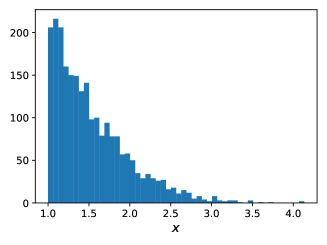
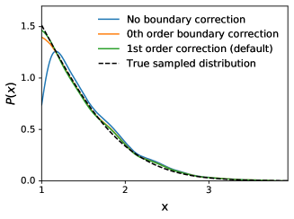
Where there is a boundary, for example a prior on some parameter that it is positive, smoothing over the boundary will give biased results, since there are no samples on one side (see Fig. 2). Let’s assume our function is of the form
| (8) |
where is zero in the disallowed region, and one in the allowed region444 can be more general. Specifically, for the binned densities it can account for the fraction of the bin allowed by the prior (e.g. for points where the prior cuts a bin in half). It could also account for other known locations of sharp features or structure Poluektov (2015) , and is a smooth function over the scale of the kernel (and equal to where ). Series expanding around using its assumed smoothness , from Eq. (6) in the continuum limit we have
| (9) | |||||
| (10) | |||||
| (11) |
where . Away from the boundary so that , we have and (for symmetric kernels), so the estimator is unbiased to linear order. The second order bias scales with the covariance of the kernel () and the local curvature of , and describes the broadening of peaks by convolution (hence typically overestimation of the variance). In units of the width of , the second order bias is , and hence is small as long as the kernel is narrow enough compared to .
With a boundary, the estimator is biased even at zeroth order. Normalizing by removes the leading bias, but leaves a linear bias if there is a non-zero gradient at the boundary (the convolution makes the shape at the boundary too flat). A simple solution to this is to use a linear boundary kernel Jones (1993): using a non-symmetric kernel near the boundary to remove the bias. Starting with a simple symmetric kernel , we can construct a more general kernel
| (12) |
and solve for coefficients to render the estimator unbiased. In one dimension this is straightforward to quadratic order555Giving a fourth order kernel, see e.g. Jones and Signorini (1997), but it gets messy in more dimensions, and the multiplicative correction (described in Sect. III.3) seems to be generally better at removing higher order biases. So here we restrict to linear kernels and set . We then have
| (13) | |||||
| (14) | |||||
| (15) |
Solving for unit response to and zero gradient bias then gives
| (16) |
where , , . The residual bias is then , even approaching the boundary. Note that the correction kernel is only different from the starting kernel within a kernel width of the boundary, since for symmetric kernels where . However, for generality the terms can also be calculated by full convolutions.
One issue with the linear boundary kernel estimators is that they are not guaranteed to be positive. A simple fix is to impose positivity by using the positive estimate
| (17) |
where is the simple de-biased kernel formed by normalizing by Jones and Foster (1996). We also always renormalize so that the kernel density integrates to unity (or has peak normalized to one for convenient plotting). If is only used as a pilot estimate for a later higher order estimator, accuracy of near the boundary is in any case not critical.
III.2 Statistical and total error
To quantify the error in the kernel estimator, people often use the mean integrated squared error
| (18) |
largely because it is convenient to calculate analytically in simple cases. There are contributions from bias and statistical noise. Assume for simplicity there are no boundary priors here, so Eq. (11) gives the leading bias
| (19) |
To see the dependence on the smoothing scale of the -dimensional kernel, we can define the kernel as , and hence
| (20) |
The bias is independent of whether the samples are weighted or correlated. The statistical term is more tricky however. For now, just take the sample locations to be independent. Then (taking to be non-stochastic)
| (21) | |||||
where . We can define an effective sample number
| (22) |
so that the leading statistical variance scales :
| (23) |
For small , the first term dominates.
The total mean integrated error of Eq. (18) is the sum of the bias and statistical terms, and evaluating the leading terms to get the asymptotic mean integrated squared error (AMISE) gives
| (24) |
Minimizing this with respect to gives , or explicitly an asymptotically-optimal kernel smoothing scale of
| (25) |
where .
Apart from the scaling with the effective number of samples , also scales with the curvature of via the dependence on : the larger the average squared second derivative, the more structure the gets smoothed out, and hence the smaller should be. But remember that this is specific to the simple linear kernel estimator of Eq. (4), assuming independent sample points.
III.3 Multiplicative bias correction
Using boundary kernels renders estimates that are unbiased to . However, there is still a systematic broadening of peaks, which can lead to systematically overestimated errors unless there are sufficiently many samples that . We can do better (or save computing time by generating fewer samples), by using a higher-order estimator.
Note that the simple estimator is exactly unbiased if the density is flat (or linear). We can therefore try to flatten the density before performing the convolutions. Specifically, doing the multiplicative bias correction to form
| (26) |
where is an approximation to the shape of , so that is nearly flat. Absent any prior information about the shape, the simplest thing to do is use , where is a standard linear kernel density estimate; the estimator then has bias away from boundaries (assuming sufficient smoothness of ) Jones et al. (1995). To improve the flattening near boundaries, we can take to be the linear boundary kernel estimate from the Sect. III.1. In principle the flattening can also be iterated, but for good choice of smoothing widths usually little is to be gained (and iterations will not converge due to random fluctuations being magnified). The simple multiplicative bias correction method compares well with other higher-order kernel methods for many distributions Jones and Signorini (1997) and seems to work well in practice as long as the density is indeed sufficiently smooth. In principle different bandwidths can be used for the pilot estimator and the final estimate (see e.g. Hengartnera and Matzner-Lober (2009) who recommend is over-smoothed compared to ), but for simplicity we take them to be the same. Other approaches to bias reduction are possible, including the ‘data sharpening’ Choi and Hall (1999); Hall and Minnotte (2002) method, which is a special case of a more general diffusion approach Botev et al. (2010).
Using multiplicative bias correction often generates nice smooth densities even with relatively small numbers of samples. However, note that this can make the sampling error on the result less immediately visually apparent when plotted than when using lower-order estimates that result in more obviously unsmooth densities. GetDist allows the multiplicative correction order to be changed as desired, but is set to first order by default (doing multiplicative bias correction once).
III.4 Correlated samples
In reality, samples from MCMC are correlated. Expressed in weighted form (where weights count the rejections of the next proposal), there are non-trivial weights and correlations between chain positions. Correlations will increase the error. However, perhaps surprisingly, correlations don’t have a dramatic effect on the optimal kernel bandwidth: the main impact of correlation on the variance does not scale with , since correlated errors between nearby cannot be lowered by more smoothing; see Refs. Hall et al. (1995); Sköld and Roberts (2003).
Eq. (24) for the error using independent weighted samples (equivalent to Ref. Sköld and Roberts (2003)) cannot be the full story when correlated samples are used with finite of practical interest. For example, proposals in orthogonal subdimensions could leave the parameter(s) of interest exactly unchanged between steps even though they appear as different points in the full-dimensional parameter space. This could be remedied by using a parameter-dependent in Eq.(24), where the weights now count all consecutive identical points in the parameter space of the kernel density. However, it is also clear that very small changes in a parameter, for example due to accepted proposals along very nearly orthogonal eigendirections, should contribute nearly the same as exactly identical points. In other words, whether or not the correlation matters when determining the bandwidth depends on the shape of the correlation function; e.g., whether there is high probability for , or whether the distribution is broad compared to .
In detail, we have
| (27) |
Assuming stationarity666Note that this is not valid for the output of nested sampling and other dynamic sampling methods; in these cases GetDist currently simply treats the samples as independent, which could be improved in future. leads to
| (28) |
and transforming then gives
| (29) |
This makes it clear that the result depends on the number of sequences of points within distance of each other, as determined by the local filter. Note that the last term in Eq. (29) contains a large contribution from points that have close to the same value (a fraction of the terms in the sum), even in the absence of correlations. If points separated by are strongly correlated with , the second term also has a contribution that is the same order as the first; this limit is what is considered in Ref. Sköld and Roberts (2003), and accounts for rejection steps that leave the parameter value exactly unchanged.777 Note that if the (integer) weights are from chain rejections during MCMC (but we neglect correlations between accepted points), then , where is the acceptance probability. Evaluating expectations gives (30) So for raw chains, neglecting correlations between accepted points, we have (31) This relates results in terms of weights to results in the literature terms of acceptance probability (e.g. Ref. Sköld and Roberts (2003)). In general we define an effective number of samples, dependent on which parameter subspace is included in the dimensions of , estimated from the samples, as888It is often a good approximation to estimate the 2D result from the separate 1D results; in GetDist there is an option whether to use the 2D expression or not (use_effective_samples_2D). Dependence of the optimal smoothing scale on is quite weak, so a ballpark number is sufficient in most cases. A more optimal bandwidth estimator would not use a single but account for anisotropy in the sampling statistics for sampling methods where different parameters are treated qualitatively differently or have different diffusion rates.
| (32) |
where the sum over can be taken only up to order of the correlation length () where the terms are significantly non-zero (and hence is reasonably fast to evaluate), and takes out the contribution expected for uncorrelated samples (estimated here roughly by a sum over widely separated small subset of samples). In the limit this definition therefore isolates the term that contributes to the total variance as
| (33) |
and hence includes the effect of exactly duplicated samples from MCMC rejection. The definition of Eq. (32) obeys consistency under sample-splitting, so it does not matter how samples are grouped up in to weighted samples or split up, and for uncorrelated samples reduces to Eq. (22). More generally, Eq. (32) very roughly includes other tight short-range correlation effects from MCMC sampling (but also some additional covariance that is actually mostly -independent, which ideally should not affect the bandwidth choice). As defined does however itself depend on . We take a fiducial value for estimating . Values of typically lie between and the defined in Eq. (49) below that determines the sampling errors on parameter means.
III.5 Choice of kernel bandwidth
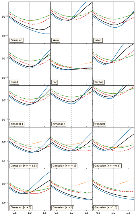
A good choice of kernel width is import to get good results: too broad, and features are washed out; too narrow, and sampling noise shows up. Recall from Eq. (24) that the Parzen–-Rosenblatt estimator has bias , and the statistical variance goes as . Minimizing with respect to gave (1D case of Eq. (25), corresponding to an overall convergence rate ). The constant in the optimal width depends on the distribution (and kernel); assuming one dimension and Gaussians gives the rule of thumb for parameter (‘normal scale rule’):
| (34) |
where is the standard deviation of the Gaussian smoothing Kernel to use and is an estimate of the standard deviation of parameter . In practice, for potentially non-Gaussian densities, can be set from a variety of scale measures, for example a width based on central quantiles to avoid over-estimation due to broad tails or a more refined method based on order statistics Janssen et al. (1995). However, simple scale rules can be quite suboptimal for many non-Gaussian densities. We only use a scale rule as a fallback when other methods fail and for choosing a fiducial scale for evaluating Eq. (32). To estimate we follow a simplified version of Ref. Janssen et al. (1995) (taking ], where is a the smallest parameter range enclosing of the probability ( for a unit Normal) and searching over ranges starting at ).
An optimal bandwidth choice can be derived using Eq. (25). The only problem here is that the optimal bandwidth depends on second derivatives () of the (unknown) density . Replacing the derivative term with an estimator gives so-called ’plug-in’ methods, which can perform much better especially for multi-modal distributions. For reviews and variations of methods see e.g. Jones et al. (1996); Eidous et al. (2010); Botev et al. (2010); Heidenreich et al. (2013). The main problem is that to estimate the second derivative you need to use a bandwidth, which gives you a recursive unknown bandwidth problem. Ref. Botev et al. (2010) present a neat solution, where the optimal bandwidth is obtained as an equation fixed point that can be found numerically called the “Improved Sheather-Jones” (ISJ) estimate. Using a Discrete Cosine Transform (DCT), this can also efficiently handle leading-order boundary effects, so that boundaries are not mistaken for large derivatives Botev et al. (2010). The method only requires one DCT of the binned data and some binned array dot products, and hence is fast; we adopt it as our auto-bandwidth selector999There can be multiple or no solutions to the fixed-point equation, esp. with some very flat bounded distributions. When multiple solution we take the larger one, and where no solutions we use the fallback of Eq. (34).. The DCT imposes even symmetry about boundaries, so we only use it for the bandwidth choice, not the actual KDE (the linear boundary kernel gives better accuracy by allowing general gradients at the boundaries).
With multiplicative bias correction the bias is higher order, with bias away from boundaries, so the total error scales as . Optimization now gives and overall convergence . Again the proportionality constant will depend on the distributions, various examples are given in Ref. Marzio and Taylor (2009). As a first guess we take the one-dimensional101010In general we can replace with for a higher order estimator where the leading bias goes as . rule of thumb
| (35) |
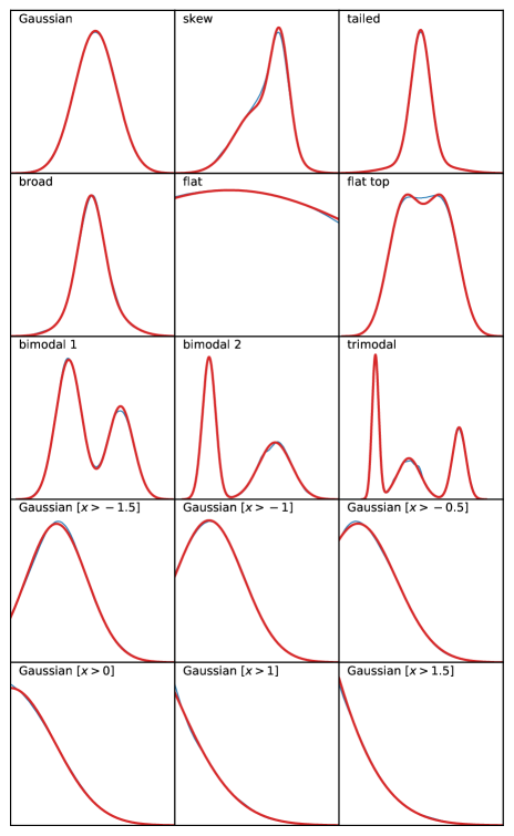
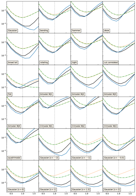
These smoothing widths are larger than for the basic Parzen–Rosenblatt estimator, and have lower statistical noise since the basic estimator is forced to have smaller widths to avoid significant bias. For , the smoothing width is about twice as broad as the basic estimator. A more refined estimate could be made analogously to the ISJ method using the asymptotic error for the higher order method, but we have not attempted to implement this. Eq. (35) is somewhat too small for normal distribution (which happens to give zero leading bias for this estimator Jones et al. (1995)), but somewhat too large for some truncated Gaussian shapes. See Fig. 3 for test results on various test distributions111111The code describing the exact distributions and for reproducing the figures is at https://github.com/cmbant/getdist/blob/master/getdist/tests/test_distributions.py,. Higher order bias correction can perform better, but starts to be more sensitive to having the bandwidth chosen optimally; as a default we use multiplicative boundary correction without iteration, which (in the test distributions) is almost always better than the Parzen estimator even when the auto-selected bandwidth is not optimal. In some cases using second order (once-iterated) multiplicative bias correction can give additional improvement. The GetDist package has settings options to tune exactly which method is use if required.
Multivariate bandwidth matrix
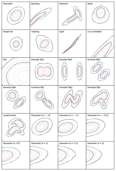
For two-dimensional densities we define the Kernel (following e.g. Ref. Wand and Jones (1993)) in terms of an isotropic Gaussian kernel and a kernel matrix , with , so that
| (36) |
If has identity covariance, , then is just the covariance of and hence
| (37) |
If we parameterize the Gaussian kernel covariance as , Eq. (37) becomes
| (38) |
where we defined as
| (39) |
assuming no boundary terms, where and and is even. For and both even, (and corresponding bandwidths) can be estimated following the fixed-point method121212When there is no solution for the fixed point, we instead use a plugin estimate for the bandwidth used for estimating . of Ref. Botev et al. (2010), where we assume an isotropic Gaussian kernel for evaluating . For the odd elements, the analogous argument to Ref. Botev et al. (2010) (Appendix E) using Eq. 3.2 from Wand and Jones (1994b) gives an equation for the bandwidth for estimating as
| (40) |
where
| (41) |
and can be estimated using the method for even elements.
In the case that the correlation is zero, Eq. (38) can be optimized analytically to give Wand and Jones (1994b)
| (42) |
In the general correlated case the minimum must be found numerically. In the specific case that the target distribution is Gaussian, the optimal Gaussian bandwidth matrix covariance is Wand and Jones (1993)
| (43) |
where is the sample covariance. This can be used to define a rule of thumb for Gaussian-like distributions, but in general (especially in the multi-modal case) can be very bad.
There are several other issues here
- •
-
•
With boundaries, the even derivative terms can be approximated by imposing reflection boundary conditions (i.e. evaluating using DCT), but with or odd, cannot be evaluated from the DCT transform (which assumes symmetry by construction). They can be evaluated by FFT if there are no sharp boundaries, but there is no easy way to approximately account for boundaries in this case.
-
•
Since the are evaluated using isotropic Gaussian kernels, they may be rather inaccurate if the optimal kernel is strongly elliptical.
We therefore adopt the following strategy:
-
•
Assuming there are no boundaries, or a boundary in only one of the or directions (but not both), use the sample covariance to perform a Cholesky parameter rotation to define uncorrelated transformed variables. The Cholesky rotation is chosen so that if or has a boundary it remains unchanged, so the boundary in the transformed parameters remains parallel to the edge of the DCT box. The transformed samples are scaled (so roughly isotropic) and binned, so that evaluation of using an isotropic kernel is not too suboptimal.
- •
- •
-
•
If there are boundaries in both the and directions, a Cholesky rotation cannot preserve both boundaries, so the samples are not transformed. The diagonal form of Eq. (42) is evaluated on the untransformed samples, unless the sample correlation is very high, in which case a Gaussian rule of thumb bandwidth is assumed using the sample covariance. When there are boundaries the fixed-point solution for the moment bandwidth can give solutions that are substantially too large, in which case we fall back to a rule of thumb for the moment bandwidth.
The expected asymptotic scaling of the optimal bandwidths are and respectively for methods with quadratic and quartic bias. With multiplicative bias correction we therefore scale the elements of the bandwidth matrix determined above to give
| (44) |
where the factor is empirically chosen. (In general we can replace with for a higher order estimator where the leading bias goes as ). See Fig. 3 for performance on typical distributions, showing that Eq. (44) slightly underestimates the bandwidth for a Gaussian distribution (and tail-truncated Gaussians), but is a reasonable compromise for most other cases and gives significant performance gains compared to the basic Parzen estimator.
IV Correlation lengths and sampling error on parameter means
From MCMC, possibly with post importance-sampling, the samples generally have non-trivial weights and non-trivial correlations. Consider a sample estimate for the mean of a parameter , given by
| (45) |
From independent unit-weight samples, the variance of the mean estimator is ; we can use this to define an effective for the correlated weighted samples. The variance of is given by
| (46) |
Defining , for chains in equilibrium we should have , where is the autocorrelation function at lag . Using this
| (47) |
If we assume that the correlation length is much shorter than the chain length131313Actually we don’t need to do this, the finite estimator for the autocorrelation from the samples follows the original expression., so for terms which matter, this is
| (48) |
We define this to be equal to so that
| (49) |
We can also define a correlation length by
| (50) |
so that . For unweighted samples corresponds to the standard definition of the correlation length. For importance sampled chains, it is the length in ‘weight units’ (it scales with the arbitrary normalization of the importance weights). We can also define a correlation length in ‘sample units’, so that , which gives an idea of how independent the different points are. In practice, to avoid sampling noise the upper limit for the sum is taken to be lag the lag at which the correlation has fallen to below some value (e.g. 0.05).
To estimate the error on Monte Carlo means, Eq. (49) can be estimated quickly using weighted sample convolutions and allows for both correlations and importance weights. In general there are correlations between parameters, so this is just an estimate for a single parameter, and will in general be optimistic (an upper limit).
V Discussion
Although GetDist 1.0 seems to work well for many simple cases, there are several assumptions and caveats. Future work could develop a kernel estimator optimized for other more-general non-stationary sampling distributions (e.g. the results of nested sampling). The boundary corrections as currently implemented require hard boundaries to be aligned with the parameter coordinates, which could be generalized to allow for an arbitrary prior mask; the leading-order correction would be a relatively straightforward extension, but optimization would require more work. The kernel optimization also currently does not account for the additional errors due to boundary correction, and may be suboptimal. More generally there may be non-trivial topology of the likelihood surface, for example highly multi-modal distributions with different characteristic scales on different modes. Although the basic methods described here will still work at some level, a global smoothing kernel is likely to be very suboptimal and there may be significant gains from implementing a more general method. The current implementation also only optimizes kernel widths for estimation of the density; for computation of integrals, such as tail confidence limits, this could be generalized. The code is open source on GitHub so contributions are welcome.
VI Acknowledgements
I thank Jesus Torrado for work on the Cobaya interface and him and other github users for contributions. I acknowledge support from the European Research Council under the European Union’s Seventh Framework Programme (FP/2007-2013) / ERC Grant Agreement No. [616170] and support by the UK STFC grant ST/P000525/1.
References
- Botev et al. (2010) Z. I. Botev, J. F. Grotowski, and D. P. Kroese, Ann. Statist. 38, 2916 (2010), eprint 1011.2602.
- Metropolis et al. (1953) N. Metropolis, A. W. Rosenbluth, M. N. Rosenbluth, A. H. Teller, and E. Teller, J. Chem. Phys. 21, 1087 (1953).
- Hastings (1970) W. Hastings, Biometrika 57, 97 (1970).
- Neal (1993) R. M. Neal (1993), http://cosmologist.info/Neal93.
- Planck Collaboration VI (2018) Planck Collaboration VI (Planck) (2018), eprint 1807.06209.
- Hunter (2007) J. D. Hunter, Computing in Science & Engineering 9, 90 (2007).
- Prescott Adams et al. (2009) R. Prescott Adams, I. Murray, and D. J. C. MacKay, arXiv e-prints (2009), eprint 0912.4896.
- Adams et al. (2009) R. P. Adams, I. Murray, and D. J. C. MacKay, in Advances in Neural Information Processing Systems 21, edited by D. Koller, D. Schuurmans, Y. Bengio, and L. Bottou (2009), pp. 9–16, https://papers.nips.cc/paper/3410-the-gaussian-process-density-sampler.pdf.
- Donner and Opper (2018) C. Donner and M. Opper, arXiv e-prints (2018), eprint 1805.11494.
- Skilling (2004) J. Skilling, in American Institute of Physics Conference Series, edited by R. Fischer, R. Preuss, and U. V. Toussaint (2004), pp. 395–405, URL http://www.inference.phy.cam.ac.uk/bayesys/.
- Handley et al. (2015) W. J. Handley, M. P. Hobson, and A. N. Lasenby, MNRAS 453, 4384 (2015), eprint 1506.00171, URL https://arxiv.org/abs/1506.00171.
- Feroz and Hobson (2008) F. Feroz and M. P. Hobson, Mon. Not. Roy. Astron. Soc. 384, 449 (2008), eprint 0704.3704.
- Lewis and Bridle (2002) A. Lewis and S. Bridle, Phys. Rev. D 66, 103511 (2002), eprint astro-ph/0205436.
- Neal (2005) R. M. Neal (2005), eprint math.ST/0502099.
- Lewis (2013) A. Lewis, Phys. Rev. D 87, 103529 (2013), eprint 1304.4473.
- Wand and Jones (1994a) M. Wand and M. Jones, Kernel Smoothing (Chapman and Hall, 1994a), ISBN 0412552701, http://cosmologist.info/ISBN/0412552701.
- Sheather (2004) S. J. Sheather, Statist. Sci. 19, 588 (2004), URL http://dx.doi.org/10.1214/088342304000000297.
- Hansen (2009) B. Hansen (2009), httt://www.ssc.wisc.edu/~bhansen/718/NonParametrics1.pdf.
- Zambom and Dias (2012) A. Z. Zambom and R. Dias, ArXiv e-prints (2012), eprint 1212.2812.
- Poluektov (2015) A. Poluektov, JINST 10, 02011 (2015), eprint 1411.5528.
- Jones (1993) M. Jones, Stat. & Comput. 3, 135 (1993), http://link.springer.com/content/pdf/10.1007/BF00147776.pdf.
- Jones and Signorini (1997) M. Jones and D. F. Signorini, J. Amer. Stat. Assoc. 92, 1063 (1997), http://www.jstor.org/stable/2965571.
- Jones and Foster (1996) M. Jones and P. J. Foster, Stat. Sinica 6, 1005 (1996), http://www3.stat.sinica.edu.tw/statistica/oldpdf/A6n414.pdf.
- Jones et al. (1995) M. Jones, O. Linton, and J. Nielsen, Biometrika 82, 327 (1995), http://www.jstor.org/stable/2337411.
- Hengartnera and Matzner-Lober (2009) N. W. Hengartnera and E. Matzner-Lober, ESAIM: Prob. & Stat. 13, 1 (2009), http://dx.doi.org/10.1051/ps:2007055.
- Choi and Hall (1999) E. Choi and P. Hall, Biometrika 86, 941 (1999), URL http://biomet.oxfordjournals.org/content/86/4/941.abstract.
- Hall and Minnotte (2002) P. Hall and M. C. Minnotte, J. Roy. Stat. Soc. Series B (Stat. Meth.) 64, 141 (2002), URL http://www.jstor.org/stable/3088854.
- Hall et al. (1995) P. Hall, S. N. Lahiri, and Y. K. Truong, Ann. Statist. 23, 2241 (1995), http://projecteuclid.org/euclid.aos/1034713655.
- Sköld and Roberts (2003) M. Sköld and G. Roberts, Scand. J. Stat. 30, 699 (2003), http://www.jstor.org/stable/4616797.
- Janssen et al. (1995) P. Janssen, J. S. Marron, N. Veraverbeke, and W. Sarle, J. Nonparam. Stat. 5, 359 (1995), http://dx.doi.org/10.1080/10485259508832654.
- Jones et al. (1996) M. Jones, J. Marron, and S. J. Sheather, J. Amer. Stat. Assoc. 91, 401 (1996), http://www.stat.washington.edu/courses/stat527/s14/readings/Jones_etal_JASA_1996.pdf.
- Eidous et al. (2010) O. M. Eidous, M. A. A. S. Marie, and M. H. Ebrahem, J. Mod. Appl. Stat. Meth. 9, 26 (2010), http://digitalcommons.wayne.edu/jmasm/vol9/iss1/26/.
- Heidenreich et al. (2013) N.-B. Heidenreich, A. Schindler, and S. Sperlich, AStA 97, 403 (2013), http://doi.org/10.1007/s10182-013-0216-y.
- Marzio and Taylor (2009) M. D. Marzio and C. C. Taylor, J. Nonparam. Stat. 21, 229 (2009), http://eprints.whiterose.ac.uk/42950/.
- Wand and Jones (1993) M. P. Wand and M. C. Jones, J. Amer. Stat. Assoc. 88, 520 (1993), http://www.jstor.org/stable/2290332.
- Wand and Jones (1994b) M. Wand and M. Jones, Comput. Stat. 9, 97 (1994b), URL ftp://math-libshare.math.ntu.edu.tw/131212-7377034.pdf.
- Duong and Hazelton (2003) T. Duong and M. Hazelton, J. Nonparam. Stat. 15, 17 (2003), URL http://www.mvstat.net/tduong/research/publications/duong-hazelton-2003-jns.pdf.