Model-Robust Inference for Clinical Trials that Improve Precision by Stratified Randomization and Covariate Adjustment

Abstract

Two commonly used methods for improving precision and power in clinical trials are stratified randomization and covariate adjustment. However, many trials do not fully capitalize on the combined precision gains from these two methods, which can lead to wasted resources in terms of sample size and trial duration. We derive consistency and asymptotic normality of model-robust estimators that combine these two methods, and show that these estimators can lead to substantial gains in precision and power. Our theorems cover a class of estimators that handle continuous, binary, and time-to-event outcomes; missing outcomes under the missing at random assumption are handled as well. For each estimator, we give a formula for a consistent variance estimator that is model-robust and that fully captures variance reductions from stratified randomization and covariate adjustment. Also, we give the first proof (to the best of our knowledge) of consistency and asymptotic normality of the Kaplan-Meier estimator under stratified randomization, and we derive its asymptotic variance. The above results also hold for the biased-coin covariate-adaptive design. We demonstrate our results using three completed, phase 3, randomized trial data sets of treatments for substance use disorder, where the variance reduction due to stratified randomization and covariate adjustment ranges from 1% to 36%.

Keywords: Covariate-adaptive randomization, generalized linear model, robustness.

1 Introduction

A joint guidance document from the U.S. Food and Drug Administration and the European Medicines Agency (FDA and EMA,, 1998) states that “Pretrial deliberations should identify those covariates and factors expected to have an important influence on the primary variable(s), and should consider how to account for these in the analysis to improve precision and to compensate for any lack of balance between treatment groups.” More recent regulatory guidance documents also encourage consideration of baseline variables in order to improve precision in randomized trials (EMA,, 2015; FDA,, 2019, 2020). Though there is a rich statistical literature on model-robust methods to adjust for baseline variables in randomized trials that use simple randomization, less is known for trials that use other forms of randomization. This is a practical concern since, as discussed below, many clinical trials use other forms of randomization.

“Covariate-adaptive randomization” refers to randomization procedures that take baseline variables into account when assigning participants to study arms. The goal is to achieve better balance across study arms in preselected strata of the baseline variables compared to simple randomization (which ignores baseline variables). E.g., balance on disease severity, a genetic marker, or another variable thought to be correlated with the primary outcome could be sought. The simplest and most commonly used type of covariate-adaptive randomization is stratified permuted block randomization (Zelen,, 1974), referred to as “stratified randomization” throughout, for conciseness.

Compared with simple randomization, covariate-adaptive randomization can be advantageous in minimizing imbalance and improving efficiency (Efron,, 1971; Pocock and Simon,, 1975; Wei,, 1978). Due to these benefits, covariate-adaptive randomization has become a popular approach in clinical trials. According to a survey by Lin et al., (2015), 183 out of their sample of 224 randomized clinical trials published in 2014 in leading medical journals used some form of covariate-adaptive randomization. Stratified randomization was implemented by 70% of trials in this survey. Another method for covariate-adaptive randomization is the biased-coin design by Efron, (1971), which we call “biased-coin randomization” throughout. Other examples include Wei’s urn design (Wei,, 1978) and rerandomization (Morgan and Rubin,, 2012). We only consider the following two types of covariate-adaptive randomization: stratified randomization and biased-coin randomization.

Concerns have been raised regarding how to perform valid statistical analyses at the end of trials that use covariate-adaptive randomization. Adjusting for stratification variables is recommended (Lachin et al.,, 1988; Kahan and Morris,, 2012; EMA,, 2015). However, this recommendation is not reliably carried out. Kahan and Morris, (2012) sampled 65 published trials from major medical journals from March to May 2010 and found that 41 implemented covariate-adaptive randomization (among which 29 used stratified randomization), but only 14 adjusted in the primary analysis for the variables used in the randomization procedure. Furthermore, many results on how to conduct the primary efficacy analysis in trials that use stratified randomization require one to assume a correctly specified regression model, e.g., Shao et al., (2010); Shao and Yu, (2013); Ma et al., (2015, 2018). Our focus is on model-robust estimators, i.e., estimators that do not require such an assumption when there is no missing data or when outcome data are missing completely at random; when censoring can depend on baseline variables, then additional assumptions are generally required.

Yang and Tsiatis, (2001) showed that the analysis of covariance (ANCOVA) estimator is consistent and asymptotically normal under simple randomization, and that this holds under arbitrary misspecification of the linear regression model used to construct the estimator. Analogous results for the ANCOVA estimator were shown by Bugni et al., (2018) under a variety of covariate-adaptive randomization procedures that include stratified and biased-coin randomization; however, their results only allow adjustment for the variables used in the randomization procedure. The proofs of our results build on key ideas from their work as described below. The results of Li and Ding, (2019) for the ANCOVA estimator are robust to arbitrary misspecification of the linear regression model; however, they use the randomization inference framework while many clinical trials are analyzed using the superpopulation inference framework (as done here); see Robins, (2002) for a comparison of these frameworks. All of the results in this paragraph are for the ANCOVA estimator, and so do not apply to logistic regression models for binary outcomes nor to commonly used models for time-to-event outcomes. Ye and Shao, (2019) derived asymptotic distributions for log-rank and score tests in survival analysis under covariate-adaptive randomization; however, estimation was not addressed.

For trials using stratified or biased-coin randomization, to the best of our knowledge, it was an open problem to determine (in the commonly used superpopulation inference framework and without making parametric model assumptions) the large sample properties of estimators that involve any of the following features: binary or time-to-event outcomes, adjustment for baseline variables in addition to those in the randomization procedure, and missing data under the missing at random assumption. This is the problem that we address, and we think that each of the above features can be important in the analysis of clinical trials. For example, binary and time-to-event outcomes are commonly used in clinical trials. According to a survey by Austin et al., (2010) on trials published in leading medical journals in 2007, 74 out of 114 trials involved binary or time-to-event outcomes. As we show in our data analyses, the addition of baseline variables beyond those used for stratified randomization can lead to substantial precision gains. Handling missing data is also important in order to avoid bias in treatment effect estimation.

Under regularity conditions, we prove that a large class of estimators is consistent and asymptotically normally distributed in randomized trials that use stratified or biased-coin randomization, and we give a formula for computing their asymptotic variance. This class of estimators consists of all M-estimators (van der Vaart,, 1998, p.41) that are consistent under simple randomization. It includes, e.g., the ANCOVA estimator for continuous outcomes; the standardized logistic regression estimator (Scharfstein et al.,, 1999; Moore and van der Laan, 2009a, ) for binary outcomes; the doubly-robust weighted least squares (DR-WLS) estimator from Marshall Joffe as described by Robins et al., (2007) for continuous and binary outcomes; and the Kaplan-Meier (K-M) estimator (Kaplan and Meier,, 1958) of survival functions and the augmented inverse probability weighted (AIPW) estimator of the restricted mean survival time (Díaz et al.,, 2019) for time-to-event outcomes.

Our theorems imply that under standard regularity conditions, whenever an estimator in our class is consistent and asymptotically normally distributed under simple randomization, then it is consistent and asymptotically normally distributed under stratified (or biased-coin) randomization with equal or smaller asymptotic variance. Also, its influence function is the same regardless of whether data is generated under simple, stratified or biased-coin randomization. This can be advantageous since for many estimators used to analyze randomized trials, their influence functions have already been derived under simple randomization. An estimator’s influence function can be input into our formula (5) to produce a consistent variance estimator under stratified and biased-coin randomization.

As in the aforementioned work, we assume that the randomization procedure and analysis method have been completely specified before the trial starts, as is typically required by regulators (FDA and EMA,, 1998; EMA,, 2015; FDA,, 2019, 2020).

In the next section, we describe three trial examples to which we apply our methods. In Section 3, we describe our setup, notation and assumptions. We present our main results in Section 4. In Section 5, we give example estimators for continuous and binary outcomes to which our general results apply. In Section 6, we present asymptotic results for the Kaplan-Meier estimator for time-to-event outcomes. Trial applications are provided in Section 7. Practical recommendations and future directions are discussed in Section 8.

2 Three completed trials that used stratified randomization

In some cases below, the outcomes in our analyses differ from the primary outcomes in the corresponding trials. This is because we wanted to use similar outcomes across trials for illustration. Our outcomes are all considered clinically important in the field of substance use disorder treatments.

2.1 Buprenorphine tapering and illicit opioid use (NIDA-CTN-0003)

The trial of “Buprenorphine tapering schedule and illicit opioid use” in the National Drug Abuse Treatment Clinical Trials Network (NIDA-CTN-0003), is a phase-3 randomized trial completed in 2005 (Ling et al.,, 2009). The goal was to compare the effects of a short or long taper schedule after buprenorphine stabilization of patients with opioid use disorder. Patients were randomized into two arms: 28-day taper (control, 259 patients, 36% missing outcomes) and 7-day taper (treatment, 252 patients, 21% missing outcomes), stratified by maintenance dose (3 levels) measured at randomization. The outcome of interest is a binary indicator of whether a participant’s urine tested at the end of the study is opioid-free. In addition to the stratification variable, we adjust for the following baseline variables: sex, opioid urine toxicology results, the Adjective Rating Scale for Withdrawal (ARSW), the Clinical Opiate Withdrawal Scale (COWS) and the Visual Analog Scale (VAS).

2.2 Prescription opioid addiction treatment (NIDA-CTN-0030)

The “Prescription Opioid Addiction Treatment Study” (NIDA-CTN-0030) is a phase-3 randomized trial completed in 2013 (Weiss et al.,, 2011). The goal was to determine whether adding individual drug counseling to the prescription of buprenorphine/naloxone would improve outcomes for patients with prescription opioid use disorder. Though this study adopted a 2-phase adaptive design, we focus on the first phase, in which patients were randomized into standard medical management (control, 330 patients, 10% missing outcomes) or standard medical management plus drug counseling (treatment, 335 patients, 13% missing outcomes). Randomization was stratified by the presence or absence of (i) a history of heroin use and (ii) current chronic pain, resulting in 4 strata. The outcome of interest is the proportion of negative urine laboratory results among all tests (treated as a continuous outcome between 0 and 1). Among all 5 urine laboratory tests during the first 4 weeks of phase I, if a patient missed two consecutive visits, then the outcome is regarded as missing. We included the following baseline variables in the analysis: randomization stratum, age, sex and urine laboratory results.

2.3 Internet-delivered treatment for substance abuse (NIDA-CTN-0044)

The phase-3 randomized trial “Internet-delivered treatment for substance abuse” (NIDA-CTN-0044) was completed in 2012 (Campbell et al.,, 2014). The goal was to evaluate the effectiveness of a web-delivered behavioral intervention, Therapeutic Education System (TES), in the treatment of substance abuse. Participants were randomly assigned to two arms: treatment as usual (control, 252 participants, 19% missing outcomes) and treatment as usual plus TES (treatment, 255 participants, 18% missing outcomes). Randomization was stratified by treatment site, patient’s primary substance of abuse (stimulant or non-stimulant) and abstinence status at baseline. Since the available data set for this trial did not include the treatment site variable, only the patient’s primary substance of abuse and abstinence status at baseline were included as strata (4 levels) in our analysis. After randomization, each participant was followed for 12 weeks with 2 urine laboratory tests per week. The outcome of interest is the proportion of negative urine lab results among all tests (treated as a continuous outcome between 0 and 1). If a participant missed visits of more than 6 weeks, the outcome is regarded as missing. We adjust for randomization stratum and the following additional baseline variables: age, sex and urine laboratory result.

We also analyze a second outcome: time to abstinence, defined as the time to first two consecutive negative urine tests during the study. Censoring time is defined as the first missing visit. We used the data from the first 6 weeks of follow-up in our data analysis of this time-to-event outcome, during which 99% of the events occurred.

3 Definitions and assumptions

3.1 Data generating distributions

We focus on two-arm randomized trials that use simple, stratified or biased-coin randomization. Let $n$ denote the sample size. For each participant $i=1,\dots,n$, let $Y_{i}$ denote the primary outcome, $M_{i}$ denote whether $Y_{i}$ is non-missing ($M_{i}=1$) or missing ($M_{i}=0$), $A_{i}$ denote study arm assignment ($A_{i}=1$ if assigned to treatment and $A_{i}=0$ if assigned to control), and $\boldsymbol{X}_{i}$ denote a vector of baseline covariates. This notation is for real-valued outcomes, e.g. continuous or binary outcomes. Modified definitions, assumptions, and results for time-to-event outcomes are in Section 6.

We use the Neyman-Rubin potential outcomes framework (Neyman et al.,, 1990), which assumes the existence of potential outcomes $Y_{i}(0)$ and $Y_{i}(1)$ for each participant $i$. These represent the outcome that would be observed under assignment to study arm $0$ or $1$, respectively. Though using potential outcomes introduces additional notation, it is needed in order to rigorously define the data generating distributions under the different randomization procedures that we consider. We make the following consistency assumption linking the observed outcome $Y_{i}$ to the potential outcomes: $Y_{i}=Y_{i}(A_{i})=Y_{i}(1)A_{i}+Y_{i}(0)(1-A_{i})$ for each participant $i$. Also, let $M_{i}(a)$ be the indicator of whether participant $i$ would have a non-missing outcome if they get assigned to study arm $a\in\{0,1\}$. We assume, analogous to the consistency assumption above, that $M_{i}=M_{i}(A_{i})=M_{i}(1)A_{i}+M_{i}(0)(1-A_{i})$.

For each participant $i$, we define the full data vector (including potential outcomes, some of which are not observed) $\boldsymbol{W}_{i}=(Y_{i}(1),Y_{i}(0),M_{i}(1),M_{i}(0),\boldsymbol{X}_{i})$ and the observed data vector $\mathbf{O}_{i}=(A_{i},\boldsymbol{X}_{i},Y_{i}M_{i},M_{i})$. The reason that the product $Y_{i}M_{i}$ appears in the observed data vector $\mathbf{O}_{i}$ is to encode that whenever the outcome is missing ($M_{i}=0$), the outcome value $Y_{i}$ is not available in $\mathbf{O}_{i}$ (since $Y_{i}M_{i}=0$). The data available to the analyst at the end of the trial are $\mathbf{O}_{1},\dots,\mathbf{O}_{n}$.

We make the following assumptions on the distribution of $\{\boldsymbol{W}_{1},\dots,\boldsymbol{W}_{n}\}$:

Assumption 1.

1. $\boldsymbol{W}_{i},i=1,\dots,n$ are independent, identically distributed samples from an unknown joint distribution $P$ on $\boldsymbol{W}=(Y(1),Y(0),M(1),M(0),\boldsymbol{X})$.

2. Missing at random: $M(a)\mbox{$\perp\!\!\!\perp$}Y(a)|\boldsymbol{X}$ for each arm $a\in\{0,1\}$, where $\perp\!\!\!\perp$ denotes independence.

Throughout, we use $E$ to denote the expectation with respect to distribution $P$.

3.2 Randomization procedures: simple, stratified, and biased-coin

First consider simple randomization, which assigns study arms $A_{1},\dots,A_{n}$ by independent Bernoulli draws each with fixed probability $\pi$ of being 1, e.g., using a random number generator. By design, the draws are independent of each other and of all participant characteristics measured before randomization or not impacted by randomization. Therefore, we have that $(A_{1},\dots,A_{n})$ is independent of $(\boldsymbol{W}_{1},\dots,\boldsymbol{W}_{n})$, and that the observed data $\mathbf{O}_{1},\dots,\mathbf{O}_{n}$ are independent, identically distributed.

Next consider stratified or biased-coin randomization, where treatment allocation depends on predefined baseline strata, such as gender, age, site, disease severity, or combinations of these. We refer to the baseline strata that are used in the randomization procedure as “randomization strata”. The baseline stratum of participant $i$ is denoted by the single, categorical variable $S_{i}$ taking $K$ possible values. For example, if randomization strata are defined by 4 sites and a binary indicator of high disease severity, then $S$ has $K=8$ possible values. Let $S_{i}$ denote the stratification variable for participant $i$ and let $\mathcal{S}=\{1,\dots,K\}$ denote the set of all $K$ randomization strata. The goal of stratified or biased-coin randomization is to achieve balance in each stratum; that is, the proportion of participants assigned to the treatment arm is targeted to the prespecified proportion $\pi\in(0,1)$, e.g. $\pi=0.5$. Throughout, the stratification variable $S$ is encoded in the baseline covariate vector $\boldsymbol{X}$ using $K-1$ dummy variables that make up the first $K-1$ components of $\boldsymbol{X}$ (which can include additional baseline variables).

Stratified randomization uses permuted blocks to assign treatment. For each randomization stratum, a randomly permuted block with fraction $\pi$ 1’s (representing treatment) and $(1-\pi)$ 0’s (representing control) is used for sequential allocation. When a block is exhausted, a new block is used.

Biased-coin randomization can be applied when $\pi=0.5$ and it allocates participants sequentially by the following rule for $k=1,\dots,n$:

$$P(A_{k}=1|S_{1},\dots,S_{k},A_{1},\dots,A_{k-1})=\left\{\begin{array}[]{rc}0.5,&\mbox{ if }\sum_{i=1}^{k-1}(A_{i}-0.5)I\{S_{i}=S_{k}\}=0\\ \lambda,&\mbox{ if }\sum_{i=1}^{k-1}(A_{i}-0.5)I\{S_{i}=S_{k}\}<0\\ 1-\lambda,&\mbox{ if }\sum_{i=1}^{k-1}(A_{i}-0.5)I\{S_{i}=S_{k}\}>0\end{array}\right.$$

where $\lambda\in(0.5,1]$, $I\{Z\}$ is the indicator function that has value $1$ if $Z$ is true and $0$ otherwise, and by convention the first participant is assigned with probability $0.5$ to each arm. Our results for biased-coin randomization assume that $\pi=0.5$.

When comparing the three types of randomization procedures (simple, stratified, or biased-coin), we assume that all use the same value of $\pi$. For the stratified randomization and biased-coin designs, it follows by construction (and was shown by Bugni et al.,, 2018) that the study arm assignments $(A_{1},\dots,A_{n})$ are conditionally independent of the participant baseline variables and potential outcomes $(\boldsymbol{W}_{1},\dots,\boldsymbol{W}_{n})$ given the randomization strata $(S_{1},\dots,S_{n})$. Intuitively, this is because the study arm assignment procedure only has access to the participants’ randomization strata (and nothing else about the participants). Under stratified or biased-coin randomization, the observed data vectors $\mathbf{O}_{1},\dots,\mathbf{O}_{n}$ are not independent.

Under any of the three randomization procedures, the observed data vectors $\mathbf{O}_{1},\dots,\mathbf{O}_{n}$ are identically distributed; that is, the distribution of $\mathbf{O}_{1}$ is the same as that of $\mathbf{O}_{2}$, etc. Let $P^{*}$ denote this distribution, i.e., the distribution of a generic, observed data vector $\mathbf{O}=(A,\boldsymbol{X},YM,M)$. This distribution is the same for each of the three randomization procedures, and is that induced by first drawing a single realization $\boldsymbol{W}=(Y(1),Y(0),M(1),M(0),\boldsymbol{X})$ from the distribution $P$ (see Assumption 1), then drawing $A$ as an independent Bernoulli draw with probability $\pi$ of being $1$, and lastly applying the consistency assumptions $Y=Y(1)A+Y(0)(1-A)$ and $M=M(1)A+M(0)(1-A)$ to construct $Y$, the (non)-missingness indicator $M$, and their product $YM$. The corresponding expectation with respect to $P^{*}$ is denoted $E^{*}$, which is used below. The claims in this paragraph are proved in the Supplementary Material.

3.3 Targets of Inference (Estimands) and Estimators

For continuous and binary outcomes, our goal is to estimate a population parameter ${\Delta}^{*}$, which is a contrast between the marginal distributions of $Y(1)$ and $Y(0)$. For example, the parameter of interest can be the population average treatment effect, defined as $\Delta^{*}=E[Y(1)]-E[Y(0)]$.

We consider M-estimators of $\Delta^{*}$ (van der Vaart,, 1998, Ch. 5). Let $\boldsymbol{\theta}=(\Delta,\boldsymbol{\beta}^{t})^{t}$ denote a column vector of $p+1$ parameters where $\Delta\in\mathbb{R}$ is the parameter of interest and $\boldsymbol{\beta}\in\mathbb{R}^{p}$ is a column vector of $p$ nuisance parameters. We define the M-estimator $\widehat{\boldsymbol{\theta}}=(\widehat{\Delta},\widehat{\boldsymbol{\beta}}^{t})^{t}$ to be the solution to the following estimating equations:

$$\sum_{i=1}^{n}\boldsymbol{\psi}(A_{i},\boldsymbol{X}_{i},Y_{i},M_{i};\boldsymbol{\theta})=\boldsymbol{0},$$ (1)

where $\boldsymbol{\psi}$ is a column vector (with $p+1$ components) of known functions. We define $\widehat{\Delta}$ to be the estimator of $\Delta^{*}$. We assume that $\boldsymbol{\psi}(A,\boldsymbol{X},Y,M;\boldsymbol{\theta})$ does not depend on the outcome $Y$ when $M=0$ (since $Y$ is missing in this case). Many estimators used in clinical trials, including all estimators defined in Section 5.1, can be expressed as solutions to estimating equations (1) for an appropriately chosen estimating function $\boldsymbol{\psi}$.

For time-to-event outcomes, the K-M estimator of the survival curve is commonly used. Since it is not an M-estimator, our general result (Theorem 1) for M-estimators below does not apply. We separately prove analogous results for the K-M estimator as described in Section 6.

We assume regularity conditions similar to the classical conditions that are used for proving consistency and asymptotic linearity of M-estimators for independent, identically distributed data, as given in Section 5.3 of van der Vaart, (1998). One of the conditions is that the expectation of the estimating equations

$$E^{*}[\boldsymbol{\psi}(A,\boldsymbol{X},Y,M;\boldsymbol{\theta})]=\boldsymbol{0},$$ (2)

has a unique solution in $\theta$, which is denoted as $\underline{\boldsymbol{\theta}}=(\underline{\Delta},\underline{\boldsymbol{\beta}}^{t})^{t}$. The other regularity conditions are given in the Supplementary Material.

We assume that the estimating equations $\boldsymbol{\psi}$ were chosen to ensure that the property $\Delta^{*}=\underline{\Delta}$ holds. This property is generally needed to show consistency of the M-estimator $\widehat{\Delta}$ for $\Delta^{*}$ under simple randomization, and has previously been proved for all of the estimators in Section 5.1. In general, whether the property $\Delta^{*}=\underline{\Delta}$ holds does not depend on the randomization procedure (simple, stratified, or biased-coin randomization); this is because the property depends only on $\boldsymbol{\psi}$, $P$ and $P^{*}$.

Results in Section 5.3 of van der Vaart, (1998) imply that under simple randomization, given Assumption 1 and the regularity conditions in the Supplementary Material, $\widehat{\Delta}$ converges in probability to $\underline{\Delta}$ and is asymptotically normally distributed with asymptotic variance that we denote by $\widetilde{V}$. We focus on determining what happens under stratified or biased-coin randomization, where our main result (Section 4) is that consistency and asymptotic normality still hold but the asymptotic variance may be smaller (and a consistent variance estimator is given).

4 Main result

Consider the setup in Section 3.3, where the M-estimator $\widehat{\Delta}$ is defined. We prove the following theorem:

Theorem 1.

Assume the regularity conditions in the Supplementary Material, $\Delta^{*}=\underline{\Delta}$, and Assumption 1. Under simple, stratified, or biased-coin randomization, we have consistency ($\widehat{\Delta}\rightarrow\Delta^{*}$ in probability) and

$$\sqrt{n}(\widehat{\Delta}-\Delta^{*})=\frac{1}{\sqrt{n}}\sum_{i=1}^{n}IF(A_{i},\boldsymbol{X}_{i},Y_{i},M_{i})+o_{p}(1),$$ (3)

where the influence function $IF(A,\boldsymbol{X},Y,M)$ is the first entry of $-\boldsymbol{B}^{-1}\boldsymbol{\psi}(A,\boldsymbol{X},Y,M;\underline{\boldsymbol{\theta}})$ for $\boldsymbol{B}=E^{*}\left[\frac{\partial}{\partial\boldsymbol{\theta}}\boldsymbol{\psi}(A,\boldsymbol{X},Y,M;\boldsymbol{\theta})\Big{|}_{\boldsymbol{\theta}=\underline{\boldsymbol{\theta}}}\right]$.

For stratified and biased-coin randomization, $\sqrt{n}(\widehat{\Delta}-\Delta^{*})\xrightarrow{d}N(0,V)$ for

$$V=\widetilde{V}-\frac{1}{\pi(1-\pi)}E^{*}\left[E^{*}\left\{(A-\pi)IF(A,\boldsymbol{X},Y,M)|S\right\}^{2}\right],$$ (4)

where $\widetilde{V}=E^{*}\{IF(A,\boldsymbol{X},Y,M)^{2}\}$ is the asymptotic variance under simple randomization. The asymptotic variance $V$ can be consistently estimated by formula (5) below.

Theorem 1 implies that given our setup and assumptions, whenever an M-estimator $\widehat{\Delta}$ is consistent and asymptotically normally distributed under simple randomization, then it is consistent and asymptotically normally distributed under stratified (or biased-coin) randomization with equal or smaller asymptotic variance. Also, its influence function is the same regardless of whether data is generated under simple, stratified, or biased-coin randomization; this can be advantageous since for many estimators used to analyze randomized trials, their influence functions have already been derived under simple randomization. The last display in Theorem 1 gives a simple formula for calculating the asymptotic variances for these estimators under the other two randomization procedures, in terms of the influence function.

For the unadjusted estimator $\widehat{\Delta}=\sum_{i=1}^{n}Y_{i}A_{i}/\sum_{i=1}^{n}A_{i}-\sum_{i=1}^{n}Y_{i}(1-A_{i})/\sum_{i=1}^{n}(1-A_{i})$, our Theorem 1 is equivalent to Theorem 4.1 of Bugni et al., (2018) under stratified or biased-coin randomization. In the special case of continuous outcomes, if the ANCOVA estimator is used with $X=S$, then Theorem 1 is equivalent to the result in section 4.2 of Bugni et al., (2018) under stratified or biased-coin randomization, though their results also handle other types of covariate-adaptive randomization.

Theorem 1 above extends the results of Bugni et al., (2018) to handle the class of M-estimators, that is, estimators calculated by solving estimating equations (1). This includes, for example, the ANCOVA estimator that adjusts for baseline covariates in addition to those used in the randomization procedure (Example 1 of Section 5.1 below), the standardized logistic regression estimator for binary outcomes (Example 2 of Section 5.1), and the DR-WLS estimator (Example 3 of Section 5.1). This class of estimators also includes the inverse-probability-weighted estimator (IPW, Robins et al.,, 1994), the augmented inverse probability weighted estimator (AIPW, Robins et al.,, 1994; Scharfstein et al.,, 1999), the Mixed-effects Model for Repeated Measures estimator (MMRM, Mallinckrodt et al.,, 2003; Siddiqui et al.,, 2009; EMA,, 2019), and targeted maximum likelihood estimators (TMLE) that converge in 1-step (van der Laan and Gruber,, 2012), among others. Thus, Theorem 1 covers estimators that handle various outcome types, repeated measures outcomes, missing outcome data, and covariate adjustment.

We next give an overview of key ideas used in the proof of Theorem 1. The major challenge to prove asymptotic normality is that data from each participant are not independent of each other under the stratified or biased-coin randomization. The first steps are to prove consistency and to show that (3) holds under each of the following data generating distributions: simple, stratified, and biased-coin randomization. For simple randomization, these results follow directly from standard M-estimator theorems for independent, identically distributed data (van der Vaart,, 1998, Ch.5), but for the other randomization procedures new arguments are required.

The second step is to prove asymptotic normality and derive the formula for the asymptotic variance of the estimator under stratified and biased-coin randomization. This is more complicated than under simple randomization because the data from different participants are dependent. Our proof relies on a generalization of Lemmas B.1 and B.3 in the Supplement of Bugni et al., (2018), which is based on the empirical process result of Shorack and Wellner, (2009).

In the third step, we prove consistency of the following estimator for the asymptotic variance $V$, which is the following empirical counterpart of the right side of (4):

$$\widehat{V}=\tilde{V}_{n}-\frac{1}{\pi(1-\pi)}E_{n}\left[E_{n}\{(A-\pi)IF(A,\boldsymbol{X},Y,M)|S\}^{2}\right],$$ (5)

where $\tilde{V}_{n}$ is the sandwich variance estimator of $\widehat{\Delta}$ (Section 3.2 of Tsiatis,, 2007), defined as the first-row first-column entry of

$$\frac{1}{n}\left\{E_{n}\left[\frac{\partial}{\partial\boldsymbol{\theta}}\boldsymbol{\psi}(A,\boldsymbol{X},Y,M;\boldsymbol{\theta})\bigg{|}_{\boldsymbol{\theta}=\widehat{\boldsymbol{\theta}}}\right]\right\}^{-1}\left\{E_{n}\left[\boldsymbol{\psi}(A,\boldsymbol{X},Y,M;\widehat{\boldsymbol{\theta}})\boldsymbol{\psi}(A,\boldsymbol{X},Y,M;\widehat{\boldsymbol{\theta}})^{t}\right]\right\}$$

$$\qquad\left\{E_{n}\left[\frac{\partial}{\partial\boldsymbol{\theta}}\boldsymbol{\psi}(A,\boldsymbol{X},Y,M;\boldsymbol{\theta})\bigg{|}_{\boldsymbol{\theta}=\widehat{\boldsymbol{\theta}}}\right]\right\}^{-1,t}$$

and $E_{n}$ denotes expectation with respect to the empirical distribution of the observed data $\textbf{O}_{1},\dots,\textbf{O}_{n}$.

5 Examples of estimators for continuous and binary outcomes

5.1 ANCOVA, Standardized Logistic Regression, and DR-WLS Estimators

We give several examples of estimators that our theorem above applies to. For estimators defined in Examples 1-3, the parameter of interest, i.e. $\Delta^{*}$, is the average treatment effect defined as $E[Y(1)]-E[Y(0)]$, and we denote $\boldsymbol{Z}=(1,A,\boldsymbol{X}^{t})^{t}$. In Examples 1 and 2, we assume no missing data and we do not assume that the working models, i.e., the linear regression model in Example 1 and the logistic regression model in Example 2, are correctly specified.

Example 1. For continuous outcomes, the ANCOVA estimator $\widehat{\Delta}_{ancova}$ for $\Delta^{*}$ involves first fitting a linear regression working model $E[Y|A,\boldsymbol{X}]=\beta_{0}+\Delta A+\boldsymbol{\beta}_{\boldsymbol{X}}^{t}\boldsymbol{X}$ using ordinary least squares and then letting $\widehat{\Delta}_{ancova}$ be the estimate of $\Delta$. The ANCOVA estimator can be equivalently calculated by solving estimating equations (1) letting

$$\boldsymbol{\psi}(A,\boldsymbol{X},Y,M;\boldsymbol{\theta})=\{Y-(\beta_{0}+\Delta A+\boldsymbol{\beta}_{\boldsymbol{X}}^{t}\boldsymbol{X})\}\boldsymbol{Z}.$$

Example 2. For binary outcomes, the standardized logistic regression estimator $\widehat{\Delta}_{logistic}$ is calculated by first fitting a working model: $P(Y=1|A,\boldsymbol{X})=\mbox{expit}(\beta_{0}+\beta_{A}A+\boldsymbol{\beta}_{\boldsymbol{X}}^{t}\boldsymbol{X})$, where $\mbox{expit}(x)=1/(1+e^{-x})$, and getting the maximum likelihood estimates $(\widehat{\beta}_{0},\widehat{\beta}_{A},\widehat{\boldsymbol{\beta}}_{\boldsymbol{X}}^{t})^{t}$. Then define

$$\widehat{\Delta}_{logistic}=\frac{1}{n}\sum_{i=1}^{n}\{\mbox{expit}(\widehat{\beta}_{0}+\widehat{\beta}_{A}+\widehat{\boldsymbol{\beta}}_{\boldsymbol{X}}^{t}\boldsymbol{X}_{i})-\mbox{expit}(\widehat{\beta}_{0}+\widehat{\boldsymbol{\beta}}_{\boldsymbol{X}}^{t}\boldsymbol{X}_{i})\}.$$

The estimator $\widehat{\Delta}_{logistic}$ can be equivalently calculated by solving estimating equations (1) letting

$$\boldsymbol{\psi}(A,\boldsymbol{X},Y,M;\boldsymbol{\theta})=\left(\begin{array}[]{c}\mbox{expit}(\beta_{0}+\beta_{A}+\boldsymbol{\beta}_{\boldsymbol{X}}^{t}\boldsymbol{X})-\mbox{expit}(\beta_{0}+\boldsymbol{\beta}_{\boldsymbol{X}}^{t}\boldsymbol{X})-\Delta\\ \{Y-\mbox{expit}(\beta_{0}+\beta_{A}A+\boldsymbol{\beta}_{\boldsymbol{X}}^{t}\boldsymbol{X})\}\boldsymbol{Z}\\ \end{array}\right).$$

This estimator is mentioned as potentially useful in COVID-19 treatment and prevention trials in a recent FDA guidance (FDA,, 2020). Another estimator is the logistic coefficient estimator, defined as $\widehat{\beta}_{A}$. Unlike the standardized logistic regression estimator, $\widehat{\beta}_{A}$ estimates a conditional effect and can lead to invalid inference if there is treatment effect heterogeneity (Steingrimsson et al.,, 2016). We do not consider the logistic coefficient estimator below.

Example 3. When some outcomes are missing, then one can estimate $\Delta^{*}$ by the DR-WLS estimator, which generalizes the estimators in Examples 1 and 2. However, due to missing data this estimator requires additional assumptions (as is true for all estimators) described below. The estimator is calculated by first fitting the logistic regression working model:

$$P(M=1|A,\boldsymbol{X})=\mbox{expit}(\alpha_{0}+\alpha_{A}A+\boldsymbol{\alpha}_{\boldsymbol{X}}^{t}\boldsymbol{X})$$ (6)

and getting the maximum likelihood estimates $(\widehat{\alpha}_{0},\widehat{\alpha}_{A},\widehat{\boldsymbol{\alpha}}_{\boldsymbol{X}}^{t})^{t}$ of parameters $(\alpha_{0},\alpha_{A},\boldsymbol{\alpha}_{\boldsymbol{X}}^{t})^{t}$. Next, fit the following working model for the outcome given study arm and baseline variables (from the generalized linear model family):

$$E[Y|A,\boldsymbol{X}]=g^{-1}(\beta_{0}+\beta_{A}A+\boldsymbol{\beta}_{\boldsymbol{X}}^{t}\boldsymbol{X}),$$ (7)

with weights $1/\mbox{expit}(\widehat{\alpha}_{0}+\widehat{\alpha}_{A}A_{i}+\widehat{\boldsymbol{\alpha}}_{\boldsymbol{X}}^{t}\boldsymbol{X}_{i})$ using only the data with $M_{i}=1$. Here the inverse link function is $g^{-1}(x)=x$ for continuous outcomes and $g^{-1}(x)=\mbox{expit}(x)$ for binary outcomes. Third, the DR-WLS estimator is

$$\widehat{\Delta}_{DR-WLS}=\frac{1}{n}\sum_{i=1}^{n}\{g^{-1}(\widehat{\beta}_{0}+\widehat{\beta}_{A}+\widehat{\boldsymbol{\beta}}_{\boldsymbol{X}}^{t}\boldsymbol{X})-g^{-1}(\widehat{\beta}_{0}+\widehat{\boldsymbol{\beta}}_{\boldsymbol{X}}^{t}\boldsymbol{X})\}.$$

The DR-WLS estimator can be equivalently calculated by solving estimating equations (1) with

$$\boldsymbol{\psi}(A,\boldsymbol{X},Y,M;\boldsymbol{\theta})=\left(\begin{array}[]{c}\{g^{-1}(\beta_{0}+\beta_{A}+\boldsymbol{\beta}_{\boldsymbol{X}}^{t}\boldsymbol{X})-g^{-1}(\beta_{0}+\boldsymbol{\beta}_{\boldsymbol{X}}^{t}\boldsymbol{X})\}-\Delta\\ \frac{M}{\mbox{expit}(\alpha_{0}+\alpha_{A}A+\boldsymbol{\alpha}_{\boldsymbol{X}}^{t}\boldsymbol{X})}\{Y-g^{-1}(\beta_{0}+\beta_{A}A+\boldsymbol{\beta}_{\boldsymbol{X}}^{t}\boldsymbol{X})\}\boldsymbol{Z}\\ \{M-\mbox{expit}(\alpha_{0}+\alpha_{A}A+\boldsymbol{\alpha}_{\boldsymbol{X}}^{t}\boldsymbol{X})\}\boldsymbol{Z}\end{array}\right).$$

For the DR-WLS estimator, we assume that at least one of the two working models (6) and (7) is correctly specified, and $\inf_{(a,\mathbf{x})\in(\mathcal{A},\mathcal{X})}P(M=1|a,\mathbf{x})>0$, where $(\mathcal{A},\mathcal{X})$ is the support of $(A,\boldsymbol{X})$. The ANCOVA estimator and the standardized logistic regression estimator are special cases of the DR-WLS estimator. If there are no missing data, which means $M_{i}=1$ for $a=0,1$ and $i=1,\dots,n$, and the regression weights used to fit (7) are constant, then $\widehat{\Delta}_{DR-WLS}$ reduces to $\widehat{\Delta}_{ancova}$ for continuous outcomes and to $\widehat{\Delta}_{logistic}$ for binary outcomes. The DR-WLS estimator can be generalized to allow the addition of interaction terms in the model (7).

5.2 Asymptotic Results for Estimators in Examples 1-3

Under simple randomization and assuming that $\Delta^{*}=\underline{\Delta}$, consistency and asymptotic normality for the estimators in Examples 1-3 have been proved by Yang and Tsiatis, (2001); Scharfstein et al., (1999); Robins et al., (2007), respectively. Under stratified or biased-coin randomization, Theorem 1 applies to these estimators since each is an M-estimator. In particular, under the conditions in the theorem, each of the three estimators is consistent and asymptotically normal with asymptotic variance that is consistently estimated by (5).

Under the additional conditions (a)-(c) listed in the corollary below, for each estimator in Examples 1-3, its asymptotic variance is the same regardless of whether simple, stratified, or biased-coin randomization is used; also, the asymptotic variance is consistently estimated by the sandwich variance estimator $\widetilde{V}_{n}$. We prove the corollary below by showing that each of the additional conditions (a)-(c) in Corollary 1 implies that the rightmost term in equation (4) is 0. Under such conditions, the estimators and their corresponding sandwich variance estimators can be used to perform hypothesis tests and construct confidence intervals that are asymptotically correct.

Recall that we assume throughout that $S$ is encoded by dummy variables in $\boldsymbol{X}$.

Corollary 1.

Assume that $\Delta^{*}=\underline{\Delta}$, the regularity conditions in the Supplementary Material, and Assumption 1. Consider the ANCOVA estimator or the standardized logistic regression estimator. If any of the conditions (a)-(c) below holds, then under simple, stratified, or biased-coin randomization, the estimator is consistent and asymptotically normally distributed with asymptotic variance $V=\widetilde{V}$; furthermore, the sandwich variance estimator is consistent. Conditions:

• $\pi=0.5$;

• the outcome regression model (7) includes indicators for the randomization strata and also treatment-by-randomization-strata interaction terms;

• the outcome regression model (7) is correctly specified.

For the special case of the ANCOVA estimator with $\boldsymbol{X}=S$, Corollary 1 with condition (a) or (b) was proved by Bugni et al., (2018). The claims in Corollary 1 also hold for the the DR-WLS estimator if at least one of the two working models (6) and (7) is correctly specified and $\inf_{(a,\mathbf{x})\in(\mathcal{A},\mathcal{X})}P(M=1|a,\mathbf{x})>0$, where $(\mathcal{A},\mathcal{X})$ is the support of $(A,\boldsymbol{X})$.

6 Estimators involving time-to-event outcomes

6.1 Notation and Assumptions

For time to event outcomes, we use slightly modified notation and assumptions compared to that above. We assume that the outcome is right-censored and that we observe either the failure (event) time or the censoring time, whichever occurs first. Let $Y_{i}$ denote the failure time and $M_{i}$ denote the censoring time. Other variables including $A_{i},\boldsymbol{X}_{i}$ and the potential outcomes $Y_{i}(a),M_{i}(a)$ for $a=0,1$ are defined analogously as in Section 3. For each participant $i\in\{1,\dots,n\}$, we observe $(A_{i},\boldsymbol{X}_{i},U_{i},\delta_{i})$, where $U_{i}=\min\{Y_{i},M_{i}\}$ and $\delta_{i}=I\{Y_{i}\leq M_{i}\}$. We further define a restriction time $\tau$ such that the time window $t\in[0,\tau]$ is of interest. We define $P^{*}$ and $E^{*}$ analogously as in Section 3.2, except here they represent the distribution and expectation, respectively, for a single observed data vector $(A,\boldsymbol{X},U,\delta)$.

The following assumption is made in place of Assumption 1:

Assumption 1’.

1. $\boldsymbol{W}_{i},i=1,\dots,n$ are independent, identically distributed samples from an unknown joint distribution $P$ on $\boldsymbol{W}=(Y(1),Y(0),M(1),M(0),\boldsymbol{X})$.

2. Censoring completely at random: $M(a)\mbox{$\perp\!\!\!\perp$}Y(a)$ for each arm $a\in\{0,1\}$.

3. $P(\min\{Y(a),M(a)\}>\tau)>0$ for each $a=0,1$.

Compared with Assumption 1, Assumption 1’(i) is the same as Assumption 1(i), and Assumption 1’(ii) assumes censoring completely at random instead of missing at random. This modification of the assumption on missing data is because we consider the K-M estimator and its consistency generally requires Assumption 1’(ii). Assumption 1’(iii) is often made in survival analysis, which states that there is a positive probability that both the failure time and censoring time occur after $\tau$ (under each study arm assignment).

6.2 Kaplan-Meier estimator under simple, stratified, and biased-coin randomization

One commonly-used method for survival analysis is the K-M estimator. The goal is to estimate the survival curve $\{S_{0}^{(a)}(t):t\in[0,\tau]\}$ for each $a=0,1$, where $S_{0}^{(a)}(t)=P(Y(a)>t)$. This represents the survival curve if everyone in the study population were assigned to study arm $a$. The K-M estimator is defined as

$$\widehat{S}_{n}^{(a)}(t)=\prod_{j:T_{j}\leq t}\left(1-\frac{\sum_{i=1}^{n}\delta_{i}I\{A_{i}=a\}I\{U_{i}=T_{j}\}}{\sum_{i=1}^{n}I\{A_{i}=a\}I\{U_{i}\geq T_{j}\}}\right),$$

where $\{T_{j},j=1,\dots,m_{n}\}$ is the list of unique observed failure times.

While the K-M estimator does not adjust for any baseline variable, its variance under simple randomization is typically different than under stratified or biased-coin randomization, and this is not accounted for by standard methods for estimating its variance. Specifically, the standard method for variance estimation will typically overestimate the K-M variance under stratified or biased-coin randomization, leading to wasted power. Our variance estimator below avoids this problem. Since the K-M estimator estimates a survival function rather than a real number or a vector, our Theorem 1 on M-estimators does not apply. The following theorem gives the asymptotic distribution of the K-M estimator under different types of randomization.

Theorem 2.

Given Assumption 1’, under simple, stratified, or biased-coin randomization, we have for each $t\in[0,\tau]$ that

$$\sqrt{n}(\widehat{S}_{n}^{(a)}(t)-S_{0}^{(a)}(t))=\frac{1}{\sqrt{n}}\sum_{i=1}^{n}IF^{(a)}(A_{i},U_{i},\delta_{i};t)+o_{p^{*}}(1),$$ (8)

where the influence function $IF^{(a)}(A_{i},U_{i},\delta_{i};t)$ is defined in the Supplementary Material and $o_{p^{*}}(1)$ represents a sequence of random variables that converges to $0$ in probability uniformly over $t\in[0,\tau]$.

For stratified and biased-coin randomization, the process
$\{\sqrt{n}(\widehat{S}_{n}^{(a)}(t)-S_{0}^{(a)}(t)):t\in[0,\tau]\}$ converges weakly to a mean $0$, tight Gaussian process with covariance function $V^{(a)}(t,t^{\prime})$ defined in the Supplementary Material, which has the following property: for any $t\leq\tau$,

$$V^{(a)}(t,t)=\widetilde{V}^{(a)}(t,t)-\frac{1}{\pi(1-\pi)}E^{*}\left[E^{*}\left\{(A-\pi)IF^{(a)}(A,U,\delta;t)|S\right\}^{2}\right],$$

where $\widetilde{V}^{(a)}(t,t)$ is the asymptotic variance under simple randomization. $V^{(a)}(t,t)$ can be consistently estimated as described in the Supplementary Material.

Analogous to Theorem 1, Theorem 2 implies that the influence function of the K-M estimator is the same under simple, stratified, and biased-coin randomization. Under simple randomization, the influence function for the K-M estimator is given by Reid, (1981) for continuous survival functions and e.g., by Kosorok, (2008, Section 4.2) for survival functions that may have jumps.

The above theorem implies that under stratified or biased-coin randomization, the K-M estimator is consistent and asymptotically normally distributed with equal or smaller asymptotic variance than under simple randomization. The asymptotic covariance function of the K-M estimator under stratified or biased-coin randomization is given in Appendix C of the Supplementary Material. It can be used to construct pointwise confidence intervals and a simultaneous confidence band.

The challenge in proving Theorem 2 is that the traditional tool for deriving asymptotic normality in survival analysis, i.e., martingale central limit theorems such as Theorem II.5.1 of Andersen et al., (2012) or Theorem 5.1.1 of Fleming and Harrington, (2011), is not applicable here because of the dependence among data points introduced by stratified or biased-coin randomization. To illustrate the intuition behind this, consider only the participants in one arm $a\in\{0,1\}$. For each participant $i$, define their observed failure counting process $N_{i}=\{N_{i}(t):t\in[0,\tau]\}$ for $N_{i}(t)=I\{U_{i}\leq t,\delta_{i}=1\}$ and let $\Lambda_{i}(t)$ be the corresponding cumulative hazard function. Under simple randomization and independent right censoring (Assumption 1’(ii)), the data from each participant are independent, identically distributed and the process $L_{n}=\{\sum_{i=1}^{n}N_{i}(t)-\sum_{i=1}^{n}\int_{t^{\prime}=0}^{t}I\{Y_{i}\geq t^{\prime}\}d\Lambda_{i}(t^{\prime}):t\in[0,\tau]\}$ is a martingale given filtration $\mathcal{F}_{t}^{(n)}=\sigma\{N_{i}(s),I\{U_{i}\leq s\}:s\in[0,t],i=1,\dots,n\}$, to which a martingale central limit theorem can be applied. However, when $N_{1},\dots,N_{n}$ are correlated, $L_{n}$ may no longer be a martingale given filtration $\mathcal{F}_{t}^{(n)}$. To demonstrate this phenomenon, consider an extreme example with $n=2$ participants, no censoring ($M_{1}=M_{2}=\infty$ with probability 1), $\tau=0.5,$ and (correlated) event times for participants 1 and 2 having the joint distribution defined by $Y_{1}=-\log U$ and $Y_{2}=-\log(1-U)$ where $U$ is uniformly distributed on $[0,1]$. Then $Y_{1}$ and $Y_{2}$ are dependent with each (marginally) having standard exponential distribution, i.e., $\Lambda_{1}(t)=\Lambda_{2}(t)=t$ for each $t\geq 0$. Direct calculation gives that for any $0<t^{\prime}<t\leq\tau$, $E[L_{2}(t)-L_{2}(t^{\prime})|\mathcal{F}_{t^{\prime}}^{(2)}]$ equals $t^{\prime}-t$ if $\min\{Y_{1},Y_{2}\}\leq t^{\prime}$ and equals $(t^{\prime}-t)(2-2e^{-t^{\prime}})/(1-2e^{-t^{\prime}})$ otherwise. In either case, the conditional expectation is not equal to $0$ showing that $M_{2}$ is not a martingale.

To overcome the above difficulty, in the proof of Theorem 2 we first developed a central limit theorem for sums of random functions under stratified randomization (Lemma 4 in the Supplementary Material) based on the empirical process results of Shorack and Wellner, (2009) combined with generalizations of the techniques from Bugni et al., (2018). We then proved Theorem 2 by generalizing the arguments in our proof of Theorem 1 to handle random functions. We conjecture that, using our central limit theorem, Theorem 2 can be generalized to apply to other estimators of survival functions, such as the covariate-adjusted estimators proposed by Lu and Tsiatis, (2011); Zhang, (2015), which may improve precision even further.

6.3 Other estimators for time-to-event outcomes

Another parameter of interest is the restricted mean survival time, defined as $\Delta^{*}=E[\min\{Y(1),\tau\}-\min\{Y(0),\tau\}]$. One covariate adjusted estimator of the restricted mean survival time is the augmented inverse probability weighted (AIPW) estimator of Moore and van der Laan, 2009b . This estimator is an M-estimator, to which our Theorem 1 applies. When the survival probability at a given time point is the parameter of interest, one can use the K-M estimator or the method from Moore and van der Laan, 2009b .

7 Clinical trial applications

7.1 Binary and continuous outcomes

Table 1 summarizes our data analyses involving binary and continuous outcomes. The outcome is binary for NIDA-CTN-0003 and is continuous for NIDA-CTN-0030 and NIDA-CTN-0044. In all cases, the target of inference is the average treatment effect defined as $E[Y(1)]-E[Y(0)]$.

All missing baseline values were imputed by the median for continuous variables and mode for binary or categorical variables. The only estimator in Table 1 that adjusts for missing outcomes is the DR-WLS estimator; all other estimators omit data from the participants with missing outcomes. Negative (positive) estimates are in the direction of clinical benefit (harm). For all estimators presented in Table 1, the 95% confidence interval (CI) is constructed using the normal approximation with variance calculated from formula (5).

Table 1: Summary of clinical trial data analyses with each cell giving the point estimate and 95% CI of an estimator. Each row is for a different estimator. “Adjusted estimator” refers to the standardized logistic estimator for the trial with binary outcome (column 2) and to the ANCOVA estimator for the trials with continuous outcomes (columns 3 and 4). The variable in parentheses after the estimator name indicates which variables (if any) are adjusted for, with $S$ denoting the randomization strata only and $\boldsymbol{X}$ denoting the randomization strata and additional baseline variables.

	Clinical Trial Identifier:
	NIDA-CTN-0003	NIDA-CTN-0030	NIDA-CTN-0044
Unadjusted estimator	-0.104(-0.204, -0.004)	0.015(-0.023,  0.052)	-0.093(-0.149, -0.038)
Adjusted estimator ($S$)	-0.110(-0.209, -0.009)	0.015(-0.022,  0.052)	-0.089(-0.145, -0.033)
Adjusted estimator ($\boldsymbol{X}$)	-0.104(-0.184, -0.024)	0.012(-0.022,  0.046)	-0.087(-0.142, -0.032)
DR-WLS estimator ($\boldsymbol{X}$)	-0.099(-0.180, -0.019)	0.012(-0.022,  0.045)	-0.091(-0.148, -0.035)

For NIDA-CTN-0003, the outcome is binary and “adjusted estimator” in Table 1 refers to the standardized logistic regression estimator. The unadjusted point estimate was $-0.104$ with 95% CI $(-0.204,-0.004)$. If randomization strata and additional baseline variables are adjusted for (as in the row “Adjusted estimator ($\boldsymbol{X}$)” in Table 1), the point estimate is unchanged but the 95% CI $(-0.184,-0.024)$ is substantially smaller. The corresponding variance reduction due to covariate adjustment, defined by one minus the variance ratio of “Adjusted estimator ($\boldsymbol{X}$)” and the unadjusted estimator, is 36%. This is equivalent to needing 36% fewer participants to achieve the same power as a trial that uses the unadjusted estimator, asymptotically.

NIDA-CTN-0030 and NIDA-CTN-0044 had continuous-valued outcomes and “Adjusted estimator” in Table 1 refers to the ANCOVA estimator. Covariate adjustment brings 17% and 3% variance reduction for NIDA-CTN-0030 and NIDA-CTN-0044, respectively, compared to the unadjusted estimator. When baseline variables are not strongly prognostic, such as in NIDA-CTN-0044, the variance reduction from additional baseline variables can be small.

In all three trials, the variance reduction due to adjusting for baseline variables beyond $S$, defined by one minus the variance ratio of “adjusted estimator ($\boldsymbol{X}$)” and “adjusted estimator ($S$)”, is the same (to the nearest percent) as the corresponding variance reduction comparing “adjusted estimator ($\boldsymbol{X}$)” to the unadjusted estimator. This is expected for the ANCOVA estimator since Bugni et al., (2018) showed that “adjusted estimator ($S$)” and the unadjusted estimator are asymptotically equivalent when the randomization probability $\pi=0.5$. “DR-WLS estimator ($\boldsymbol{X}$)”, which handles missing outcomes under the missing at random assumption, has a similar point estimate and 95% CI compared to “adjusted estimator ($\boldsymbol{X}$)”, which omits missing outcomes.

For the unadjusted estimator, using the sandwich variance estimator instead of formula (5) may lead to conservative variance estimates, as implied by Theorem 1. For example, for NIDA-CTN-0044, the 95% CI of the unadjusted estimator constructed by formula (5) is $(-0.149,-0.038)$, while the 95% CI calculated using the sandwich variance formula is $(-0.162,-0.025)$, which is 23% wider. The former 95% CI is asymptotically correct assuming outcomes are missing completely at random. Furthermore, the variance of the unadjusted estimator calculated by formula (5) (which is consistent) is 34% smaller than the variance calculated by the sandwich variance estimator (which is conservative). In contrast, for the adjusted estimator or the DR-WLS estimator, since all three trials have randomization probabillity $\pi=0.5$, the sandwich variance estimator is not conservative; this follows from Corollary 1.

7.2 Time-to-event outcome

Figure 1 presents the K-M estimator for time-to-abstinence in the treatment group as defined in Section 2.3 for study NIDA-CTN-0044. We estimated the variance of the K-M estimator in two different ways: one ignored the stratification variable and was the estimated variance returned by the “survfit” function in R; the other used our proposed variance formula that takes the stratification into account. For each of the two variance estimators, we constructed corresponding point-wise confidence intervals for the K-M estimator.

While Figure 1 shows that confidence intervals based on different variance estimators are very close to each other, there are variance reductions due to accounting for stratification, which can be translated into sample size reduction needed to achieve the desired power. The variance reduction ranges from 1% to 12% as we consider the survival function at different time points. Among all time points, the first time point (one week after randomization) has the greatest variance reduction. Our findings are consistent with the result of Theorem 2. For the control group, the results for the K-M estimator are given in the supplementary material, which are qualitatively similar to the treatment group. The variance formula from our theorem accounts for the improved precision due to stratified randomization (unlike standard methods that ignore stratification variables); this can be used to construct more powerful hypothesis tests based on the K-M estimator divided by its standard error.

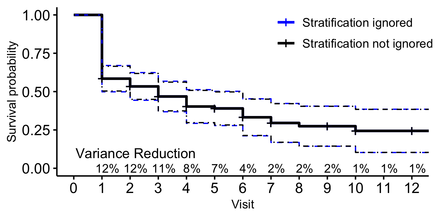
Figure 1: The K-M estimator of survival functions of NIDA-CTN-0044 treatment group. Dashed (dot-dashed) lines represent the estimates and confidence intervals if stratified randomization were (not) ignored in data analyses. “Variance Reduction” and the associated percentages represent the variance reduction by correcting the variance formula at each visit. The dashed and dot-dashed lines are very similar and almost coincide.

8 Discussion

Our asymptotics, as in many asymptotic results under the commonly used superpopulation inference framework for randomized trials, assume that the number of randomization strata is fixed and the number of participants in each stratum goes to infinity. This may be a reasonable approximation when no stratum has a small number of participants. In our data examples, the smallest stratum has 49 participants. An area of future research is to consider cases where some randomization strata have few participants.

In our data analysis of NIDA-CTN-0044, the stratification variable “treatment site” was not available in our data set. It was therefore neither used in the estimator nor in the corresponding variance estimate. The variance estimator (5) in this case is asymptotically conservative. This is because the outer expectation in the rightmost term of (4) is unchanged or decreased if $S$ is replaced by a coarsening of $S$ (defined as merging several randomization strata together in a preplanned way, in the analysis); this follows from the conditional Jensen’s inequality. This result may be useful more generally, e.g., when some strata are so small compared to the sample size that stratum-specific evaluation of the empirical means $E_{n}$ in (5) cannot be reliably done. In such cases a pre-planned, coarsened stratum indicator could be used and the resulting hypothesis test would still control Type I error, asymptotically.

Stratified randomization is related to stratified sampling designs, also called “two-phase sampling” (Sen,, 1988; Breslow and Wellner,, 2007; Bai et al.,, 2013). To the best of our knowledge, asymptotic results for these designs do not directly apply to our problem; a key difference is that asymptotic results for stratified sampling designs often involve finite population inference (commonly used in survey sampling), while here we use superpopulation inference (commonly used in analyzing randomized trials).

We provide R functions to calculate the variance for estimators including those in Examples 1-3 and the K-M estimator, which are available at https://github.com/BingkaiWang/covariate-adaptive.

References

- Andersen et al., (2012) Andersen, P. K., Borgan, O., Gill, R. D., and Keiding, N. (2012). Statistical Models Based on Counting Processes. Springer Science & Business Media.
- Austin et al., (2010) Austin, P., Manca, A., Zwarenstein, M., Juurlink, D., and Stanbrook, M. (2010). A substantial and confusing variation exists in handling of baseline covariates in randomized controlled trials: a review of trials published in leading medical journals. Journal of Clinical Epidemiology, 63(2):142 – 153.
- Bai et al., (2013) Bai, X., Tsiatis, A. A., and O’Brien, S. M. (2013). Doubly-robust estimators of treatment-specific survival distributions in observational studies with stratified sampling. Biometrics, 69(4):830–839.
- Breslow and Wellner, (2007) Breslow, N. E. and Wellner, J. A. (2007). Weighted likelihood for semiparametric models and two-phase stratified samples, with application to Cox regression. Scandinavian Journal of Statistics, 34(1):86–102.
- Bugni et al., (2018) Bugni, F. A., Canay, I. A., and Shaikh, A. M. (2018). Inference under covariate-adaptive randomization. Journal of the American Statistical Association, 113(524):1784–1796.
- Campbell et al., (2014) Campbell, A. N., Nunes, E. V., Matthews, A. G., Stitzer, M., Miele, G. M., Polsky, D., Turrigiano, E., Walters, S., McClure, E. A., Kyle, T. L., Wahle, A., Van Veldhuisen, P., Goldman, B., Babcock, D., Stabile, P. Q., Winhusen, T., and Ghitza, U. E. (2014). Internet-delivered treatment for substance abuse: A multisite randomized controlled trial. American Journal of Psychiatry, 171(6):683–690.
- Díaz et al., (2019) Díaz, I., Colantuoni, E., Hanley, D. F., and Rosenblum, M. (2019). Improved precision in the analysis of randomized trials with survival outcomes, without assuming proportional hazards. Lifetime Data Analysis, 25(3):439–468.
- Efron, (1971) Efron, B. (1971). Forcing a sequential experiment to be balanced. Biometrika, 58(3):403–417.
- EMA, (2015) EMA (2015). European Medicines Agency Guideline on Adjustment for Baseline Covariates in Clinical Trials. European Medicines Agency: CPMP/295050/2013.
- EMA, (2019) EMA (2019). Missing data in confirmatory clinical trials. Revision 1 - Adopted guideline. CPMP/EWP/1776/99 Rev. 1.
- FDA, (2019) FDA (2019). Adjusting for Covariates in Randomized Clinical Trials for Drugs and Biologics with Continuous Outcomes. Draft Guidance for Industry. https://www.fda.gov/media/123801/download.
- FDA, (2020) FDA (2020). COVID-19: Developing Drugs and Biological Products for Treatment or Prevention. Guidance for Industry. https://www.fda.gov/media/137926/download.
- FDA and EMA, (1998) FDA and EMA (1998). E9 statistical principles for clinical trials. U.S. Food and Drug Administration: CDER/CBER. European Medicines Agency: CPMP/ICH/363/96.
- Fleming and Harrington, (2011) Fleming, T. R. and Harrington, D. P. (2011). Counting Processes and Survival Analysis, volume 169. John Wiley & Sons.
- Kahan and Morris, (2012) Kahan, B. C. and Morris, T. P. (2012). Improper analysis of trials randomised using stratified blocks or minimisation. Statistics in Medicine, 31(4):328–340.
- Kaplan and Meier, (1958) Kaplan, E. L. and Meier, P. (1958). Nonparametric estimation from incomplete observations. Journal of the American Statistical Association, 53(282):457–481.
- Kosorok, (2008) Kosorok, M. R. (2008). Introduction to Empirical Processes and Semiparametric Inference. Springer.
- Lachin et al., (1988) Lachin, J., Matts, J., and Wei, L. (1988). Randomization in clinical trials: Conclusions and recommendations. Controlled Clinical Trials, 9(4):365 – 374.
- Li and Ding, (2019) Li, X. and Ding, P. (2019). Rerandomization and regression adjustment. arXiv, https://arxiv.org/abs/1906.11291.
- Lin et al., (2015) Lin, Y., Zhu, M., and Su, Z. (2015). The pursuit of balance: An overview of covariate-adaptive randomization techniques in clinical trials. Contemporary Clinical Trials, 45:21 – 25. 10th Anniversary Special Issue.
- Ling et al., (2009) Ling, W., Hillhouse, M., Domier, C., Doraimani, G., Hunter, J., Thomas, C., Jenkins, J., Hasson, A., Annon, J., Saxon, A., Selzer, J., Boverman, J., and Bilangi, R. (2009). Buprenorphine tapering schedule and illicit opioid use. Addiction, 104(2):256–265.
- Lu and Tsiatis, (2011) Lu, X. and Tsiatis, A. A. (2011). Semiparametric estimation of treatment effect with time-lagged response in the presence of informative censoring. Lifetime Data Analysis, 17(4):566–593.
- Ma et al., (2015) Ma, W., Hu, F., and Zhang, L. (2015). Testing hypotheses of covariate-adaptive randomized clinical trials. Journal of the American Statistical Association, 110(510):669–680.
- Ma et al., (2018) Ma, W., Qin, Y., Li, Y., and Hu, F. (2018). Statistical inference of covariate-adjusted randomized experiments. arXiv, https://arxiv.org/abs/1807.09678.
- Mallinckrodt et al., (2003) Mallinckrodt, C. H., Clark, W. S., Carroll, R. J., and Molenberghs, G. (2003). Assessing response profiles from incomplete longitudinal clinical trial data under regulatory considerations. Journal of Biopharmaceutical Statistics, 13(2):179–190. PMID: 12729388.
- (26) Moore, K. and van der Laan, M. (2009a). Covariate adjustment in randomized trials with binary outcomes: Targeted maximum likelihood estimation. Statistics in Medicine, 28(1):39–64.
- (27) Moore, K. L. and van der Laan, M. J. (2009b). Increasing power in randomized trials with right censored outcomes through covariate adjustment. Journal of Biopharmaceutical Statistics, 19(6):1099–1131. PMID: 20183467.
- Morgan and Rubin, (2012) Morgan, K. L. and Rubin, D. B. (2012). Rerandomization to improve covariate balance in experiments. The Annals of Statistics, 40(2):1263–1282.
- Neyman et al., (1990) Neyman, J. S., Dabrowska, D. M., and Speed, T. (1990). On the application of probability theory to agricultural experiments. essay on principles. section 9. Statistical Science, pages 465–472.
- Pocock and Simon, (1975) Pocock, S. J. and Simon, R. (1975). Sequential treatment assignment with balancing for prognostic factors in the controlled clinical trial. Biometrics, 31(1):103–115.
- Reid, (1981) Reid, N. (1981). Influence functions for censored data. The Annals of Statistics, pages 78–92.
- Robins, (2002) Robins, J. M. (2002). Covariance adjustment in randomized experiments and observational studies: Comment. Statistical Science, 17(3):309–321.
- Robins et al., (1994) Robins, J. M., Rotnitzky, A., and Zhao, L. P. (1994). Estimation of regression coefficients when some regressors are not always observed. Journal of the American Statistical Association, 89(427):846–866.
- Robins et al., (2007) Robins, J. M., Sued, M., Lei-Gomez, Q., and Rotnitzky, A. (2007). Comment: Performance of double-robust estimators when “inverse probability” weights are highly variable. Statistical Science, 22(4):544–559.
- Scharfstein et al., (1999) Scharfstein, D. O., Rotnitzky, A., and Robins, J. M. (1999). Adjusting for nonignorable drop-out using semiparametric nonresponse models. Journal of the American Statistical Association, 94(448):1096–1120.
- Sen, (1988) Sen, P. K. (1988). Asymptotics in finite population sampling. In Sampling, volume 6 of Handbook of Statistics, pages 291 – 331. Elsevier.
- Shao and Yu, (2013) Shao, J. and Yu, X. (2013). Validity of tests under covariate-adaptive biased coin randomization and generalized linear models. Biometrics, 69(4):960–969.
- Shao et al., (2010) Shao, J., Yu, X., and Zhong, B. (2010). A theory for testing hypotheses under covariate-adaptive randomization. Biometrika, 97(2):347–360.
- Shorack and Wellner, (2009) Shorack, G. R. and Wellner, J. A. (2009). Empirical Processes with Applications to Statistics. Society for Industrial and Applied Mathematics.
- Siddiqui et al., (2009) Siddiqui, O., Hung, H. M. J., and O’Neill, R. (2009). MMRM vs. LOCF: A Comprehensive Comparison Based on Simulation Study and 25 NDA Datasets. Journal of Biopharmaceutical Statistics, 19(2):227–246. PMID: 19212876.
- Steingrimsson et al., (2016) Steingrimsson, J., Hanley, D., and Rosenblum, M. (2016). Improving precision by adjusting for baseline variables in randomized trials with binary outcomes, without regression model assumptions. Contemporary Clinical Trials, 54:18–24.
- Tsiatis, (2007) Tsiatis, A. (2007). Semiparametric theory and missing data. Springer Science & Business Media.
- van der Laan and Gruber, (2012) van der Laan, M. J. and Gruber, S. (2012). Targeted minimum loss based estimation of causal effects of multiple time point interventions. The International Journal of Biostatistics, 8(1):Article 9.
- van der Vaart, (1998) van der Vaart, A. (1998). Asymptotic Statistics. Cambridge Series in Statistical and Probabilistic Mathematics. Cambridge University Press.
- Wei, (1978) Wei, L. J. (1978). The adaptive biased coin design for sequential experiments. The Annals of Statistics, 6(1):92–100.
- Weiss et al., (2011) Weiss, R. D., Potter, J. S., Fiellin, D. A., Byrne, M., Connery, H. S., Dickinson, W., Gardin, J., Griffin, M. L., Gourevitch, M. N., Haller, D. L., Hasson, A. L., Huang, Z., Jacobs, P., Kosinski, A. S., Lindblad, R., McCance-Katz, E. F., Provost, S. E., Selzer, J., Somoza, E. C., Sonne, S. C., and Ling, W. (2011). Adjunctive Counseling During Brief and Extended Buprenorphine-Naloxone Treatment for Prescription Opioid Dependence: A 2-Phase Randomized Controlled Trial. JAMA Psychiatry, 68(12):1238–1246.
- Yang and Tsiatis, (2001) Yang, L. and Tsiatis, A. (2001). Efficiency study of estimators for a treatment effect in a pretest-posttest trial. The American Statistician, 55(4):314–321.
- Ye and Shao, (2019) Ye, T. and Shao, J. (2019). Validity and robustness of tests in survival analysis under covariate-adaptive randomization. arXiv, https://arxiv.org/abs/1811.07232.
- Zelen, (1974) Zelen, M. (1974). The randomization and stratification of patients to clinical trials. Journal of Chronic Diseases, 27(7):365 – 375.
- Zhang, (2015) Zhang, M. (2015). Robust methods to improve efficiency and reduce bias in estimating survival curves in randomized clinical trials. Lifetime Data Analysis, 21(1):119–137.