Identification of Dominant Subspaces for Linear Structured Parametric Systems and Model Reduction

Abstract

In this paper, we discuss a novel model reduction framework for generalized linear systems. The transfer functions of these systems are assumed to have a special structure, e.g., coming from second-order linear systems and time-delay systems, and they may also have parameter dependencies. Firstly, we investigate the connection between classic interpolation-based model reduction methods with the reachability and observability subspaces of linear structured parametric systems. We show that if enough interpolation points are taken, the projection matrices of interpolation-based model reduction encode these subspaces. As a result, we are able to identify the dominant reachable and observable subspaces of the underlying system. Based on this, we propose a new model reduction algorithm combining these features leading to reduced-order systems. Furthermore, we pay special attention to computational aspects of the approach and discuss its applicability to a large-scale setting. We illustrate the efficiency of the proposed approach with several numerical large-scale benchmark examples.

15A69, 34C20, 41A05, 49M05, 93A15, 93C10, 93C15.

1 Introduction

In this paper, we consider linear structured parametric systems, whose transfer functions are of the form:

(1.1) $$\mathbf{H}(s,\mathbf{p})=\mathcal{C}(s,\mathbf{p})\mathcal{K}(s,\mathbf{p})^{-1}\mathcal{B}(s,\mathbf{p}),$$

where

(1.2) $$\mathcal{C}(s,\mathbf{p}) =\sum_{i=1}^{k}\gamma_{i}(s,\mathbf{p})\mathbf{C}_{i}, \mathcal{K}(s,\mathbf{p}) =\sum_{i=1}^{l}\kappa_{i}(s,\mathbf{p})\mathbf{A}_{i}, \mathcal{B}(s,\mathbf{p}) =\sum_{i=1}^{m}\beta_{i}(s,\mathbf{p})\mathbf{B}_{i},$$

in which $\mathbf{A}_{i}\in\mathbb{R}^{n\times n}$, $\mathbf{B}_{i}\in\mathbb{R}^{n\times m}$, $\mathbf{C}_{i}\in\mathbb{R}^{p\times n}$ are constant matrices, $s$ take values on the imaginary axis, and $\mathbf{p}=\begin{bmatrix}p^{(1)},\ldots,p^{(d)}\end{bmatrix}\in\Omega^{d}$ are the system parameters. $\kappa_{i}(s,\mathbf{p}),\beta_{i}(s,\mathbf{p})$ and $\gamma_{i}(s,\mathbf{p})$ are functions of $s\in\mathbb{C}$ and $\mathbf{p}\in\Omega^{d}$. Additionally, the restrictions $\kappa_{i}(\cdot,\mathbf{p}),\beta_{i}(\cdot,\mathbf{p})$ and $\gamma_{i}(\cdot,\mathbf{p})$ are assumed to be meromorphic functions. In this paper, we also assume that $\mathbf{H}(s,\mathbf{p})$ is a strictly proper function for all parameters, i.e., $\lim\limits_{s\rightarrow\pm i\infty}\mathbf{H}(s,\mathbf{p})=0$. The system (1.1) covers a large class of linear systems, arising in various science and engineering applications, e.g., classical linear systems, second-order systems, time-delay systems, integro-differential systems, and their parameter-dependent variants.

In order to illustrate the class of systems (1.1), we consider a dynamical system arising in computational electro-magnetics presented in [16]. A discretized system can be obtained by the spatial discretization of electromagnetic field equations, describing the electro-dynamical behavior of microwave devices when the surface losses are included in a physical model. The transfer function of the system has a very particular structure; precisely, it has a fractional integrator and takes the form:

(1.3) $$\mathbf{H}(s)=\sqrt{s}\mathbf{B}^{T}\left(s^{2}\mathbf{I}-\frac{1}{\sqrt{s}}\mathbf{D}+\mathbf{A}\right)^{-1}\sqrt{s}\mathbf{B}.$$

If the above equation is compared with the form given in Eq. 1.1 for a fixed parameter, then the matrices $\mathcal{C}(s),\mathcal{K}(s)$ and $\mathcal{B}(s)$ can be given by

$$\mathcal{C}(s)=\sqrt{s}\mathbf{B}^{T},\quad\mathcal{K}(s)=\left(s^{2}\mathbf{I}-\frac{1}{\sqrt{s}}\mathbf{D}+\mathbf{A}\right),\quad~{}\,~{}~{}\mathcal{B}(s)=\sqrt{s}\mathbf{B},$$

and

$$\gamma_{1}(s)=\beta_{1}(s)=\sqrt{s},\quad\kappa_{1}(s)=s^{2},\quad \kappa_{2}(s)=-\frac{1}{\sqrt{s}},\quad\kappa_{3}(s)\equiv 1,$$

$$\mathbf{B}_{1}=\mathbf{C}_{1}^{T}=\mathbf{B},\quad\mathbf{A}_{1}=\mathbf{I},\quad \mathbf{A}_{2}=\mathbf{D}\quad\text{and}~{}\,\mathbf{A}_{3}=\mathbf{A}.$$

Hence, the transfer function (1.3) fits into our framework (1.1).

Model order reduction (MOR) has been studied extensively in the literature for some classes of linear systems, see e.g., [2, 8] for standard linear systems, [9, 11, 14, 29] for second-order systems, [19, 28] for time-delay systems, and the review paper [7] for parametric systems. Furthermore, MOR techniques have been investigated by several researchers for the generalized linear systems (1.1). For a fixed parameter, balanced truncation has been proposed in [10]. The method requires solving the system Gramians, namely reachability and observability Gramians, which can be a computationally challenging task in a large-scale setting. Another popular MOR method, transfer function interpolation, has also been studied [3, 5], where for a given set of interpolation points, it is shown how to construct an interpolating reduced-order system while preserving the system structure. However, [3, 5] leave an important open problem about the choice of a good set of interpolation points. Furthermore, we would like to mention that a data-driven approach for structured non-parametric systems has been studied in [30]. Nevertheless, the construction of the structured reduced-order system is not a straightforward task; more importantly, it is not clear how to construct a reachable and observable system.

In this paper, we discuss the connection between interpolation-based MOR methods with the reachable and observable subspaces of linear structured parametric systems. We show that if enough interpolation points are taken, the projection matrices of interpolation-based model reduction encode these subspaces. As a consequence, we propose an approach to construct reduced-order systems preserving the common subspaces containing the most reachable as well as the most observable states. This approach can be seen as a combination of the interpolation-based method in [3] and some inspiration from the Loewner framework for first-order systems [23].

The precise structure of the paper is as follows. In the subsequent section, we discuss the construction of interpolating reduced-order systems for (1.1) for a given set of interpolation points $s$ and parameters $\mathbf{p}$. Thereafter, in Section 3 we define the concepts of reachability and observability for linear structured parametric systems and connect them with the interpolation-based MOR methods. Subsequently, by combining both features, we discuss the construction of reduced-order systems keeping the subspaces of the most reachable and observable states simultaneously. In Section 5, we illustrate the efficiency of the approach using several benchmark examples and finally conclude with future avenues. In the rest of the paper, we make use of the following notation.

• $\texttt{svd}\{\cdot\}$ denotes the singular value decomposition (SVD) of a matrix.

• By using MATLAB^® notation, we denote the first $l$ columns of a matrix $\mathbf{V}$ by $\mathbf{V}(:,1:l)$.

• Let $\mathcal{V}$ be a subspace of $\mathbb{C}^{n}$ (or $\mathbb{R}^{n}$). We denote the orthogonal subspace of $\mathcal{V}$ by $\mathcal{V}^{\perp}$.

2 Preliminary Work

In this section, we briefly recap an interpolatory framework to construct reduced-order systems. Let us consider linear systems whose input-output mappings (transfer functions) are given in (1.1). Our goal is to construct reduced-order systems having a similar structure using Petrov-Galerkin projection as follows:

(2.1) $$\mathbf{\hat{H}}(s,\mathbf{p})=\hat{\mathcal{C}}(s,\mathbf{p})\mathcal{\hat{K}}(s,\mathbf{p})^{-1}\mathcal{\hat{B}}(s,\mathbf{p}),$$

where

(2.2) $$\mathcal{\hat{C}}(s,\mathbf{p}) =\mathcal{C}(s,\mathbf{p})\mathbf{V}, \mathcal{\hat{K}}(s,\mathbf{p}) =\mathbf{W}^{T}\mathcal{K}(s,\mathbf{p})\mathbf{V}, \mathcal{\hat{B}}(s,\mathbf{p}) =\mathbf{W}^{T}\mathbf{B}(s,\mathbf{p})\mathbf{V}.$$

We aim at determining the matrices $\mathbf{V}$ and $\mathbf{W}$ in a way that the resulting reduced-order system interpolates a given set of interpolation points for $s$ and $\mathbf{p}$. This problem was considered in [3], where the idea of constructing interpolatory non-parametric structured systems [5] and classical linear parametric systems [4] was extended to the systems (2.1). However, the authors in [3] present the framework for linear structured parametric systems, where the functions given in (1.2) can be decomposed as $q(s,\mathbf{p}):=q_{s}(s)q_{p}(\mathbf{p})$. In the following theorem, we present a variation of this result where this decomposition is not required.

Theorem 2.1.

Let $\mathbf{H}(s,\mathbf{p})$ be a transfer function as in (1.1). Consider interpolation points $\{\sigma_{i},\mathbf{p}^{r}_{i}\}$ and $\{\mu_{i},\mathbf{p}^{l}_{i}\}$, $i\in\{1,\ldots,r\}$, such that $\mathcal{K}(s,\mathbf{p})$ is invertible for $\{s,\mathbf{p}\}\in\{\sigma_{i},\mathbf{p}_{i}^{r}\}\cup\{\mu_{i},\mathbf{p}_{i}^{l}\}$. Furthermore, let the projection matrices $\mathbf{V},\mathbf{W}\in\mathbb{C}^{n\times r}$ be as follows:

(2.3a) $$\underset{i=1,\ldots,r}{\mathop{\mathrm{span}}}\left\{\mathcal{K}(\sigma_{i},\mathbf{p}^{l}_{i})^{-1}\mathcal{B}(\sigma_{i},\mathbf{p}^{r}_{i})\right\} \subseteq\mathop{\mathrm{range}}\left(\mathbf{V}\right),$$

(2.3b) $$\underset{i=1,\ldots,r}{\mathop{\mathrm{span}}}\left\{\mathcal{K}(\mu_{i},\mathbf{p}^{r}_{i})^{-T}\mathcal{C}(\sigma_{i},\mathbf{p}^{l}_{i})^{T}\right\} \subseteq\mathop{\mathrm{range}}\left(\mathbf{W}\right).$$

If the reduced matrices are computed as shown in (2.2), then the following conditions are satisfied, for $i=1,\dots,r$:

(2.4a) $$\mathbf{H}(\sigma_{i},\mathbf{p}^{l}_{i}) =\mathbf{\hat{H}}(\sigma_{i},\mathbf{p}^{l}_{i}),$$

(2.4b) $$\mathbf{H}(\mu_{i},\mathbf{p}^{r}_{i}) =\mathbf{\hat{H}}(\mu_{i},\mathbf{p}^{r}_{i}).$$

Moreover, if $\mu_{i}=\sigma_{i}$, and $\mathbf{p}^{l}_{i}=\mathbf{p}^{r}_{i}=:\mathbf{p}_{i}$, for $i\in\{1,\ldots,r\}$, and $\mathbf{H}(s,\mathbf{p})$ and $\mathbf{\hat{H}}(s,\mathbf{p})$ are differentiable at $\sigma_{i}$ and $\mathbf{p}_{i}$ for $i\in\{1,\ldots,r\}$, then along with (2.4), the following conditions are satisfied:

(2.5a) $$\dfrac{d}{ds}\mathbf{H}(\sigma_{i},\mathbf{p}_{i}) =\dfrac{d}{ds}\mathbf{\hat{H}}(\sigma_{i},p_{i}),$$

(2.5b) $$\nabla_{\mathbf{p}}\mathbf{H}(\sigma_{i},\mathbf{p}_{i}) =\nabla_{\mathbf{p}}\mathbf{\hat{H}}(\sigma_{i},\mathbf{p}_{i}).$$

Proof 2.2.

The theorem can be proven exactly along the lines given in [3]. We begin by proving (2.4a). We have

$$\hat{}\mathbf{H}(\sigma_{i},\mathbf{p}^{l}_{i}) =\hat{}\mathcal{C}(\sigma_{i},\mathbf{p}^{l}_{i})\hat{}\mathcal{K}(\sigma_{i},\mathbf{p}^{l}_{i})^{-1}\hat{}\mathcal{B}(\sigma_{i},\mathbf{p}^{l}_{i})$$

$$=\mathcal{C}(\sigma_{i},\mathbf{p}^{l}_{i})\mathbf{V}\hat{}\mathcal{K}(\sigma_{i},\mathbf{p}^{l}_{i})^{-1}\mathbf{W}^{T}\mathcal{B}(\sigma_{i},\mathbf{p}^{l}_{i})$$

$$=\mathcal{C}(\sigma_{i},\mathbf{p}^{l}_{i})\mathbf{V}\hat{}\mathcal{K}(\sigma_{i},\mathbf{p}^{l}_{i})^{-1}\mathbf{W}^{T}\mathcal{K}(\sigma_{i},\mathbf{p}^{l}_{i})\underbrace{\mathcal{K}(\sigma_{i},\mathbf{p}^{l}_{i})^{-1}\mathcal{B}(\sigma_{i},\mathbf{p}^{l}_{i})}_{\in\mathop{\mathrm{range}}\left(\mathbf{V}\right)}$$

$$=\mathcal{C}(\sigma_{i},\mathbf{p}^{l}_{i})\mathbf{V}\hat{}\mathcal{K}(\sigma_{i},\mathbf{p}^{l}_{i})^{-1}\mathbf{W}^{T}\mathcal{K}(\sigma_{i},\mathbf{p}^{l}_{i})\mathbf{V}z$$

$$=\mathcal{C}(\sigma_{i},\mathbf{p}^{l}_{i})\mathbf{V}z=\mathcal{C}(\sigma_{i},\mathbf{p}^{l}_{i})\mathcal{K}(\sigma_{i},\mathbf{p}^{l}_{i})^{-1}\mathcal{B}(\sigma_{i},\mathbf{p}^{l}_{i})=\mathbf{H}(\sigma_{i},\mathbf{p}^{l}_{i}).$$

Analogously, we can prove (2.4b). Furthermore, we can prove (2.5a) and (2.5b) along the lines given in [5] and [4], respectively. For the sake of brevity, we refrain from providing a complete proof.

In the previous theorem, we have seen how an interpolatory reduced-order system can be constructed for a given set of interpolation points. However, a good choice of interpolation points for both frequency $(s)$ and the parameters $(\mathbf{p})$ remains an open question. Therefore, in this work, we show that for enough interpolation points, we can determine the important subspaces, leading to a good quality of reduced-order systems. For this, in what follows, we first discuss the concepts of reachability and observability for dynamical systems.

3 Reachability, Observability and Reduced-Order Systems

This section aims at showing the connection of the Petrov-Galerkin projection matrices $\mathbf{V}$ and $\mathbf{W}$ in (2.3) (Theorem 2.1) with the classical concepts of reachability and observability of dynamical systems. Based on this, we can identify the states that are simultaneously least reachable and least observable. This leads us to an algorithm which is a combination of interpolation and SVD techniques, enabling us to construct reduced-order systems for structured parametric systems. We begin here by briefly revisiting some results for first-order linear systems.

3.1 Background on First-order Systems

The transfer function of a first-order system is given by

(3.1) $$\mathbf{H}_{\texttt{fo}}(s)=\mathbf{C}\left(s\mathbf{I}-\mathbf{A}\right)^{-1}\mathbf{B},\quad\text{with~{}\,~{} $\mathbf{A}\in\mathbb{C}^{n\times n}$, $\mathbf{B}\in\mathbb{C}^{n\times m}$ and $\mathbf{C}\in\mathbb{C}^{p\times n}$.}$$

We note that the reachable subspace $\mathcal{V}_{\scaleto{{R}}{3.25pt}}$ and the observable subspace $\mathcal{W}_{\scaleto{{O}}{3.25pt}}$ of the system (3.1) are given by the smallest subspaces of $\mathbb{C}^{n}$ such that

$$e^{\mathbf{A}t}\mathbf{B}\in\mathcal{V}_{\scaleto{{R}}{3.25pt}}\quad\text{and}\quad e^{\mathbf{A}^{T}t}\mathbf{C}^{T}\in\mathcal{W}_{\scaleto{{O}}{3.25pt}}~{}\,\text{for every $t\geq 0$.}$$

This essentially follows from standard proofs relating reachability and observability of linear-time invariant systems with the rank of the Kalman reachability and observability matrices defined as follows:

(3.2a) $$\mathbf{M}_{\scaleto{{R}}{3.25pt}}(\mathbf{A},\mathbf{B}) =\begin{bmatrix}\mathbf{B}&\mathbf{A}\mathbf{B}&\mathbf{A}^{2}\mathbf{B}&\dots&\mathbf{A}^{n-1}\mathbf{B}\end{bmatrix},\,~{}\text{and}$$

(3.2b) $$~{}\,\mathbf{M}_{\scaleto{{O}}{3.25pt}}^{T}(\mathbf{C},\mathbf{A}) =\begin{bmatrix}\mathbf{C}^{T}&\mathbf{A}^{T}\mathbf{C}^{T}&(\mathbf{A}^{2})^{T}\mathbf{C}^{T}&\dots&(\mathbf{A}^{n-1})^{T}\mathbf{C}^{T}\end{bmatrix},$$

see [13, Chapter 2] for more details. The unreachable subspace, which is the orthogonal complement of $\mathcal{V}_{\scaleto{{R}}{3.25pt}}$ and denoted by $\mathcal{V}_{\scaleto{{R}}{3.25pt}}^{\perp}$, consists of the states $\mathbf{q}_{ur}\in\mathbb{C}^{n}$ such that $\mathbf{q}_{ur}^{T}e^{\mathbf{A}t}\mathbf{B}=0$ for every $t\geq 0$. Similarly, the unobservable subspace, characterized by $\mathcal{W}_{\scaleto{{O}}{3.25pt}}^{\perp}$, consists of the states $\mathbf{q}_{uo}\in\mathbb{C}^{n}$ such that $\mathbf{C}e^{\mathbf{A}t}\mathbf{q}_{uo}=0$, for every $t\geq 0$. By means of the Laplace transform, the reachability and observability subspaces can be seen as the smallest subspaces of $\mathbb{C}^{n}$ such that

(3.3) $$(s\mathbf{I}-\mathbf{A})^{-1}\mathbf{B}\in\mathcal{V}_{\scaleto{{R}}{3.25pt}},\quad\text{and}\quad(s\mathbf{I}-\mathbf{A})^{-T}\mathbf{C}^{T}\in\mathcal{W}_{\scaleto{{O}}{3.25pt}},~{}\,\text{for every $s\in i\mathbb{R}$.}$$

Additionally, we note that the system (3.1) is reachable if $\mathcal{V}_{\scaleto{{R}}{3.25pt}}=\mathbb{C}^{n}$, and observable if $\mathcal{W}_{\scaleto{{O}}{3.25pt}}=\mathbb{C}^{n}$. A classical result in system theory is that if the system (3.1) is not reachable or not observable, then there exists a system of lower-order, having the same transfer function as the original one. Indeed, the unreachable or unobservable states, denoted by $\mathcal{V}_{\scaleto{{R}}{3.25pt}}^{\perp}$ and $\mathcal{W}_{\scaleto{{O}}{3.25pt}}^{\perp}$, respectively, can be removed from the dynamics, without changing the transfer function. Moreover, if the system is reachable and observable, then it is minimal, i.e., there exists no lower-order realization for the original transfer function, see [13, Chapter 2].

For first-order systems, a well-known characterization of reachable and observable spaces are given by $\mathcal{V}_{\scaleto{{R}}{3.25pt}}=\mathop{\mathrm{range}}\left(\mathbf{M}_{\scaleto{{R}}{3.25pt}}(\mathbf{A},\mathbf{B})\right)$ and $\mathcal{W}_{\scaleto{{O}}{3.25pt}}=\mathop{\mathrm{range}}\left(\mathbf{M}_{\scaleto{{O}}{3.25pt}}^{T}(\mathbf{C},\mathbf{A})\right),$ where $\mathbf{M}_{\scaleto{{R}}{3.25pt}}(\mathbf{A},\mathbf{B})$ and $\mathbf{M}_{\scaleto{{O}}{3.25pt}}^{T}(\mathbf{C},\mathbf{A})$ are, respectively, the Kalman reachability and observability matrices given in (3.2). Furthermore, the authors in [1] provided a different characterization of these subspaces which is closely related to the interpolation problem. In particular, they have shown that $\mathcal{V}_{\scaleto{{R}}{3.25pt}}=\mathop{\mathrm{range}}\left(\mathbf{V}\right)$ and $\mathcal{W}_{\scaleto{{O}}{3.25pt}}=\mathop{\mathrm{range}}\left(\mathbf{W}\right)$, where

$$\mathbf{V} =\begin{bmatrix}(\sigma_{1}\mathbf{I}-\mathbf{A})^{-1}\mathbf{B}&(\sigma_{2}\mathbf{I}-\mathbf{A})^{-1}\mathbf{B}&\dots&(\sigma_{N}\mathbf{I}-\mathbf{A})^{-1}\mathbf{B}\end{bmatrix},~{}\text{and}$$

$$\mathbf{W} =\begin{bmatrix}(\sigma_{1}\mathbf{I}-\mathbf{A})^{-T}\mathbf{C}^{T}&(\sigma_{2}\mathbf{I}-\mathbf{A})^{-T}\mathbf{C}^{T}&\dots&(\sigma_{N}\mathbf{I}-\mathbf{A})^{-T}\mathbf{C}^{T}\end{bmatrix}$$

with $N\geq n$ and $\sigma_{k}\in i\mathbb{R}\cap\Lambda(\mathbf{A}),k\in\{1,\ldots,N\}$, are distinct points, where $\Lambda(\cdot)$ denotes the spectrum of a matrix. Notice that the above matrices $\mathbf{V}$ and $\mathbf{W}$ are the particular matrices $\mathbf{V}$ and $\mathbf{W}$ from Theorem 2.1 when the original system is first-order non-parametric. Moreover, also in [1] and more recently in [23], the authors have shown that the matrix $\begin{bmatrix}\mathbf{W}^{T}\mathbf{V}&\mathbf{W}^{T}\mathbf{A}\mathbf{V}\end{bmatrix}$ encodes the dimension of the minimal order realization of the original system, i.e.,

$$\mathop{\mathrm{rank}}\left(\begin{bmatrix}\mathbf{W}^{T}\mathbf{V}&\mathbf{W}^{T}\mathbf{A}\mathbf{V}\end{bmatrix}\right)=\left\{\begin{array}[]{l}\text{order of the minimal realization obtained by}\\ \text{removing unreachable and unobservable states}\end{array}\right.$$

Furthermore, in [23], an algorithm based on the SVD is provided in order to get the minimal realization or reduced-order systems by Petrov-Galerkin projections.

Inspired by the above discussion on first-order systems, in what follows, we first extend some of the results for linear structured systems (1.1), and propose an algorithm, allowing us to construct reduced-order systems by removing unreachable and unobservable subspaces.

3.2 Reachability, Observability, and Reduced Systems for Linear Structured Systems

As mentioned earlier, unreachable or unobservable states can be removed from first-order systems (3.1) such that the resulting lower-order system has the same transfer function as the original one. In this section, we study how these notions can be extended to the class of structured systems (1.1). For the clarity of exposition, we start our discussion with the non-parametric case, i.e., linear structured systems of the form

(3.4) $$\mathbf{H}(s)=\mathcal{C}(s)\mathcal{K}(s)^{-1}\mathcal{B}(s).$$

Dynamical systems can be represented using different frameworks, e.g., as a semi-group in a Hilbert space, as a linear system over a ring of operators and as a functional differential equation. Depending on the nature of representation or the considered problem, there exist various definitions for reachability and observability.

For the infinite-dimensional control community, dynamical systems are represented in the infinite-dimensional setting, where the state-space might be seen as an (infinite-dimensional) Hilbert space associated with a semi-group. There, the notions of exact and approximate reachability and observability play an important role, see, e.g., [17, 34] and [12, Chapter 4]. However, in this setup, the dynamical systems are no longer seen as functional differential equations. Hence, discretizing the infinite-dimensional Hilbert space leads to finite-dimensional first-order reduced-order systems that do not preserve the structure in (1.1).

Another point of view is the one in algebraic system theory, which considers dynamical systems as linear systems over a ring, see, e.g., [20, 21]. In this setting, the reachability and observability concepts rely on a rank condition over a ring, e.g., strong and weak reachability/observability, see [22, 27, 31]. However, since these concepts depend on the underlying ring, we are not aware of a way to adapt it to a structure-preserving reduction in the Petrov-Galerkin projection framework.

In this paper, we define a weaker notion of reachability/observability that relies only on linear algebra concepts and the matrices of the realization of the system (3.4). These concepts are related to the realization of the transfer function (3.4) as a functional differential equation, see [10, 18].

Definition 3.1.

The $\mathbb{C}^{n}$–reachable subspace $\mathcal{V}_{\scaleto{{R}}{3.25pt}}$ associated to the pair of functions $(\mathcal{K}(s),\mathcal{B}(s))$ is the smallest subspace of $\mathbb{C}^{n}$ which contains $\mathcal{K}(s)^{-1}\mathcal{B}(s)$ for all $s\in i\mathbb{R}$. In other words, if $\mathcal{V}_{\scaleto{{R}}{3.25pt}}=\mathop{\mathrm{range}}\left(\mathbf{V}_{\scaleto{{R}}{3.25pt}}\right)$, where $\mathbf{V}_{\scaleto{{R}}{3.25pt}}\in\mathbb{C}^{n\times r_{\scaleto{{R}}{3.25pt}}}$ is a full column rank matrix and $r_{\scaleto{{R}}{3.25pt}}\leq n$, we have

(3.5) $$\mathcal{K}(s)^{-1}\mathcal{B}(s)=\mathbf{V}_{\scaleto{{R}}{3.25pt}}y_{\scaleto{{R}}{3.25pt}}(s),$$

in which $y_{\scaleto{{R}}{3.25pt}}(s)\in\mathbb{C}^{r_{\scaleto{{R}}{3.25pt}}\times m}$ is a matrix of meromorphic function. We say that $(\mathcal{K}(s),\mathcal{B}(s))$ is $\mathbb{C}^{n}$–reachable if $\mathcal{V}_{\scaleto{{R}}{3.25pt}}=\mathbb{C}^{n}$.

The $\mathbb{C}^{n}$–unreachable subspace consists of the states $\mathbf{q}_{ur}\in\mathbb{C}^{n}$ such that

$$\mathbf{q}_{ur}^{T}\mathcal{K}(s)^{-1}\mathcal{B}(s)=0\quad\forall s\in i\mathbb{R}.$$

As a consequence, it is characterized by $\mathcal{V}_{\scaleto{{R}}{3.25pt}}^{\perp}$. It is worth noting that, in the case of first-order systems (3.1), $\mathcal{K}(s)^{-1}\mathcal{B}(s)=(s\mathbf{I}-\mathbf{A})^{-1}\mathbf{B}$ and the above definition is a natural extension of (3.3).

We recall that the transfer between the input to the state for system (3.4) is given by

$$\mathbf{x}(s)=\mathcal{K}(s)^{-1}\mathcal{B}(s)\mathbf{u}(s).$$

Hence, the $\mathbb{C}^{n}$–reachable subspace $\mathcal{V}_{\scaleto{{R}}{3.25pt}}$ correspond to the smallest subspace that contains the states $\mathbf{x}(s)$ for every $s$. This justifies the use of the reachability terminology.

To connect the frequency and time-domains, let $\mathbf{M}(t)$ denote the inverse Laplace transform of $\mathcal{K}(s)^{-1}\mathcal{B}(s)$. Hence, by definition $\mathbf{M}(t)=\mathbf{V}_{\scaleto{{R}}{3.25pt}}\mathbf{Y}(t)$ $\forall t\geq 0$, where $\mathbf{Y}(t)$ is the inverse Laplace transform of $y_{\scaleto{{R}}{3.25pt}}(s)$ in (3.5). It can be noticed that, for real systems, i.e., systems where $\mathbf{M}(t)$ is a real function, the matrix $\mathbf{V}_{\scaleto{{R}}{3.25pt}}$ can be chosen as a real matrix. Also, in the context of time-delay systems, Definition 3.1 is equivalent to the one of point-wise complete controllability, see [35, 36] and of $\mathbb{R}^{n}$ controllability [20, Chapter 2]. Similarly, we use the following concept of observability.

Definition 3.2.

The $\mathbb{C}^{n}$–observable subspace $\mathcal{W}_{\scaleto{{O}}{3.25pt}}$ associated to the pair of functions $(\mathcal{C}(s),\mathcal{K}(s))$ is the smallest subspace of $\mathbb{C}^{n}$ which contains $\mathcal{K}(s)^{-T}\mathcal{C}(s)^{T}$, for all $s\in i\mathbb{R}$. In other words, if $\mathcal{W}_{\scaleto{{O}}{3.25pt}}=\mathop{\mathrm{range}}\left(\mathbf{W}_{\scaleto{{O}}{3.25pt}}\right)$ , where $\mathbf{W}_{\scaleto{{O}}{3.25pt}}\in\mathbb{C}^{n\times r_{\scaleto{{O}}{3.25pt}}}$ is a full rank matrix and $r_{\scaleto{{O}}{3.25pt}}\leq n$, we have

$$\mathcal{C}(s)\mathcal{K}(s)^{-1}=y_{\scaleto{{O}}{3.25pt}}(s)\mathbf{W}_{\scaleto{{O}}{3.25pt}}^{T},$$

in which $y_{\scaleto{{O}}{3.25pt}}(s)\in\mathbb{C}^{p\times r_{\scaleto{{O}}{3.25pt}}}$ is a matrix of meromorphic functions. We say that $(\mathcal{C}(s),\mathcal{K}(s))$ is $\mathbb{C}^{n}$–observable if $\mathcal{W}_{\scaleto{{O}}{3.25pt}}=\mathbb{C}^{n}$.

The $\mathbb{C}^{n}$–unobservable subspace consists of the states $\mathbf{q}_{uo}\in\mathbb{C}^{n}$ such that

$$\mathcal{C}(s)\mathcal{K}(s)^{-1}\mathbf{q}_{uo}=0\quad\forall s\in i\mathbb{R}.$$

As a consequence, it is characterized by $\mathcal{W}_{\scaleto{{O}}{3.25pt}}^{\perp}$. Similarly, in the case of first-order systems (3.1), $\mathcal{K}(s)^{-T}\mathcal{C}^{T}(s)=(s\mathbf{I}-\mathbf{A})^{-T}\mathbf{C}^{T}$ and the above definition is a natural extension of (3.3) for observability. As for the $\mathbb{C}^{n}$ reachability space, $\mathbf{W}_{\scaleto{{O}}{3.25pt}}$ can be chosen to be real if the original system represents a real dynamics.

Analogous to first-order systems (3.1), if a structured system (3.4) is not $\mathbb{C}^{n}$–reachable or $\mathbb{C}^{n}$–observable, there exists a lower-order system that has the same transfer function. We state the result rigorously in the following theorem.

Theorem 3.3.

Let $(\mathcal{C}(s),\mathcal{K}(s),\mathcal{B}(s))$ be a linear structured system of order $n$ as shown in (3.4). If either $(\mathcal{C}(s),\mathcal{K}(s))$ is not $\mathbb{C}^{n}$–observable or $(\mathcal{K}(s),\mathcal{B}(s))$ is not $\mathbb{C}^{n}$–reachable, then there exists a lower-order structured realization $(\mathcal{\hat{C}}(s),\mathcal{\hat{K}}(s),\mathcal{\hat{B}}(s))$ of order $r<n$, realizing the original transfer function, i.e.,

$$\mathcal{C}(s)\mathcal{K}(s)^{-1}\mathcal{B}(s)=\mathcal{\hat{C}}(s)\mathcal{\hat{K}}(s)^{-1}\mathcal{\hat{B}}(s),\quad\forall s\in i\mathbb{R}.$$

Proof 3.4.

Let us first consider the case where the structured system is not $\mathbb{C}^{n}$–reachable. In this case, there exists a full rank matrix $\mathbf{V}_{\scaleto{{R}}{3.25pt}}\in\mathbb{C}^{n\times r_{\scaleto{{R}}{3.25pt}}}$ such that $\mathcal{K}(s)^{-1}\mathcal{B}(s)=\mathbf{V}_{\scaleto{{R}}{3.25pt}}z(s)$. Consider a matrix $\mathbf{W}\in\mathbb{R}^{n\times r_{\scaleto{{R}}{3.25pt}}}$ and assume that $\mathbf{W}^{T}\mathcal{K}(s)\mathbf{V}_{\scaleto{{R}}{3.25pt}}$ is non-singular. Hence, $(\mathbf{W}^{T}\mathcal{K}(s)^{-1}\mathbf{V}_{\scaleto{{R}}{3.25pt}})^{-1}\mathbf{W}^{T}\mathcal{B}(s)=z(s)$ and we have

(3.6) $$\mathcal{K}(s)^{-1}\mathcal{B}(s)=\mathbf{V}_{\scaleto{{R}}{3.25pt}}(\mathbf{W}^{T}\mathcal{K}(s)^{-1}\mathbf{V}_{\scaleto{{R}}{3.25pt}})^{-1}\mathbf{W}^{T}\mathcal{B}(s).$$

Thus,

$$\mathcal{C}(s)\mathcal{K}(s)^{-1}\mathcal{B}(s)=\hat{\mathcal{C}}(s)\hat{\mathcal{K}}(s)^{-1}\hat{\mathcal{B}}(s)$$

with

$$\hat{\mathcal{C}}(s)=\mathcal{C}(s)\mathbf{V}_{\scaleto{{R}}{3.25pt}}\in\mathbb{C}^{p\times r},~{}\,\hat{\mathcal{K}}(s)=\mathbf{W}^{T}\mathcal{K}(s)\mathbf{V}_{\scaleto{{R}}{3.25pt}}\in\mathbb{C}^{r\times r},~{}\,\text{and}~{}\,\hat{\mathcal{B}}(s)=\mathbf{W}^{T}\mathcal{B}(s)\in\mathbb{C}^{r\times m}.$$

Similarly, when the system is not $\mathbb{C}^{n}$–observable, it can be shown that there exists a lower-order realization.

The above result states that if a structured realization is not $\mathbb{C}^{n}$–reachable or $\mathbb{C}^{n}$–observable, then there exists a lower-order structured realization which represents the same transfer function. Moreover, a lower-order realization can be obtained via Petrov-Galerkin projections. Although the counterpart of Theorem 3.3 is valid for first-order systems as (3.1), until now we have not been able to give a concrete proof for this result for structured systems. Hence, we leave the following statement as a conjecture.

Conjecture 3.1.

Let $(\mathcal{C}(s),\mathcal{K}(s),\mathcal{B}(s))$ be a linear structured system of order $n$ as given in (3.4). If $(\mathcal{C}(s),\mathcal{K}(s))$ is $\mathbb{C}^{n}$–observable and $(\mathcal{K}(s),\mathcal{B}(s))$ is $\mathbb{C}^{n}$–reachable, then there is no lower-order realization, which can be constructed via Petrov-Galerkin projection that realizes the same transfer function.

Remark 3.5.

For first-order systems (3.1), 3.1 is equivalent to the statement that a system is minimal if and only if it is reachable and observable. Its proof is based on the Markov parameters of the system, which are represented by $\mathbf{C}\mathbf{A}^{k}\mathbf{B}\in\mathbb{C}^{p\times m}$ for $k\geq 0$, and the associated Hankel matrix, see, e.g., [13, Theorem 2.28]. However, in the structured parametric case, the classical Markov parameters $\mathbf{M}_{k}\in\mathbb{C}^{p\times m}$, where $\mathbf{H}(s)=\sum_{k=0}^{\infty}\mathbf{M}_{k}/s^{k}$, give information about the first-order realization as (3.1) which realizes the transfer function $\mathbf{H}(s)$. Hence, they are incompetent to the understanding of the structured minimal realization. Additionally, the Markov parameters considered in the algebraic system theory depend on $s$ and $\mathbf{p}$ and are no longer elements of $\mathbb{C}^{p\times m}$, see [20]. Hence, a similar argument as for first-order systems does not hold here. For the moment, we let this be a potential research problem, and we will dedicate future work in the direction of finding a good framework where classical linear systems results can be extended to the structured parametric case.

We have shown that if we know reachable and observable subspaces $\mathcal{V}_{\scaleto{{R}}{3.25pt}}$ and $\mathcal{W}_{\scaleto{{O}}{3.25pt}}$, we are able to construct lower-order systems by removing the states that are unreachable or unobservable. The next step is to characterize these spaces using matrices $\mathbf{V}$ and $\mathbf{W}$ defined in Theorem 2.1. By definition, it is easy to observe that $\mathop{\mathrm{range}}\left(\mathbf{V}\right)\subseteq\mathcal{V}_{\scaleto{{R}}{3.25pt}}$ and $\mathop{\mathrm{range}}\left(\mathbf{W}\right)\subseteq\mathcal{W}_{\scaleto{{O}}{3.25pt}}$. Additionally, there always exist $N\in\mathbb{N}$ and interpolation points $\sigma_{1},\dots,\sigma_{N}$ such that

(3.7a) $$\mathbf{V} =\begin{bmatrix}\mathcal{K}(\sigma_{1})^{-1}\mathcal{B}(\sigma_{1})&\mathcal{K}(\sigma_{2})^{-1}\mathcal{B}(\sigma_{2})&\dots&\mathcal{K}(\sigma_{N})^{-1}\mathcal{B}(\sigma_{N})\end{bmatrix},$$

(3.7b) $$\mathbf{W} =\begin{bmatrix}\mathcal{K}(\sigma_{1})^{-T}\mathcal{C}(\sigma_{1})^{T}&\mathcal{K}(\sigma_{2})^{-T}\mathcal{C}(\sigma_{2})^{T}&\dots&\mathcal{K}(\sigma_{N})^{-T}\mathcal{C}(\sigma_{N})^{T}\end{bmatrix},$$

and

$$\mathop{\mathrm{range}}\left(\mathbf{V}\right)=\mathcal{V}_{\scaleto{{R}}{3.25pt}}\quad\text{and}\quad\mathop{\mathrm{range}}\left(\mathbf{W}\right)=\mathcal{W}_{\scaleto{{O}}{3.25pt}}.$$

In what follows, we show that $N$ can be fixed in some cases where the following assumption holds.

Assumption 3.1 (at most $n_{z}$ zeros on the imaginary axis).

Given $n_{z}\in\mathbb{N}$ and the functions $\mathcal{K}(s)$ and $\mathcal{B}(s)$, we say that the pair of functions $(\mathcal{K}(s),\mathcal{B}(s))$ has at most $n_{z}$ zeros on the imaginary axis, with $n_{z}\in\mathbb{N}$, if, for every $\mathbf{w}\in\mathbb{C}^{n}$ and $\mathbf{z}\in\mathbb{C}^{m}$, the scalar meromorphic function

$$\mathbf{F}_{\mathbf{w},\mathbf{z}}(s)=\mathbf{w}^{T}\mathcal{K}(s)^{-1}\mathcal{B}(s)\mathbf{z}$$

has at most $n_{z}$ zeros on the imaginary axis.

Hence, the following theorem is an extension of the result for first-order systems from [1, Lemma 3.1] to linear structured systems.

Theorem 3.6.

Let $(\mathcal{K}(s),\mathcal{B}(s))$ be a pair of matrix functions whose reachable subspace is $\mathcal{V}_{\scaleto{{R}}{3.25pt}}$. Let us assume that the pair $(\mathcal{K}(s),\mathcal{B}(s))$ has at most $n_{z}$ zeros on the imaginary axis. Let

$$\mathbf{V}=\begin{bmatrix}\mathcal{K}(\sigma_{1})^{-1}\mathcal{B}(\sigma_{1})&\mathcal{K}(\sigma_{2})^{-1}\mathcal{B}(\sigma_{2})&\dots&\mathcal{K}(\sigma_{N})^{-1}\mathcal{B}(\sigma_{N})\end{bmatrix},$$

with $N\geq n_{z}$. Hence,

$$\mathcal{V}_{\scaleto{{R}}{3.25pt}}=\mathop{\mathrm{range}}\left(\mathbf{V}_{\scaleto{{R}}{3.25pt}}\right)=\mathop{\mathrm{range}}\left(\mathbf{V}\right).$$

Proof 3.7.

Suppose that $\mathcal{K}(s)^{-1}\mathcal{B}(s)$ has at most $n_{z}$ zeros on $i\mathbb{R}$. We know that $\mathop{\mathrm{range}}\left(\mathbf{V}\right)\subseteq\mathcal{V}_{\scaleto{{R}}{3.25pt}}$. Suppose by contradiction that $\mathop{\mathrm{range}}\left(\mathbf{V}\right)\neq\mathcal{V}_{\scaleto{{R}}{3.25pt}}$. Hence, there exists a vector $\mathbf{w}\in\mathcal{V}_{\scaleto{{R}}{3.25pt}}$ such that $\mathbf{w}^{T}\mathbf{V}=0$. Hence, $\mathbf{w}^{T}\mathcal{K}(\sigma_{j})^{-1}\mathcal{B}(\sigma_{j})e_{i}=0$, for $j=1,\dots,N$, $i=1,\dots,m$. Hence, the function $\mathbf{w}^{T}\mathcal{K}(s)^{-1}\mathcal{B}(s)e_{i}=0$ has at least $N$ zeros on the imaginary axis, with $N\geq n_{z}$, which contradicts the assumption of $n_{z}$ zeros.

Theorem 3.6 shows that, under the hypothesis of a limited number of zeros on the imaginary axis, the reachability subspace is encoded by the matrix $\mathbf{V}$ constructed with $N$ interpolation points, where $N\geq n_{z}$.

Remark 3.8.

In order to have $n_{z}$ from Theorem 3.6, 3.1 needs to be fulfilled. However, this assumption is difficult to verify in practice. Nevertheless, numerical experiments show that it is enough to choose $N=n$, so that $\mathop{\mathrm{range}}\left(\mathbf{V}\right)=\mathcal{V}_{\scaleto{{R}}{3.25pt}}$. Moreover, in a large-scale setting $(n\in\mathcal{O}(10^{5}{-}10^{6}))$, we observe that as we increase the number of interpolation points $(N)$, $\mathop{\mathrm{range}}\left(\mathbf{V}\right)\to\mathcal{V}_{\scaleto{{R}}{3.25pt}}$.

The same analysis presented here holds for the observability space.

3.3 Note on the Parametric Case

So far, we have presented the definitions of $\mathbb{C}^{n}$ reachability and $\mathbb{C}^{n}$ observability for structured non-parametric systems. For the parametric case (1.1), we can consider the following natural extensions of Definitions 3.1 and 3.2. The reachable subspace $\mathcal{V}_{\scaleto{{R}}{3.25pt}}=\mathop{\mathrm{range}}\left(\mathbf{V}_{\scaleto{{R}}{3.25pt}}\right)$ associated to the pair of functions $(\mathcal{K}(s,\mathbf{p}),\mathcal{B}(s,\mathbf{p}))$, with a full column rank matrix $\mathbf{V}_{\scaleto{{R}}{3.25pt}}\in\mathbb{C}^{n\times r_{\scaleto{{R}}{3.25pt}}}$, $r_{\scaleto{{R}}{3.25pt}}\leq n$, is the smallest subspace of $\mathbb{C}^{n}$ which contains $\mathcal{K}(s,\mathbf{p})^{-1}\mathcal{B}(s,\mathbf{p})$ for every $s\in i\mathbb{R}$ and $\mathbf{p}\in\Omega^{d}$. In other words,

$$\mathcal{K}(s,\mathbf{p})^{-1}\mathcal{B}(s,\mathbf{p})=\mathbf{V}_{\scaleto{{R}}{3.25pt}}\mathbf{z}_{c}(s,\mathbf{p}),$$

where $\mathbf{z}_{c}(s,\mathbf{p})\in\mathbb{C}^{p\times r_{\scaleto{{R}}{3.25pt}}}$. Similarly, the $\mathbb{C}^{n}$–observable subspace $\mathcal{W}_{\scaleto{{O}}{3.25pt}}=\mathop{\mathrm{range}}\left(\mathbf{W}_{\scaleto{{O}}{3.25pt}}\right)$ associated to $(\mathcal{C}(s,\mathbf{p}),\mathcal{K}(s,\mathbf{p}))$, with a full rank matrix $\mathbf{W}_{\scaleto{{O}}{3.25pt}}\in\mathbb{C}^{n\times r_{\scaleto{{O}}{3.25pt}}}$, $r_{\scaleto{{O}}{3.25pt}}\leq n$, is the smallest subspace of $\mathbb{C}^{n}$ which contains $\mathcal{K}(s,\mathbf{p})^{-T}\mathcal{C}(s,\mathbf{p})^{T}$ for every $s\in i\mathbb{R}$ and $\mathbf{p}\in\Omega^{d}$. In other words,

$$\mathcal{C}(s,\mathbf{p})\mathcal{K}(s,\mathbf{p})^{-1}=y_{\scaleto{{O}}{3.25pt}}(s,\mathbf{p})\mathbf{W}^{T}\mathbf{W}_{\scaleto{{O}}{3.25pt}},$$

where $y_{\scaleto{{O}}{3.25pt}}(s,\mathbf{p})\in\mathbb{C}^{p\times r_{\scaleto{{O}}{3.25pt}}}$ is a matrix of functions. Furthermore, the result of Theorem 3.3 can be extended to the parametric case, showing that states that are unreachable and unobservable can be removed. We do not have an analogue for Theorem 3.6. However, we know that if we take enough interpolations points $(\sigma_{i},\mathbf{p}_{i})$, the matrices

(3.8a) $$\mathbf{V} =\begin{bmatrix}\mathcal{K}(\sigma_{1},\mathbf{p}_{1})^{-1}\mathcal{B}(\sigma_{1},\mathbf{p}_{1})&\dots&\mathcal{K}(\sigma_{N},\mathbf{p}_{N})^{-1}\mathcal{B}(\sigma_{N},\mathbf{p}_{N)}\end{bmatrix},$$

(3.8b) $$\mathbf{W} =\begin{bmatrix}\mathcal{K}(\sigma_{1},\mathbf{p}_{1})^{-T}\mathcal{C}(\sigma_{1},\mathbf{p}_{1})^{T}&\dots&\mathcal{K}(\sigma_{N},\mathbf{p}_{N})^{-T}\mathcal{C}(\sigma_{N},\mathbf{p}_{N})^{T}\end{bmatrix},$$

encode the reachability and observability spaces, i.e.,

$$\mathop{\mathrm{range}}\left(\mathbf{V}\right)=\mathcal{V}_{\scaleto{{R}}{3.25pt}}\quad\text{and}\quad\mathop{\mathrm{range}}\left(\mathbf{W}\right)=\mathcal{W}_{\scaleto{{O}}{3.25pt}}.$$

From now on, we assume that we have enough interpolation points such that $\mathop{\mathrm{range}}\left(\mathbf{V}\right)=\mathcal{V}_{\scaleto{{R}}{3.25pt}}$ and $\mathop{\mathrm{range}}\left(\mathbf{W}\right)=\mathcal{W}_{\scaleto{{O}}{3.25pt}}$.

3.4 Simultaneous Reduction

We have seen that if the system (1.1) is not reachable or not observable, there exists a lower-order realization whose transfer function remains the same as the original one. To obtain such a lower-order realization, one needs to truncate the states that are unreachable and observable, as shown in Theorem 3.3. However, it remains an open question of how this information can be used to obtain reduced-order systems. In what follows, we propose a method enabling to identify simultaneously the states that are unreachable and unobservable. For this, we assume that

(3.9) $$\mathop{\mathrm{rank}}\left(\begin{bmatrix}\mathbf{W}^{T}\mathbf{A}_{1}\mathbf{V}&\dots&\mathbf{W}^{T}\mathbf{A}_{l}\mathbf{V}\end{bmatrix}\right)=\mathop{\mathrm{rank}}\left(\begin{bmatrix}\mathbf{W}^{T}\mathbf{A}_{1}\mathbf{V}\\ \vdots\\ \mathbf{W}^{T}\mathbf{A}_{l}\mathbf{V}\end{bmatrix}\right)=r,$$

where $\mathbf{V}$ and $\mathbf{W}$ are the matrices defined in Eq. 3.7 encoding, respectively, the reachability and the observability subspaces, i.e., $\mathop{\mathrm{range}}\left(\mathbf{V}\right)=\mathcal{V}_{\scaleto{{R}}{3.25pt}}$ and $\mathop{\mathrm{range}}\left(\mathbf{W}\right)=\mathcal{W}_{\scaleto{{O}}{3.25pt}}$ and $\mathbf{A}_{i},i\in\{1,\ldots,l\}$, are defined in (1.2). Then, we consider the compact SVDs

(3.10) $$\begin{bmatrix}\mathbf{W}^{T}\mathbf{A}_{1}\mathbf{V}&\dots&\mathbf{W}^{T}\mathbf{A}_{l}\mathbf{V}\end{bmatrix}=\mathbf{W}_{1}\Sigma_{l}\tilde{\mathbf{V}}^{T}\quad\text{and}\quad\begin{bmatrix}\mathbf{W}^{T}\mathbf{A}_{1}\mathbf{V}\\ \vdots\\ \mathbf{W}^{T}\mathbf{A}_{l}\mathbf{V}\end{bmatrix}=\tilde{\mathbf{W}}\Sigma_{r}\mathbf{V}_{1}^{T}.$$

Let $\mathbf{W}_{p}:=\mathbf{W}\mathbf{W}_{1}$ and $\mathbf{V}_{p}:=\mathbf{V}\mathbf{V}_{1}$ be two projection matrices and let us consider the lower-order realization $\mathcal{\hat{C}}_{p}(s,\mathbf{p})\mathcal{\hat{K}}_{p}(s,\mathbf{p})^{-1}\mathcal{\hat{B}}_{p}(s,\mathbf{p})$ constructed by Petrov-Galerkin projection as follows:

(3.11) $$\mathcal{\hat{B}}_{p}(s,\mathbf{p})=\mathbf{W}_{p}^{T}\mathcal{B}(s,\mathbf{p}),\quad\mathcal{\hat{C}}_{p}(s,\mathbf{p})=\mathcal{C}(s,\mathbf{p})\mathbf{V}_{p},\quad\mathcal{\hat{K}}_{p}(s,\mathbf{p})=\mathbf{W}_{p}^{T}\mathcal{K}(s,\mathbf{p})\mathbf{V}_{p}.$$

Then, the following result holds.

Theorem 3.9.

The lower-order system $\mathcal{\hat{C}}_{p}(s,\mathbf{p})\mathcal{\hat{K}}_{p}(s,\mathbf{p})^{-1}\mathcal{\hat{B}}_{p}(s,\mathbf{p})$ of order $r$, obtained as given in Eq. 3.11, realizes the original transfer function, i.e.,

$$\mathcal{\hat{C}}_{p}(s,\mathbf{p})\mathcal{\hat{K}}_{p}(s,\mathbf{p})^{-1}\mathcal{\hat{B}}_{p}(s,\mathbf{p})=\mathcal{C}(s,\mathbf{p})\mathcal{K}(s,\mathbf{p})^{-1}\mathcal{B}(s,\mathbf{p})$$

for every $s\in i\mathbb{R}$ and $\mathbf{p}\in\Omega^{d}$.

Proof 3.10.

Recall that $\mathbf{V}_{p}=\mathbf{V}\mathbf{V}_{1}$ and $\mathbf{W}_{p}=\mathbf{W}\mathbf{W}_{1}$. Hence, by construction, $\mathop{\mathrm{range}}\left(\mathbf{V}_{p}\right)\subseteq\mathop{\mathrm{range}}\left(\mathbf{V}\right)=\mathcal{V}_{\scaleto{{R}}{3.25pt}}$ and $\mathop{\mathrm{range}}\left(\mathbf{W}_{p}\right)\subseteq\mathop{\mathrm{range}}\left(\mathbf{W}\right)=\mathcal{W}_{\scaleto{{O}}{3.25pt}}$. Hence, there exist $\mathbf{V}_{a}$ and $\mathbf{W}_{a}$, $\mathbf{V}_{a}\perp\mathbf{V}_{p}$ and $\mathbf{W}_{a}\perp\mathbf{W}_{p}$ such that $\mathop{\mathrm{range}}\left(\begin{bmatrix}\mathbf{V}_{p}&\mathbf{V}_{a}\end{bmatrix}\right)=\mathcal{V}_{\scaleto{{R}}{3.25pt}}$ and $\mathop{\mathrm{range}}\left(\begin{bmatrix}\mathbf{W}_{p}&\mathbf{W}_{a}\end{bmatrix}\right)=\mathcal{W}_{\scaleto{{O}}{3.25pt}}$. As a consequence, from the compact SVDs in (3.10),

$$\mathbf{W}^{T}\mathbf{A}_{k}\mathbf{V}_{a}=0,\quad\mathbf{W}_{a}^{T}\mathbf{A}_{k}\mathbf{V}=0,\quad\text{and}\quad\mathbf{W}_{a}^{T}\mathbf{A}_{k}\mathbf{V}_{a}=0,~{}\text{for $k=1,\dots,l$},$$

and hence,

$$\mathbf{W}_{p}^{T}\mathcal{K}(s,\mathbf{p})\mathbf{V}_{a}=0,\quad\mathbf{W}_{a}^{T}\mathcal{K}(s,\mathbf{p})\mathbf{V}_{p}=0,\quad\text{and}~{}\,\quad\mathbf{W}_{a}^{T}\mathcal{K}(s,\mathbf{p})\mathbf{V}_{a}=0.$$

Moreover, notice that

$$\mathcal{K}(s,\mathbf{p})^{-1}\mathcal{B}(s,\mathbf{p})=\begin{bmatrix}\mathbf{V}_{p}&\mathbf{V}_{a}\end{bmatrix}\begin{bmatrix}\mathcal{\hat{K}}_{p}(s,\mathbf{p})^{-1}\mathcal{\hat{B}}_{p}(s,\mathbf{p})\\ \star\end{bmatrix}\quad\text{and}$$

$$\mathcal{C}(s,\mathbf{p})\mathcal{K}(s,\mathbf{p})^{-1}=\begin{bmatrix}\mathcal{\hat{C}}_{p}(s,\mathbf{p})\mathcal{\hat{K}}_{p}(s,\mathbf{p})^{-1}&\star\end{bmatrix}\begin{bmatrix}\mathbf{W}_{p}^{T}\\ \mathbf{W}_{a}^{T}\end{bmatrix}.$$

Finally, we write

$$\mathcal{C}(s,\mathbf{p}) \mathcal{K}(s,\mathbf{p})^{-1}\mathcal{B}(s,\mathbf{p})=\mathcal{C}(s,\mathbf{p})\mathcal{K}(s)^{-1}\mathcal{K}(s,\mathbf{p})\mathcal{K}(s,\mathbf{p})^{-1}\mathcal{B}(s,\mathbf{p})$$

$$=\begin{bmatrix}\mathcal{\hat{C}}(s,\mathbf{p})\mathcal{\hat{K}}(s,\mathbf{p})^{-1}&\star\end{bmatrix}\begin{bmatrix}\mathbf{W}_{p}^{T}\\ \mathbf{W}_{a}^{T}\end{bmatrix}\mathcal{K}(s,\mathbf{p})\begin{bmatrix}\mathbf{V}_{p}&\mathbf{V}_{a}\end{bmatrix}\begin{bmatrix}\mathcal{\hat{K}}(s,\mathbf{p})^{-1}\mathcal{\hat{B}}(s,\mathbf{p})\\ \star\end{bmatrix}$$

$$=\begin{bmatrix}\mathcal{\hat{C}}(s,\mathbf{p})\mathcal{\hat{K}}(s,\mathbf{p})^{-1}&\star\end{bmatrix}\begin{bmatrix}\mathbf{W}_{p}^{T}\mathcal{K}(s,\mathbf{p})\mathbf{V}_{p}&0\\ 0&0\end{bmatrix}\begin{bmatrix}\mathcal{\hat{K}}(s,\mathbf{p})^{-1}\mathcal{\hat{B}}(s,\mathbf{p})\\ \star\end{bmatrix}$$

$$=\mathcal{\hat{C}}(s,\mathbf{p})\mathcal{\hat{K}}(s,\mathbf{p})^{-1}\mathcal{\hat{K}}(s,\mathbf{p})\mathcal{\hat{K}}(s,\mathbf{p})^{-1}\mathcal{\hat{B}}(s,\mathbf{p})=\mathcal{\hat{C}}(s,\mathbf{p})\mathcal{\hat{K}}(s,\mathbf{p})^{-1}\mathcal{\hat{B}}(s,\mathbf{p}),$$

which concludes the proof.

Theorem 3.9 shows that if we construct the lower-order system as shown in Eq. 3.11, it also realizes the original system. As a consequence, the rank condition Eq. 3.9 gives us the order $r$ of the lower-order realization constructed by Petrov Galerkin projection which realizes the original system. Hence, the matrices

(3.12) $$\begin{bmatrix}\mathbf{W}^{T}\mathbf{A}_{1}\mathbf{V}&\dots&\mathbf{W}^{T}\mathbf{A}_{l}\mathbf{V}\end{bmatrix},\quad\text{and}~{}\,\begin{bmatrix}\mathbf{W}^{T}\mathbf{A}_{1}\mathbf{V}\\ \vdots\\ \mathbf{W}^{T}\mathbf{A}_{l}\mathbf{V}\end{bmatrix}$$

encode the complexity of the original system. Moreover, by means of the compact SVDs of these matrices, we are able to find the projection matrices $\mathbf{V}_{p}=\mathbf{V}\mathbf{V}_{1}$ and $\mathbf{W}_{p}=\mathbf{W}\mathbf{W}_{1}$, leading to a lower-order system having the same transfer function as the original one. Hence, the states that are removed from the dynamics of the original systems can be seen as unreachable or unobservable ones. On the other hand, the singular values in $\Sigma_{r}$ and $\Sigma_{l}$ give some important information about the simultaneous degree of reachability and observability of the states. Indeed, states that are related to small singular values can be interpreted to have a weak simultaneous degree of reachability and observability, while the states related to large singular values are strongly simultaneously reachable and observable. Therefore, removing also the subspaces associated with small singular values leads to reduced-order systems.

4 Model-Order Reduction Algorithm

Based on the arguments given in the previous section, we propose Algorithm 4.1 enabling us to construct reduced-order systems for structured systems (3.4). The procedure consists in selecting interpolation points $(s_{i},\mathbf{p}_{i})$ and constructs the matrices $\mathbf{V}$ and $\mathbf{W}$ as in (2.3) (steps 2 and 3). If we have enough interpolation points, the subspaces $\mathop{\mathrm{range}}\left(\mathbf{V}\right)$ and $\mathop{\mathrm{range}}\left(\mathbf{W}\right)$ mimic the reachable subspace $\mathcal{V}_{\scaleto{{R}}{3.25pt}}$ and the observable $\mathcal{W}_{\scaleto{{O}}{3.25pt}}$, respectively. Then, in step 4, we compute the SVDs of the matrices in (4.1). As previously discussed, the numerical rank of those matrices gives the order of a good reduced-order system. Hence, in step 5, the projection matrices $\mathbf{V}_{p}$ and $\mathbf{W}_{p}$ are constructed according to Theorem 3.9. Finally, in step 6, the reduced-order system is determined by Petrov-Galerkin projection.

Remark 4.1.

So far in the paper, we have refrained from discussing the idea of tangential interpolation. In the case of multi-input multi-output (MIMO) systems, one can employ the idea of tangential interpolation which has been proven to be very useful in MIMO case. For this, along with considering interpolation points $\{\sigma_{i},\mathbf{p}^{r}_{i}\}$ and $\{\mu_{j},\mathbf{p}^{l}_{j}\}$, we also consider tangential directions $\mathbf{b}_{i}$ and $\mathbf{c}_{j}$ of appropriate sizes. For details, we refer to e.g., [4]. Hence, with the tangential directions, the analogues of matrices $\mathbf{V}$ and $\mathbf{W}$ in (3.8) are

$$\mathbf{V} =\begin{bmatrix}\mathcal{K}(\sigma_{1},\mathbf{p}_{1})^{-1}\mathcal{B}(\sigma_{1},\mathbf{p}_{1})\mathbf{b}_{1}&\dots&\mathcal{K}(\sigma_{N},\mathbf{p}_{N})^{-1}\mathcal{B}(\sigma_{N},\mathbf{p}_{N)}\mathbf{b}_{N}\end{bmatrix},$$

$$\mathbf{W} =\begin{bmatrix}\mathcal{K}(\sigma_{1},\mathbf{p}_{1})^{-T}\mathcal{C}(\sigma_{1},\mathbf{p}_{1})^{T}\mathbf{c}_{1}^{T}&\dots&\mathcal{K}(\sigma_{N},\mathbf{p}_{N})^{-T}\mathcal{C}(\sigma_{N},\mathbf{p}_{N})^{T}\mathbf{c}_{N}^{T}\end{bmatrix}.$$

Hence, these matrices can be used in step 3 of Algorithm 4.1.

Remark 4.2.

One of the additional advantages of the proposed algorithm is that it inherently allows us to construct frequency-limited reachable and observable subspaces by choosing the interpolation points in a given frequency range. Hence, it yields a reduced-order system that is good in the considered frequency range.

Remark 4.3.

The proposed framework is also suitable for non-dynamical linear parametric systems, i.e., systems of the form

$$\mathbf{A}(\mathbf{p})\mathbf{x}(\mathbf{p}) =\mathbf{B}(\mathbf{p}),$$

$$\mathbf{y}(\mathbf{p}) =\mathbf{C}(\mathbf{p})\mathbf{x}(\mathbf{p}).$$

In this case, the solution $\mathbf{y}(\mathbf{p})$ can be obtained as

$$\mathbf{y}(\mathbf{p})=\mathbf{C}(\mathbf{p})\mathbf{A}(\mathbf{p})^{-1}\mathbf{B}(\mathbf{p}),$$

and the reachability and observability subspaces, namely $\mathcal{V}_{\scaleto{{R}}{3.25pt}}$ and $\mathcal{W}_{\scaleto{{O}}{3.25pt}}$, are the smallest subspaces such that $\mathbf{A}(\mathbf{p})^{-1}\mathbf{B}(\mathbf{p})\in\mathcal{V}_{\scaleto{{R}}{3.25pt}}$ and $\mathbf{A}(\mathbf{p})^{-T}\mathbf{C}(\mathbf{p})^{T}\in\mathcal{W}_{\scaleto{{O}}{3.25pt}}$ for all $\mathbf{p}\in\Omega^{d}$. In this case, we determine dominant subsystems with respect to parameters using the Algorithm 4.1.

Remark 4.4.

In several applications, it is highly desirable to determine reduced-order systems via one-sided projection in order to potentially preserve some important properties of the systems such as stability or passivity. In this case, in step 3 of Algorithm 4.1, we set $\mathbf{W}=\mathbf{V}$, and in step 5 of Algorithm 4.1, we again set $\mathbf{W}_{p}=\mathbf{V}_{p}$.

Algorithm 4.1 Construction of ROMs via Dominant Reachable and Observable subspace-based Projection (DROP).

1:Input: The transfer function as in (2.1), and order of reduced system $r$.

2:Choose left and right interpolation points for frequency and parameters.

3:Compute $\mathbf{V}$ and $\mathbf{W}$ using the interpolation points as in (2.3).

4:Determine SVDs

(4.1) $$\begin{bmatrix}\mathbf{W}^{T}\mathbf{A}_{1}\mathbf{V}&\dots&\mathbf{W}^{T}\mathbf{A}_{l}\mathbf{V}\end{bmatrix}=\mathbf{W}_{1}\Sigma_{l}\tilde{\mathbf{V}}^{T}\quad\text{and}\quad\begin{bmatrix}\mathbf{W}^{T}\mathbf{A}_{1}\mathbf{V}\\ \vdots\\ \mathbf{W}^{T}\mathbf{A}_{l}\mathbf{V}\end{bmatrix}=\tilde{\mathbf{W}}\Sigma_{r}\mathbf{V}_{1}^{T}$$

5:Compute projection matrices: $\mathbf{V}_{p}=\mathbf{V}\mathbf{V}_{1}(:,1:r)$ and $\mathbf{W}_{p}=\mathbf{W}\mathbf{W}_{1}(:,1:r)$.

6:Compute reduced matrices:

7:$\hat{\mathcal{K}}(s,\mathbf{p})=\mathbf{W}_{p}^{T}\mathcal{K}_{s}(s)\mathbf{V}_{p}$, $\hat{\mathcal{B}}(s,\mathbf{p})=\mathbf{W}_{p}^{T}\mathcal{B}(s,\mathbf{p})$ and $\hat{\mathcal{C}}(s,\mathbf{p})=\mathcal{C}(s,\mathbf{p})\mathbf{V}_{p}$.

8:Output: The reduced-order matrices: $\hat{\mathcal{K}}(s,\mathbf{p}),\hat{\mathcal{B}}(s,\mathbf{p}),$ and $\hat{\mathcal{C}}(s,\mathbf{p})$.

5 Numerical Results

In this section, we illustrate the efficiency of the proposed methods via several numerical examples, arising in various applications. We also compare for the non-parametric case with the existing methods proposed in [10, 16], and for the parametric case with the adaptive interpolation method proposed in [15]. We have performed all the simulations on a board with 4 Intel^® Xeon^® E7-8837 CPUs with a 2.67-GHz clock speed using MATLAB 8.0.0.783 (R2016b). Furthermore, we generate random numbers, whenever necessary, using rng(0,‘twister’). In the case of a MIMO system, we determine the projection matrices by employing the idea of tangential interpolation, and we choose the tangential directions randomly.

5.1 A Demo Example

At first, we discuss an artificial example to illustrate the proposed methods. Let us consider a system of order $n=3$ as follows:

(5.1) $$\begin{bmatrix}1&0&0\\ 0&1&0\\ 0&0&1\end{bmatrix}\dot{\mathbf{x}}(t) =\begin{bmatrix}-2&0&0\\ 0&-1&0\\ 0&0&-2\end{bmatrix}\mathbf{x}(t)+\mathbf{p}\begin{bmatrix}0&1&0\\ -1&0&0\\ 1&0&0\end{bmatrix}\mathbf{x}(t)+\begin{bmatrix}1\\ 0\\ 1\end{bmatrix}\mathbf{u}(t),$$

$$\mathbf{y}(t) =\begin{bmatrix}1&1&0\end{bmatrix}\mathbf{x}(t).$$

The example is constructed in such a way that the parameter $\mathbf{p}$ changes the imaginary parts of two eigenvalues of the system. Hence, with a change of the parameter, we expect a change in the peak of the transfer function.

Next, we aim at constructing a reduced realization of the system Eq. 5.1 by employing Algorithm 4.1. For this, we take $10$ points for the frequency $s\in\begin{bmatrix}10^{-4},10\end{bmatrix}$ and for the parameter $\mathbf{p}\in\begin{bmatrix}-10,10\end{bmatrix}$. We take the frequency points in the given range in the logarithm scale, whereas the parameters are chosen randomly in the considered parameter range. In Figure 5.1, we plot the decay of the singular values as shown in step $4$ of Algorithm 4.1. It can be observed that after the first two singular values, the singular values are at the level of machine precision. This means that a reachable and observable system, representing the input/output behavior of the system (5.1) has the order exactly $r=2$. We compare the transfer functions of the original and reduced-order systems for $20$ linearly spaced parameter values in $\begin{bmatrix}-10,10\end{bmatrix}$, which are plotted in Figure 5.2. The figure shows that the error between the original and reduced-order system is of the level of machine precision.

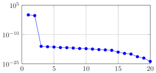
Figure 5.1: Demo example: Decay of the singular values.

The order 2 of a minimal realization can also be easily verified by analyzing the system (5.1). Notice that $x_{3}(t)$ does not influence the dynamics of $x_{1}(t)$ and $x_{2}(t)$, where $x_{i}(t)$ denotes the $i$th component of the vector $x(t)$, and $x_{3}(t)$ is not being observed since the output matrix $\mathbf{C}=\begin{bmatrix}1,1,0\end{bmatrix}$. Hence, $x_{3}(t)$ can be eliminated as far as the input-output dynamics are concerned. Therefore, the system (5.1) can exactly be reduced to order $2$.

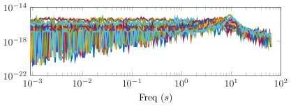
Figure 5.2: Demo example: The figure shows the Bode plot of the error between the original and reduced-order systems for different parameter values.

5.2 Time-Delay System

Next, we consider the time-delay model [5] of order $n$ as follows:

(5.2) $$\mathbf{E}\dot{\mathbf{x}}(t) =\mathbf{A}\mathbf{x}(t)+\mathbf{A}_{\tau}\mathbf{x}(t-\tau)+\mathbf{B}\mathbf{u}(t),$$

$$\mathbf{y}(t) =\mathbf{C}\mathbf{x}(t),$$

where $\mathbf{E}=\mu\mathbf{I}_{n}+\mathbf{T}$, $\mathbf{A}=\tfrac{1}{\tau}\left(\tfrac{1}{\zeta}+1\right)\left(\mathbf{T}-\mu\mathbf{I}_{n}\right)$, and $\mathbf{A}_{\tau}=\tfrac{1}{\tau}\left(\tfrac{1}{\zeta}-1\right)\left(\mathbf{T}-\mu\mathbf{I}_{n}\right)$ in which the matrix $\mathbf{T}$ is such that it is ones on the sub- and super-diagonal along with the $(1,1)$ and $(n,n)$ elements. The input matrix $\mathbf{B}$ is zero everywhere except for the first and second entries, i.e., $\mathbf{B}(1)=\mathbf{B}(2)=1$, and the output matrix is $\mathbf{C}=\mathbf{B}^{T}$. Furthermore, we choose $\mu=5$, $\zeta=0.01$, $\tau=1$, and the order $n=500$.

Next, we aim at constructing reduced-order systems using balanced truncation as proposed in [10] and using Algorithm 4.1. In order to apply Algorithm 4.1, we take $1000$ logarithmically distributed frequency points in the range $\begin{bmatrix}10^{-2},10^{4}\end{bmatrix}$. Furthermore, to apply balanced truncation, we need to determine the system Gramians, which are given in integral forms. To compute approximations of the Gramians, we make of use of quadv command in MATLAB with $\texttt{tol}=10^{-10}$ to integrate in the given frequency range.

First, we plot the singular values, obtained from balanced truncation and Algorithm 4.1 in Figure 5.3, which indicates a faster decay of singular values obtained from Algorithm 4.1. We now determine reduced-order systems of order $r=12$ using both methods. We compare the Bode plots of the original and reduced-order systems in Figure 5.4. The figure shows that both methods capture the dynamics very well; however, our method clearly yields a better reduced-order system at least by two orders of magnitudes.

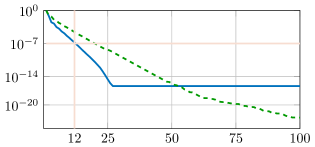
Figure 5.3: Time-delay example: Relative decay of the singular values using Algorithm 4.1 and structured balanced truncation.

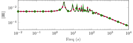
(a) The Bode plots of the original and reduced-order systems.

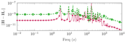
(b) The Bode plots of the errors of the reduced-order systems.

Figure 5.4: Time-delay example: The figure presents a comparison of the Bode plots of the original and reduced-order systems.

5.3 Heat Equation with Fading Memory

We consider the heat equation with fading memory presented in [10]. The example arises within the context of heat conduction in materials with fading memory. Its dynamics is governed by the following integro-PDE:

(5.3) $$\begin{split}v_{t}(t,x)&=\nabla v(t,x)-\int_{0}^{t}\gamma(t-s)\nabla v(s,x)ds+\chi_{\omega}\mathbf{u}(t)~{}\quad\text{in $(0,\infty)\times\Omega$},\\ v(t,x)&=0\quad\text{in $(0,\infty)\times\Gamma$},\qquad v(0,x)=0\quad\text{in $\Omega$},\\ v_{obs}(\cdot)&=\int_{\Omega}v(\cdot,x)dx,\end{split}$$

where $\gamma=1.05$, $\Omega=(0,1)\times(0,1)$, $\Gamma$ denotes the boundary of $\Omega$ and $\chi_{\omega}$ is the characteristic function of the control set $\omega=[0.15,0.25]\times[0.2,0.3]\subset\Omega$, i.e.,

$$\chi_{\omega}(x):=\begin{cases}1,\quad\text{if $x\in\omega$},\\ 0,\quad\text{otherwise}.\end{cases}$$

As discussed in [10], after spatial discretization by a finite difference method, we obtain a Volterra integro-differential system whose transfer function is given by

(5.4) $$\mathbf{H}(s)=\mathbf{C}\left(s\mathbf{I}-\mathbf{A}+\frac{1}{s+\gamma}\mathbf{A}\right)^{-1}\mathbf{B}.$$

We consider $128$ grid points in each direction, leading to a system of order $n=16,384$. In Figure 5.5, we first plot the relative singular values obtained using Algorithm 4.1 and balanced truncation from [10]. The figure shows that a very low-order model is possible to obtain having very high accuracy. We determine reduced-order systems of order $r=3$ using both methods. We compare both reduced-order systems in Figure 6(a), which shows that the reduced-order systems are comparable. Moreover, in Figure 6(b), we show the $\mathcal{H}_{2}$-norm of the error systems with respect to the order of the reduced-order system. This also indicates that both methods produce reduced-order systems of very similar quality.

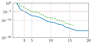
Figure 5.5: Heat equation with fading memory: Relative decay of the singular values using Algorithm 4.1 and structured balanced truncation.

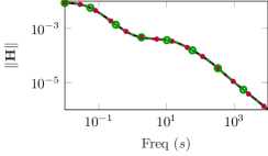
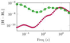
(a) The Bode plots of the original, reduced-order systems, and the error system.

(b) The Bode plots of the relative errors of the reduced-order systems.

Figure 5.6: Heat equation with fading memory: The figure presents a comparison of the Bode plots of the original and reduced-order systems for order $r=3$, and $\mathcal{H}_{2}$-norm of the error with respect to the order of the reduced-order systems.

5.4 Fractional Maxwell equations

Next, we consider the example mentioned in the introduction arising in computational electromagnetics, see [16]. As described in the introduction, the transfer function of this example has a fractional integrator of the form:

(5.5) $$\mathbf{H}(s)=s\mathbf{B}^{T}\left(s^{2}\mathbf{I}-\frac{1}{\sqrt{s}}\mathbf{D}+\mathbf{A}\right)^{-1}\mathbf{B},$$

where $n=29,295$ is the order, $\mathbf{I},\mathbf{A}$ and $\mathbf{D}$ are $n\times n$ matrices and $\mathbf{B}$ is a $1\times n$ matrix. This example is a limited frequency range and the interesting frequency range is $\mathcal{F}:=\begin{bmatrix}4e9,8e9\end{bmatrix}$Hz. We aim at employing Algorithm 4.1 and balanced truncation. Although the proposed balanced truncation [10] is not designed for limited frequency range, one can integrate within $\mathcal{F}$ range instead of $\begin{bmatrix}0,\infty\end{bmatrix}$ to determine the Gramians. However, we observe that for this example, the methodology proposed in [10] to obtain an approximation in low-rank factor does not converge. As discussed in [10], the development of low-rank solvers for Gramians of structure systems needs some future research which is highly relevant to this. Moreover, since the example is a large-scale one, it is not possible to apply the simple quadv function to obtain approximations of Gramians as we did in the delay example.

We instead compare our methodology to the method proposed in [16], where a reduced-order system is obtained using moment-matching based on a single expansion point. In order to employ Algorithm 4.1, we take $50$ points in the logarithm scale in the frequency range of interest. First, we plot the relative decay of the singular values in Figure 5.7. Ideally, we would like to determine a reduced-order system of order $r=38$, which is reported in [16]. However, our decay of singular values indicates that the order more than $10$ would not improve the quality of the reduced-order system as the singular values go to the level of machine precision. Therefore, we determine the reduced-order system of order $r=8$ via our method and compare with the reduced-order system of order $r=38$ as constructed in [16]. In Fig. 5.8, we compare both reduced-order systems. The figure suggests that our reduced-order systems outperformed the one reported in [16]. Importantly, notice that this is achieved even though our reduced-order system has an order more than four times smaller than the one from [16].

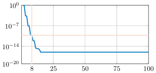
Figure 5.7: Fractional Maxwell equations: Relative decay of the singular values using Algorithm 4.1.

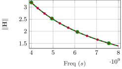
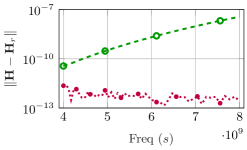
Figure 5.8: Fractional Maxwell equations: The Bode plots of the original, reduced-order systems, and the error system.

5.5 Parametric Anemometer

An anemometer, also known as a thermal mass flow meter, has sensors, namely heater and temperature after and before the heater in the direction of the flow as shown in Figure 5.9. Due to the circulation of the flow, a temperature difference occurs between the sensors. Measuring the temperature difference allows us to estimate the fluid flow, for more details see [24].

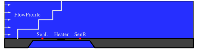
Figure 5.9: Schematic diagram of a two-dimensional anemometer, cf. [32].

The dynamics of the anemometer is governed by the convention-diffusion PDE as follows:

(5.6) $$\rho c\dfrac{\partial T}{\partial t}=\nabla\cdot\left(\kappa\nabla T\right)-\rho cv\nabla T+\dot{q},$$

where $\rho$ represents the mass density; $c$, $\kappa$, $v$ are the specific heat, thermal conductivity, and fluid velocity, respectively. Moreover, $\dot{q}$ denotes the heat flow into the system caused by the heater. We set $\rho=1$ and consider all other fluid properties as parameters. A discretization of the PDE leads to a parametric system whose transfer function is given as follows:

$$\mathbf{H}(s,\mathbf{p})=\mathbf{C}\left(s\left(\mathbf{E}_{0}+p_{1}\mathbf{E}_{1}\right)-\left(\mathbf{A}_{0}+p_{2}\mathbf{A}_{1}+p_{3}\mathbf{A}_{2}\right)\right)^{-1}\mathbf{B},$$

where $\mathbf{p}\in\mathbb{R}^{3}$ and $p_{i}$ denotes the $i$th component of the vector $\mathbf{p}$, which is given in terms of the fluid properties as follows:

$$\mathbf{p}=\begin{bmatrix}p_{1}\\ p_{2}\\ p_{3}\end{bmatrix}=\begin{bmatrix}c\\ \kappa\\ cv\end{bmatrix}.$$

The output matrix $\mathbf{C}$ is chosen such that it yields the output as the difference between the two sensors. For more details, we refer to [26] and for the model, to [32]. A finite-element discretization yields a parametric model of order $n=29,008$, and the model essentially has three parameters.

In order to apply the proposed method, we take $300$ points for frequency $s$ in the logarithmic way and $300$ random points for the parameters. For frequency, we consider the range $\begin{bmatrix}10^{1},10^{5}\end{bmatrix}$, and the parameters are generally considered in the intervals: $c\in\begin{bmatrix}0,1\end{bmatrix}$, $\kappa\in\begin{bmatrix}1,2\end{bmatrix}$, and $v\in\begin{bmatrix}0.1,2\end{bmatrix}$. First, in Figure 5.10, we plot the singular values, obtained by employing Algorithm 4.1, which exhibits a rapid decay. We now determine reduced-order systems of order $r=78$, meaning that we consider the singular vectors corresponding to the relative singular values up-to $10^{-6}$. We compare the Bode plots of the original and reduced-order systems in Figure 5.11 for two different parameter values, which clearly match for both parameters all frequencies.

Moreover, in Fig. 5.12, we plot the Bode diagram of the error systems, the difference of the original and reduced-order systems, for different parameter configurations. The obtained reduced-order system captures the dynamics of the original systems very well. From the figures, it can be seen that the error is below $2\cdot 10^{-7}$ for all frequencies and four considered parameter configurations.

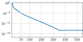
Figure 5.10: Anemometer example: relative decay of the singular values using Algorithm 4.1.

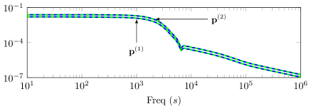
Figure 5.11: Anemometer example: The Bode plots of the original and reduced-order systems for parameter values $\mathbf{p}^{(1)}:\left(0,1,0.1\right)$ and $\mathbf{p}^{(2)}:\left(0.67,1.67,1.37\right)$.

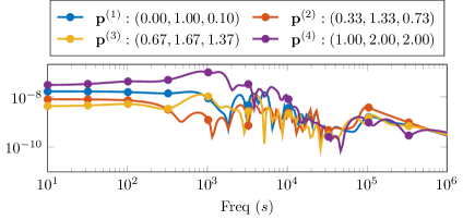
Figure 5.12: Anemometer example: The Bode plots of the absolute error between the original and the reduced-order systems for four different parameter values.

5.6 Parametric Butterfly Gyroscope

As the last example, we consider a parametric butterfly gyroscope example. The butterfly is a vibrating micro-mechanical gyro, which measures angular rates in up to three axes. It is used in inertial navigation applications. The model has mainly two parameters of interest: the rotation velocity $\theta$ around the $x$-axis and the width of bearing $d$ as shown in Figure 5.13. The system and its model reduction problem has been extensively studied in [25]. A finite element discretization leads to a parametric model for the gyroscope of the form:

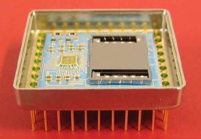
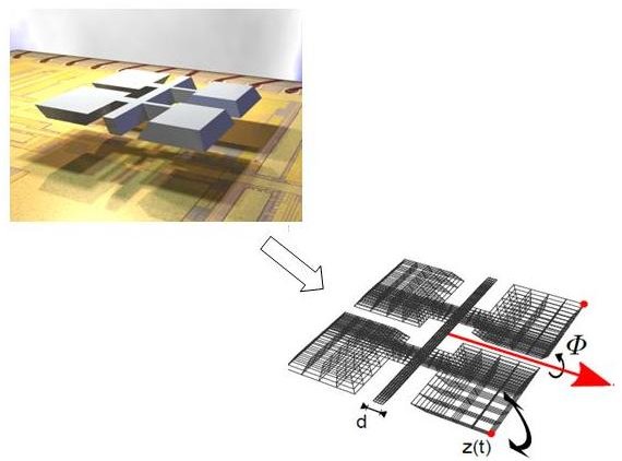
Figure 5.13: Semantic gyroscope diagram [33].

(5.7) $$\mathbf{M}(d)\ddot{}\mathbf{x}(t)+\mathbf{D}(d,\theta)\dot{}\mathbf{x}(t)+\mathbf{K}(\theta) =\mathbf{B}\mathbf{u}(t),$$

$$\mathbf{y}(t) =\mathbf{C}\mathbf{x}(t),$$

where $\mathbf{M}(d)=\mathbf{M}_{1}+d\mathbf{M}_{2}\in\mathbb{R}^{n},\mathbf{D}(d,\theta)=\theta\left(\mathbf{D}_{1}+d\mathbf{D}_{2}\right),\in\mathbb{R}^{n}$, $\mathbf{K}(d)=\mathbf{T}_{1}+\frac{1}{d}\mathbf{T}_{2}+d\mathbf{T}_{3},\in\mathbb{R}^{n}$, $\mathbf{B}\in\mathbb{R}^{n}$, and $\mathbf{C}^{T}\in\mathbb{R}^{n}$; $\mathbf{x}(t)\in\mathbb{R}^{n}$, $\mathbf{u}(t)\in\mathbb{R}^{m}$, and $\mathbf{u}(t)\in\mathbb{R}^{q}$ are the state, input and output vectors, respectively. Typical ranges for the parameters $\theta$ and $d$ are $\begin{bmatrix}10^{-5},10^{-7}\end{bmatrix}$ and $\begin{bmatrix}1,2\end{bmatrix}$, respectively. Finite-element discretization leads to $n=17,913$. Normally, the system is operated in the frequency range $2\pi\cdot\begin{bmatrix}0.025,0.25\end{bmatrix}$. For more details on the model, we refer the reader to [25, 33].

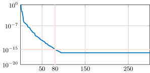
Figure 5.14: Gyro example: relative decay of the singular values obtained using Algorithm 4.1.

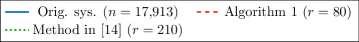
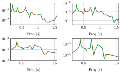
(a) The Bode plots of the original and reduced-order systems for parameter values $\mathbf{p}^{(1)}:\left(1.00,10^{-7}\right)$ at top-left, $\mathbf{p}^{(2)}:\left(1.33,4.64\cdot 10^{-7}\right)$ at top-right, $\mathbf{p}^{(3)}:\left(1.67,2.15\cdot 10^{-6}\right)$ at bottom-left and $\mathbf{p}^{(4)}:\left(2.00,10^{-5}\right)$ at top-right.

(b) The Bode plots of the absolute error between the original and reduced-order systems for the above considered parameter values.

Figure 5.15: Gyro example: Comparison of the original and reduced-order systems for different parameters values.

In order to apply the proposed method, we take $500$ points for frequency $s$ in the logarithmic way and the same number of random points for parameter $\mathbf{p}=\begin{bmatrix}d,\theta\end{bmatrix}^{T}$ in the considered range. In Figure 5.10, we first show the singular values, obtained by employing Algorithm 4.1, which indicates a rapid decay. Since the magnitude of the transfer function of the system is very small and wide range $~{}(10^{-7}{-}10^{-3})$, we choose to truncate at a relatively lower level. Hence, we truncate at $10^{-15}$, thus leading to a reduced-order system of order $r=80$. We compare the quality of the reduced-order system with the reduced-order system, obtained in [15], where the authors have obtained a reduced-order system of order $r=210$.

We compare the Bode plots of the original and reduced-order systems in Figure 5.11 for four different parameter settings and the Bode plots of the error systems are plotted in Figure 5.15. These figures indicate that both reduced-order systems are of very similar quality; but our reduced-order system is of order $r=80$, whereas the method proposed in [15] yields the reduced-order system of order $r=210$, which is more than two-and-half times larger than ours.

6 Conclusions

In this paper, we have studied model order reduction for linear structured parametric systems. Firstly, we recall the construction of an interpolatory reduced-order system for a given set of interpolation points. Then, we have defined the concepts of reachability and observability for linear structured parametric systems and connected them with the interpolation-based MOR methods. Hence, by combining both features, we discuss the construction of reduced-order systems keeping the subspaces that are the most reachable and observable simultaneously. Moreover, we have shown the efficiency of the proposed methods by means of various examples, appearing in science and engineering.

As future directions, the notion of minimal structured realizations opens several future directions, in particular, construction of minimal realization via Petrov-Galerkin projection. One interesting future direction would be to combine the knowledge of error estimates, e.g. from [15] that allows us to choose good interpolations instead of just taking them randomly or in a logarithmic scale. Moreover, an extension of structured nonlinear systems would be of highly relevant contribution to the reduced-order modeling community by combine the ideas presented in this paper and in [6].

References

- [1] B. D. O. Anderson and A. C. Antoulas, Rational interpolation and state-variable realizations, Linear Algebra Appl., 137/138 (1990), pp. 479–509.
- [2] A. C. Antoulas, Approximation of Large-Scale Dynamical Systems, SIAM Publications, Philadelphia, PA, 2005.
- [3] A. C. Antoulas, C. A. Beattie, and S. Gugercin, Interpolatory model reduction of large-scale dynamical systems, in Efficient Modeling and Control of Large-Scale Systems, J. Mohammadpour and K. M. Grigoriadis, eds., Springer US, 2010, pp. 3–58, doi:10.1007/978-1-4419-5757-3_1.
- [4] U. Baur, C. A. Beattie, P. Benner, and S. Gugercin, Interpolatory projection methods for parameterized model reduction, SIAM J. Sci. Comput., 33 (2011), pp. 2489–2518.
- [5] C. A. Beattie and S. Gugercin, Interpolatory projection methods for structure-preserving model reduction, Systems Control Lett., 58 (2009), pp. 225–232, doi:10.1016/j.sysconle.2008.10.016.
- [6] P. Benner and P. Goyal, Interpolation-based model order reduction for polynomial parametric systems, arXiv:1904.11891, 2019, https://arxiv.org/abs/1904.11891.
- [7] P. Benner, S. Gugercin, and K. Willcox, A survey of projection-based model reduction methods for parametric dynamical systems, SIAM Rev., 57 (2015), pp. 483–531, doi:10.1137/130932715.
- [8] P. Benner, V. Mehrmann, and D. C. Sorensen, Dimension Reduction of Large-Scale Systems, vol. 45 of Lect. Notes Comput. Sci. Eng., Springer-Verlag, Berlin/Heidelberg, Germany, 2005.
- [9] P. Benner and J. Saak, Efficient balancing-based MOR for large-scale second-order systems, Math. Comput. Model. Dyn. Syst., 17 (2011), pp. 123–143, doi:10.1080/13873954.2010.540822.
- [10] T. Breiten, Structure-preserving model reduction for integro-differential equations, SIAM J. Cont. Optim., 54 (2016), pp. 2992–3015, doi:10.1137/15M1032296.
- [11] Y. Chahlaoui, D. Lemonnier, A. Vandendorpe, and P. Van Dooren, Second-order balanced truncation, Linear Algebra Appl., 415 (2006), pp. 373–384, doi:10.1016/j.laa.2004.03.032.
- [12] R. F. Curtain and H. Zwart, An Introduction to Infinite-Dimensional Linear Systems Theory, vol. 21, Springer Science & Business Media, 2012.
- [13] G. E. Dullerud and F. Paganini, A Course in Robust Control Theory: a Convex Approach, vol. 36, Springer Science & Business Media, 2013.
- [14] R. Eid, B. Salimbahrami, B. Lohmann, E. B. Rudnyi, and J. G. Korvink, Parametric order reduction of proportionally damped second-order systems, Sensors and Materials, 19 (2007), pp. 149–164.
- [15] L. Feng, A. C. Antoulas, and P. Benner, Some a posteriori error bounds for reduced order modelling of (non-)parametrized linear systems, ESAIM: M2AN, (2017), doi:10.1051/m2an/2017014.
- [16] L. Feng and P. Benner, Model order reduction for systems with non-rational transfer function arising in computational electromagnetics, in Scientific Computing in Electrical Engineering SCEE 2008, J. Roos and L. R. J. Costa, eds., vol. 14 of Mathematics in Industry, Berlin/Heidelberg, 2010, Springer-Verlag, pp. 512–522.
- [17] P. A. Fuhrmann, Exact controllability and observability and realization theory in Hilbert space, J. Math. Anal. Appl., 53 (1976), pp. 377–392.
- [18] G. Gripenberg, S.-O. Londen, and O. Staffans, Volterra integral and functional equations, vol. 34, Cambridge University Press, 1990.
- [19] E. Jarlebring, T. Damm, and W. Michiels, Model reduction of time-delay systems using position balancing and delay Lyapunov equations, Math. Control Signals Systems, 25 (2013), pp. 147–166.
- [20] E. W. Kamen, Lectures on algebraic system theory: Linear systems over rings, Tech. Report NASA Contractor Report 3016, 1978.
- [21] E. W. Kamen, Linear systems over rings: From R. E. Kalman to the present, in Math. System Theory, Springer, 1991, pp. 311–324.
- [22] E. Lee and A. Olbrot, Observability and related structural results for linear hereditary systems, Internat. J. Control, 34 (1981), pp. 1061–1078.
- [23] A. J. Mayo and A. C. Antoulas, A framework for the solution of the generalized realization problem, Linear Algebra Appl., 425 (2007), pp. 634–662.
- [24] R. W. Miller, Flow measurement engineering handbook, McGraw-Hill, New York, 1996.
- [25] C. Moosmann, ParaMOR - Model Order Reduction for parameterized MEMS applications, PhD thesis, Albert-Ludwigs-Universität Freiburg, 2007, http://nbn-resolving.de/urn:nbn:de:bsz:25-opus-39719.
- [26] C. Moosmann, E. Rudnyi, A. Greiner, J. Korvink, and M. Hornung, Parameter preserving model order reduction of a flow meter, Proc. Nanotech, 3 (2005), pp. 684–687.
- [27] A. S. Morse, Ring models for delay-differential systems, Automatica, 12 (1976), pp. 529–531.
- [28] E. Plischke, Transient effects of linear dynamical systems, PhD thesis, Universität Bremen, Germany, 2005.
- [29] T. Reis and T. Stykel., Balanced truncation model reduction of second-order systems, Math. Comput. Model. Dyn. Syst., 14 (2008), pp. 391–406.
- [30] P. Schulze, B. Unger, C. Beattie, and S. Gugercin, Data-driven structured realization, Linear Algebra Appl., 537 (2018), pp. 250–286.
- [31] E. Sontag, Linear systems over commutative rings: a survey, Ricerche di Automatica, 7 (1976), pp. 1–34.
- [32] The MORwiki Community, Anemometer. MORwiki – Model Order Reduction Wiki, 2018, http://modelreduction.org/index.php/Anemometer.
- [33] The MORwiki Community, Modified gyroscope. MORwiki – Model Order Reduction Wiki, 2018, http://modelreduction.org/index.php/Modified_Gyroscope.
- [34] M. Vidyasagar, On the controllability of infinite-dimensional linear systems, J. Opt. Th. Appl., 6 (1970), pp. 171–173.
- [35] L. Weiss, On the controllability of delay-differential systems, SIAM J. Cont. Optim., 5 (1967), pp. 575–587.
- [36] S. Yi, P. W. Nelson, and A. G. Ulsoy, Controllability and observability of systems of linear delay differential equations via the matrix Lambert W function, IEEE Trans. Autom. Control, 53 (2008), pp. 854–860.