Rydberg excitons in electric and magnetic fields obtained with the complex-coordinate-rotation method

Abstract

The complete theoretical description of experimentally observed magnetoexcitons in cuprous oxide has been achieved by F. Schweiner et al[Phys. Rev. B 95, 035202 (2017)], using a complete basis set and taking into account the valence band structure and the cubic symmetry of the solid. Here, we extend these calculations by investigating numerically the autoionising resonances of cuprous oxide in electric fields and in parallel electric and magnetic fields oriented in [001] direction. To this aim we apply the complex-coordinate-rotation method. Complex resonance energies are computed by solving a non-Hermitian generalised eigenvalue problem, and absorption spectra are simulated by using relative oscillator strengths. The method allows us to investigate the influence of different electric and magnetic field strengths on the position, the lifetime, and the shape of resonances.

Keywords: Rydberg excitons, complex coordinate-rotation, electric and magnetic fields, cuprous oxide

1 Introduction

Excitons are quasi particles, which occur in semiconductors and insulators. If an electron is raised from the valence band to the conduction band, the remaining positively charged hole in the valence band interacts with the negatively charged electron in the conduction band. This electron-hole pair is called an exciton. Depending on the spatial distance between electron and hole one distinguishes between Frenkel and Mott-Wannier excitons [1, 2]. Frenkel excitons are confined to one lattice atom, whereas Mott-Wannier excitons extend over many unit cells and can be treated approximately as a hydrogenlike system.

An ideally suitable crystal for the experimental investigation of Rydberg excitons is cuprous oxide (Cu₂O), where excitons have been observed up to principal quantum number $n=25$ [3, 4]. This has opened the field of research of giant Rydberg excitons. As a consequence of the non-parabolic valence band structure of Cu₂O, the simple hydrogenlike model does not describe the exciton spectra very well [5, 6]. This is especially true for excitons in external electric or magnetic fields. Heckötter et al[7] have investigated the influence of different (weak) electric fields on the transmission spectra and have shown that the transmission spectra depend on the crystal orientation and the light polarisation. Schweiner et al[8] have calculated the absorption spectra of magnetoexcitons for various magnetic field strengths by using a complete basis set and considering the complex valence band structure. The detailed comparison between the experimental and theoretical spectra shows excellent agreement. Similar is true for exciton spectra in the Voigt configuration, where the external magnetic field is perpendicular to the incident light and a weak effective electric field perpendicular to the magnetic field is induced by the Magneto-Stark effect [9].

The experiments and calculations mentioned above are restricted to bound states, and the experimentally observed linewidths are dominated by exciton-phonon interactions [10, 11]. However, by applying an external electric field, the potential barrier of the Coulomb potential is lowered. The electron can tunnel, and former bound states become quasi-bound or resonance states. They can be described by complex energies, where the imaginary part is related to the decay rate and thus the linewidth of the resonance state.

The dissociation of excitons in Cu₂O by an electric field has been investigated by Heckötter et al[12]. It has been shown that, similar to the Stark effect in atoms, the field strength for dissociation decreases with increasing principal quantum number $n$, but increases, for fixed $n$, with growing exciton energy. The experimental results have been compared with a theoretical computation based on a simplified hydrogen-like model neglecting spin, spin-orbit, and exchange interactions.

In the present paper we want to go beyond these calculations and investigate the unbound resonance states of excitons in electric fields or combined electric and magnetic fields by fully including the effects of the valence band. To this aim we extend the method introduced in [6, 8] for the computation of exciton spectra using a complete basis set, by the method of complex coordinate-rotation [13, 14, 15], which transforms the Hermitian Hamiltonian with real eigenvalues to a non-Hermitian operator with possibly complex eigenvalues. The complex coordinate-rotation is a well established technique for the computation of resonances in atomic physics, and has already been applied, e.g., to the hydrogen atom in external fields [16, 17, 18, 19]. Here, we will calculate the positions of excitonic resonances in the complex plane. In particular, we will discuss the appearance and position of resonance states depending on the electric field strength in Faraday configuration, where the external field is parallel to the incident light. Additionally, we will investigate the behaviour of resonance states in parallel electric and magnetic fields. We are also able to calculate directly the relative oscillator strength, e.g., for $\sigma^{+}$ and $\sigma^{-}$ polarised light and to simulate the corresponding absorption spectra.

The paper is organised as follows: In section 2 we present the theory. After the introduction of resonance states and the complex coordinate-rotation-method in section 2.1 we present in section 2.2 the Hamiltonian for the yellow excitons in Cu₂O taking into account the non-parabolic valence band structure and the effects of the external electric and magnetic fields. In section 2.3 we discuss the setup of the non-Hermitian generalised eigenvalue problem by using a complete basis set. Formulas for the calculation of the relative oscillator strength and the simulation of the absorption spectra are derived in section 2.4. The results of our calculations are presented in section 3, and conclusions are drawn in section 4.

2 Theory

For the convenience of the reader we briefly recapitulate the complex-coordinate-rotation method and the Hamiltonian of cuprous oxide in external fields. We then discuss the setup of a non-Hermitian generalised eigenvalue problem for the computation of the complex resonance energies and the corresponding eigenstates, and finally present the necessary equations for the calculation of the oscillator strengths and the simulation of the absorption spectra.

2.1 Complex coordinate-rotation

Resonances are quasi-bound states with a finite lifetime. Simple examples are the radioactive decay of unstable atomic nuclei, an excited atom returning to its ground state, or a temporally trapped particle in an open potential. In the case of excitons the potential barrier of the Coulomb interaction between electron and hole can be lowered by an external electric field. To describe the temporal decay of such systems we use non-Hermitian Hamiltonians obtained with the method of the complex coordinate-rotation [13, 14, 15].

To introduce the formalism we calculate the energy expectation value of the 1S state of the hydrogen atom,

$$\braket{E}=\frac{\int_{0}^{\infty}R(r)\left[-\frac{1}{2}\frac{1}{r^{2}}\frac{\rm{d}}{\rm{d}r}r^{2}\frac{\rm{d}}{\rm{d}r}-\frac{1}{r}\right]R(r)r^{2}\rm{d}r}{\int_{0}^{\infty}R^{2}(r)r^{2}\rm{d}r}=-\frac{1}{2}$$ (1)

with radial function $R(r)=2e^{-r}$. Since $R(r)$ is an analytic function we can use Cauchy’s integral theorem and rewrite the real line integral (1) into a complex one [13],

$$\braket{E}=\frac{\int_{C}R(z)\left[-\frac{1}{2}\frac{1}{z^{2}}\frac{\rm{d}}{\rm{d}z}z^{2}\frac{\rm{d}}{\rm{d}z}-\frac{1}{z}\right]R(z)z^{2}\rm{d}z}{\int_{C}R^{2}(z)z^{2}\rm{d}z}=-\frac{1}{2}$$ (2)

with $z=re^{i\theta}$ and $\theta$ the angle between real and imaginary part. As long as we integrate from $z=0$ to $\infty$ the integral (2) does not depend on the value of $\theta$, because the wave function $R(r)$ vanishes sufficiently quickly for $r\rightarrow\infty$. Thus, the results of both integrals (1) and (2) are the same, i.e., an important property of the method is that bound states are invariant under complex rotation.

To illustrate what happens to the scattering and continuum states, we substitute $r\to re^{i\theta}$ and $k\to ke^{-i\theta}$ in the result of the radial scattering problem [15],

$$\Psi_{\mathrm{scatt}}(r)=A(k)\frac{e^{ikr}}{r}+B(k)\frac{e^{-ikr}}{r}\,.$$ (3)

The complex rotation implies a change of the energy (with $m=1$, $\hbar=1$),

$$E=\frac{1}{2}k^{2}\rightarrow E=\frac{1}{2}k^{2}e^{-2i\theta}\,,$$ (4)

which means that these states are now rotated into the lower half of the complex plane by the angle $2\theta$.

The most important feature of the complex coordinate-rotation concerns the resonance states. For appropriately chosen $\theta$, they appear as new eigenvalues on the lower half of the complex energy plane. A simple example is the inverted harmonic oscillator, which has no bound states. The complex rotated Hamiltonian is given by [13]

$$H_{\mathrm{rot}}=-\frac{1}{2}e^{-2i\theta}\frac{\rm{d}^{2}}{\rm{d}x^{2}}-\frac{1}{2}e^{2i\theta}x^{2}$$ (5)

with purely imaginary energy eigenvalues

$$E_{n}=-i\left(n+\frac{1}{2}\right)\,.$$ (6)

The inverted harmonic oscillator thus has an infinite number of resonances with different widths $\Gamma_{n}=-2\,\mathrm{Im}\,E_{n}=2n+1$.

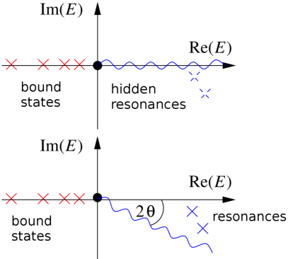
Figure 1: Effect of the complex coordinate-rotation. The hidden resonances are exposed by the rotation of the continuum states.

The results of the complex rotation can be summarised by the following statements, which are also illustrated in figure 1: (i) The real-valued bound states are invariant under the complex rotation. (ii) The energy values of the scattering respectively continuum states are rotated into the lower half of the complex plane by $2\theta$. (iii) For appropriately chosen angles $\theta$ resonances are exposed by the rotation of the continuum states.

2.2 Hamiltonian of yellow excitons in external fields

For the calculation of the yellow exciton series in Cu₂O we use the same Hamiltonian as Schweiner et al[6, 8, 20]. Without external fields the Hamiltonian can be written as

$$H=E_{\rm g}+H_{e}(\bi{p}_{\rm e})+H_{\rm h}(\bi{p}_{\rm h})+V(\bi{r}_{\rm h}-\bi{r}_{\rm e})\,,$$ (7)

where the kinetic energy of the electron and hole are given by

$$H_{e}(\bi{p}_{\rm e}) =\frac{\bi{p}_{\rm e}^{2}}{2m_{\rm e}}\,,$$ (8)

$$H_{\rm h}(\bi{p}_{\rm h}) =H_{\rm SO}+\frac{1}{2\hbar^{2}m_{0}}\{\hbar^{2}(\gamma_{1}+4\gamma_{2})\bi{p}^{2}_{\rm h}$$ (9)

$$+2(\eta_{1}+2\eta_{2})\bi{p}^{2}_{\rm h}(\bi{I}\cdot\bi{S}_{\rm h})$$

$$-6\gamma_{2}(p^{2}_{\rm h1}\bi{I}^{2}_{1}+{\rm c.p.})$$

$$-12\eta_{2}(p^{2}_{\rm h1}\bi{I}_{1}\bi{S}_{\rm h1}+{\rm c.p.})$$

$$-12\gamma_{3}(\{p_{\rm h1},p_{\rm h2}\}\{\bi{I}_{1},\bi{I}_{2}\}+{\rm c.p.})$$

$$-12\eta_{3}(\{p_{\rm h1},p_{\rm h2}\}(\bi{I}_{1}\bi{S}_{\rm h2}+\bi{I}_{2}\bi{S}_{\rm h1})+{\rm c.p.})\}\,,$$

with the spin-orbit interaction

$$H_{\rm SO}=\frac{2}{3}\Delta\left(1+\frac{1}{\hbar^{2}}\bi{I}\cdot\bi{S}_{\rm h}\right).$$ (10)

Here, $E_{\mathrm{g}}$ is the gap energy, $m_{\rm e}$ is the effective electron mass, $\bi{p}=(p_{1},p_{2},p_{3})$ are the momenta, $\{a,b\}=\frac{1}{2}(ab+ba)$ is the symmetric product, $\Delta$ is the spin-orbit coupling constant, $\bi{I}$ is the quasispin, $\bi{S}_{\rm h}$ is the hole spin, and c.p. denotes cyclic permutation. The vectors $\bi{I}$ and $\bi{S}_{\rm h}$ contain the components of the three spin matrices $\bi{S}_{\rm{h}j}$ and $\bi{I}_{j}$ of the hole spin $S_{\rm h}=1/2$ and the quasispin $I=1$, respectively. The quasispin $\bi{I}$ is introduced to describe the degeneracy of the valence band Bloch functions [21]. The corresponding matrices fulfil the commutation relations of a spin $I=1$. The parameters $\eta_{j}$ and the three Luttinger parameters $\gamma_{j}$ are used to describe the behaviour and the anisotropic effective hole mass in the vicinity of the $\Gamma$ point [6]. The electric interaction between hole and electron is given by the Coulomb potential

$$V(\bi{r}_{\rm h}-\bi{r}_{\rm e})=-\frac{e^{2}}{4\pi\epsilon_{0}\epsilon|\bi{r}_{\rm h}-\bi{r}_{\rm e}|}$$ (11)

with the dielectric constant $\epsilon$. In references [20, 22] additional central cell corrections were included in the Hamiltonian. Since these effects are only important for states with principal quantum numbers $n\leq 2$ [20], which we do not consider in this paper, these corrections can be neglected here.

To take external electric and magnetic fields into account the Hamiltonian (7) must be extended. The electric field is included by adding the potential

$$V_{\rm F}(\bi{r}_{\rm h}-\bi{r}_{\rm e})=-e(\bi{r}_{\rm h}-\bi{r}_{\rm e})\cdot\bi{F}\,,$$ (12)

where $\bi{F}$ is the electric field vector. To describe a constant magnetic field we use the vector potential with symmetric gauge, $\bi{A}=(\bi{B}\times\bi{r})/2$. The energy of the spins in the magnetic field is given by

$$H_{\rm B}=\mu_{\rm B}\left[g_{\rm c}\bi{S}_{\rm e}+(3\kappa+g_{\rm s}/2)\bi{I}-g_{\rm s}\bi{S}_{\rm h}\right]\cdot\bi{B}/\hbar\,,$$ (13)

with $\mu_{\rm B}$ the Bohr magneton, $g_{\rm s}$ the g factor of the hole spin $\bi{S}_{\rm h}$, $g_{\rm c}$ the g factor of the electron spin $\bi{S}_{\rm e}$, and $\kappa$ the fourth Luttinger parameter, which has been determined by Schweiner et al[8]. Next we introduce relative and centre of mass coordinates [23],

$$\bi{r} =\bi{r}_{\rm h}-\bi{r}_{\rm e}\,,\quad\bi{R}=\frac{m_{\rm h}\bi{r}_{\rm h}+m_{\rm e}\bi{r}_{\rm e}}{m_{\rm h}+m_{\rm e}}\,,$$

$$\bi{P} =\bi{p}_{\rm h}+\bi{p}_{\rm e}\,,\quad\bi{p}=\frac{m_{\rm h}\bi{p}_{\rm e}-m_{\rm e}\bi{p}_{\rm h}}{m_{\rm h}+m_{\rm e}}\,,$$ (14)

and set the position and momentum of the centre of mass to zero ($\bi{R}=0$, $\bi{P}=0$). The complete Hamiltonian of excitons in external fields with relative coordinates finally reads

$$H =E_{\rm g}+H_{e}(\bi{p}+e\bi{A}(\bi{r}))+H_{\rm h}(-\bi{p}+e\bi{A}(\bi{r}))$$ (15)

$$+V(\bi{r})+H_{\rm B}+V_{\rm F}(\bi{r})\,.$$

More details of the derivations are given in references [6, 8, 22]. The material parameters for Cu₂O used in our calculations are listed in table 1.

Table 1: Material parameters of Cu₂O used in the calculations.

Energy gap	$E_{\rm g}=2.17208\,$eV	[7]
Effective electron mass	$m_{\rm e}=0.99m_{0}$	[24]
Effective hole mass	$m_{\rm h}=0.58m_{0}$	[24]
Dielectric constant	$\epsilon=7.5$	[25]
Spin-orbit coupling	$\Delta=0.131\,$eV	[5]
Valence band parameter	$\gamma_{1}=1.76$	[5]
	$\gamma_{2}=0.7532$	[5]
	$\gamma_{3}=-0.3668$	[5]
	$\kappa=-0.5$	[8]
	$\eta_{1}=-0.020$	[5]
	$\eta_{2}=-0.0037$	[5]
	$\eta_{3}=-0.0337$	[5]
g factor of the electron spin	$g_{\rm c}=2.1$	[8]
g factor of the hole spin	$g_{\rm s}\approx 2$	[8]

2.3 Non-Hermitian generalised eigenvalue problem

For the computation of eigenvalues of the yellow excitons in external fields we now express the Hamiltonian (15) as a matrix by using an appropriate basis set. For the radial part of the wave functions we use the Coulomb-Sturmian functions [26]

$$U_{NL}(\rho)=N_{NL}(2\rho)^{L}e^{-\rho}L_{N}^{2L+1}(2\rho)\,,$$ (16)

where $L_{N}^{2L+1}$ are the associated Laguerre polynomials, the $N_{NL}$ are normalisation factors, and $\rho=r/\alpha$, with $\alpha$ being a free parameter. $N$ is the radial quantum number, which is related to the principal quantum number $n$ via $n=N+L+1$. Note that the Coulomb-Sturmian functions (16) form a complete basis, however, they are not orthogonal. For the computation of resonances the complex coordinate-rotation $r\to r\rme^{\rmi\theta}$ discussed in section 2.1 is equivalent to choosing the free parameter $\alpha$ as being complex, i.e., $\alpha=|\alpha|\rme^{\rmi\theta}$.

For the angular part of the basis we use the eigenfunctions of the effective hole spin $J=I+S_{\rm h}$, the effective angular momentum $F=L+J$, and the electron spin $S_{\rm e}$. At the $\Gamma$ point, $J$ is a good quantum number and distinguishes between the yellow exciton series ($J=1/2$) and the green exciton series ($J=3/2$). $F$ and $S_{\rm e}$ are coupled to $F_{t}=F+S_{\rm e}$ with $z$ component $M_{F_{t}}$. The complete basis set is then given by [6, 8]

$$\ket{\Pi}=\ket{N,L;(I,S_{h}),J;F,S_{e};F_{t},M_{F}}\,.$$ (17)

To obtain a finite size basis for the numerical computations the quantum numbers must be restricted. For each value of the principal quantum number $n=N+L+1$ we use [6]

$$L =0,\dots,n-1,$$

$$J =1/2,3/2,$$

$$F =|L-J|,\dots,\min(L+J,F_{\max}),$$

$$F_{t} =F-1/2,F+1/2,$$

$$M_{F_{t}} =-F_{t},\dots,F_{t}\,.$$ (18)

The excitonic wave functions can be expanded in the basis (17) as

$$\ket{\Psi}=\sum_{NLJFF_{t}M_{F_{t}}}c_{NLJFF_{t}M_{F_{t}}}\ket{\Pi}\,,$$ (19)

with the coefficients $\bi{c}$. Using the Hamiltonian (15) and the basis set (17) we can now set up the generalised eigenvalue problem

$$\bi{Dc}=E\bi{Mc}$$ (20)

for the resonance energies $E$ and the coefficients $\bi{c}$ of the corresponding wave functions (19). The matrix elements of the matrices $\bi{D}$ and $\bi{M}$ are given in the appendices of references [6, 8] with the only difference that $\alpha$ is now a complex parameter $\alpha=|\alpha|\rme^{\rmi\theta}$ with $\theta$ the angle of the complex coordinate-rotation, as explained above. The matrix $\bi{M}$ in (20) is the overlap matrix of the basis states (17) and differs from the identity matrix because, as mentioned, the Coulomb-Sturmian functions (16) are not orthogonal.

Note that both matrices $\bi{D}$ and $\bi{M}$ in (20) are complex symmetric but non-Hermitian matrices. The generalised eigenvalue problem (20) can be solved numerically by application of the QZ algorithm, which is implemented in the LAPACK routine ZGGEV [27]. To achieve convergence of the eigenvalues and eigenvectors the maximum value for $n$ and the value $F_{\max}$ for the setup (18) of the basis must be chosen sufficiently large. The LAPACK routine does not provide normalised eigenvectors. For the computation of oscillator strengths in the next section 2.4 the wave functions (19) must be normalised according to

$$\braket{\Psi_{i}}{\bi{M}}{\Psi_{j}}=\delta_{ij}\,,$$ (21)

which is achieved with a modified Gram-Schmidt process.

2.4 Oscillator strengths

With the eigenvalues and eigenvectors obtained by numerical diagonalisation of the generalised eigenvalue problem (20) we are able to calculate the oscillator strengths for dipole transitions. Note that the crystal ground state depends on Bloch functions, which are not explicitly known, and therefore only relative oscillator strengths can be computed [22]. For circularly polarised light the relative oscillator strength is given by [8]

$$f_{\rm{rel}}\sim\left(\lim_{r\rightarrow 0}{\frac{\partial}{\partial r}\braket{\sigma^{\pm}_{z}}{\Psi(\bi{r})}}\right)^{2}$$ (22)

with

$$\ket{\sigma^{+}_{z}}=\frac{-i}{\sqrt{2}}\left(\ket{\pi_{x}}+i\ket{\pi_{y}}\right)=\ket{2,-1}_{D},$$ (23)

$$\ket{\sigma^{-}_{z}}=\frac{i}{\sqrt{2}}\left(\ket{\pi_{x}}-i\ket{\pi_{y}}\right)=-\ket{2,1}_{D},$$ (24)

and

$$\ket{\pi_{x}}=\frac{i}{\sqrt{2}}\left(\ket{2,-1}_{D}+\ket{2,1}_{D}\right),$$ (25)

$$\ket{\pi_{y}}=\frac{1}{\sqrt{2}}\left(\ket{2,-1}_{D}+\ket{2,1}_{D}\right),$$ (26)

for an electric and/or magnetic field in $[001]$ direction. We use the abbreviation $\ket{F_{t},M_{F_{t}}}_{D}$ to denote the states

$$\ket{F_{t},M_{F_{t}}}_{D} =\ket{(S_{\rm e},S_{\rm h})\,S,\,I;\,I+S,\,L;\,F_{t},\,M_{F_{t}}}$$ (27)

$$=\ket{(1/2,1/2)\,0,\,1;\,1,\,1;\,F_{t},\,M_{F_{t}}}\,,$$

where the coupling scheme differs from the one given in section 2.3. The spins couple in the following way [8]:

$$S_{\rm e}+S_{\rm h}=S\rightarrow(I+S)+L=F_{t}\,,$$ (28)

with the total spin $S$, the quasispin $I$, the angular momentum $L$, the total angular momentum $F_{t}$ and its projection on the quantisation axis $M_{F_{t}}$. With the relative oscillator strength we can furthermore calculate the spectrum. Rescigno and McKoy [28] have shown that the photoabsorption cross section in atomic physics, using the complex coordinate-rotation, can be written as

$$\sigma(E)=4\pi\alpha(E-E_{0})\,\mathrm{Im}\sum_{j}\frac{\braket{\Psi_{0}}{D}{\Psi_{j}(\theta)}^{2}}{E_{j}-E},$$ (29)

where $\alpha$ is the fine-structure constant, $E_{0}$ the energy of the ground state $\Psi_{0}$, and $E_{j}$ the complex energy of the resonance state $\Psi_{j}$. For excitonic spectra we replace the squared dipole matrix elements $\braket{\Psi_{0}}{D}{\Psi_{j}(\theta)}^{2}$ in (29) with the relative oscillator strengths $f_{\mathrm{rel}}$ given in (22). The excitonic absorption spectrum then reads

$$f(E)=-\frac{1}{\pi}{\mathrm{Im}}\sum_{j}\frac{f_{\rm rel}^{(j)}}{E-E_{j}}$$ (30)

with $E_{j}$ the complex energies of the resonances. Note that the squared dipole matrix elements $\braket{\Psi_{0}}{D}{\Psi_{j}(\theta)}^{2}$ in (29) and the relative oscillator strength $f_{\mathrm{rel}}$ in (22) are real-valued for bound states but can become complex for resonances, because, after complex coordinate-rotation, bra vectors are not the complex conjugate of the ket vectors (see [13, 14, 15]), as in Hermitian quantum mechanics. The complex phases of $f_{\mathrm{rel}}$ lead to deviations of resonance shapes from a Lorentzian profile in (30).

3 Results and discussion

In this section we present the results of our calculations for excitons of cuprous oxide in external fields. We investigate the resonances in the complex energy plane and the corresponding absorption spectra obtained with circularly polarised light for excitons, first in electric fields, and then in parallel electric and magnetic fields. We restrict the presentation of results to resonances and ignore the bound states, which would appear as delta peaks in the absorption spectra. The linewidths of resonances in our calculations are solely caused by the external electric field, i.e., we do not consider exciton-phonon interactions [10, 11].

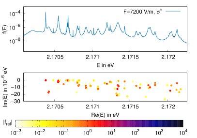
Figure 2: Lower part: Positions of resonances in the complex energy plane for excitons in cuprous oxide in an electric field with field strength $F=7200\,$V/m in [001] direction. The colours of the symbols encode the absolute values of the relative oscillator strengths $f_{\mathrm{rel}}$ for excitations with $\sigma^{\pm}$ polarised light. Upper part: The corresponding absorption spectra for excitations with $\sigma^{+}$ and $\sigma^{-}$ polarised light coincide.

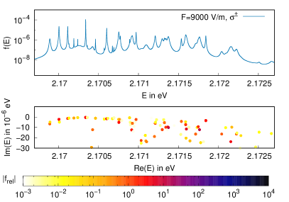
Figure 3: Same as figure 2 but for $F=9000\,$V/m.

3.1 Electric fields in [001] direction

In figures 2 and 3 we present the results for excitons in an electric field oriented along the [001] axis with field strengths $F=7200\,$V/m and $F=9000\,$V/m, respectively. The lower parts of the figures show the positions of resonances in the complex energy plane obtained as complex eigenvalues of the non-Hermitian generalised eigenvalue problem (20). For the computations we used the basis (17) with principal quantum numbers up to $n=30$ and $F_{\max}=15$ resulting in a total set of $5303$ basis functions. For the complex coordinate-rotation we used rotation angles in the region $0.1<\theta<0.3$. The colours of the resonance positions encode the absolute values of the relative oscillator strengths $f_{\mathrm{rel}}$ for excitations with circularly polarised light given by (22). The upper parts of figures 2 and 3 show the absorption spectra $f(E)$ obtained using (30). Note that the absorption spectra for $\sigma^{+}$ and $\sigma^{-}$ polarised light coincide as expected.

The spectrum at $F=7200\,$V/m, in figure 2, exhibits resonances with quite different linewidths. Long-lived resonances appear as thin peaks in the absorption spectra. In general, broader peaks belong to resonances with higher principal quantum numbers $n$ or, within a given $n$-manifold, to resonances with lower energy [12]. The resonances shown in the figure belong to principal quantum numbers between $n=8$ and $n=15$. Note that, for the chosen electric field strength, the different $n$-manifolds already strongly overlap. If we increase the electric field strength to $F=9000\,$V/m, new long-lived resonance states appear (see figure 3) and the lifetimes of the resonances with higher real energy part decrease. If we compare the positions in both plots, we recognise that more resonances appear deeper in the lower half of the complex energy plane. Undoubtedly, the reason for this is the electric field which lowers the potential barrier of the Coulomb potential and therefore increases the tunnel probability.

Figure 4 shows the absorption spectra for different electric field strengths from $F=3400\,$V/m to $F=21600\,$V/m. The single spectra $f(E)$ are plotted with an offset, therefore no units of $f$ are given. For the computations we have used the same basis set as described above. The figure shows the evolution of the spectra in dependence on the electric field strength. All spectra are restricted to the range where resonances appear. At lower energies only bound states would appear and at higher ones the spectra would show unconverged states due to the finite basis.

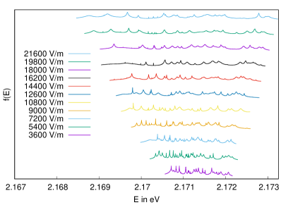
Figure 4: Evolution of resonance spectra for $\sigma^{\pm}$ polarised light as a function of the electric field. The electric field strength increases from $F=3600\,$V/m (bottom) to $F=21600\,$V/m (top), and is orientated in the [001] direction.

We first notice the fan-like spreading of the absorption spectra. That means for $F=3600\,$V/m we found resonances between $2.17056\,$eV and $2.17216\,$eV and for $F=21600\,$V/m we found resonances between $2.16846\,$eV and $2.17324\,$eV. This behaviour derives from the Stark effect which splits the energy levels and moves the positions of the resonances along the real axis. Additionally, the decrease of the potential barrier moves the resonances deeper into the lower half of the complex plane. Therefore we observe mostly resonances with short lifetime (broad peaks) for field strengths $F>14400\,$V/m. New lines always appear as sharp peaks (long-lived resonances) on the left hand side of the absorption spectra. For higher field strengths the number of exposed resonances decreases because the maximum value of $\theta$ is too small. In principle, we could increase $\theta$ to uncover these states, however, in that case the basis set must be increased, which leads to higher computation times.

In reference [12] it has been shown that the field strength for the dissociation of excitons in Cu₂O decreases with increasing principal quantum number $n$, but increases, for fixed $n$, with growing exciton energy, in agreement with similar results for the Stark effect in atoms. We expect a similar behaviour in our spectra, however, this can not easily be observed because we are in an energy and field strength region, where states with different $n$ strongly overlap. In particular, we have not yet been able to assign any (approximate) quantum numbers to the resonances shown in figure 4. To do so, e.g. the evolution of resonance spectra in figure 4 must be followed on a much denser grid of field strengths down to the field-free spectrum. As the computation of each spectrum is numerically very expensive this is currently beyond our numerical capabilities.

3.2 Parallel electric and magnetic fields

Now we investigate the influence of an additional magnetic field parallel to the electric field. Both fields are in [001] direction.

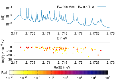
Figure 5: Position and resonance spectra for an electric field $F=7200\,$V/m and magnetic field $B=0.5$ T. Both fields are in [001] direction and the light is $\sigma^{-}$ polarised.

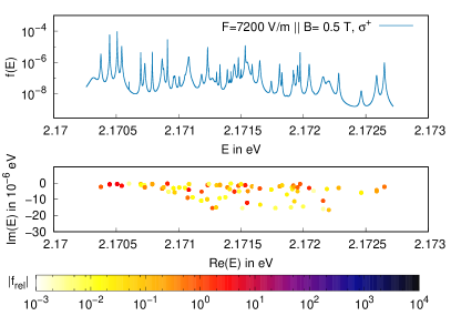
Figure 6: Same as figure 5 but for $\sigma^{+}$ polarised light.

Figure 5 shows the positions of the resonances in the complex energy plane and the absorption spectrum for $F=7200\,$V/m, $B=0.5\,$T and $\sigma^{-}$ polarised light. For the same field strength but with $\sigma^{+}$ polarised light, figure 6 shows the absorption spectrum and the positions of resonances in the complex energy plane. As discussed above, both spectra consist of long-lived resonances, thin peaks, and short-lived ones, broad peaks, but if we compare the spectra of $\sigma^{-}$ and $\sigma^{+}$ polarised light (see figure 6) they differ from each other. This is due to the magnetic field and the symmetry of the valence band. In [8] it is shown that different excitons are excited by $\sigma^{-}$ and $\sigma^{+}$ polarised light with a magnetic field in [001] direction. With $\sigma^{+}$ polarised light excitons with a large amount of angular momentum $L=1$, $F_{t}=2$, $M_{F_{t}}=-1$ and with $\sigma^{-}$ polarised light excitons with a large amount of angular momentum $L=1$, $F_{t}=2$, $M_{F_{t}}=+1$ (cf. equations (23) and (24)) are strongly excited. These states are non-degenerate in a magnetic field or in parallel magnetic and electric fields. We note that, as for the Stark spectra discussed above, we are not able to assign any quantum numbers to individual resonances.

4 Conclusion and outlook

Schweiner et al[6, 8] have developed a method for the numerically exact computation of yellow excitons in cuprous oxide by using a complete basis set. We have extended and augmented this technique by application of the complex-coordinate-rotation method, which, as a novel result, allows for the computation of unbound excitonic resonance states. We have used the method to calculate the positions of resonances in the complex energy plane, and thus the decay rates, for excitons in external electric fields and in parallel electric and magnetic fields. Furthermore, we have simulated the absorption spectra for excitations with circularly polarised light, and have shown that the spectra obtained with $\sigma^{+}$ and $\sigma^{-}$ polarised light coincide for excitons in an electric field but significantly differ for excitons in combined electric and magnetic fields.

The computation of magnetoexcitons including the effects of the valence band have allowed for detailed line-by-line comparisons between experimental and theoretical spectra [8]. A detailed comparison of our theoretical excitonic resonances with experimental absorption spectra [12] will be an interesting future task and will clarify the validity or limitations of the hydrogenlike model, with its refinements.

An interesting property of the complex generalised eigenvalue problem (20) is that for certain values of the electric and magnetic field strengths the resonance energies and also the corresponding eigenstates can become degenerate. This situation is not possible in Hermitian quantum mechanics, and is called an exceptional point [29, 30, 31]. Such points have been found in computations for the hydrogen atom in combined electric and magnetic fields, however, at very high and thus experimentally not accessible field strengths [18, 19, 32]. With the method introduced in this paper it will be possible to search for exceptional points in the spectra of cuprous oxide and in regions of the field strengths, which can easily be realised in experiments. Cuprous oxide could therefore be an excellent candidate for the first experimental observation of an exceptional point in a Rydberg system.

Nikitine [33] has investigated experimentally the green exciton series in Cu₂O and, recently, Krüger and Scheel [34] have focused on the interseries transitions, e.g., between yellow and green excitons. In this context, a better understanding of the green exciton series is desirable. Since the green series is located inside of the yellow continuum [35, 36, 37], and the different series couple, the green exciton states are actually resonances. The complex coordinate-rotation method used in this paper thus is also an appropriate tool for the future investigation of these resonance states.

References

References

- [1] N. F. Mott. Conduction in polar crystals. ii. the conduction band and ultra-violet absorption of alkali-halide crystals. Trans. Faraday Soc., 34:500–506, 1938.
- [2] Gregory H. Wannier. The structure of electronic excitation levels in insulating crystals. Phys. Rev., 52:191–197, Aug 1937.
- [3] T. Kazimierczuk, D. Fröhlich, S. Scheel, H. Stolz, and M. Bayer. Giant Rydberg excitons in the copper oxide Cu2O. Nature, 514:343, oct 2014.
- [4] J. Thewes, J. Heckötter, T. Kazimierczuk, M. Aßmann, D. Fröhlich, M. Bayer, M. A. Semina, and M. M. Glazov. Observation of high angular momentum excitons in cuprous oxide. Phys. Rev. Lett., 115:027402, Jul 2015.
- [5] F. Schöne, S.-O. Krüger, P. Grünwald, H. Stolz, S. Scheel, M. Aßmann, J. Heckötter, J. Thewes, D. Fröhlich, and M. Bayer. Deviations of the exciton level spectrum in from the hydrogen series. Phys. Rev. B, 93:075203, Feb 2016.
- [6] Frank Schweiner, Jörg Main, Matthias Feldmaier, Günter Wunner, and Christoph Uihlein. Impact of the valence band structure of on excitonic spectra. Phys. Rev. B, 93:195203, May 2016.
- [7] J. Heckötter, M. Freitag, D. Fröhlich, M. Aßmann, M. Bayer, M. A. Semina, and M. M. Glazov. High-resolution study of the yellow excitons in subject to an electric field. Phys. Rev. B, 95:035210, Jan 2017.
- [8] Frank Schweiner, Jörg Main, Günter Wunner, Marcel Freitag, Julian Heckötter, Christoph Uihlein, Marc Aßmann, Dietmar Fröhlich, and Manfred Bayer. Magnetoexcitons in cuprous oxide. Phys. Rev. B, 95:035202, Jan 2017.
- [9] Patric Rommel, Frank Schweiner, Jörg Main, Julian Heckötter, Marcel Freitag, Dietmar Fröhlich, Kevin Lehninger, Marc Aßmann, and Manfred Bayer. Magneto-stark effect of yellow excitons in cuprous oxide. Phys. Rev. B, 98:085206, Aug 2018.
- [10] Frank Schweiner, Jörg Main, and Günter Wunner. Linewidths in excitonic absorption spectra of cuprous oxide. Phys. Rev. B, 93:085203, Feb 2016.
- [11] Heinrich Stolz, Florian Schöne, and Dirk Semkat. Interaction of Rydberg excitons in cuprous oxide with phonons and photons: optical linewidth and polariton effect. New J. Phys., 20:023019, 2018.
- [12] J. Heckötter, M. Freitag, D. Fröhlich, M. Aßmann, M. Bayer, M. A. Semina, and M. M. Glazov. Dissociation of excitons in by an electric field. Phys. Rev. B, 98:035150, Jul 2018.
- [13] W. P. Reinhardt. Complex coordinates in the theory of atomic and molecular structure and dynamics. Annual Review of Physical Chemistry, 33(1):223–255, 1982.
- [14] Y. K. Ho. The method of complex coordinate rotation and its applications to atomic collision processes. Phys. Rep., 99:1–68, 1983.
- [15] Nimrod Moiseyev. Quantum theory of resonances: Calculating energies, widths and cross-sections by complex scaling. Phys. Rep., 302:211–293, 1998.
- [16] Jörg Main and Günter Wunner. Ericson fluctuations in the chaotic ionization of the hydrogen atom in crossed magnetic and electric fields. Phys. Rev. Lett., 69:586–589, Jul 1992.
- [17] Jörg Main and Günter Wunner. Rydberg atoms in external fields as an example of open quantum systems with classical chaos. J. Phys. B, 27:2835, 1994.
- [18] Holger Cartarius, Jörg Main, and Günter Wunner. Exceptional points in atomic spectra. Phys. Rev. Lett., 99:173003, Oct 2007.
- [19] Holger Cartarius, Jörg Main, and Günter Wunner. Exceptional points in the spectra of atoms in external fields. Phys. Rev. A, 79:053408, May 2009.
- [20] Frank Schweiner, Jörg Main, Günter Wunner, and Christoph Uihlein. Even exciton series in . Phys. Rev. B, 95:195201, May 2017.
- [21] J. M. Luttinger. Quantum theory of cyclotron resonance in semiconductors: General theory. Phys. Rev., 102:1030–1041, May 1956.
- [22] Frank Schweiner, Jan Ertl, Jörg Main, Günter Wunner, and Christoph Uihlein. Exciton-polaritons in cuprous oxide: Theory and comparison with experiment. Phys. Rev. B, 96:245202, Dec 2017.
- [23] P. Schmelcher and L. S. Cederbaum. Regularity and chaos in the center of mass motion of the hydrogen atom in a magnetic field. Zeitschrift für Physik D Atoms, Molecules and Clusters, 24(4):311–323, Dec 1992.
- [24] J. W. Hodby, T. E. Jenkins, C. Schwab, H. Tamura, and D. Trivich. Cyclotron resonance of electrons and of holes in cuprous oxide, Cu2O. Journal of Physics C: Solid State Physics, 9(8):1429–1439, Apr 1976.
- [25] H. Landolt, R. Börnstein, H. Fischer, O. Madelung, and G. Deuschle. Landolt-Bornstein: Numerical Data and Functional Relationships in Science and Technology. Number Bd. 17 in Numerical Data and Functional Relationships in Science and Technology Series. Springer, 1987.
- [26] M. A. Caprio, P. Maris, and J. P. Vary. Coulomb-Sturmian basis for the nuclear many-body problem. Phys. Rev. C, 86:034312, Sep 2012.
- [27] E. Anderson, Z. Bai, C. Bischof, L. S. Blackford, J. Demmel, Jack J. Dongarra, J. Du Croz, S. Hammarling, A. Greenbaum, A. McKenney, and D. Sorensen. LAPACK Users’ Guide (Third Ed.). Society for Industrial and Applied Mathematics, Philadelphia, PA, USA, 1999.
- [28] Thomas N. Rescigno and Vincent McKoy. Rigorous method for computing photoabsorption cross sections from a basis-set expansion. Phys. Rev. A, 12:522–525, Aug 1975.
- [29] T. Kato. Perturbation theory of linear operators. Springer, Berlin, 1966.
- [30] W. D. Heiss and A. L. Sannino. Avoided level crossings and exceptional points. J. Phys. A, 23:1167 – 1178, 1990.
- [31] Nimrod Moiseyev. Non-Hermitian Quantum Mechanics. Cambridge University Press, Cambridge, 2011.
- [32] Matthias Feldmaier, Jörg Main, Frank Schweiner, Holger Cartarius, and Günter Wunner. Rydberg systems in parallel electric and magnetic fields: an improved method for finding exceptional points. Journal of Physics B: Atomic, Molecular and Optical Physics, 49(14):144002, 2016.
- [33] S. Nikitine. Experimental investigations of exciton spectra in ionic crystals. The Philosophical Magazine: A Journal of Theoretical Experimental and Applied Physics, 4(37):1–31, 1959.
- [34] Sjard Ole Krüger and Stefan Scheel. Interseries transitions between Rydberg excitons in Cu2O. Phys. Rev. B, 100:085201, 2019.
- [35] J.B. Grun, M. Sieskind, and S. Nikitine. Détermination de l’intensité d’oscillateur des raies de la série verte de Cu2O aux basses températures. Journal de Physique, 22:176, 1961.
- [36] J.B. Grun and S. Nikitine. Étude de la forme des raies des séries jaune et verte de la cuprite. Journal de Physique, 24:355, 1963.
- [37] Claudia Malerba, Francesco Biccari, Cristy Leonor Azanza Ricardo, Mirco D’Incau, Paolo Scardi, and Alberto Mittiga. Absorption coefficient of bulk and thin film Cu2O. Solar Energy Materials and Solar Cells, 95(10):2848 – 2854, 2011.