A Statistical Learning Approach to Reactive Power
Control in Distribution Systems

Abstract

Pronounced variability due to the growth of renewable energy sources, flexible loads, and distributed generation is challenging residential distribution systems. This context, motivates well fast, efficient, and robust reactive power control. Real-time optimal reactive power control is possible in theory by solving a non-convex optimization problem based on the exact model of distribution flow. However, lack of high-precision instrumentation and reliable communications, as well as the heavy computational burden of non-convex optimization solvers render computing and implementing the optimal control challenging in practice. Taking a statistical learning viewpoint, the input-output relationship between each grid state and the corresponding optimal reactive power control is parameterized in the present work by a deep neural network, whose unknown weights are learned offline by minimizing the power loss over a number of historical and simulated training pairs. In the inference phase, one just feeds the real-time state vector into the learned neural network to obtain the ‘optimal’ reactive power control with only several matrix-vector multiplications. The merits of this novel statistical learning approach are computational efficiency as well as robustness to random input perturbations. Numerical tests on a $47$-bus distribution network using real data corroborate these practical merits.

I INTRODUCTION

Reliability and operational efficiency of modern distribution systems are currently being challenged by high penetration of unpredictable renewable energy resources, large-scale deployment of electric vehicles, and ‘human-in-the-loop’ demand response programs. As a consequence, reverse power flow as well as voltage magnitude fluctuations are prevailing in nowadays residential grids [4]. For instance, solar power generation may drop by $15\%$ of the photo voltaic (PV) nameplate rating within one minute due, for example, to intermittent cloud coverage [3], which will result in a sizable voltage sag if no action is taken. The role of networked control in power systems is to maintain desired operations, while preventing contingency events involving voltage and/or frequency instabilities from developing into large-scale cascades and blackouts. To protect electrical devices, bus voltage magnitudes in distribution grids are typically regulated to be within a certain range, e.g., $\pm 5\%$ around their nominal values. A common practice to achieve this is through reactive power compensation.

Traditional approaches have relied on utility-owned devices including load-tap-changing transformers, voltage regulators, and capacitor banks to control reactive power injection into the grid. Although these devices perform well in certain cases, slow response times, discrete control actions, and lifespan limitations discourage them from fast reactive power control [6]. Recent advances in smart inverters offer new opportunities by circumventing these limitations. Despite their advantages, computing the optimal setpoints for smart inverters can be cast as an instance of the optimal power flow task, which entails solving a non-convex optimization problem [6, 11]. Furthermore, to deal with the renewable energy uncertainties as well as unreliable communication links (which cause delay and even communication failures), stochastic, online, decentralized, and localized smart inverter control schemes have been developed [11, 16, 13, 23, 21]. Nonetheless, centralized solvers suffer from high computational complexity, and decentralized and localized schemes algorithms converge slowly.

To bypass these hurdles, recent proposals have engaged machine learning approaches for fast networked control and monitoring [14, 17, 20, 19, 18]. A support vector machine-based method was devised in [10] to approximate a near-optimal inverter control rule. In [17], the authors developed a voltage regulation scheme using deep reinforcement learning. Deep (recurrent) neural networks were used for power system state estimation and forecasting in [20]. By exploiting the power grid topology, a physics-aware neural network was proposed for state estimation [19]. Related schemes leveraging deep neural networks that ‘learn-to-optimize’ also appeared in resource allocation [12] and outage detection [22]. Unfortunately, training existing supervised learning models for reactive power control, requires large-scale labeled training data, which are difficult to be obtained in real-world physical systems. Reinforcement learning approaches on the other hand, entail prior knowledge on designing the so-called reward functions and often converge slowly.

Different from existing efforts, in this work an unsupervised statistical learning approach is developed for computationally intensive and time-sensitive reactive power control. Specifically, a deep neural network is used to parameterize the functional relationship between the grid state vector and the optimal reactive power compensation. The computational complexity of solving non-convex optimization problems is shifted to offline training of a deep neural network. In the training phase, by feeding grid state vectors obtained from historical data or through simulations, the weight parameters of the deep neural network are updated iteratively via policy gradient method. In the online inference phase, or real-time implementation, one just needs to pass the observed state vector into the trained deep neural network, and obtains a near-optimal reactive power control at the output. Our model-free approach requires no system knowledge and is computationally inexpensive. It also bypasses the need for data labels, and tackles the optimal reactive control problem through policy gradients.

Regarding the remainder of this paper, Section II introduces our system model. Section III outlines the reactive power control problem formulation, followed by the proposed statistical learning solver in Section IV. Numerical tests using a real-world feeder are presented in Section V, with concluding remarks drawn in Section VI.

Notation. Lower- (upper-) case boldface letters denote column vectors (matrices), with the exception of power flow vectors $(\boldsymbol{P},\boldsymbol{Q})$, and normal letters represent scalars. Calligraphic symbols are reserved for sets, and $\triangle(\mathcal{S})$ represents the distribution over space $\mathcal{S}$.

II SYSTEM MODEL

Consider a radial power distribution network modeled by a tree graph $\mathcal{G}:=(\mathcal{N}_{0},\mathcal{E})$, where $\mathcal{N}_{0}:=\{0\}\cup\mathcal{N}$ denotes the set of buses, and $\mathcal{E}$ the set of edges. The tree is rooted at the substation bus indexed by $n=0$, and all branch buses are collected in $\mathcal{N}:=\{1,2,...,N\}$. For each bus $i\in\mathcal{N}$, let $v_{n}$ denote its squared voltage magnitude, and $p_{n}+jq_{n}$ denote its complex power injection, where $p_{n}:=p_{n}^{g}-p_{n}^{c}$ and $q_{n}:=q_{n}^{g}-q_{n}^{c}$ with superscript ^g (^c) specifying generation (consumption).

Thanks to the radial distribution grid topology, every non-root bus $n\in\mathcal{N}$ has a unique parent bus, denoted by $\pi_{n}$; and they are joined through the $n$-th distribution line $(\pi_{n},n)\in\mathcal{E}$, whose impedance is given by $r_{n}+jx_{n}$. Let $P_{n}+jQ_{n}$ represent the complex power flow from buses $\pi_{n}$ to $n$ seen at the ‘front’ end, and $\ell_{n}$ represent the magnitude square of the current over line $n\in\mathcal{E}$. For future reference, collect all nodal and line quantities into column vectors $\boldsymbol{v}$, $\boldsymbol{p}$, $\boldsymbol{q}$, $\boldsymbol{p}^{g}$, $\boldsymbol{q}^{g}$, $\boldsymbol{p}^{c}$, $\boldsymbol{q}^{c}$, and $\boldsymbol{\ell}$. See Fig. 1 for a depiction.

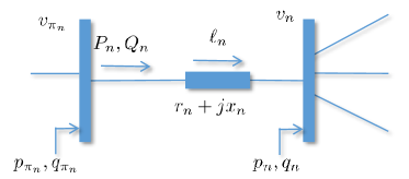
Figure 1: Bus $n$ is connected to its unique parent $\pi_{n}$ via line $n$.

The radial grid can be described by the so-termed branch flow model [2], which enforces the following equations for all $n\in\mathcal{N}$

$$P_{n} =\sum_{j\in\chi_{n}}P_{j}-p_{n}+r_{n}\ell_{n}$$ (1a)

$$Q_{n} =\sum_{j\in\chi_{n}}Q_{j}-q_{n}+x_{n}\ell_{n}$$ (1b)

$$v_{n} ={v_{\pi_{n}}}\!-2(r_{n}P_{n}\!+x_{n}Q_{n})\!+(r_{n}^{2}\!+x_{n}^{2})\ell_{n}$$ (1c)

$$\ell_{n} =\frac{P^{2}_{n}+Q^{2}_{n}}{v_{\pi_{n}}}$$ (1d)

where the set $\chi_{n}\subseteq\mathcal{N}$ collects all children buses for bus $n$.

Traditionally, for a smart inverter located at bus $n$ with nominal power capacity $\bar{s}_{n}$, and a solar panel equipped at this bus with an nameplate active power capacity $\bar{p}^{g}_{n}$, it should hold that $\bar{s}_{n}=\bar{p}^{g}_{n}$. In addition, the reactive power $q^{g}_{n}$ generated by the inverter is constrained by $|q_{n}^{g}|\leq\sqrt{(\bar{s}_{n})^{2}-(p^{g}_{n})^{2}}$, where $p^{g}_{n}$ is the smart inverter output. However, to capture the special scenario that no reactive power can be provided when the maximum inverter output is reached (i.e., $p^{g}_{n}=\bar{p}^{g}_{n}$), oversized inverters’ nameplate capacity (i.e., $\bar{s}_{n}>\bar{p}^{g}_{n}$) is used in practice. For instance, the reactive power compensation provided by inverter $n$ can be $|q_{n}^{g}|\leq 0.4\bar{p}^{g}_{n}$, if choose $\bar{s}_{n}=1.08\bar{p}^{g}_{n}$ and limit $q_{n}^{g}$ to $\sqrt{(\bar{s}_{n})^{2}-(\bar{p}^{g}_{n})^{2}}$ instead of $\sqrt{(\bar{s}_{n})^{2}-(p^{g}_{n})^{2}}$, regardless of the instantaneous PV output $p^{g}_{n}$ [11]. Under this policy, the reactive injection region is the time-invariant convex set

$${\underline{\boldsymbol{q}}^{g}\leq\boldsymbol{q}^{g}\leq\bar{\boldsymbol{q}}^{g}}$$ (2)

where $\boldsymbol{q}^{g}\in\mathcal{R}^{M}$, and $M$ denotes the number of inverters in the grid. Moreover, the voltage magnitude at every bus $n\in\mathcal{N}$ should be maintained within a prespecified range, i.e., $v_{n}\in[\underline{v}_{n},\overline{v}_{n}]$. In practice this range is chosen to be $\pm 5\%$ of its nominal value. For future use, rewrite voltage regulation constraints at all buses $n\in\mathcal{N}$ in a compact way as

$$\boldsymbol{v}\in\mathcal{V}:=\{\boldsymbol{v}:\underline{\boldsymbol{v}}\leq\boldsymbol{v}\leq\overline{\boldsymbol{v}}\}.$$ (3)

In distribution grids, it holds that $p_{n}^{g}=p_{n}^{c}=q_{n}^{c}=0$ and $q_{n}^{g}>0$ when bus $n$ only has a capacitor; while $p_{n}^{g}=q_{n}^{g}=0$, $p^{c}_{n}\geq 0$, $q^{c}_{n}\geq 0$ when bus $n$ is a purely load bus; and a distributed generation bus $n$ not only consumes power denoted by $p_{n}^{c}$, $q_{n}^{c}$, but also generate active power $p_{n}^{g}\geq 0$, and provide negative or positive reactive power $q^{g}_{n}$. Moreover, active power consumption and solar generation $(\boldsymbol{p}^{c},\boldsymbol{q}^{c},\boldsymbol{p}^{g})$ can be predicted through the hourly and real-time market (see e.g., [11]), or by means of running load demand (solar generation) prediction algorithms [20].

III PROBLEM FORMULATION

In the envisioned distribution network operation scenario, active power $\boldsymbol{p}$ is controlled at a coarse timescale. Depending on the variability of active power and cyber resources (sensing, communication, and computation delays), reactive power compensation occurs over time intervals indexed by $t=0,1,\ldots$, which could either be real-time market periods, e.g., $5$ minutes, or even shorter, e.g., $30$ seconds. Let $(\boldsymbol{p}_{t},\boldsymbol{q}_{t})$ denote the active and reactive power injections at all non-root buses during control period $t$. The total power loss across all distribution lines can be expressed as $\sum_{n=1}^{N}r_{n,t}\ell_{n,t}$. Given load consumptions $(\boldsymbol{p}^{c}_{t},\boldsymbol{q}^{c}_{t})$ and generation $\boldsymbol{p}^{g}_{t}$ at the beginning of each interval $t$, the goal of reactive power control is to find feasible reactive power injections ${\boldsymbol{q}}^{g,\ast}_{t}$ for smart inverters such that the power loss across all distribution lines is minimized while maintaining all bus voltage magnitudes within a prescribed range. Formally, the reactive power control problem is formulated as follows

$${\boldsymbol{q}}^{g,\ast}_{t}: =\arg\min_{\underline{\boldsymbol{q}}^{g}\leq\boldsymbol{q}^{g}\leq\bar{\boldsymbol{q}}^{g}}f(\boldsymbol{p}_{t},\boldsymbol{q}^{g}-\boldsymbol{q}^{c}_{t})$$ (4)

where $f(\boldsymbol{p}_{t},\boldsymbol{q}^{g}-\boldsymbol{q}^{c}_{t})$ admits the following form

$$f(\boldsymbol{p}_{t},\boldsymbol{q}^{g}-\boldsymbol{q}^{c}_{t}) =\min_{{\boldsymbol{P}_{t},\boldsymbol{Q}_{t}\atop\bm{\ell}_{t},\boldsymbol{v}_{t}}}\sum_{n=1}^{L}r_{n,t}\ell_{n,t}$$ (5a)

$$\textrm{s.to}~{}~{}P_{n,t} =\sum_{j\in\mathcal{C}_{n,t}}P_{j,t}-p_{n,t}+r_{n,t}\ell_{n,t},~{}n\in\mathcal{N}$$ (5b)

$$Q_{n,t} =\sum_{j\in\mathcal{C}_{n}}Q_{j,t}-q_{n,t}+x_{n,t}\ell_{n,t},\;~{}n\in\mathcal{N}$$ (5c)

$$v_{n,t} =v_{\pi_{n,t}}+(r_{n,t}^{2}+x_{n,t}^{2})\ell_{n,t}$$

$$\quad~{}-2(r_{n,t}P_{n,t}+x_{n,t}Q_{n,t}),~{}~{}\;n\in\mathcal{N}$$ (5d)

$$\ell_{n,t} =\frac{P_{n,t}^{2}+Q_{n,t}^{2}}{v_{\pi_{n,t}}},\qquad\quad\quad~{}~{}~{}~{}~{}n\in\mathcal{E}$$ (5e)

$$\boldsymbol{v} \in\mathcal{V}.$$ (5f)

Clearly, constraints (5b)–(5d) and (5f) are linear with respect to system variables $(\boldsymbol{p}_{t},\boldsymbol{q}_{t},\boldsymbol{P_{t}},\boldsymbol{Q_{t}},\bm{\ell_{t}},\boldsymbol{v_{t}})$. Nevertheless, constraints in (5e) are quadratic equalities, depicting a non-convex feasible set and rendering the optimization problem non-convex and NP-hard in general [7].

To address this issue, these equalities in (5e) have been recently relaxed to convex inequalities described by the hyperbolic constraints [7]

$$P^{2}_{n,t}+Q^{2}_{n,t}\leq{v_{\pi_{n,t}}}\ell_{n,t}.$$ (6)

Substituting (6) into (5) yields

$$f(\boldsymbol{p}_{t},\boldsymbol{q}_{t})~{} =\min_{{\boldsymbol{P}_{t},\boldsymbol{Q}_{t}\atop\bm{\ell}_{t},\boldsymbol{v}_{t}}}\sum_{n=1}^{L}r_{n,t}\ell_{n,t}$$ (7a)

s.to $$\eqref{eq:spf}-\eqref{eq:svf},{\rm~{}and~{}}\eqref{eq:sVf}$$ (7b)

$$\ell_{n,t} \geq\frac{P_{n,t}^{2}+Q_{n,t}^{2}}{v_{\pi_{n,t}}},~{}n\in\mathcal{E}$$ (7c)

where (7c) can also be equivalently expressed as a second-order cone

$$\!\left\|\begin{array}[]{c}2P_{n,t}\\ 2Q_{n,t}\\ \ell_{n,t}-v_{\pi_{n,t}}\end{array}\right\|\leq v_{\pi_{n,t}}+\ell_{n,t}.$$ (11)

Constraints (7b) and (7c) represent now a convex feasible set, and the problem in (7) can be solved by standard convex programming methods. Interestingly, it has been shown that under certain conditions, at the optimal solution of (7), equalities are attained in (11); see details in e.g., [gan2012exactnessconvex]. In this case, the optimal solution of the original problem (5) is recovered too.

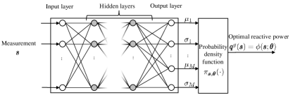
Figure 2: Statistical learning architecture.

It is worth pointing out that problem (4) formally characterizes the optimal reactive power control policies for a diverse set of networked control problems, including e.g., voltage regulation, Volt/VAR control, and optimal power flow [gan2012exactnessconvex], by choosing suitable objective functions. If active and reactive power injections $(\boldsymbol{p}_{t},\boldsymbol{q}_{t}^{c})$ were both known precisely in advance and remained constant within period $t$, the optimal reactive power compensation $\boldsymbol{q}^{g,\ast}_{t}$ would be found by solving (4). However, such conditions are hardly met in contemporary distribution systems, due partly to i) time-varying active and reactive injections; and, ii) noise-contaminated observations caused by direct measurements, delayed estimates, or inaccurate forecasts. To bypass these challenges, minimizing the averaged power loss over the power injections $(\boldsymbol{p}_{t},\boldsymbol{q}_{t}^{c})$ provides an alternative to the static reactive power control formulation in (4), given by

$$\boldsymbol{q}^{g,\ast}_{t}:=\arg\min_{\underline{\boldsymbol{q}}^{g}\leq\boldsymbol{q}^{g}\leq\bar{\boldsymbol{q}}^{g}}~{}\mathbb{E}\left[f(\boldsymbol{p}_{t},\boldsymbol{q}^{g}-\boldsymbol{q}^{c}_{t})\right].$$ (12)

For notational convenience, let us define the state vector $\boldsymbol{s}_{t}:=(\boldsymbol{p}_{t},\boldsymbol{q}^{c}_{t})$, which is assumed to be a stationary random process, and rewrite the loss function $f(\boldsymbol{p}_{t},\boldsymbol{q}^{g}-\boldsymbol{q}^{c}_{t})$ as $f(\boldsymbol{q}^{g};\boldsymbol{s}_{t})$. Substituting this display into the original problem (12), yields

$$\boldsymbol{q}^{g,\ast}(\boldsymbol{s}_{t}):=\arg\min_{\underline{\boldsymbol{q}}^{g}\leq\boldsymbol{q}^{g}\leq\bar{\boldsymbol{q}}^{g}}~{}\mathbb{E}\left[f(\boldsymbol{q}^{g};\boldsymbol{s}_{t})\right].$$ (13)

Rather than the unreliable and possibly obsolete instantaneous $\boldsymbol{q}^{g,\ast}_{t}$ found through (4), problem (13) is expected to yield smoother power control decisions. But, evaluating the expectation in (13) is nearly impossible in practice, even if the probability density function of $\boldsymbol{s}_{t}$ was known. Challenge also comes from the computational burden of dealing with the non-convex constraint (5e). To approximate $\boldsymbol{q}^{g,\ast}$ in a computationally efficient manner, a statistical learning approach is developed next.

IV STATISTICAL LEARNING

The rapid growth in renewable generation is displacing traditional forms of energy generation while increasing the need for controllable and flexible resources to balance fluctuations in load and generation. In this section, we introduce a novel parameterization form of the reactive power control problem, as well as a learning solver based on a deep neural network.

IV-A Parameterization

Instead of solving (13) exactly, consider a parametrization for the reactive power compensation as follows

$$\boldsymbol{q}^{g}=\phi(\boldsymbol{s};\boldsymbol{\theta})$$ (14)

where $\phi(\boldsymbol{s};\boldsymbol{\theta})$ is some function given by e.g., a deep neural network, and $\boldsymbol{\theta}\in\mathbb{R}^{d}$ collects all unknown parameters. Building on this, finding the optimal reactive power control $\boldsymbol{q}^{g,\ast}$ in (13) boils down to finding the optimal parameter vector $\boldsymbol{\theta}^{\ast}$, such that the expected loss is minimized; that is,

$$\boldsymbol{\theta}^{\ast}=\arg\min_{\boldsymbol{\theta}}~{} \mathbb{E}\left[f(\phi(\boldsymbol{s};\boldsymbol{\theta});\boldsymbol{s})\right].$$ (15)

To find $\boldsymbol{\theta}^{\ast}$, a natural approach is to apply gradient descent type algorithms. To this aim, one needs to obtain the gradient of the objective function in (15) with respect to $\boldsymbol{\theta}$, i.e., $\nabla_{\boldsymbol{\theta}}\mathbb{E}\left[f(\phi(\boldsymbol{s};\boldsymbol{\theta});\boldsymbol{s})\right]$. In practice however, there is no analytic form of $f(\phi(\boldsymbol{s};\boldsymbol{\theta});\boldsymbol{s})$ as a function of $\phi(\boldsymbol{s};\boldsymbol{\theta})$ or $\boldsymbol{\theta}$. In (5), for instance, the loss function $f$ depends only implicitly on $\boldsymbol{q}^{g}$. Instead, we can observe the function value $f$ for any grid operating point $(\boldsymbol{p},\boldsymbol{q},\boldsymbol{P},\boldsymbol{Q},\bm{\ell},\boldsymbol{v})$ [cf. (5)], which can be used to estimate the gradient. This motivates development of a model-free approach [5]. Specifically, for a given set of iterates and reactive power realizations $\{\tilde{\boldsymbol{\theta}},\tilde{\boldsymbol{q}^{g}}\}$, the corresponding loss function values $\tilde{f}(\tilde{\boldsymbol{q}}^{g}_{\boldsymbol{\theta}};\boldsymbol{s})$ can be observed from the system. Using $\{\tilde{\boldsymbol{\theta}},\tilde{\boldsymbol{q}^{g}}\}$ and $\tilde{f}(\tilde{\boldsymbol{q}}^{g}_{\boldsymbol{\theta}};\boldsymbol{s})$, the parameter vector $\boldsymbol{\theta}$ can be updated through the policy gradient method [15], which constructs a gradient estimate with only function observations.

A control policy here is a mapping from state vectors $\boldsymbol{s}$ to reactive power control decisions (a.k.a. actions) $\boldsymbol{q}^{g}$. Consider first the stochastic control policy $\pi:\boldsymbol{s}\rightarrow\boldsymbol{q}^{g}$, specifying a conditional distribution of all possible decisions $\boldsymbol{q}^{g}$ given the current state $\boldsymbol{s}$. Denoting the probability of taking action $\boldsymbol{q}^{g}$ at state $\boldsymbol{s}$ as $\pi_{\boldsymbol{s},\boldsymbol{\theta}}(\boldsymbol{q}^{g})$, the gradient of $\mathbb{E}\left[f(\phi(\boldsymbol{s};\boldsymbol{\theta});\boldsymbol{s})\right]$ with respect to $\boldsymbol{\theta}$ can be written as

$$\nabla_{\boldsymbol{\theta}}\mathbb{E}\left[f(\phi(\boldsymbol{s};\boldsymbol{\theta});\boldsymbol{s})\right]=\nabla_{\boldsymbol{\theta}}\int_{\boldsymbol{s}}f(\phi(\boldsymbol{s};\boldsymbol{\theta});\boldsymbol{s})\textrm{Pr}(\boldsymbol{s})d{\boldsymbol{s}}$$ (16a)

$$=\nabla_{\boldsymbol{\theta}}\int_{\boldsymbol{s}}\int_{\boldsymbol{q}^{g}}f(\boldsymbol{q}^{g};\boldsymbol{s})\pi_{\boldsymbol{s},\boldsymbol{\theta}}(\boldsymbol{q}^{g})\textrm{Pr}(\boldsymbol{s})d{\boldsymbol{q}^{g}}d{\boldsymbol{s}}$$ (16b)

$$=\int_{\boldsymbol{s}}\int_{\boldsymbol{q}^{g}}f(\boldsymbol{q}^{g};\boldsymbol{s})\frac{\nabla_{\boldsymbol{\theta}}\pi_{\boldsymbol{s},\boldsymbol{\theta}}(\boldsymbol{q}^{g})}{\pi_{\boldsymbol{s},\boldsymbol{\theta}}(\boldsymbol{q}^{g})}\pi_{\boldsymbol{s},\boldsymbol{\theta}}(\boldsymbol{q}^{g})\textrm{Pr}(\boldsymbol{s})d{\boldsymbol{q}^{g}}d{\boldsymbol{s}}$$ (16c)

$$=\mathbb{E}_{\boldsymbol{q}^{g},\boldsymbol{s}}\left[f(\boldsymbol{q}^{g};\boldsymbol{s})\nabla_{\boldsymbol{\theta}}\textrm{log}\pi_{\boldsymbol{s},\boldsymbol{\theta}}(\boldsymbol{q}^{g})\right]$$ (16d)

where $\textrm{Pr}(\boldsymbol{s})$ denotes the probability of state $\boldsymbol{s}$, and $\boldsymbol{q}^{g}$ is drawn from the distribution $\pi_{\boldsymbol{s},\boldsymbol{\theta}}(\cdot)$. Here, the computation of $\nabla_{\boldsymbol{\theta}}\mathbb{E}\left[f(\phi(\boldsymbol{s};\boldsymbol{\theta});\boldsymbol{s})\right]$ is translated to evaluating the expectation of function $f(\boldsymbol{q}^{g};\boldsymbol{s})$ multiplied by the gradient of the policy distribution $\nabla_{\boldsymbol{\theta}}\textrm{log}\pi_{\boldsymbol{s},\boldsymbol{\theta}}(\boldsymbol{q}^{g})$. This is indeed useful when we have an analytic form for $\pi_{\boldsymbol{s},\boldsymbol{\theta}}(\boldsymbol{q}^{g})$. In such case, we may further replace the expectation on the right-hand side (16) with a sample mean. Specifically, by using previous function observations, we obtain the following gradient estimate

$$\widehat{\nabla_{\boldsymbol{\theta}}\mathbb{E}}\left[f(\phi(\boldsymbol{s};\boldsymbol{\theta});\boldsymbol{s})\right]=\hat{f}(\hat{\boldsymbol{q}}^{g}_{\boldsymbol{\theta}};\boldsymbol{s})\nabla_{\boldsymbol{\theta}}\textrm{log}\pi_{\boldsymbol{s},\boldsymbol{\theta}}(\hat{\boldsymbol{q}}^{g}_{\boldsymbol{\theta}})$$ (17)

where $\hat{\boldsymbol{q}}^{g}_{\boldsymbol{\theta}}$ is the injected reactive power into the distribution grid, drawn from the distribution $\pi_{\boldsymbol{s},\boldsymbol{\theta}}(\cdot)$, and $\hat{f}(\hat{\boldsymbol{q}}^{g}_{\boldsymbol{\theta}};\boldsymbol{s})$ is the corresponding observed loss function value obtained by solving (5).

Previously, it was assumed that the policy $\phi(\boldsymbol{s};\boldsymbol{\theta})$ is stochastic. In deterministic cases, where the distribution is a delta function, i.e., $\pi_{\boldsymbol{s},\boldsymbol{\theta}}(\boldsymbol{x})=\delta(\boldsymbol{x}-\phi(\boldsymbol{s};\boldsymbol{\theta}))$. To evaluate $\nabla_{\boldsymbol{\theta}}\textrm{log}\pi_{\boldsymbol{s},\boldsymbol{\theta}}(\hat{\boldsymbol{q}}^{g}_{\boldsymbol{\theta}})$ in (17), one may approximate the delta function with a known density function centered around $\phi(\boldsymbol{s};\boldsymbol{\theta})$. To capture the power constraint ${\underline{\boldsymbol{q}}^{g}\leq\boldsymbol{q}^{g}_{t}\leq\bar{\boldsymbol{q}}^{g}}$, a truncated Gaussian distribution with a fixed support on the domain $[\underline{\boldsymbol{q}}^{g},\bar{\boldsymbol{q}}^{g}]$ is considered in next subsection.

IV-B Model-free learning

To find the policy $\pi_{\boldsymbol{s},\boldsymbol{\theta}}(\cdot)$, we restrict ourselves to the increasingly popular set of parameterizations, known as deep neural networks [8]. Indeed, deep neural networks have recently demonstrated remarkable performance in numerous fields, including computer vision, speech recognition, and robotics. A deep neural network can effectively tackle the ‘curse of dimensionality’ by extracting low-dimensional representation for high-dimensional data [8].

Consider a feed-forward deep neural network connected to a truncated Gaussian probability density function $\pi_{\boldsymbol{s},\boldsymbol{\theta}}(\cdot)$ block; see Fig. 2 for an illustration. It takes as input the state vector $\boldsymbol{s}$, followed by $L$ fully connected hidden layers with ReLU activation functions. The output of the deep neural network is a set of mean and standard deviation pairs $\{\mu_{m},\sigma_{m}\}_{m=1}^{M}$, each corresponding to $M$ truncated Gaussian distributions. By feeding the outputs of the deep neural network into the probability density function $\pi_{\boldsymbol{s},\boldsymbol{\theta}}(\cdot)$ block, the reactive power compensation vector $\boldsymbol{q}^{g}$ is sampled from $\pi_{\boldsymbol{s},\boldsymbol{\theta}}(\boldsymbol{q}^{g})$. Stacking all the weights of the deep neural network into the vector $\boldsymbol{\theta}$, we have a function approximation to estimate the reactive power compensation $\boldsymbol{q}^{g}(\boldsymbol{s})=\phi(\boldsymbol{s};\boldsymbol{\theta})$.

Using the gradient estimate in (17), the weights $\boldsymbol{\theta}$ can be successively updated as follows

$$\boldsymbol{\theta}_{t+1}=\boldsymbol{\theta}_{t}-\beta_{t}\widehat{\nabla_{\boldsymbol{\theta}}\mathbb{E}}\left[f({\phi}(\boldsymbol{s}_{t};\boldsymbol{\theta});\boldsymbol{s}_{t})\right]\Big{|}_{\boldsymbol{\theta}=\boldsymbol{\theta}_{t}}$$ (18)

where $\beta_{t}>0$ is a preselected learning rate. This update in (18) is a model-free approach, since it does not require explicit knowledge about the actual form of the function $f(\cdot)$ or distribution of $\boldsymbol{s}$. Different from a traditional supervised approach where requires a set of a given training labeled data [20], the developed method here is unsupervised; hence circumvents the need for labeled data and directly solves (13).

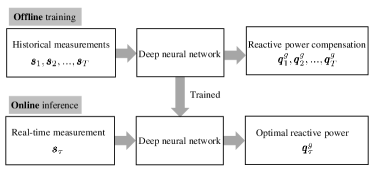
Figure 3: Two phases reactive power control procedure

Algorithm 1 A statistical learning approach to reactive power control

Training phase:

1:Initialize: $\boldsymbol{\theta}$.

2:for $t=1,2,\ldots,T$  do

3:     Observe historical measurement $\boldsymbol{s}_{t}$.

4:     Feed $\boldsymbol{s}_{t}$ into the deep neural network.

5:     Obtain deep neural network output mean $\boldsymbol{\mu}_{t}$ and variance $\boldsymbol{\sigma}_{t}$.

6:     Feed $\boldsymbol{\mu}_{t}$ and $\boldsymbol{\sigma}_{t}$ into $\pi_{\boldsymbol{s}_{t},\boldsymbol{\theta}_{t}}(\cdot)$.

7:     Draw a sample $\hat{\boldsymbol{q}}^{g}_{\boldsymbol{\theta}_{t}}$ from the distribution $\pi_{\boldsymbol{s}_{t},\boldsymbol{\theta}_{t}}(\boldsymbol{q}^{g})$.

8:     Obtain an estimate for $\hat{f}(\boldsymbol{s}_{t},\hat{\boldsymbol{q}}^{g}_{\boldsymbol{\theta}_{t}})$ via (7).

9:     Calculate $\widehat{\nabla_{\boldsymbol{\theta}}\mathbb{E}}\left[f(\boldsymbol{s}_{t},\phi(\boldsymbol{s}_{t};\boldsymbol{\theta}_{t}))\right]$ via (17).

10:     Update $\boldsymbol{\theta}_{t+1}$ according to (18).

11:end for

Inference phase:

1:for $\tau=1,2,\ldots$ do

2:     Feed real-time measurement $\boldsymbol{s}_{\tau}$ into the trained deep neural network.

3:     Obtain the deep neural network output mean $\boldsymbol{\mu}_{\tau}$ and variance $\boldsymbol{\sigma}_{\tau}$.

4:     Feed $\boldsymbol{\mu}_{\tau}$ and $\boldsymbol{\sigma}_{\tau}$ into $\pi_{\boldsymbol{s}_{\tau},\boldsymbol{\theta}_{\tau}}(\cdot)$.

5:     Draw a sample $\hat{\boldsymbol{q}}^{g}_{\boldsymbol{\theta}_{\tau}}$ from the distribution $\pi_{\boldsymbol{s}_{\tau},\boldsymbol{\theta}_{\tau}}(\boldsymbol{q}^{g})$.

6:end for

The proposed reactive power control procedure is tabulated in Alg. 1. It is implemented in two phases, namely offline training and online inference phases, as shown in Fig 3. Specifically, in the training phase, historical/simulated datum $\boldsymbol{s}$ is fed into the deep neural network. For a given input datum $\boldsymbol{s}_{t}$, our network spits out a reactive power compensation $\boldsymbol{q}^{g}_{t}=\phi(\boldsymbol{s}_{t};\boldsymbol{\theta}_{t})$. Subsequently, the distribution network returns a loss for this state-action pair $(\boldsymbol{s}_{t},\boldsymbol{q}^{g}_{t})$ (which can also be found by solving (5)). Finally, a gradient estimate can be obtained using the policy gradient method in (17), based on which the neural network weight parameters are updated following (18). The trained deep neural network will be utilized in the inference phase. By taking the real-time state vector $\boldsymbol{s}_{t}=(\boldsymbol{p}_{t},\boldsymbol{q}^{c}_{t})$ as input, the trained deep neural network outputs the optimal reactive power compensation $\boldsymbol{q}^{g}_{t}$ to be implemented in the grid. Note that the proposed statistical learning approach is desirable for real-time reactive power control, as it shifts the computational burden of tackling non-convex optimization to offline training of a neural network.

V NUMERICAL TESTS

In this section, the performance of our proposed statistical learning scheme was evaluated on a real-world $47$-bus feeder with high penetration of renewables [6]; see Fig. 4. This feeder is integrated with $M=5$ smart inverters located on buses $2$, $16$, $18$, $21$, and $22$, with capacities $300$, $80$, $300$, $400$, and $200$ kW, respectively. A power factor of $0.8$ was assumed for all loads.

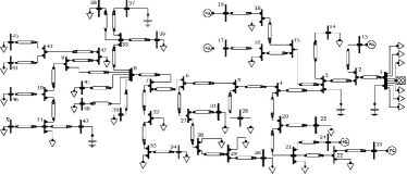
Figure 4: Schematic diagram of the $47$-bus distribution feeder.

The training and test data were obtained by splitting the consumption and solar generation from the Smart^∗ project collected on August 24, 2011 [3]. The CVX toolbox [9] was used to solve the SOCP problem in (7) to evaluate $\hat{f}(\hat{\boldsymbol{q}}^{g}_{\boldsymbol{\theta}};\boldsymbol{s})$. The deep neural network used here consists of three fully connected hidden layers, with $48$, $32$ and $16$ neurons per layer, respectively. To carry out the simulations, we used ‘TensorFlow’ [1] on an NVIDIA Titan X GPU with 12 GB RAM. The weight parameters of the deep neural network were updated using the back-propagation algorithm with ‘Adam’ optimizer. The learning rate was fixed to $0.001$, and the batch size was $30$ throughout $40$ epochs of tests.

To assess the performance of the proposed approach, the following baseline was considered. Assuming perfect observations of active and reactive power injections $(\boldsymbol{p}_{t},\boldsymbol{q}_{t}^{c})$ at the beginning of slot $t$, the optimal reactive power control can be found by solving the following problem

$$f(\boldsymbol{p}_{t},\boldsymbol{q}^{g}_{t}-\boldsymbol{q}^{c}_{t})=\min_{\boldsymbol{q}^{g}_{t},\boldsymbol{P}_{t},\boldsymbol{Q}_{t}\atop\bm{\ell}_{t},\boldsymbol{v}_{t}}~{} \sum_{n=1}^{L}r_{n,t}\ell_{n,t}$$ (19a)

s.to $$\eqref{eq:relax1}-\eqref{eq:relax2}$$ (19b)

where $\boldsymbol{q}^{g}_{t}$ is treated as an optimization variable. It should be noted that tackling this problem in real-time is computationally expensive, while the proposed approach finds $\boldsymbol{q}^{g}_{t}$ after performing only several matrix-vector multiplications. The red curve in Fig. 5 shows the observed loss for the proposed approach, while the blue one depicts loss for the deterministic optimal one obtained via (19) during the training phase. The light colour curves correspond to the actual observed losses, while the dark ones are the running averaged ones. Clearly, our model-free approach learns to make optimal decisions $\boldsymbol{q}^{g}_{t}$. In the inference phase, the loss of the proposed approach versus the baseline is presented in Fig. 6. This plot demonstrates that the proposed model-free approach finds near-optimal reactive power control decisions. The running time of the proposed approach is one order of magnitude less than the optimization-based approach.

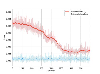
Figure 5: The training loss of the statistical learning approach compared with the baseline (optimal).

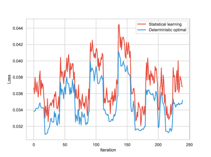
Figure 6: The inference loss values of statistical learning approach and the baseline (optimal).

VI CONCLUSIONS

In this work, a statistical learning framework for reactive power control in distribution grids was developed. Uncertainties and delays in acquiring grid state motivate well this learning framework. The non-convexity of the underlying optimization, and lack of model knowledge makes reactive power control a challenge in modern grids, if not impossible, to solve directly. The theory of statistical learning empowered by non-linear functional approximation property of deep neural networks provided a fresh viewpoint to solve this problem. In particular, this work modeled the reactive power control policy via a deep neural network. The weights of the deep neural network were updated in an unsupervised and model-free fashion, circumventing the need for labeled data as well as an explicit model for the system. Our proposed method is computationally inexpensive, since all computational complexity is shifted to the training phase. Preliminary numerical results on the real-world $47$-bus distribution network using real load data corroborate the merits of our developed approach. This work opens up several interesting directions for future research. Robust methods for reactive power control in the presence of corrupted or adversarial observations is worth investigating. Exploiting topology of the power grid to design physics-informed architecture is also pertinent.

References

- [1] M. Abadi, A. Agarwal, P. Barham, E. Brevdo, Z. Chen, C. Citro, G. S. Corrado, A. Davis, J. Dean, M. Devin et al., “Tensorflow: Large-scale machine learning on heterogeneous distributed systems,” arXiv:1603.04467, 2016.
- [2] M. Baran and F. F. Wu, “Optimal sizing of capacitors placed on a radial distribution system,” IEEE Trans. Power Del., vol. 4, no. 1, pp. 735–743, Jan. 1989.
- [3] S. Barker, A. Mishra, D. Irwin, E. Cecchet, P. Shenoy, and J. Albrecht, “Smart*: An open data set and tools for enabling research in sustainable homes,” SustKDD, vol. 111, no. 112, p. 108, Aug. 2012.
- [4] P. M. Carvalho, P. F. Correia, and L. A. Ferreira, “Distributed reactive power generation control for voltage rise mitigation in distribution networks,” IEEE Trans. Power Syst., vol. 23, no. 2, pp. 766–772, April 2008.
- [5] M. Eisen, C. Zhang, L. F. Chamon, D. D. Lee, and A. Ribeiro, “Learning optimal resource allocations in wireless systems,” IEEE Trans. Signal Process., vol. 67, no. 10, pp. 2775–2790, 2019.
- [6] M. Farivar, C. R. Clarke, S. H. Low, and K. M. Chandy, “Inverter VAR control for distribution systems with renewables,” in Proc. of SmartGridComm., Brussels, Belgium, Oct. 2011, pp. 457–462.
- [7] L. Gan, N. Li, U. Topcu, and S. Low, “On the exactness of convex relaxation for optimal power flow in tree networks,” in Proc. of Conf. Decision and Control, Maui, HI, USA, Dec. 2012, pp. 465–471.
- [8] I. Goodfellow, Y. Bengio, and A. Courville, Deep Learning. Cambridge, MA: MIT press, 2016.
- [9] M. Grant and S. Boyd, “CVX: Matlab software for disciplined convex programming, version 2.1,” 2014.
- [10] M. Jalali, V. Kekatos, N. Gatsis, and D. Deka, “Designing reactive power control rules for smart inverters using support vector machines,” arXiv:1903.01016, 2019.
- [11] V. Kekatos, G. Wang, A. J. Conejo, and G. B. Giannakis, “Stochastic reactive power management in microgrids with renewables,” IEEE Trans. Power Syst., vol. 30, no. 6, pp. 3386–3395, Dec. 2015.
- [12] W. Lee, M. Kim, and D. Cho, “Deep power control: Transmit power control scheme based on convolutional neural network,” IEEE Commun. Lett., vol. 22, no. 6, pp. 1276–1279, June 2018.
- [13] W. Lin, R. Thomas, and E. Bitar, “Real-time voltage regulation in distribution systems via decentralized PV inverter control,” in Proc. of Hawaii Intl. Conf. System Sciences, Waikoloa Village, Hawaii, Jan. 2-6, 2018.
- [14] O. Sondermeijer, R. Dobbe, D. Arnold, C. Tomlin, and T. Keviczky, “Regression-based inverter control for decentralized optimal power flow and voltage regulation,” arXiv:1902.08594, 2019.
- [15] R. S. Sutton, D. A. McAllester, S. P. Singh, and Y. Mansour, “Policy gradient methods for reinforcement learning with function approximation,” in Proc. of Adv. Neural Inf. Process. Syst., 2000, pp. 1057–1063.
- [16] G. Wang, V. Kekatos, A. J. Conejo, and G. B. Giannakis, “Ergodic energy management leveraging resource variability in distribution grids,” IEEE Trans. Power Syst., vol. 31, no. 6, pp. 4765–4775, Nov. 2016.
- [17] Q. Yang, G. Wang, A. Sadeghi, G. B. Giannakis, and J. Sun, “Two-timescale voltage control in distribution grids using deep reinforcement learning,” arXiv:1904.09374, 2019.
- [18] A. Zamzam and K. Baker, “Learning optimal solutions for extremely fast AC optimal power flow,” arXiv:1910.01213, 2019.
- [19] A. S. Zamzam and N. D. Sidiropoulos, “Physics-aware neural networks for distribution system state estimation,” arXiv:1903.09669, 2019.
- [20] L. Zhang, G. Wang, and G. B. Giannakis, “Real-time power system state estimation and forecasting via deep unrolled neural networks,” IEEE Trans. Signal Process., vol. 67, no. 15, pp. 4069–4077, Aug. 2019.
- [21] Y. Zhang, M. Hong, E. Dall’Anese, S. V. Dhople, and Z. Xu, “Distributed controllers seeking AC optimal power flow solutions using ADMM,” IEEE Trans. Smart Grid, vol. 9, no. 5, pp. 4525–4537, Sept. 2018.
- [22] Y. Zhao, J. Chen, and H. V. Poor, “A learning-to-infer method for real-time power grid multi-line outage identification,” IEEE Trans. Smart Grid, pp. 1–1, 2019.
- [23] H. Zhu and H. J. Liu, “Fast local voltage control under limited reactive power: Optimality and stability analysis,” IEEE Trans. Power Syst., vol. 31, no. 5, pp. 3794–3803, Dec. 2016.