OUTP-19-12P, CERN-TH-2019-180, TTP19-035, P3H-19-040

Analytic results for deep-inelastic scattering at NNLO QCD with the nested soft-collinear subtraction scheme

We present analytic results that describe fully-differential NNLO QCD corrections to deep-inelastic scattering processes within the nested soft-collinear subtraction scheme. This is the last building block required for the application of this scheme to computations of NNLO QCD corrections to arbitrary processes at hadron colliders.

1 Introduction

In this paper, we apply the nested soft-collinear subtraction scheme for NNLO QCD computations, introduced by some of us in Ref. [1], to the deep-inelastic scattering (DIS) process $Pe\to e+X$. We note right away that our goal is not DIS phenomenology; rather, we would like to extend this subtraction scheme to processes that involve QCD partons in both the initial and the final state.

Compared to the cases of color singlet production [2] and decay [3] that we studied earlier, the DIS process requires us to deal with the situation where QCD partons in the (leading order) hard processes are not back-to-back. This makes the computation of NNLO QCD corrections to deep-inelastic scattering an important next step in the development of the nested subtraction scheme (NSS).

In spite of the fact that the computation that we report in this paper is new, we would like to emphasize that we can re-use significant parts of the analytic computations described in Refs. [2, 3]. This is so because collinear singularities in QCD factorize on external lines so that their treatment, including analytic integration of respective subtraction terms [4], is process-independent. Hence, everything that needs to be known about collinear singularities in DIS and their regularization can be inferred from the treatment of the collinear singularities in color-singlet production and color-singlet decays, see Refs. [2, 3].

At variance with collinear limits, important differences arise in the treatment of the (double-) soft radiation which is sensitive to the relative orientation of three-momenta of hard emittors. The integrated double-soft subtraction term for the case when the momenta of hard emittors are at an angle to each other was analytically computed in Ref. [5]. The computation of NNLO QCD corrections to the DIS process that we report in this paper is the first application of that result.

The main result of this paper is the set of analytic formulas that, in conjunction with the fully-resolved regulated contribution, provides a fully-differential description of DIS at NNLO QCD. It is our long-term goal to employ these formulas as ingredients to describe “initial-final dipole” contributions when computing NNLO QCD corrections to generic processes. Because of that, it is important to ensure that the analytic results for initial-final dipoles reported in this paper are correct. Studies of DIS are advantageous from this perspective since analytic results for DIS coefficient functions at NNLO are available [6, 7, 8] and we can use them to check our computations to a very high precision.

We note in passing that, in the past decade, a large number of subtraction schemes and slicing methods appeared [9, 10, 11, 12, 13, 14, 15, 16, 17, 18, 19, 20, 21, 22, 23, 24]; they enabled a large number of NNLO QCD computations for important LHC processes [25, 26, 27, 28, 29, 30, 31, 32, 33, 34, 35, 36, 37, 38, 39]. Nevertheless, in spite of all successes, the construction of a fully local, analytic, physically transparent and scalable subtraction scheme remains an interesting challenge. We believe that further development of the NSS, that we describe in this paper, will contribute to finding an answer to this challenge.

The remainder of the paper is organized as follows. In Section 2 we describe how leading order (LO) and next-to-leading order (NLO) DIS cross sections are computed. In Section 3 we discuss the NNLO computation. In Section 4 we validate our results against analytic ones. We conclude in Section 5. Useful formulas are collected in several Appendices. Analytic results for NNLO QCD DIS subtraction terms in computer-readable format are provided in an ancillary file attached to this submission.

2 LO and NLO calculation

We consider deep-inelastic scattering of an electron on a proton

$$P(P_{1})+e(p_{2})\to e(p_{3})+X,$$ (2.1)

mediated by a neutral current. The cross section of this process is computed as a convolution of parton distribution functions with the partonic cross section that describes parton-electron scattering. Schematically, we write

$${\rm d}\sigma_{H}=\sum\limits_{i}\;\int\limits_{0}^{1}{\rm d}x\;f_{i}(x)\;{\rm d}\hat{\sigma}_{f_{i}+e\to X}(xP_{1},p_{2}).$$ (2.2)

In Eq. (2.2) we denote a parton of type $i\in[-5,...,5]$ as $f_{i}$, with $f_{0}=g$ and $f_{\pm 1,\pm 2,\pm 3,\pm 4,\pm 5}=\{d/\bar{d},u/\bar{u},s/\bar{s},c/\bar{c},b/\bar{b}\}$. With a slight abuse of notation, we also use $f_{i}(x)$ to denote the parton distribution function of parton $f_{i}$.

The partonic cross section ${\rm d}\hat{\sigma}_{f_{i}+e\to X}$ can be computed in QCD perturbation theory as an expansion in the strong coupling constant $\alpha_{s}$. We write

$${\rm d}\hat{\sigma}_{f_{i}+e\to X}={{\rm d}\hat{\sigma}}_{f_{i}}^{\rm LO}+{{\rm d}\hat{\sigma}}_{f_{i}}^{\rm NLO}+{{\rm d}\hat{\sigma}}_{f_{i}}^{\rm NNLO}+{\cal O}(\alpha_{s}^{3}).$$ (2.3)

At leading order, electron-quark and electron-anti-quark scattering processes

$$\begin{split}q(p_{1})+e^{-}(p_{2})&\to e^{-}(p_{3})+q(p_{4})\,,\\ \bar{q}(p_{1})+e^{-}(p_{2})&\to e^{-}(p_{3})+\bar{q}(p_{4})\,,\end{split}$$ (2.4)

contribute. For the purpose of computing QCD corrections, there is no difference between these two processes and we focus on the electron-quark scattering.

To compute the partonic cross section of this process, we employ the notation that has been used in earlier papers on the NSS [1, 2, 3], and define

$$\begin{split}\left\langle F_{\rm LM}(1_{q},2_{e},3_{e},4_{q}){\cal O}(\{1,2,3,4\})\right\rangle&\equiv~{}{\cal N}\int[df_{3}][df_{4}]\;(2\pi)^{d}\delta^{(d)}(p_{3}+p_{4}-p_{1}-p_{2})\;\\ &\quad\times|\mathcal{A}^{\rm tree}|^{2}(1_{q},2_{e},3_{e},4_{q})\mathcal{O}(\{p_{1},p_{2},p_{3},p_{4}\})\,,\end{split}$$ (2.5)

where ${\cal N}$ includes normalization and symmetry factors, $d=4-2\epsilon$ is the space-time dimensionality,

$$[df_{i}]=\frac{{\rm d}^{d-1}p_{i}}{(2\pi)^{d-1}2E_{i}}\;\theta(E_{\rm max}-E_{i})\,,$$ (2.6)

is the phase-space volume of a parton $f_{i}$, $\mathcal{A}^{\rm tree}$ is the tree-level matrix element and ${\cal O}$ is a generic observable that depends on momenta $p_{1,..,4}$. $E_{\rm max}$ is a sufficiently large but otherwise arbitrary parameter that provides an upper bound on energies of individual partons; its role will become clear later. We will also use the notation $\left\langle F_{\rm LM}(i,j,...)\right\rangle_{\delta}$ to indicate that the corresponding cross section is fully-differential with respect to momenta that are shown as arguments of the function $F_{\rm LM}$. In this notation, the fully differential LO cross section for quark-electron scattering reads

$$2s\cdot{{\rm d}\hat{\sigma}}_{q}^{{\rm LO}}=\left\langle F_{\rm LM}(1_{q},2_{e},3_{e},4_{q})\right\rangle_{\delta},$$ (2.7)

where $s=2p_{1}\cdot p_{2}$ is the partonic center-of-mass energy squared.

We now discuss NLO QCD corrections. As we already emphasized in Refs. [1, 2, 3], at this order in the $\alpha_{s}$ expansion, our subtraction scheme is equivalent to the FKS one [40, 41]. In spite of that, it is useful to discuss the NLO QCD computation of DIS here, if only to develop a familiarity with our notation. At NLO QCD, both the quark $q/\bar{q}+e\to q/\bar{q}+e+g$ and the gluon $g+e\to q+\bar{q}+e$ channels contribute to the DIS cross section. We consider the quark channel first, and start by discussing the real emission contribution. For the sake of definiteness, we focus on the following process

$$q(p_{1})+e^{-}(p_{2})\to e^{-}(p_{3})+q(p_{4})+g(p_{5})\,.$$ (2.8)

In analogy with Eq. (2.5), we define

$$\begin{split}&\left\langle F_{\rm LM}(1_{q},2_{e},3_{e},4_{q},5_{g}){\cal O}(\{1,2,3,4,5\})\right\rangle\equiv{\cal N}\int\prod_{i=3}^{5}[df_{i}]\;(2\pi)^{d}\delta^{(d)}\left(p_{1}+p_{2}-\sum_{i=3}^{5}p_{i}\right)\\ &\quad\times|\mathcal{A}^{\rm tree}|^{2}(1_{q},2_{e},3_{e},4_{q},5_{g})\mathcal{O}(\{p_{1},p_{2},p_{3},p_{4},p_{5}\}).\end{split}$$ (2.9)

The scattering amplitude is singular when the gluon $g_{5}$ is soft or when it is collinear to the incoming or outgoing quark. Following our earlier work on the NSS [1, 2, 3], we introduce operators $S_{5}$ and $C_{51},C_{54}$ to extract the leading soft and collinear behavior of scattering amplitudes squared, and use these operators to isolate non-integrable singularities in differential cross sections by systematically rewriting the identity operator $I$ as

$$I=S_{5}+(I-S_{5}),\;\;\;I=C_{51}+C_{54}+(I-C_{51}-C_{54}).$$ (2.10)

In both of the above equations, the first term describes a singular contribution and the second is free from soft and collinear singularities.

In the spirit of FKS subtraction [40, 41], we partition the phase space using

$$1=w^{51}+w^{54},$$ (2.11)

where

$$w^{51}\equiv\frac{\rho_{54}}{\rho_{51}+\rho_{54}}\,,\quad w^{54}\equiv\frac{\rho_{51}}{\rho_{51}+\rho_{54}}\,,$$ (2.12)

and

$$\rho_{5i}=1-\vec{n}_{5}\cdot\vec{n}_{i}.$$ (2.13)

In Eq. (2.13) $\vec{n}_{i}$ are unit vectors that describe directions of respective partons. The explicit form of the partition functions $w^{5i}$ in Eq. (2.11) is irrelevant, as long as they have the following property

$$C_{5i}w^{5j}=\delta_{ij},$$ (2.14)

that leads to simplifications in the collinear limit. This allows us to write

$$\begin{split}\left\langle F_{\rm LM}(1_{q},4_{q},5_{g})\right\rangle_{\delta}&=\left\langle S_{5}\,F_{\rm LM}(1_{q},4_{q},5_{g})\right\rangle+\sum\limits_{i\in[1,4]}\left\langle C_{5i}(I-S_{5})\,F_{\rm LM}(1_{q},4_{q},5_{g})\right\rangle\\ &\quad+\sum\limits_{i\in[1,4]}\langle\hat{O}^{(i)}_{\rm NLO}w^{5i}\,F_{\rm LM}(1_{q},4_{q},5_{g})\rangle_{\delta},\end{split}$$ (2.15)

where

$$\hat{O}_{\rm NLO}^{(i)}\equiv(I-C_{5i})(I-S_{5})\,.$$ (2.16)

In Eq. (2.15), the first term on the right hand side describes the soft limit of the process Eq. (2.8), the second term describes two soft-subtracted collinear limits and the last term describes fully-regulated contributions that can be calculated in four dimensions.

We continue with the discussion of the different terms in Eq. (2.15), starting with the soft contribution. We have

$$S_{5}\,F_{\rm LM}(1_{q},4_{q},5_{g})=2g^{2}_{s,b}{C_{F}}\frac{\rho_{14}}{E_{5}^{2}\rho_{51}^{\vphantom{2}}\rho_{54}^{\vphantom{2}}}F_{\rm LM}(1_{q},4_{q}),$$ (2.17)

where $g_{s,b}$ is the bare QCD coupling and ${C_{F}}=4/3$. Since $F_{\rm LM}(1_{q},4_{q})$ does not depend on $p_{5}$ anymore, we can integrate over the energy and angles of the unresolved gluon. We obtain

$$\int[{\rm d}f_{5}]\frac{1}{E_{5}^{2}}\frac{\rho_{14}}{\rho_{51}\rho_{54}}=\frac{1}{\epsilon^{2}}\left[\frac{1}{8\pi^{2}}\frac{(4\pi)^{\epsilon}}{\Gamma(1-\epsilon)}\right]\left(4E_{\rm max}^{2}\right)^{-\epsilon}\eta_{14}^{-\epsilon}K^{\vphantom{\epsilon}}_{14},$$ (2.18)

where

$$K_{ij}=\left[\frac{\Gamma^{2}(1-\epsilon)}{\Gamma(1-2\epsilon)}\right]\eta_{ij}^{1+\epsilon}\,{}_{2}F_{1}(1,1,1-\epsilon,1-\eta_{ij}),$$ (2.19)

and $\eta_{ij}=\rho_{ij}/2=(1-\cos\theta_{ij})/2$. This allows us to write

$$\left\langle S_{5}\,F_{\rm LM}(1_{q},4_{q},5_{g})\right\rangle=\frac{2{C_{F}}}{\epsilon^{2}}\left(\frac{4E_{\rm max}^{2}}{\mu^{2}}\right)^{-\epsilon}{[\alpha_{s}]}\bigg{\langle}\eta_{14}^{-\epsilon}K_{14}^{\vphantom{-\epsilon}}\;F_{\rm LM}(1_{q},4_{q})\bigg{\rangle}_{\delta},$$ (2.20)

where we have introduced

$$[\alpha_{s}]\equiv\frac{\alpha_{s}(\mu)}{2\pi}\frac{e^{\epsilon\gamma_{E}}}{\Gamma(1-\epsilon)}\,.$$ (2.21)

Note that at variance with cases of color-singlet production and decay that were studied in Refs. [2, 3], the soft contribution depends non-trivially on the angle between the two hard emittors.

Next, we discuss the soft-subtracted collinear terms in Eq. (2.15). We begin with the term proportional to $C_{51}$ that describes the situation when the collinear gluon is emitted by an incoming quark. We parametrize the gluon energy as

$$E_{5}=(1-z)E_{1},$$ (2.22)

and find

$$~{}~{}~{}~{}[df_{5}]=\frac{{\rm d}\Omega_{5}^{d-1}}{2(2\pi)^{d-1}}E_{1}^{2-2\epsilon}{\rm d}z(1-z)^{1-2\epsilon}\theta\left(z-z_{\rm min}\right),$$ (2.23)

where $z_{\rm min}=1-E_{\rm max}/E_{1}$. The soft and collinear limits of the matrix element squared are well known. They read

$$\begin{split}&C_{51}|\mathcal{A}^{\rm tree}|^{2}(1_{q},2_{e},3_{e},4_{q},5_{g})=\frac{g^{2}_{s,b}}{p_{1}\cdot p_{5}}\;\frac{P_{qq}(z)}{z}|\mathcal{A}^{\rm tree}|^{2}(z\cdot 1_{q},2_{e},3_{e},4_{q}),\\ &C_{51}S_{5}|\mathcal{A}^{\rm tree}|^{2}(1_{q},2_{e},3_{e},4_{q},5_{g})=\frac{g^{2}_{s,b}}{p_{1}\cdot p_{5}}\;\frac{2{C_{F}}}{1-z}|\mathcal{A}^{\rm tree}|^{2}(1_{q},2_{e},3_{e},4_{q}),\end{split}$$ (2.24)

where $z\cdot 1_{q}$ denotes a quark with momentum $z\cdot p_{1}$ and

$$P_{qq}(z)={C_{F}}\left[\frac{1+z^{2}}{1-z}-\epsilon(1-z)\right],$$ (2.25)

is the splitting function for this limit.

Since the matrix elements in Eq. (2.24) are independent of the emission angles, we can integrate over them. The relevant integral reads

$$\int\frac{{\rm d}\Omega_{5}^{d-1}}{2(2\pi)^{d-1}}\frac{1}{\rho_{5i}}=-\frac{4^{-\epsilon}}{\epsilon}\left[\frac{1}{8\pi^{2}}\frac{(4\pi)^{\epsilon}}{\Gamma(1-\epsilon)}\right]\frac{\Gamma^{2}(1-\epsilon)}{\Gamma(1-2\epsilon)}.$$ (2.26)

Putting everything together, we obtain

$$\begin{split}\left\langle C_{51}(I-S_{5})\,F_{\rm LM}(1_{q},4_{q},5_{g})\right\rangle&=-\frac{{[\alpha_{s}]}}{\epsilon}\frac{\Gamma^{2}(1-\epsilon)}{\Gamma(1-2\epsilon)}\left(\frac{4E_{1}^{2}}{\mu^{2}}\right)^{-\epsilon}\int\limits_{z_{\rm min}}^{1}{\rm d}z(1-z)^{-2\epsilon}\\ &\quad\times\left\langle P_{qq}(z)\frac{F_{\rm LM}(z\cdot 1_{q},4_{q})}{z}-\frac{2{C_{F}}}{(1-z)}F_{\rm LM}(1_{q},4_{q})\right\rangle_{\delta}.\end{split}$$ (2.27)

We note that by construction $E_{\rm max}\geq E_{1}$ (see footnote 1), so that $z_{\rm min}\leq 0$. This implies that $F_{\rm LM}(z\cdot 1_{q},4_{q})=0$ for $z\in[z_{\rm min},0]$ but the integration of the second term in angle brackets on the right hand side of Eq. (2.27) extends all the way to $z_{\rm min}$. We isolate the term in $P_{qq}$ that is singular in the $z\to 1$ limit,

$$P_{qq}(z)=\frac{2{C_{F}}}{1-z}+P_{qq,\rm reg}(z),~{}~{}~{}~{}P_{qq,\rm reg}(z)=-{C_{F}}\left[(1+z)+\epsilon(1-z)\right],$$ (2.28)

and write

$$\begin{split}&\left\langle C_{51}(I-S_{5})\,F_{\rm LM}(1_{q},4_{q},5_{g})\right\rangle=-\frac{{[\alpha_{s}]}}{\epsilon}\frac{\Gamma^{2}(1-\epsilon)}{\Gamma(1-2\epsilon)}\left(\frac{4E_{1}^{2}}{\mu^{2}}\right)^{-\epsilon}\\ &\quad\times\bigg{\{}2{C_{F}}\frac{(E_{\rm max}/E_{1})^{-2\epsilon}-1}{2\epsilon}\left\langle F_{\rm LM}(1_{q},4_{q})\right\rangle_{\delta}+\int\limits_{0}^{1}{\rm d}z\left[2{C_{F}}\left[\frac{(1-z)^{-2\epsilon}}{1-z}\right]_{+}\right.\\ &\qquad+\left.(1-z)^{-2\epsilon}P_{qq,\rm reg}(z)\right]\left\langle\frac{F_{\rm LM}(z\cdot 1_{q},4_{q})}{z}\right\rangle_{\delta}\bigg{\}}\,.\end{split}$$ (2.29)

Note that in Refs. [2, 3], we have chosen $E_{\rm max}=E_{1}$ but we prefer to keep $E_{\rm max}$ generic in the current computation. Indeed, since final results are supposed to be $E_{\rm max}$-independent, the possibility to vary this parameter provides a useful check on the implementation of the subtraction formulas. The plus distribution in Eq. (2.29) is defined as usual

$$\int\limits_{0}^{1}{\rm d}x\big{[}f(x)\big{]}_{+}\cdot g(x)\equiv\int\limits_{0}^{1}{\rm d}xf(x)\big{[}g(x)-g(1)\big{]}.$$ (2.30)

The discussion of the final-state collinear singularity, extracted by applying the operator $C_{54}$ to the matrix element squared, is very similar. In this case we define

$$E_{5}=(1-z)E_{45},~{}~{}~{}~{}E_{4}=zE_{45},$$ (2.31)

and repeat steps similar to the ones that led to Eq. (2.29). We obtain

$$\begin{split}&\left\langle C_{54}(I-S_{5})\,F_{\rm LM}(1_{q},4_{q},5_{g})\right\rangle_{\delta}\\[5.0pt] &=-\frac{{[\alpha_{s}]}}{\epsilon}\frac{\Gamma^{2}(1-\epsilon)}{\Gamma(1-2\epsilon)}\bigg{\langle}\bigg{[}2{C_{F}}\frac{(4E_{\rm max}^{2}/\mu^{2})^{-\epsilon}-(4E_{4}^{2}/\mu^{2})^{-\epsilon}}{2\epsilon}+\left(\frac{4E_{4}^{2}}{\mu^{2}}\right)^{-\epsilon}\\ &\quad\times\int\limits_{0}^{1}{\rm d}z\left([z(1-z)]^{-2\epsilon}P_{qq}(z)-\frac{2{C_{F}}}{(1-z)^{1+2\epsilon}}\right)\bigg{]}F_{\rm LM}(1_{q},4_{q})\bigg{\rangle}_{\delta}.\end{split}$$ (2.32)

We note that further details about final-state collinear splittings can be found in the discussion of QCD corrections to color-singlet decays, see Ref. [3].

To facilitate the $\epsilon$-expansion of Eq. (2.32), we write

$$\begin{split}&2{C_{F}}\left[\frac{(1-z)^{-2\epsilon}}{1-z}\right]_{+}+(1-z)^{-2\epsilon}P_{qq,\rm reg}(z)={\hat{P}}_{qq,R}^{(0)}(z)-\epsilon\mathcal{P}^{\prime}_{qq}(z)+\mathcal{O}(\epsilon^{2}),\\ &-\int\limits_{0}^{1}{\rm d}z\left([z(1-z)]^{-2\epsilon}P_{qq}(z)-\frac{2{C_{F}}}{(1-z)^{1+2\epsilon}}\right)=\gamma_{q}+\epsilon\gamma^{\prime}_{q}+\mathcal{O}(\epsilon^{2}).\end{split}$$ (2.33)

The various splitting functions and anomalous dimensions are reported in Appendix A. We also define

$$\Delta(E_{i}^{2},E_{j}^{2})=\frac{(4E_{i}^{2}/\mu^{2})^{-\epsilon}-(4E_{j}^{2}/\mu^{2})^{-\epsilon}}{2\epsilon},$$ (2.34)

and write the real contribution to the NLO cross section Eq. (2.15) as follows

$$\begin{split}&\left\langle F_{\rm LM}(1_{q},4_{q},5_{g})\right\rangle_{\delta}=\frac{2{C_{F}}}{\epsilon^{2}}\left(\frac{4E_{\rm max}^{2}}{\mu^{2}}\right)^{-\epsilon}{[\alpha_{s}]}\big{\langle}\eta_{14}^{-\epsilon}K_{14}F_{\rm LM}(1_{q},4_{q})\big{\rangle}_{\delta}\\ &\quad\quad+\frac{{[\alpha_{s}]}}{\epsilon}\frac{\Gamma^{2}(1-\epsilon)}{\Gamma(1-2\epsilon)}\Bigg{\{}\bigg{\langle}\big{[}2{C_{F}}\Delta(E_{1}^{2},E_{\rm max}^{2})+2{C_{F}}\Delta(E_{4}^{2},E_{\rm max}^{2})\big{]}F_{\rm LM}(1_{q},4_{q})\bigg{\rangle}_{\delta}\\ &\quad\qquad+\left(\frac{4E_{1}^{2}}{\mu^{2}}\right)^{-\epsilon}\int\limits_{0}^{1}{\rm d}z\left[-{\hat{P}}^{(0)}_{qq,R}(z)+\epsilon\mathcal{P}^{\prime}_{qq}(z)\right]\left\langle\frac{F_{\rm LM}(z\cdot 1_{q},4_{q})}{z}\right\rangle_{\delta}\\ &\quad\qquad+\left(\frac{4E_{4}^{2}}{\mu^{2}}\right)^{-\epsilon}\left[\gamma_{q}+\epsilon\gamma^{\prime}_{q}\right]\left\langle F_{\rm LM}(1_{q},4_{q})\right\rangle_{\delta}+\mathcal{O}(\epsilon^{2})\Bigg{\}}\\ &\quad\quad+\sum\limits_{i\in[1,4]}\langle\hat{O}^{(i)}_{\rm NLO}\,w^{5i}\;F_{\rm LM}(1_{q},4_{q},5_{g})\rangle_{\delta}.\end{split}$$ (2.35)

As the next step, we consider virtual corrections. Using notation analogous to Eq. (2.5), we define

$$\begin{split}&\left\langle F_{\rm LV}(1_{q},2_{e},3_{e},4_{q})\mathcal{O}(\{1,2,3,4\})\right\rangle\equiv\mathcal{N}\int[df_{3}][df_{4}]\;(2\pi)^{d}\delta^{(d)}(p_{3}+p_{4}-p_{1}-p_{2})\\ &\quad\times 2\Re\big{[}\mathcal{A}^{\rm tree}\mathcal{A}^{*,\rm 1-loop}\big{]}(1_{q},2_{e},3_{e},4_{q})\mathcal{O}(\{p_{1},p_{2},p_{3},p_{4}\}).\end{split}$$ (2.36)

We employ the Catani’s representation [42] for the renormalized amplitudes to write the NLO contribution as

$$\begin{split}\left\langle F_{\rm LV}(1_{q},4_{q})\right\rangle_{\delta}=&\left({\frac{\alpha_{s}(\mu)}{2\pi}}\right)\left\langle I_{14}(\epsilon)F_{\rm LM}(1_{q},4_{q})\right\rangle_{\delta}+\langle F_{\rm LV}^{\rm fin}(1_{q},4_{q})\rangle_{\delta}\,,\end{split}$$ (2.37)

where

$$I_{14}(\epsilon)=-\frac{e^{\epsilon\gamma_{E}}}{\Gamma(1-\epsilon)}e^{-\epsilon L_{14}}\left(\frac{2{C_{F}}}{\epsilon^{2}}+\frac{2\gamma_{q}}{\epsilon}\right),$$ (2.38)

and

$$L_{14}=\ln\frac{2(p_{1}\cdot p_{4})}{\mu^{2}}.$$ (2.39)

We note that $\gamma_{q}$ can be found in Appendix A (see Eq. (A.4)) and that $F_{\rm LV}^{\rm fin}$ is a finite remainder, free of any singularities.

To obtain the final result for the NLO QCD cross section, we combine the real-emission contribution Eq. (2.35) with virtual corrections Eq. (2.37) and the contribution that originates from the collinear renormalization of parton distribution functions

$$2s\cdot{{\rm d}\hat{\sigma}}^{{\rm NLO}}_{\rm PDF}={\frac{\alpha_{s}(\mu)}{2\pi}}\int\limits_{0}^{1}{\rm d}z{\hat{P}}^{(0)}_{qq}(z)\left\langle\frac{F_{\rm LM}(z\cdot 1_{q},4_{q})}{z}\right\rangle_{\delta},$$ (2.40)

where ${\hat{P}}_{qq}^{(0)}$ is the Altarelli-Parisi splitting function, see Appendix A. We find

$$\begin{split}2s\cdot{{\rm d}\hat{\sigma}}_{q}^{{\rm NLO}}&=\sum\limits_{i\in[1,4]}\langle\hat{O}^{(i)}_{\rm NLO}\;w^{5i}\;F_{\rm LM}(1_{q},4_{q},5_{g})\rangle_{\delta}+\langle F_{\rm LV}^{\rm fin}(1_{q},4_{q})\rangle_{\delta}\\ &+{\frac{\alpha_{s}(\mu)}{2\pi}}\Bigg{\{}\int\limits_{0}^{1}{\rm d}z\bigg{\langle}\left[{\mathcal{P}}^{\prime}_{qq}(z)+\ln\left(\frac{4E_{1}^{2}}{\mu^{2}}\right){\hat{P}}^{(0)}_{qq}(z)\right]\frac{F_{\rm LM}(z\cdot 1_{q},4_{q})}{z}\bigg{\rangle}_{\delta}\\ &\quad+\bigg{\langle}\left[2{C_{F}}\mathcal{S}^{E_{\rm max}}_{14}+\gamma^{\prime}_{q}\right]F_{\rm LM}(1_{q},4_{q})\bigg{\rangle}_{\delta}+\mathcal{O}(\epsilon)\Bigg{\}},\end{split}$$ (2.41)

where the various (generalized) splitting functions and anomalous dimensions are defined in Appendix A. We have also defined

$$\begin{split}\mathcal{S}^{E}_{ij}&={\rm Li}_{2}(1-\eta_{ij})-\zeta_{2}+\frac{\pi^{2}\lambda_{ij}}{2}+\frac{1}{2}\ln^{2}\left(\frac{E_{i}}{E_{j}}\right)-\ln(\eta_{ij})\ln\left(\frac{E_{i}E_{j}}{E^{2}}\right)\\ &+\frac{1}{2}\left[\frac{\gamma_{i}}{C_{i}}\ln\left(\frac{E_{j}\eta_{ij}}{E_{i}}\right)+\frac{\gamma_{j}}{C_{j}}\ln\left(\frac{E_{i}\eta_{ij}}{E_{j}}\right)\right],\end{split}$$ (2.42)

where $\gamma_{i}=\gamma_{q}(\gamma_{g})$ and $C_{i}={C_{F}}({C_{A}})$ if particle $i$ is a quark(gluon), and $\lambda_{ij}=1$ if both particles $i$ and $j$ are in the initial or in the final state, and zero otherwise. We also remind the reader that in our notation $\eta_{ij}=(1-\cos\theta_{ij})/2$, where $\theta_{ij}$ is the angle between the directions of particle $i$ and $j$.

Comparing Eq. (2.41) to similar results for the production and decay of a color singlet, considered in Refs. [2, 3], we note two main differences. First, Eq. (2.41) depends non-trivially on the relative angle between the incoming and outgoing hard quarks. Second, subtraction terms in Eq. (2.41) explicitly depend on $E_{\rm max}$. This explicit dependence is supposed to be canceled by an implicit dependence contained in the $\hat{\mathcal{O}}_{\rm NLO}F_{\rm LM}(1_{q},4_{q},5_{g})$ terms. Checking the $E_{\rm max}$-independence provides a useful cross-check of the correctness of the implementation of Eq. (2.41) in a numerical program. Furthermore, we note that $E_{\rm max}$ controls the amount of (soft) subtractions; by varying $E_{\rm max}$, we move contributions from the regulated hard emission term $\hat{\mathcal{O}}_{\rm NLO}F_{\rm LM}(1_{q},4_{q},5_{g})$ to integrated subtractions. In this sense, $E_{\rm max}$ is closely related to the so-called $\xi_{\rm cut}$ parameters of the FKS formalism, c.f. Refs. [40, 41].

In addition to the quark-electron scattering, at NLO we have to consider the gluon-electron scattering

$$g(p_{1})+e^{-}(p_{2})\to e^{-}(p_{3})+q(p_{4})+{\bar{q}}(p_{5}).$$ (2.43)

The matrix element that describes this process is singular when the quark or anti-quark becomes collinear to the incoming gluon. These singularities are physically equivalent, so we find it convenient to treat both of them at once. To this end, we introduce the following partitioning

$$1=w_{g}^{41}+w_{g}^{51},\quad\textrm{with}\quad w_{g}^{41}\equiv\frac{\rho_{51}}{\rho_{41}+\rho_{51}}\,,\quad w_{g}^{51}\equiv\frac{\rho_{41}}{\rho_{41}+\rho_{51}}\,,$$ (2.44)

and define

$$\begin{split}&\left\langle F_{{\rm LM},g}(1,4,5)\mathcal{O}(\{1,...,5\})\right\rangle\equiv\mathcal{N}\int[df_{3}][df_{4}][df_{5}]\;(2\pi)^{d}\delta^{(d)}(p_{3}+p_{4}+p_{5}-p_{1}-p_{2})\\ &\quad\times w^{41}\big{[}|\mathcal{A}|^{2}(1_{g},2_{e},3_{e},4_{q},5_{\bar{q}})|^{2}+|\mathcal{A}|^{2}(1_{g},2_{e},3_{e},5_{q},4_{\bar{q}})|^{2}\big{]}\mathcal{O}(\{p_{1},p_{2},p_{3},p_{4},p_{5}\}).\end{split}$$ (2.45)

This effectively remaps both the $gq$ and the $g{\bar{q}}$ singularities onto the $\vec{p}_{1}||\vec{p}_{5}$ collinear configuration. Since a final state quark does not induce soft singularities, a subtraction formula for the gluon channel is simpler than the formula for the quark channel. Repeating the same steps that led to Eq. (2.41), it is straightforward to obtain

$$\begin{split}2s\cdot{{\rm d}\hat{\sigma}}_{g}^{\rm NLO}&=\langle(I-C_{51})F_{{\rm LM},g}(1,4,5)\rangle_{\delta}\\ &+{\frac{\alpha_{s}(\mu)}{2\pi}}\int\limits_{0}^{1}{\rm d}z\left[{\mathcal{P}}^{\prime}_{qg}(z)+\ln\left(\frac{4E_{1}^{2}}{\mu^{2}}\right){\hat{P}}^{(0)}_{qg}(z)\right]\sum_{f\in[q,{\bar{q}}]}\bigg{\langle}\frac{F_{\rm LM}(z\cdot 1_{f},4_{f})}{z}\bigg{\rangle}_{\delta}.\end{split}$$ (2.46)

3 NNLO calculation

In this section, we discuss the calculation of NNLO QCD corrections. Many details of the calculation are very similar to the color-singlet production and decay cases discussed in Refs. [2, 3] and we do not repeat them here. Rather, we skim through the derivation of the subtraction formalism and concentrate on new features that arise in the DIS case.

As we already remarked in the previous section, the most important new feature is the fact that hard partons are not back-to-back. As the result, the integrated subtraction terms become functions of the opening angle between these partons. The second new feature is that we work with an arbitrary $E_{\rm max}$. As we explained in the previous section, the $E_{\rm max}$-independence of the final result arises through a non-trivial interplay of subtractions and fully-regulated contributions. As such, $E_{\rm max}$ provides both a powerful tool to check the correctness of the implementation of the subtraction framework in a numerical program and also allows us to shuffle contributions from numerical subtractions to analytically-integrated subtraction terms.

We find it convenient to deal with quark- and gluon-initiated processes separately. The primary reason for that is that only the former ones contain double-soft singularities, while in the latter case the only genuine NNLO singularities are of the collinear type. We start by discussing the quark channel.

3.1 Quark channel

We consider collision of an electron and a quark and write the differential NNLO partonic cross section as

$${{\rm d}\hat{\sigma}}^{{\rm NNLO}}_{q}={{\rm d}\hat{\sigma}}_{q}^{\rm VV}+{{\rm d}\hat{\sigma}}_{q}^{\rm RV}+{{\rm d}\hat{\sigma}}_{q}^{\rm RR}+{{\rm d}\hat{\sigma}}_{q}^{\rm PDF},$$ (3.1)

where

• ${{\rm d}\hat{\sigma}}_{q}^{\rm VV}$ is the double-virtual contribution, which requires the one-loop squared and the two-loop amplitudes for the $q+e\to e+q$ process;

• ${{\rm d}\hat{\sigma}}_{q}^{\rm RV}$ is the real-virtual contribution, which requires the one-loop amplitude for the $q+e\to e+q+g$ process;

• ${{\rm d}\hat{\sigma}}_{q}^{\rm RR}$ is the double-real contribution, which requires the tree level amplitudes for the $q+e\to e+q+g+g$, $q+e\to e+q+Q+\bar{Q}$, with $Q\neq q$, and $q+e\to e+q+q+\bar{q}$ processes;

• ${{\rm d}\hat{\sigma}}_{q}^{\rm PDF}$ originates from the collinear renormalization of parton distributions.

To efficiently manage the flavor structure and to follow what is commonly being done, we arrange the different partonic contributions into non-singlet and singlet pieces. We now briefly describe how this is done.

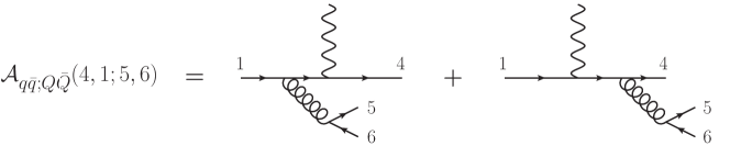
Figure 1: Master amplitude for the $q(p_{1})+e(p_{2})\to e(p_{3})+q(p_{4})+Q(p_{5})+\bar{Q}(p_{6})$ processes. The electron line is omitted. See text for details.

We consider the double-real contribution. Schematically, we write

$$\begin{split}&{{\rm d}\hat{\sigma}}^{\rm RR}_{q}\sim\\ &\int\prod_{i=3}^{6}[df_{i}]\left\{\sum_{q_{i}\neq q}|\mathcal{A}(1_{q},4_{q},5_{q_{i}},6_{{\bar{q}}_{i}})|^{2}+\frac{1}{2!}|\mathcal{A}(1_{q},4_{q},5_{q},6_{{\bar{q}}})|^{2}+\frac{1}{2!}|\mathcal{A}(1_{q},4_{q},5_{g},6_{g})|^{2}\right\}.\end{split}$$ (3.2)

We note that scattering amplitudes that involve an additional quark-anti-quark pair can be constructed from the “master” amplitude $\mathcal{A}_{q{\bar{q}};Q{\bar{Q}}}$ shown in Fig. 1. For example, the amplitude for the process $q(p_{1})+e(p_{2})\to e(p_{3})+q(p_{4})+q^{\prime}(p_{5})+{\bar{q}}^{\prime}(p_{6})$ with $q\neq q^{\prime}$ is given by

$$\mathcal{A}(1_{q},4_{q},5_{q^{\prime}},6_{{\bar{q}}^{\prime}})=\mathcal{A}_{q{\bar{q}};Q{\bar{Q}}}(4_{q},1_{q};5_{q^{\prime}},6_{{\bar{q}}^{\prime}})+\mathcal{A}_{q{\bar{q}};Q{\bar{Q}}}(5_{q^{\prime}},6_{{\bar{q}}^{\prime}};4_{q},1_{q}),$$ (3.3)

and the amplitude for the process $q(p_{1})+e(p_{2})\to e(p_{3})+q(p_{4})+q(p_{5})+{\bar{q}}(p_{6})$ is then given by

$$\mathcal{A}(1_{q},4_{q},5_{q},6_{{\bar{q}}})=\mathcal{A}(1_{q},4_{q},5_{q^{\prime}},6_{{\bar{q}}^{\prime}})+\mathcal{A}(1_{q},5_{q},4_{q^{\prime}},6_{{\bar{q}}^{\prime}}).$$ (3.4)

By systematically re-labeling partons, it is straightforward to re-write ${{\rm d}\hat{\sigma}}^{\rm RR}_{q}$ Eq. (3.2) in terms of the amplitude $\mathcal{A}_{q{\bar{q}};Q{\bar{Q}}}$ as

$$\begin{split}{{\rm d}\hat{\sigma}}^{\rm RR}_{q}&\sim\int\prod_{i=3}^{6}[df_{i}]\Bigg{\{}\sum_{q_{i}}\left[|\mathcal{A}_{q{\bar{q}};Q{\bar{Q}}}(4_{q_{i}},6_{{\bar{q}}_{i}};5_{q},1_{q})|^{2}+|\mathcal{A}_{q{\bar{q}};Q{\bar{Q}}}(4_{q},1_{q};5_{q_{i}},6_{{\bar{q}}_{i}})|^{2}\right]\\ &\quad+\frac{1}{2!}|\mathcal{A}(1_{q},4_{q},5_{g},6_{g})|^{2}+\sum_{q_{i}}2\Re\big{[}\mathcal{A}_{q{\bar{q}};Q{\bar{Q}}}(5_{q_{i}},6_{{\bar{q}}_{i}};4_{q},1_{q})\mathcal{A}^{*}_{q{\bar{q}};Q{\bar{Q}}}(4_{q},1_{q};5_{q_{i}},6_{{\bar{q}}_{i}})\big{]}\\ &\quad+\frac{2\Re}{2!}\bigg{[}\mathcal{A}_{q{\bar{q}};Q{\bar{Q}}}(5_{q},1_{q};4_{q},6_{\bar{q}})\left[\mathcal{A}^{*}_{q{\bar{q}};Q{\bar{Q}}}(4_{q},1_{q};5_{q},6_{\bar{q}})+\mathcal{A}^{*}_{q{\bar{q}};Q{\bar{Q}}}(4_{q},6_{\bar{q}};5_{q},1_{q})\right]\\ &\qquad+\mathcal{A}_{q{\bar{q}};Q{\bar{Q}}}(5_{q},6_{{\bar{q}}};4_{q},1_{\bar{q}})\left[\mathcal{A}^{*}_{q{\bar{q}};Q{\bar{Q}}}(4_{q},6_{{\bar{q}}};5_{q},1_{q})+\mathcal{A}^{*}_{q{\bar{q}};Q{\bar{Q}}}(5_{q},1_{q};4_{q},6_{{\bar{q}}})\right]\bigg{]}\Bigg{\}}.\end{split}$$ (3.5)

We stress that, contrary to Eq. (3.2), the sums in Eq. (3.5) run over all quark flavors.

It is conventional to split the real-emission processes into non-singlet, singlet and the interference contributions. To that end, we write

$${{\rm d}\hat{\sigma}}^{\rm RR}_{q}={{\rm d}\hat{\sigma}}^{\rm RR}_{q,\rm ns}+{{\rm d}\hat{\sigma}}^{\rm RR}_{q,\rm s}+{{\rm d}\hat{\sigma}}^{\rm RR}_{q,\rm int}.$$ (3.6)

The individual contributions in Eq. (3.6) are written as integrals of the corresponding amplitudes squared

$${{\rm d}\hat{\sigma}}^{\rm RR}_{q,\rm ns,s,int}\sim\int\prod_{i=3}^{6}[df_{i}]\;|\mathcal{A}_{\rm ns,s,int}(1,4,5,6)|^{2}.$$ (3.7)

These amplitudes read

$$\begin{split}&|\mathcal{A}_{\rm ns}(1,4,5,6)|^{2}=\frac{1}{2!}|\mathcal{A}(1_{q},4_{q},5_{g},6_{g})|^{2}+\sum_{q_{i}}|\mathcal{A}_{q{\bar{q}};Q{\bar{Q}}}(4_{q},1_{q};5_{q_{i}},6_{{\bar{q}}_{i}})|^{2}\\ &\quad+\frac{2\Re}{2!}\bigg{[}\mathcal{A}_{q{\bar{q}};Q{\bar{Q}}}(5_{q},1_{q};4_{q},6_{\bar{q}})\left[\mathcal{A}^{*}_{q{\bar{q}};Q{\bar{Q}}}(4_{q},1_{q};5_{q},6_{\bar{q}})+\mathcal{A}^{*}_{q{\bar{q}};Q{\bar{Q}}}(4_{q},6_{\bar{q}};5_{q},1_{q})\right]\\ &\qquad+\mathcal{A}_{q{\bar{q}};Q{\bar{Q}}}(5_{q},6_{{\bar{q}}};4_{q},1_{\bar{q}})\left[\mathcal{A}^{*}_{q{\bar{q}};Q{\bar{Q}}}(4_{q},6_{{\bar{q}}};5_{q},1_{q})+\mathcal{A}^{*}_{q{\bar{q}};Q{\bar{Q}}}(5_{q},1_{q};4_{q},6_{{\bar{q}}})\right]\bigg{]},\\ &|\mathcal{A}_{\rm s}(1,4,5,6)|^{2}=\sum_{q_{i}}|\mathcal{A}_{q{\bar{q}};Q{\bar{Q}}}(4_{q_{i}},6_{{\bar{q}}_{i}};5_{q},1_{q})|^{2},\\ &|\mathcal{A}_{\rm int}(1,4,5,6)|^{2}=\sum_{q_{i}}2\Re\big{[}\mathcal{A}_{q{\bar{q}};Q{\bar{Q}}}(5_{q_{i}},6_{{\bar{q}}_{i}};4_{q},1_{q})\mathcal{A}^{*}_{q{\bar{q}};Q{\bar{Q}}}(4_{q},1_{q};5_{q_{i}},6_{{\bar{q}}_{i}})\big{]}.\end{split}$$ (3.8)

The different contributions have a distinct structure of infra-red and collinear singularities. The strongest singularities are present in the non-singlet contribution $|\mathcal{A}_{\rm ns}|^{2}$ which exhibits non-vanishing soft and collinear singular limits. More specifically, $|\mathcal{A}(1_{q},4_{q},5_{g},6_{g})|^{2}$ is singular if either one or both gluons are soft, or when they are collinear to quarks $q_{1,4}$ or to each other. Other contributions to the non-singlet amplitude squared are less singular. For example, $|\mathcal{A}_{q{\bar{q}};Q{\bar{Q}}}(4_{q},1_{q};5_{q_{i}},6_{{\bar{q}}_{i}})|^{2}$ is singular when quarks $q_{5}$ and $q_{6}$ are both soft, or when they are collinear to each other, or when they are simultaneously collinear to $q_{1}$ or $q_{4}$.

The singlet contribution $|\mathcal{A}_{\rm s}|^{2}$ only contains collinear singularities. Double-collinear singularities arise when $q_{5}$ is collinear to $q_{1}$ or when ${\bar{q}}_{6}$ is collinear to $q_{4}$. Triple-collinear singularities arise when $q_{1},q_{5}$ and ${\bar{q}}_{6}$ are collinear or when $q_{1},q_{4}$ and $q_{5}$ are collinear. The pure interference contribution $|\mathcal{A}_{\rm int}|^{2}$ is finite. Furthermore, for photon-mediated DIS, that we consider in this paper, the integral of this contribution vanishes due to Furry’s theorem.

Since double-virtual and real-virtual corrections only contribute to the non-singlet cross section, we write

$${{\rm d}\hat{\sigma}}^{\rm NNLO}_{q}={{\rm d}\hat{\sigma}}^{\rm NNLO}_{q,\rm ns}+{{\rm d}\hat{\sigma}}^{\rm NNLO}_{q,\rm s}+{{\rm d}\hat{\sigma}}^{\rm NNLO}_{q,\rm int},$$ (3.9)

where the three terms on the right hand side, defined as

$$\begin{split}&{{\rm d}\hat{\sigma}}^{\rm NNLO}_{q,\rm ns}={{\rm d}\hat{\sigma}}^{\rm RR}_{q,\rm ns}+{{\rm d}\hat{\sigma}}^{\rm RV}_{q}+{{\rm d}\hat{\sigma}}^{\rm VV}_{q}+{{\rm d}\hat{\sigma}}^{\rm PDF}_{q,\rm ns},\\ &{{\rm d}\hat{\sigma}}^{\rm NNLO}_{q,\rm s}={{\rm d}\hat{\sigma}}^{\rm RR}_{q,\rm s}+{{\rm d}\hat{\sigma}}^{\rm PDF}_{q,\rm s},\\ &{{\rm d}\hat{\sigma}}^{\rm NNLO}_{q,\rm int}={{\rm d}\hat{\sigma}}^{\rm RR}_{q,\rm int},\end{split}$$ (3.10)

are separately finite. The collinear renormalization counterterms in Eq. (3.10) are explicitly given by

$$\begin{split}{{\rm d}\hat{\sigma}}_{q,\rm ns}^{\rm PDF}&=\left[{\frac{\alpha_{s}(\mu)}{2\pi}}\right]^{2}{{\rm d}\hat{\sigma}}_{q}^{\rm LO}\otimes\left[\frac{{\hat{P}}^{(1)}_{qq,V}+{\hat{P}}^{(1)}_{q{\bar{q}},V}}{2\epsilon}-\frac{{\hat{P}}^{(0)}_{qq}\otimes{\hat{P}}^{(0)}_{qq}+\beta_{0}{\hat{P}}^{(0)}_{qq}}{2\epsilon^{2}}\right]\\ &+\left[{\frac{\alpha_{s}(\mu)}{2\pi}}\right]{{\rm d}\hat{\sigma}}_{q}^{\rm NLO}\otimes{\hat{P}}^{(0)}_{qq};\\ {{\rm d}\hat{\sigma}}_{q,\rm s}^{\rm PDF}&=\left[{\frac{\alpha_{s}(\mu)}{2\pi}}\right]^{2}{{\rm d}\hat{\sigma}}^{\rm LO}_{q}\otimes\left[\frac{{\hat{P}}^{(1)}_{qq,\rm s}}{2\epsilon}-\frac{{\hat{P}}^{(0)}_{qg}\otimes{\hat{P}}^{(0)}_{gq}}{2\epsilon^{2}}\right]+\left[{\frac{\alpha_{s}(\mu)}{2\pi}}\right]{{\rm d}\hat{\sigma}}^{\rm NLO}_{g}\otimes{\hat{P}}^{(0)}_{gq}.\end{split}$$ (3.11)

As usual, the sign “$\otimes$” stands for the convolution product and ${\hat{P}}^{(0/1)}$ are leading and next-to-leading order Altarelli-Parisi splitting functions, see e.g. [43]. We report them in Appendix A for convenience. The leading-order QCD $\beta$ function, which appears in Eq. (3.11), reads

$$\beta_{0}=\frac{11}{6}{C_{A}}-\frac{2}{3}{T_{R}}{n_{f}},$$ (3.12)

where ${C_{A}}=3$, ${T_{R}}=1/2$ and $n_{f}$ is a number of massless quark flavors.

3.1.1 NNLO corrections in the non-singlet channel: derivation

The goal of this section is to describe the calculation of NNLO QCD corrections to neutral current DIS in the non-singlet channel. Our goal in this discussion is two-fold. On the one hand, we aim to show that many ingredients of the current computation are similar to cases of color-singlet production and decay discussed in Refs. [1, 2, 3] and, for this reason, can be directly borrowed from these references. On the other hand, we want to emphasize new elements required for the construction of the nested subtraction scheme when a process involves color-charged initial- and final-state partons.

We start by discussing the double-real contribution ${{\rm d}\hat{\sigma}}^{\rm RR}_{q,\rm ns}$. It contains double-soft singularities which arise when partons $f_{5,6}$ become soft, $E_{5}\sim E_{6}\to 0$. Because of this, we find it convenient to order energies of partons $f_{5,6}$, see Ref. [1]. Using the notation of Section 2, we then define

$$\begin{split}&\left\langle F_{\rm LM,ns}(1,4,5,6)\mathcal{O}(\{1,...,6\})\right\rangle\equiv\mathcal{N}\int\prod_{i=3}^{6}[df_{i}]\;(2\pi)^{d}\delta^{(d)}\left(p_{1}+p_{2}-\sum_{i=3}^{6}p_{i}\right)\\ &\quad\times\theta(E_{5}-E_{6})\bigg{[}|\mathcal{A}_{\rm ns}(1,4,5,6)|^{2}+|\mathcal{A}_{\rm ns}(1,4,6,5)|^{2}\bigg{]}\mathcal{O}(\{p_{1},...,p_{6}\}),\end{split}$$ (3.13)

so that

$$2s\cdot{{\rm d}\hat{\sigma}}^{\rm RR}_{\rm ns}=\left\langle F_{\rm LM,ns}(1,4,5,6)\right\rangle_{\delta}.$$ (3.14)

To extract soft and collinear singularities from $F_{\rm LM,ns}(1,4,5,6)$, we closely follow the procedure described in Refs. [1, 2, 3].

First, we extract the double soft $E_{5}\sim E_{6}\to 0$ singularity. Similar to Refs. [1, 2, 3], we introduce an operator $\SS$ that extracts the leading soft behavior of the matrix element, and sets $E_{5,6}$ to zero in both the momentum-conserving $\delta$-function and the observable $\mathcal{O}$ in Eq. (3.13). We write

$$\left\langle F_{\rm LM,ns}(1,4,5,6)\right\rangle_{\delta}=\left\langle\SS F_{\rm LM,ns}(1,4,5,6)\right\rangle+\left\langle(I-\SS)F_{\rm LM,ns}(1,4,5,6)\right\rangle_{\delta}.$$ (3.15)

The second term on the r.h.s. of Eq. (3.15) is free of double-soft singularities. In the first term, partons $f_{5,6}$ completely decouple from the hard matrix element and any infra-red safe observable. Explicitly, we have

$$\left\langle\SS F_{\rm LM,ns}(1,4,5,6)\right\rangle=\left\langle\left[g_{s,b}^{4}\int[df_{5}][df_{6}]{\rm Eik}(1,4;5,6)\right]F_{\rm LM}(1_{q},4_{q})\right\rangle_{\delta},$$ (3.16)

where the function Eik(1,4;5,6) is the square of the double eikonal currents computed e.g. in Ref. [44]. Compared to the color-singlet production and decay cases described in Refs. [1, 2, 3], the integral of ${\rm Eik}(1,4;5,6)$ depends on the relative angle between directions of hard partons $f_{1,4}$. This integral was computed in Ref. [5] for a generic opening angle between $f_{1}$ and $f_{4}$, so we can directly take the result from there.

The second term on the l.h.s. of Eq. (3.15) is free from the double-soft singularity, but still contains single-soft $E_{6}\to 0$ singularity. To extract it, we use $I=S_{6}+(I-S_{6})$ and write

$$\begin{split}&\left\langle(I-\SS)F_{\rm LM,ns}(1,4,5,6)\right\rangle_{\delta}\\ &=\left\langle S_{6}(I-\SS)F_{\rm LM,ns}(1,4,5,6)\right\rangle+\left\langle(I-S_{6})(I-\SS)F_{\rm LM,ns}(1,4,5,6)\right\rangle_{\delta}.\end{split}$$ (3.17)

We deal with the first term on the right hand side of Eq. (3.17) following the discussion of the NLO computation, c.f. Eq. (2.20). The only differences with respect to that case are $a)$ a more involved color structure and $b)$ the maximal allowed energy of $f_{6}$ is now $E_{5}$, because of the energy ordering. Taking into account that the $S_{6}$ singularity is only present if parton $f_{6}$ is a gluon, we obtain

$$\begin{split}&\left\langle S_{6}(I-\SS)F_{\rm LM,ns}(1,4,5,6)\right\rangle\\[5.0pt] &=\frac{{[\alpha_{s}]}^{2}}{\epsilon^{2}}\Bigg{\langle}\left(\frac{4E_{5}^{2}}{\mu^{2}}\right)^{-\epsilon}\bigg{[}(2{C_{F}}-{C_{A}})\eta_{41}^{-\epsilon}K_{14}+{C_{A}}\big{[}\eta_{51}^{-\epsilon}K_{15}+\eta_{54}^{-\epsilon}K_{54}\big{]}\bigg{]}\\ &\quad\times(I-S_{5})F_{\rm LM}(1_{q},4_{q},5_{g})\bigg{\rangle}_{\delta}.\end{split}$$ (3.18)

The right-hand side in Eq. (3.18) still contains unregulated singularities that arise when $g_{5}$ is collinear to $q_{1}$ or $q_{4}$. To extract them, we proceed as in the NLO case. To this end, we again use the partition of unity shown in Eq. (2.11) and write

$$I=\sum_{i\in[1,4]}(I-C_{5i})w^{5i}+\sum_{i}C_{5i},$$ (3.19)

where we used $C_{5i}w^{5j}=\delta_{ij}$. When Eq. (3.19) is used in Eq. (3.18), the first term on the right hand side of Eq. (3.19) leads to a fully-regulated contribution, while the second term extracts the collinear divergences. Its integration over the unresolved phase space proceeds similar to the NLO case except for two differences.

• When compared to NLO calculations, Eq. (3.18) contains an additional $E_{5}^{-2\epsilon}$ factor. This leads to modified powers of $(1-z)^{-2\epsilon}$ in collinear limits of differential cross sections. To efficiently deal with this case, we find it convenient to define a generalised version of Eq. (2.33). It reads

  $$\begin{split}&{\mathcal{P}}_{qq,Rn}(z)\equiv 2{C_{F}}\left[\frac{(1-z)^{-n\epsilon}}{1-z}\right]_{+}+(1-z)^{-n\epsilon}P_{qq,\rm reg}(z),\\ &\gamma_{qq}^{nk}\equiv-\int\limits_{0}^{1}{\rm d}z\left[z^{-n\epsilon}(1-z)^{-k\epsilon}P_{qq}(z)-\frac{2{C_{F}}}{(1-z)^{1+k\epsilon}}\right],\end{split}$$ (3.20)

  where $P_{qq}$ is the splitting function defined in Eq. (2.25).

• The pre-factor in Eq. (3.18) leads to terms of the form $C_{ij}\left[\eta_{ij}^{-\epsilon}K_{ij}\right]$. This slightly changes the angular integral that needs to be computed. This point was already discussed in Refs. [1, 2, 3], and we refer the reader to these references for details.

Taking into account these two differences, and repeating steps explained in the context of the NLO calculation, we obtain

$$\begin{split}&\left\langle C_{51}S_{6}(I-\SS)F_{\rm LM,ns}(1,4,5,6)\right\rangle=-\frac{{[\alpha_{s}]}^{2}}{\epsilon^{3}}\int\limits_{0}^{1}{\rm d}z\\ &\quad\times\Bigg{\langle}\Bigg{[}-\left(\frac{4E_{1}^{2}}{\mu^{2}}\right)^{-2\epsilon}{\mathcal{P}}_{qq,R4}(z)+2{C_{F}}\left[\frac{(4E_{1}^{2}/\mu^{2})^{-2\epsilon}-(4E_{\rm max}^{2}/\mu^{2})^{-2\epsilon}}{4\epsilon}\right]\delta(1-z)\Bigg{]}\\ &\qquad\times\left[-2{C_{F}}\frac{\Gamma^{2}(1-\epsilon)}{\Gamma(1-2\epsilon)}\eta_{41}^{-\epsilon}K_{14}-\frac{{C_{A}}}{2}\frac{\Gamma^{4}(1-\epsilon)\Gamma(1+\epsilon)}{\Gamma(1-3\epsilon)}\right]\frac{F_{\rm LM}(z\cdot 1_{q},4_{q})}{z}\Bigg{\rangle}_{\delta},\end{split}$$ (3.21)

for initial-state singularities, and

$$\begin{split}&\left\langle C_{54}S_{6}(I-\SS)F_{\rm LM,ns}(1,4,5,6)\right\rangle\\ &=-\frac{{[\alpha_{s}]}^{2}}{\epsilon^{3}}\Bigg{\langle}\Bigg{[}\left(\frac{4E_{3}^{2}}{\mu^{2}}\right)^{-2\epsilon}\gamma_{qq}^{24}+2{C_{F}}\left[\frac{(4E_{3}^{2}/\mu^{2})^{-2\epsilon}-(4E_{\rm max}^{2}/\mu^{2})^{-2\epsilon}}{4\epsilon}\right]\Bigg{]}\\ &\quad\times\left[-2{C_{F}}\frac{\Gamma^{2}(1-\epsilon)}{\Gamma(1-2\epsilon)}\eta_{41}^{-\epsilon}K_{14}-\frac{{C_{A}}}{2}\frac{\Gamma^{4}(1-\epsilon)\Gamma(1+\epsilon)}{\Gamma(1-3\epsilon)}\right]F_{\rm LM}(1_{q},4_{q})\Bigg{\rangle}_{\delta},\end{split}$$ (3.22)

for final-state ones.

Combining the various terms discussed above, we arrive at the following formula

$$\left\langle F_{\rm LM,ns}(1,4,5,6)\right\rangle_{\delta}=\left\langle(I-S_{6})(I-\SS)F_{\rm LM,ns}(1,4,5,6)\right\rangle_{\delta}+...$$ (3.23)

where ellipses stand for various contributions from which all soft and collinear singularities have been extracted, as described above. However, the first term on the right hand side of Eq. (3.23) still contains unregulated collinear singularities. To proceed with their extraction, we follow the FKS approach [40, 41] and its NNLO extension [10], and partition the phase space in the following way

$$1=w^{51,61}+w^{54,64}+w^{51,64}+w^{54,61},$$ (3.24)

where $w^{5i,6j}$ are designed to dampen all but a few collinear singularities. More specifically, we ask that the damping factors behave in the following way:

$$C_{5i}w^{5j,6k}\propto\delta_{ij},~{}~{}~{}C_{6i}w^{5j,6k}\propto\delta_{ik};~{}~{}~{}i,j,k\in[1,4].$$ (3.25)

We also find it convenient to construct the functions $w^{5i,6j}$ in such a way that $w^{51,64}$ and $w^{54,61}$ vanish in the limit when $f_{5}$ and $f_{6}$ become collinear to each other and that they are symmetric under the $5\leftrightarrow 6$ exchange. Apart from these requirements, the explicit form of the damping factors is mostly immaterial. An explicit construction of these factors, valid also for the DIS case, was discussed in Ref. [1, 2, 3]. We report it in Appendix B for convenience.

In the “double-collinear” partitions $w^{51,64}$, $w^{54,61}$, collinear singularities are effectively NLO-like. In the “triple-collinear” partitions $w^{51,61}$ and $w^{54,64}$ genuine triple-collinear singularities occur when partons $f_{5,6}$ become collinear to $f_{1}$ or $f_{4}$, respectively. However, since these triple-collinear limits can be reached in a variety of ways, it is useful to introduce additional angular ordering to isolate physically-inequivalent configurations [10]. For the partition $w^{5i,6i}$, we write

$$\begin{split}w^{5i,6i}&=w^{5i,6i}\left(\theta\left(\rho_{6i}<\frac{\rho_{5i}}{2}\right)+\theta\left(\frac{\rho_{5i}}{2}<\rho_{6i}<\rho_{5i}\right)+(5\leftrightarrow 6)\right)\\ &\equiv w^{5i,6i}\left(\theta_{i}^{(a)}+\theta_{i}^{(b)}+\theta_{i}^{(c)}+\theta_{i}^{(d)}\right).\end{split}$$ (3.26)

We note in passing that the angular ordering Eq. (3.26) can also be enforced by constructing appropriate damping factors [23]. Nevertheless, we find it practical to employ Eq. (3.26) to isolate and extract collinear singularities and to integrate the subtraction terms analytically. In particular, a phase space parametrization that naturally implements the sector decomposition as in Eq. (3.26) and that we employ in this paper can be found in Ref. [10].

We extract the remaining collinear singularities using Eqs. (3.24,3.26). To this end, we follow Refs. [1, 2, 3] and write

$$\begin{split}&\left\langle(I-S_{6})(I-\SS)F_{\rm LM,ns}(1,4,5,6)\right\rangle_{\delta}\\ &=\left\langle F_{\rm LM,ns}^{s_{r}c_{s}}(1,4,5,6)\right\rangle+\left\langle F_{\rm LM,ns}^{s_{r}c_{t}}(1,4,5,6)\right\rangle+\left\langle F_{\rm LM,ns}^{s_{r}c_{r}}(1,4,5,6)\right\rangle_{\delta}.\end{split}$$ (3.27)

The three terms on the right hand side in Eq. (3.27) are defined as follows:

• the soft-regulated single-collinear contribution $F_{\rm LM,ns}^{s_{r}c_{s}}$ reads

  $$\begin{split}&\left\langle F_{\rm LM,ns}^{s_{r}c_{s}}(1,4,5,6)\right\rangle\\ &=\sum_{(ij)\in[14,41]}\bigg{\langle}\bigg{[}C_{5i}[df_{5}]+C_{6j}[df_{6}]\bigg{]}w^{5i,6j}(I-S_{6})(I-\SS)\times F_{\rm LM,ns}(1,4,5,6)\bigg{\rangle}\\ &+\sum_{i\in[1,4]}\bigg{\langle}\bigg{[}\theta^{(a)}C_{6i}+\theta^{(b)}C_{56}+\theta^{(c)}C_{5i}+\theta^{(d)}C_{56}\bigg{]}\\ &\qquad\times[df_{5}][df_{6}]\;w^{5i,6i}(I-S_{6})(I-\SS)F_{\rm LM,ns}(1,4,5,6)\bigg{\rangle},\end{split}$$ (3.28)

• the soft-regulated triple- and double-collinear contribution $F_{\rm LM,ns}^{s_{r}c_{s}}$ reads

  $$\begin{split}&\left\langle F_{\rm LM,ns}^{s_{r}c_{t}}(1,4,5,6)\right\rangle\\ &=\sum_{i\in[1,4]}\bigg{\langle}\bigg{[}\theta^{(a)}(I-C_{6i})+\theta^{(b)}(I-C_{65})+\theta^{(c)}(I-C_{5i})+\theta^{(d)}(I-C_{65})\bigg{]}\\ &\quad\times[df_{5}][df_{6}]\;C{C}_{i}w^{5i,6i}(I-S_{6})(I-\SS)F_{\rm LM,ns}(1,4,5,6)\bigg{\rangle}\\ &-\sum_{(ij)\in[14,41]}\left\langle C_{5i}C_{6j}[df_{5}][df_{6}]w^{5i,6j}(I-S_{6})(I-\SS)F_{\rm LM,ns}(1,4,5,6)\right\rangle,\end{split}$$ (3.29)

• and, finally, the fully-regulated term reads

  $$\begin{split}&\left\langle F_{\rm LM,ns}^{s_{r}c_{r}}(1,4,5,6)\right\rangle_{\delta}\\ &=\sum_{i\in[1,4]}\bigg{\langle}\bigg{[}\theta^{(a)}(I-C_{6i})+\theta^{(b)}(I-C_{65})+\theta^{(c)}(I-C_{5i})+\theta^{(d)}(I-C_{65})\bigg{]}\\ &\quad\times[df_{5}][df_{6}]\;(I-C{C}_{i})w^{5i,6i}(I-S_{6})(I-\SS)F_{\rm LM,ns}(1,4,5,6)\bigg{\rangle}_{\delta}\\ &+\sum_{(ij)\in[14,41]}\bigg{\langle}\bigg{[}(I-C_{5i})(I-C_{6j})\bigg{]}[df_{5}][df_{6}]\;(I-S_{6})(I-\SS)F_{\rm LM,ns}(1,4,5,6)\bigg{\rangle}_{\delta}.\end{split}$$ (3.30)

We note that in Eqs. (3.28,3.29,3.30) we used the notation introduced in Refs. [1, 2, 3]. In particular, $C{C}_{i}$ denote triple-collinear limits, and collinear operators act on everything that appears to the right of them. For example, by writing $C_{ij}[df_{j}]$ we indicate that the phase space for parton $j$ has to be taken in the corresponding collinear limit, see Refs. [1, 2, 3] for details.

A detailed discussion of double- and triple-collinear sectors, both for initial- and final-state collinear singularities, can be found in Refs. [2, 3]. The fact that the discussion of these limits does not change is the consequence of the fact that collinear singularities only depend on color charges and types of external partons; as the result, once the production and decay of color singlets are understood, the description of similar limits in DIS naturally follows. For this reason we do not repeat the discussion of collinear limits per se but, instead, illustrate new features that arise in the DIS case by focusing on a few representative examples.

We start by discussing the contribution shown in Eq. (3.29). Compared to the cases studied in Refs. [2, 3], the collinear limits now have an explicit $E_{\rm max}$ dependence. For the triple-collinear limits, relevant results were obtained in Ref. [4], and we refer the reader to this reference for details. For the double-collinear case, we need to evaluate

$$\begin{split}\mathcal{DC}=-\left\langle\big{[}C_{51}C_{64}+C_{54}C_{61}\big{]}[df_{5}][df_{6}](I-S_{6})(I-\SS)F_{\rm LM,ns}(1,4,5,6)\right\rangle.\end{split}$$ (3.31)

In the non-singlet channel, $\mathcal{DC}$ is non-vanishing only if both partons 5 and 6 are gluons. Schematically, Eq. (3.31) reads

$$\begin{split}&\big{[}C_{51}C_{64}+C_{54}C_{61}\big{]}[df_{5}][df_{6}]\;(I-S_{6})(I-\SS)F_{\rm LM,ns}(1,4,5,6)\\ &\sim\big{[}C_{51}C_{64}+C_{54}C_{61}\big{]}[df_{5}][df_{6}]\;\theta(E_{5}-E_{6})\theta(E_{\rm max}-E_{5})(I-S_{6})(I-\SS)\\ &\quad\times\left[|\mathcal{A}^{\rm tree}|^{2}(1_{q},2_{e},3_{e},4_{q},5_{g},6_{g})[df_{4}]\;(2\pi)^{d}\delta^{(d)}\left(p_{1}+p_{2}-\sum_{i=3}^{6}p_{i}\right)\right].\end{split}$$ (3.32)

We note that apart from the operator $S_{6}$ and the energy-ordering condition, this expression is symmetric under the exchange $f_{5}\leftrightarrow f_{6}$. Accounting for that and renaming partons appropriately, it is easy to show that Eq. (3.32) can be written as

$$\begin{split}&\big{[}C_{51}C_{64}+C_{54}C_{61}\big{]}[df_{5}][df_{6}]\;(I-S_{6})(I-\SS)F_{\rm LM,ns}(1,4,5,6)\\ &\sim\Big{\{}C^{s_{r}}_{51}C^{s_{r}}_{64}\theta_{E_{5}<E_{\rm max}}\theta_{E_{6}<E_{\rm max}}+\big{[}C_{51}S_{5}\theta_{E_{6}<E_{5}<E_{\rm max}}\big{]}C^{s_{r}}_{64}+\big{[}C_{64}S_{6}\theta_{E_{5}<E_{6}<E_{\rm max}}\big{]}C^{s_{r}}_{51}\Big{\}}\\ &\quad\times\left[|\mathcal{A}^{\rm tree}|^{2}(1_{q},2_{e},3_{e},4_{q},5_{g},6_{g})[df_{4}][df_{5}][df_{6}]\;(2\pi)^{d}\delta^{(d)}\left(p_{1}+p_{2}-\sum_{i=3}^{6}p_{i}\right)\right],\end{split}$$ (3.33)

where we used the short-hand notations $C_{5(6)i}^{s_{r}}=C_{5(6)i}(I-S_{5(6)})$ and $\theta_{X<Y}=\theta(Y-X)$, $\theta_{X<Y<Z}=\theta(Y-X)\theta(Z-Y)$. We note that each of the three terms in the curly bracket in Eq. (3.33) does not contain unregulated soft divergences. The first term is just the product of two NLO-like contributions; for this reason, it can be immediately read off from Eqs. (2.29, 2.32). In the second term, the $C_{51}S_{5}$ soft-collinear limit leads to

$$\begin{split}&\left\langle C_{51}S_{5}\theta_{E_{6}<E_{5}<E_{\rm max}}[df_{5}]\;F_{\rm LM,ns}(1,4,5,6)\right\rangle\\[5.0pt] &=-2{C_{F}}\frac{{[\alpha_{s}]}}{\epsilon}\left(\frac{4}{\mu^{2}}\right)^{-\epsilon}\left\langle\int\limits_{E_{6}}^{E_{\rm max}}\frac{{\rm d}E_{5}}{E_{5}^{1+2\epsilon}}F_{\rm LM}(1_{q},4_{q},6_{g})\right\rangle\\ &=-2{C_{F}}\frac{{[\alpha_{s}]}}{\epsilon}\left\langle\Delta(E_{6}^{2},E_{\rm max}^{2})F_{\rm LM}(1_{q},4_{q},6_{g})\right\rangle,\end{split}$$ (3.34)

where the function $\Delta$ is defined in Eq. (2.34). According to Eq. (3.33), we now have to take the soft-regulated collinear limit $C^{s_{r}}_{64}$ of Eq. (3.34). For the term proportional to $E_{\rm max}$, everything proceeds as in the NLO case. The term proportional to $E_{6}$, however, induces an extra power of $(1-z)^{-2\epsilon}$ after performing the change of variables $E_{6}=(1-z)E_{64}$, see Eq. (2.31). As we already explained when discussing single-soft singularities, this leads to a term proportional to $\gamma_{qq}^{24}$, c.f. Eq. (3.20). More precisely, we obtain

$$\begin{split}&\left\langle C_{64}^{s_{r}}C_{51}S_{5}\theta_{E_{6}<E_{5}<E_{\rm max}}[df_{5}][df_{6}]F_{\rm LM,ns}(1,4,5,6)\right\rangle=-2{C_{F}}\frac{{[\alpha_{s}]}^{2}}{\epsilon^{2}}\\ &\quad\times\bigg{\langle}\bigg{[}\frac{(4E_{4}^{2}/\mu^{2})^{-2\epsilon}\gamma_{qq}^{24}-(4E_{4}E_{\rm max}/\mu^{2})^{-2\epsilon}\gamma_{qq}^{22}}{2\epsilon}+2{C_{F}}\frac{\Delta^{2}(E_{4}^{2},E_{\rm max}^{2})}{2}\bigg{]}F_{\rm LM}(1_{q},4_{q})\bigg{\rangle}_{\delta}.\end{split}$$ (3.35)

An analogous result can be found for the last term in the curly bracket of Eq. (3.33) that describes the regulated initial-state radiation and the soft final-state radiation.

The last double-real contribution that we need to discuss is the soft-regulated single-collinear term Eq. (3.28). Once again, an in-depth discussion of this term can be found in Refs. [2, 3], and we do not repeat it here. Rather, we illustrate the new features arising when considering the DIS process by focusing on the initial triple-collinear sectors $w^{51,61}\theta^{(a,c)}$. Once these cases are understood, generalization to other sectors does not pose conceptual challenges and can be obtained following the discussion in Refs. [2, 3]. Schematically, we write

$$\begin{split}&\bigg{[}\theta^{(a)}C_{61}+\theta^{(c)}C_{51}\bigg{]}[df_{5}][df_{6}]\;w^{51,61}(I-S_{6})(I-\SS)F_{\rm LM,ns}(1,4,5,6)\\ &\sim\bigg{[}\theta\left(\rho_{61}-\frac{\rho_{51}}{2}\right)C_{61}+\theta\left(\rho_{51}-\frac{\rho_{61}}{2}\right)C_{51}\bigg{]}w^{51,61}[df_{5}][df_{6}]\;\theta_{E_{5}<E_{6}<E_{\rm max}}\\ &\quad\times(I-S_{6})(I-\SS)\left[|\mathcal{A}^{\rm tree}|^{2}(1_{q},2_{e},3_{e},4_{q},5_{g},6_{g})[df_{4}]\;(2\pi)^{d}\delta^{(d)}\left(p_{1}+p_{2}-\sum_{i=3}^{6}p_{i}\right)\right],\end{split}$$ (3.36)

where we used the fact that in the non-singlet channel the $C_{51}$ and $C_{61}$ limits are only singular if both partons 5 and 6 are gluons. To proceed further, we follow the discussion of the double-collinear contribution. We use the symmetry of $F_{\rm LM,ns}$ with respect to an interchange of $g_{5}$ and $g_{6}$ and re-write Eq. (3.36) as

$$\begin{split}&\bigg{[}\theta^{(a)}C_{61}+\theta^{(c)}C_{51}\bigg{]}[df_{5}][df_{6}]\;w^{51,61}(I-S_{6})(I-\SS)F_{\rm LM,ns}(1,4,5,6)\\ &\sim\Bigg{\{}\bigg{[}C_{61}\big{[}I\cdot\theta_{E_{5}<E_{\rm max}}\theta_{E_{6}<E_{\rm max}}-S_{6}\theta_{E_{6}<E_{5}<E_{\rm max}}\big{]}\bigg{]}(I-S_{5})\\ &\qquad+\big{[}C_{61}(I-S_{6})\big{]}\big{[}S_{5}\theta_{E_{6}<E_{5}<E_{\rm max}}\big{]}\Bigg{\}}w^{51,61}[df_{5}][df_{6}]\;\theta\left(\rho_{61}<\frac{\rho_{51}}{2}\right)\\ &\quad\times\left[|\mathcal{A}^{\rm tree}|^{2}(1_{q},2_{e},3_{e},4_{q},5_{g},6_{g})[df_{4}]\;(2\pi)^{d}\delta^{(d)}\left(p_{1}+p_{2}-\sum_{i=3}^{6}p_{i}\right)\right].\end{split}$$ (3.37)

We now analyze the two terms in the curly bracket. We note that both of them only contain collinear divergences. Indeed, the soft singularity is always regulated, either by the explicit subtraction, as in the first term, or by the energy-ordering condition, as in the second one.

It is easy to see that the structure of the first term in Eq. (3.37) is nearly identical to the NLO case except that in the soft-collinear limit the upper bound on the energy of the parton $f_{6}$ is $E_{5}$ (contrary to $E_{\rm max}$ in the NLO case). This observation allows us to immediately write the result for this contribution following the discussion in Section 2. We find

$$\begin{split}&\bigg{[}C_{61}\big{[}I\cdot\theta_{E_{5}<E_{\rm max}}\theta_{E_{6}<E_{\rm max}}-S_{6}\theta_{E_{6}<E_{5}<E_{\rm max}}\big{]}\bigg{]}(I-S_{5})\longrightarrow\\ &\quad\frac{{[\alpha_{s}]}}{\epsilon}\int\limits_{0}^{1}{\rm d}z\bigg{\langle}\bigg{[}-\left(\frac{4E_{1}^{2}}{\mu^{2}}\right)^{-\epsilon}{\mathcal{P}}_{qq,R2}(z)+2{C_{F}}\Delta(E_{1}^{2},E_{5}^{2})\delta(1-z)\bigg{]}\\ &\qquad\times{\widetilde{w}}^{51,61}_{6||1}\left(\frac{\rho_{51}}{2}\right)^{-\epsilon}(I-S_{5})\frac{F_{\rm LM}(z\cdot 1_{q},4_{q},5_{g})}{z}\bigg{\rangle}.\end{split}$$ (3.38)

We note that functions ${\mathcal{P}}_{qq,R2}$ and $\Delta$, that appear in Eq. (3.38), are defined in Eqs. (3.20) and (2.34), respectively. Also, with ${\widetilde{w}}$, we indicate the damping factor in the collinear limit, i.e.

$${\widetilde{w}}^{5i,6j}_{6||k}=\lim_{\rho_{6k}\to 0}w^{5i,6j}.$$ (3.39)

Finally, we note that the factor $(\rho_{51}/2)^{-\epsilon}$, which is not present in the NLO case, arises from the ordering condition $\theta(\rho_{61}<\rho_{51}/2)$ in Eq. (3.37).

Eq. (3.38) still contains an unregulated collinear singularity that occurs when $g_{5}$ and $q_{1}$ become collinear. We extract it in the usual way by inserting $I=C_{51}+(I-C_{51})$. The regularization of the term proportional to ${\mathcal{P}}_{qq}$ was explained in detail in Ref. [2]. The regularization of the term proportional to $\Delta$ is analogous to what we just discussed for the double-collinear contribution.

We then move to the second term in curly brackets of Eq. (3.37), which corresponds to the nested soft-collinear limit. Since in the limit when $g_{6}$ is collinear to $q_{1}$, the emission of the soft gluon $g_{5}$ can not resolve $g_{6}$ and $q_{1}$, we are allowed to write

$$\begin{split}&S_{5}C_{61}(I-S_{6})w^{51,61}|\mathcal{A}(1_{q},2_{e},3_{e},4_{q},5_{g},6_{g})|^{2}\\ &=g^{2}_{s,b}\frac{2{C_{F}}}{E_{5}^{2}}\frac{\rho_{14}}{\rho_{51}\rho_{54}}{\widetilde{w}}^{51,61}_{6||1}C_{61}(I-S_{6})|\mathcal{A}(1_{q},2_{e},3_{e},4_{q},6_{g})|^{2}.\end{split}$$ (3.40)

Similar to the NLO case, the dependence on the momentum of gluon $g_{5}$ has disappeared from the hard matrix element. However, a residual dependence on $p_{5}$ in ${\widetilde{w}}^{51,61}_{6||1}$ and in the pre-factor $(\rho_{51}/2)^{-\epsilon}$ appeared. The dependence on the kinematics of gluon $g_{5}$ is described by the following integral

$$\begin{split}&g_{s,b}^{2}\int\limits_{E_{6}}^{E_{\rm max}}\frac{{\rm d}E_{5}}{E_{5}^{1+2\epsilon}}\frac{{\rm d}\Omega^{d-1}_{5}}{2(2\pi)^{d-1}}\frac{\rho_{41}}{\rho_{51}\rho_{54}}\left(\frac{\rho_{51}}{2}\right)^{-\epsilon}{\widetilde{w}}^{51,61}_{6||1}\\ &=\frac{{[\alpha_{s}]}}{\epsilon}\frac{(4E_{\rm max}^{2}/\mu^{2})^{-\epsilon}-(4E_{6}/\mu^{2})^{-\epsilon}}{2\epsilon}\left\langle\left(\frac{\rho_{51}}{2}\right)^{-\epsilon}{\widetilde{w}}^{51,61}_{6||1}\right\rangle_{S_{5}},\end{split}$$ (3.41)

where we defined

$$\left\langle\mathcal{O}\right\rangle_{S_{5}}\equiv-\epsilon\left[\frac{1}{8\pi^{2}}\frac{(4\pi)^{\epsilon}}{\Gamma(1-\epsilon)}\right]^{-1}\int\frac{{\rm d}\Omega_{5}^{d-1}}{2(2\pi)^{d-1}}\frac{\rho_{41}}{\rho_{51}\rho_{54}}\;4^{\epsilon}\;\mathcal{O}.$$ (3.42)

The contribution from the second term in the curly bracket in Eq. (3.37) is then

$$\begin{split}&\big{[}C_{61}(I-S_{6})\big{]}\big{[}S_{5}\theta_{E_{6}<E_{5}<E_{\rm max}}\big{]}\dots\longrightarrow\\ &\quad\frac{{[\alpha_{s}]}}{\epsilon}\Bigg{\langle}C_{61}(1-S_{6})[df_{6}]\;\frac{(4E_{\rm max}^{2}/\mu^{2})^{-\epsilon}-(4E_{6}/\mu^{2})^{-\epsilon}}{2\epsilon}F_{\rm LM}(1_{q},4_{q},6_{g})\\ &\qquad\times\left[2{C_{F}}\left\langle\left(\frac{\rho_{51}}{2}\right)^{-\epsilon}{\widetilde{w}}^{51,61}_{6||1}\right\rangle_{S_{5}}\right]\Bigg{\rangle}_{\delta}.\end{split}$$ (3.43)

At this stage, we can treat the collinear singularity as before. We note that the pre-factor $E_{6}^{-2\epsilon}$ will lead to additional overall factors of $(1-z)^{-\epsilon}$, as discussed above. Taking this into account and repeating steps similar to what is done in the NLO case, we obtain

$$\begin{split}&\big{[}C_{61}(I-S_{6})\big{]}\big{[}S_{5}\theta_{E_{6}<E_{5}<E_{\rm max}}\big{]}\dots\longrightarrow\\ &\quad-\frac{{[\alpha_{s}]}^{2}}{\epsilon^{2}}\int\limits_{0}^{1}{\rm d}z\;\Bigg{\langle}\bigg{[}\frac{(4E_{\rm max}E_{1}/\mu^{2})^{-2\epsilon}{\mathcal{P}}_{qq,R2}(z)-(4E_{1}^{2}/\mu^{2})^{-\epsilon}{\mathcal{P}}_{qq,R4}(z)}{2\epsilon}\\ &\qquad+2{C_{F}}\frac{\Delta^{2}(E_{1}^{2},E_{\rm max}^{2})}{2}\delta(1-z)\bigg{]}\frac{F_{\rm LM}(z\cdot 1,4)}{z}\left[2{C_{F}}\left\langle\left(\frac{\rho_{51}}{2}\right)^{-\epsilon}{\widetilde{w}}^{51,61}_{6||1}\right\rangle_{S_{5}}\right]\Bigg{\rangle}_{\delta}.\end{split}$$ (3.44)

This completes our discussion of the regularization of the triple-collinear sectors $w^{51,61}\theta^{(a,c)}$. Finally, we note that this procedure is generic and that one can regulate all the remaining sectors following it.

Before discussing the real-virtual and double-virtual contributions, we comment on the explicit dependence of Eq. (3.44) on the damping factor ${\widetilde{w}}$. In general, one expects that $1/\epsilon$ poles of the double-real contribution are independent of the damping factors, since they do not appear in any other part (double-virtual, real-virtual etc.) of the calculation. Eq. (3.44) seems to contradict this assertion. We will now show that this is not the case. To this end, we note that the sum over double-collinear partitions in Eq. (3.28) leads to a contribution which is almost identical to Eq. (3.44). The only differences in the double-collinear case with respect to Eq. (3.44) are $(a)$ the damping factor ${\widetilde{w}}^{54,61}_{6||1}$ instead of ${\widetilde{w}}^{51,61}_{6||1}$ and $(b)$ the lack of the $(\rho_{51}/2)^{-\epsilon}$ term, since we do not require angular ordering in the double-collinear partition. Taking the sum of the contributions that come from double and triple collinear partitions, we obtain the following integral

$$\left\langle\Delta_{61}\right\rangle_{S_{5}}\sim-\epsilon\int{\rm d}\Omega^{d-1}_{5}\frac{\rho_{41}}{\rho_{51}\rho_{54}}\Delta_{61},~{}~{}~{}~{}~{}\Delta_{61}={\widetilde{w}}^{54,61}_{6||1}+\left(\frac{\rho_{51}}{2}\right)^{-\epsilon}{\widetilde{w}}^{51,61}_{6||1},$$ (3.45)

see Eq. (3.42). This amounts to replacing $(\rho_{51}/2)^{-\epsilon}{\widetilde{w}}^{51,61}_{6||1}\to\Delta_{61}$ in Eq. (3.44). The term $\left\langle\Delta_{61}\right\rangle_{S_{5}}$ enters the differential cross section in the combination $\left\langle\Delta_{61}\right\rangle_{S_{5}}/\epsilon^{2}$, c.f. Eq. (3.44); this implies that we should prove that the dependence of $\left\langle\Delta_{61}\right\rangle_{S_{5}}$ on the partitioning $w$ only starts at ${\cal O}(\epsilon^{2})$.

Since the integrand in Eq. (3.45) is singular in two collinear limits $\rho_{51}\to 0$ and $\rho_{54}\to 0$, we need to regularize and extract these singularities. Following the (by now) standard practice, we write

$$\left\langle\Delta_{61}\right\rangle_{S_{5}}=\left\langle(C_{51}+C_{54})\Delta_{61}\right\rangle_{S_{5}}+\left\langle(I-C_{51}-C_{54})\Delta_{61}\right\rangle_{S_{5}}.$$ (3.46)

In the first term on the r.h.s. of Eq. (3.46) the dependence on the partitioning is absent because

$$C_{5i}{\widetilde{w}}^{5j,61}_{6||1}=\delta_{ij}.$$ (3.47)

The second term on the r.h.s. of Eq. (3.46) is fully regulated and we can expand it in $\epsilon$. We find

$$\begin{split}&\left\langle(I-C_{51}-C_{54})\Delta_{61}\right\rangle_{S_{5}}\\ &=-\epsilon\int{\rm d}\Omega^{d-1}_{5}\left[\frac{\rho_{41}}{\rho_{51}\rho_{54}}\left({\widetilde{w}}^{54,61}_{6||1}+{\widetilde{w}}^{51,61}_{6||1}\right)-\frac{1}{\rho_{51}}-\frac{1}{\rho_{54}}\right]+{\cal O}(\epsilon^{2}).\end{split}$$ (3.48)

Since partitions are constructed to satisfy the completeness relation

$${\widetilde{w}}^{54,61}_{6||1}+{\widetilde{w}}^{51,61}_{6||1}=1,$$ (3.49)

Eq. (3.48) immediately proves that $\left\langle C_{51}\Delta_{61}\right\rangle_{S_{5}}$ is independent of the partitioning through ${\cal O}(\epsilon)$; this translates into the independence of $1/\epsilon$ poles on the partitioning in the physical cross section. On the contrary, there is a dependence on ${\widetilde{w}}$ in the finite part of Eq. (3.44), which is cancelled by an (implicit) partition dependence in the fully-regulated contribution Eq. (3.30).

Finally, we note that since the damping factors are process-dependent, it is not possible to analytically compute partitioning-dependent finite contributions once and for all. We do not view this as a problem. Indeed, it is simple to see that the $\Delta_{61}$ can be re-absorbed in a slightly different definition of the collinear operator in Eq. (3.30). We do not pursue this avenue further since, in the DIS case, we were able to compute the required integrals $\left\langle\Delta_{61}\right\rangle_{S_{5}}$ analytically, using the damping factors given in Appendix B. This computation is outlined in Appendix C.

We now briefly discuss the real-virtual and double-virtual contributions to the partonic cross section Eq. (3.10). To discuss ${{\rm d}\hat{\sigma}}_{q}^{\rm RV}$, we define

$$\begin{split}&\left\langle F_{\rm LV}(1_{q},4_{q},5_{g})\mathcal{O}(\{1,...,5\})\right\rangle\equiv\mathcal{N}\int\prod_{i=3}^{5}[df_{i}]\;(2\pi)^{d}\delta^{(d)}\left(p_{1}+p_{2}-\sum_{i=3}^{5}p_{i}\right)\\ &\quad\times 2\Re\left[\mathcal{A}^{\rm tree}\mathcal{A}^{*,\rm 1-loop}\right](1_{q},2_{e},3_{e},4_{q},5_{g})\mathcal{O}(\{p_{1},...,p_{5}\}),\end{split}$$ (3.50)

where $\mathcal{A}^{\rm 1-loop}$ is the UV-renormalized one-loop amplitude. We then write

$$2s\cdot{{\rm d}\hat{\sigma}}^{\rm RV}_{q}=\left\langle F_{\rm LV}(1_{q},4_{q},5_{g})\right\rangle_{\delta}.$$ (3.51)

The function $F_{\rm LV}(1_{q},4_{q},5_{g})$ contains a soft singularity that arises when the energy of $g_{5}$ vanishes, and collinear singularities that arise when the momenta of $g_{5}$ and $g_{1}$ or the momenta of $g_{5}$ and $g_{4}$ are parallel.

We now sketch the procedure to extract these singularities, and refer the reader to Refs. [1, 2, 3] for additional details. To extract the soft singularity, we write $I=S_{5}+(I-S_{5})$. The soft limit of a generic massless one-loop scattering amplitude was studied in Ref. [44]. Adapting the general result to our case, we write

$$\begin{split}&\left\langle S_{5}F_{\rm LV}(1_{q},4_{q},5_{g})\right\rangle=2{C_{F}}g_{s}^{2}\mu^{2\epsilon}\Bigg{\langle}\frac{(p_{1}\cdot p_{4})}{(p_{1}\cdot p_{5})(p_{4}\cdot p_{5})}\Bigg{\{}F_{\rm LV}(1_{q},4_{q})\\ &\quad-\left[{C_{A}}\frac{{[\alpha_{s}]}}{\epsilon^{2}}\frac{\Gamma^{5}(1-\epsilon)\Gamma^{3}(1+\epsilon)}{\Gamma^{2}(1-2\epsilon)\Gamma(1+2\epsilon)}\left(\frac{\mu^{2}(p_{1}\cdot p_{4})}{2(p_{1}\cdot p_{5})(p_{4}\cdot p_{5})}\right)^{\epsilon}+{\frac{\alpha_{s}(\mu)}{2\pi}}\frac{\beta_{0}}{\epsilon}\right]F_{\rm LM}(1_{q},4_{q})\Bigg{\}}\Bigg{\rangle},\end{split}$$ (3.52)

where the term proportional to $\beta_{0}$ appears because we deal with UV-renormalized amplitudes. The structure of Eq. (3.52) is similar to the NLO case Eq. (2.17). We only require a generalization of the eikonal integral Eq. (2.18). It reads

$$\begin{split}2^{-\epsilon}\int[df_{5}]\frac{1}{E_{5}^{2+2\epsilon}}\left[\frac{\rho_{14}}{\rho_{51}\rho_{54}}\right]^{1+\epsilon}&=\frac{(4E_{\rm max}^{2})^{-2\epsilon}}{\epsilon^{2}}\left[\frac{1}{8\pi^{2}}\frac{(4\pi)^{\epsilon}}{\Gamma(1-\epsilon)}\right]\eta_{14}^{-2\epsilon}\frac{\Gamma^{2}(1-2\epsilon)}{\Gamma(1-4\epsilon)}\\ &\quad\times\left[\frac{\eta_{14}^{1+3\epsilon}F_{21}(1+\epsilon,1+\epsilon,1-\epsilon,1-\eta_{14})}{4}\right],\end{split}$$ (3.53)

with

$$\eta^{1+3\epsilon}F_{21}(1+\epsilon,1+\epsilon,1-\epsilon,1-\eta)=1+4\epsilon^{2}{\rm Li}_{2}(1-\eta)+....$$ (3.54)

For a particular choice of $E_{\rm max}$, the regularization of collinear singularities was discussed in detail in Refs. [1, 2, 3]. Generalization to arbitrary $E_{\rm max}$ can easily be done following steps similar to the ones discussed for the double-real contribution; for this reason we won’t discuss it further. At the end, the RV contribution is written as

$$\left\langle F_{\rm LV}(1_{q},4_{q},5_{g})\right\rangle_{\delta}=\left\langle\sum_{i\in[1,4]}\hat{\mathcal{O}}_{\rm NLO}^{(i)}w^{5i}F_{\rm LV}(1_{q},4_{q},5_{g})\right\rangle_{\delta}+{\rm terms~{}with~{}LO~{}kinematics},$$ (3.55)

with $\hat{\mathcal{O}}_{\rm ONLO}$ defined in Eq. (2.16). In Eq. (3.55), all the implicit phase-space $1/\epsilon$ poles have been extracted. To extract the explicit loop-integration poles in $F_{\rm LV}$, we follow Ref. [42] and define

$$\left\langle F_{\rm LV}(1_{q},4_{q},5_{g})\right\rangle_{\delta}={[\alpha_{s}]}\left\langle I_{1_{q}4_{q}5_{g}}F_{\rm LM}(1_{q},4_{q},5_{g})\right\rangle_{\delta}+\left\langle F_{\rm LV}^{\rm fin}(1_{q},4_{q},5_{g})\right\rangle_{\delta},$$ (3.56)

where

$$\begin{split}I_{1_{q}4_{q}5_{g}}&=e^{-\epsilon L_{14}}({C_{A}}-2{C_{F}})\left[\frac{1}{\epsilon^{2}}+\frac{3}{2\epsilon}\right]\\ &-\left[e^{-\epsilon L_{15}}+\cos(\epsilon\pi)e^{-\epsilon L_{45}}\right]\left[{C_{A}}\left(\frac{1}{\epsilon^{2}}+\frac{3}{4\epsilon}\right)+\frac{\beta_{0}}{2\epsilon}\right],\end{split}$$ (3.57)

and $F_{\rm LV}^{\rm fin}$ is a finite $\mu$-dependent remainder. In Eq. (3.57), we use the notation

$$L_{ij}=\ln\left(\frac{2p_{i}\cdot p_{j}}{\mu^{2}}\right),$$ (3.58)

with $p_{i}\cdot p_{j}>0$.

The last term we need to discuss is the double-virtual contribution. We define

$$\begin{split}&\left\langle F_{\rm LVV}(1_{q},4_{q})\mathcal{O}(\{1,...,4\}\right\rangle\equiv\mathcal{N}\int[df_{3}][df_{4}]\;(2\pi)^{d}\delta^{(d)}\big{(}p_{3}+p_{4}-p_{1}-p_{2}\big{)}\\ &\quad\times\bigg{\{}|\mathcal{A}^{\rm 1-loop}|^{2}(1_{q},2_{e},3_{e},4_{q})+2\Re\left[\mathcal{A}^{\rm tree}\mathcal{A}^{*,\rm 2-loop}\right](1_{q},2_{e},3_{e},4_{q})\bigg{\}}\\ &\quad\times\mathcal{O}(\{p_{1},p_{2},p_{3},p_{4}\}),\end{split}$$ (3.59)

so that $2s\cdot{{\rm d}\hat{\sigma}}_{q}^{\rm VV}=\left\langle F_{\rm LVV}(1_{q},4_{q})\right\rangle_{\delta}$. To extract all $1/\epsilon$ poles, we use results of Ref. [42] and write

$$\begin{split}2s\cdot{{\rm d}\hat{\sigma}}_{q}^{\rm VV}&=\left({\frac{\alpha_{s}(\mu)}{2\pi}}\right)^{2}\bigg{\langle}\bigg{[}\frac{I_{14}^{2}(\epsilon)}{2}-\frac{\beta_{0}}{\epsilon}I_{14}(\epsilon)+\frac{e^{-\epsilon\gamma_{E}}\Gamma(1-2\epsilon)}{\Gamma(1-\epsilon)}\left(\frac{\beta_{0}}{\epsilon}+K\right)I_{14}(2\epsilon)\\ &\quad+\frac{e^{\epsilon\gamma_{E}}}{\Gamma(1-\epsilon)}\frac{H_{q}}{\epsilon}\bigg{]}F_{\rm LM}(1_{q},4_{q})\bigg{\rangle}_{\delta}+\left({\frac{\alpha_{s}(\mu)}{2\pi}}\right)\bigg{\langle}I_{14}(\epsilon)F_{\rm LV}^{\rm fin}(1_{q},4_{q})\bigg{\rangle}_{\delta}\\ &+\left\langle F_{\rm LVV}^{\rm fin}(1_{q},4_{q})\right\rangle_{\delta}+\left\langle F_{\rm LV^{2}}^{\rm fin}(1_{q},4_{q})\right\rangle_{\delta},\vphantom{\bigg{]}}\end{split}$$ (3.60)

where $F_{\rm LVV}^{\rm fin}$ and $F_{\rm LV^{2}}^{\rm fin}$ are finite remainders, see Refs. [1, 2, 3] for more details. In Eq. (3.60), we used the $I_{14}$ defined in Eq. (2.38), $K=\left({67}/{18}-\zeta_{2}\right){C_{A}}-{10}/{9}\;{T_{R}}{n_{f}}$, and

$$\begin{split}H_{q}&={C_{F}}^{2}\left(\frac{\pi^{2}}{2}-6\zeta_{3}-\frac{3}{8}\right)+{C_{A}}{C_{F}}\left(\frac{245}{216}-\frac{23}{48}\pi^{2}+\frac{13}{2}\zeta_{3}\right)+{C_{F}}{n_{f}}\left(\frac{\pi^{2}}{24}-\frac{25}{108}\right).\end{split}$$ (3.61)

We combine the double-real, real-virtual and double-virtual contributions described in this section with the PDF collinear renormalization Eq. (3.11) and obtain a fully-regulated finite final result. We present it in Section 3.1.2.

3.1.2 NNLO corrections in the non-singlet channel: results

The procedure outlined in the previous section allows us to rewrite the non-singlet NNLO differential cross section as

$${{\rm d}\hat{\sigma}}^{\rm NNLO}_{q,\rm ns}={{\rm d}\hat{\sigma}}^{\rm NNLO}_{q,\rm ns,3j}+{{\rm d}\hat{\sigma}}^{\rm NNLO}_{q,\rm ns,2j}+{{\rm d}\hat{\sigma}}^{\rm NNLO}_{q,\rm ns,1j},$$ (3.62)

where the three terms on the r.h.s. are individually finite and integrable in four dimensions. The term ${{\rm d}\hat{\sigma}}^{{\rm NNLO}}_{q,\rm ns,3j}$ requires tree-level amplitudes with up to two additional partons relative to the Born configuration. It only receives contributions from double-real emission processes, and it is given by

$$2s\cdot{{\rm d}\hat{\sigma}}^{{\rm NNLO}}_{q,\rm ns,3j}=\left\langle F_{\rm LM,ns}^{s_{r}c_{r}}(1,4,5,6)\right\rangle_{\delta},$$ (3.63)

with $\left\langle F_{\rm LM,ns}^{s_{r}c_{r}}(1,4,5,6)\right\rangle_{\delta}$ defined in Eq. (3.30).

The second term, ${{\rm d}\hat{\sigma}}^{{\rm NNLO}}_{q,\rm ns,2j}$, requires tree and loop amplitudes with at most one additional parton relative to the Born configuration; it can be written as

$$2s\cdot{{\rm d}\hat{\sigma}}^{{\rm NNLO}}_{q,\rm ns,2j}=\left\langle\sum_{i\in[1,4]}\hat{\mathcal{O}}_{\rm NLO}^{(i)}w^{5i}F_{\rm LV}^{\rm fin}(1_{q},4_{q},5_{g})\right\rangle_{\delta}+{\frac{\alpha_{s}(\mu)}{2\pi}}\Bigg{\{}\int\limits_{0}^{1}{\rm d}z\sum_{i\in[1,4]}\Bigg{\langle}\hat{\mathcal{O}}_{\rm NLO}^{(i)}w^{5i}$$

$$\quad\times\bigg{[}{\mathcal{P}}^{\prime}_{qq}(z)+\left(\ln\frac{4E_{1}^{2}}{\mu^{2}}-\tilde{\Delta}^{\prime}_{61}\right){\hat{P}}^{(0)}_{qq}(z)\bigg{]}\frac{F_{\rm LM}(z\cdot 1_{q},4_{q},5_{g})}{z}\Bigg{\rangle}_{\delta}$$

$$+\Bigg{\langle}\sum_{i\in[1,4]}\hat{\mathcal{O}}_{\rm NLO}^{(i)}w^{5i}\bigg{[}(2{C_{F}}-{C_{A}})\mathcal{S}^{E_{5}}_{14}+{C_{A}}\big{(}\mathcal{S}^{E_{5}}_{15}+\mathcal{S}^{E_{5}}_{45}\big{)}+\gamma^{\prime}_{q}+\gamma^{\prime}_{g}$$ (3.64)

$$\quad+\sum_{j\in[1,4,5]}\tilde{\Delta}^{\prime}_{6j}\left(\gamma_{j}+2C_{j}\ln\frac{E_{5}}{E_{j}}\right)\bigg{]}F_{\rm LM}(1_{q},4_{q},5_{g})\Bigg{\rangle}_{\delta}$$

$$+\gamma_{k_{\perp},g}\sum_{i\in[1,4]}\Bigg{\langle}(I-S_{5})(I-C_{51}-C_{54})\left[r^{(i)}_{\mu}r^{(i)}_{\nu}-\frac{[-g_{\perp,\mu\nu}]}{2}\right]{\widetilde{w}}^{5i,6i}_{6||5}F_{\rm LM}^{\mu\nu}(1_{q},4_{q},5_{g})\Bigg{\rangle}_{\delta}\Bigg{\}},$$

where the one-loop finite remainder $F_{\rm LV}^{\rm fin}(1_{q},4_{q},5_{5})$ is defined in Eq. (3.56), $\hat{\mathcal{O}}_{\rm NLO}^{(i)}$ is defined in Eq. (2.16), $w^{5i}$ are the damping factors discussed in Section 2, the function $\mathcal{S}^{E}_{ij}$ is defined in Eq. (2.42) and all splitting functions and anomalous dimensions are defined in Appendix A. Similarly to the NLO case, $\gamma_{i}=\gamma_{q}(\gamma_{g})$ and $C_{i}={C_{F}}({C_{A}})$ if particle $i$ is a quark(gluon). The $\tilde{\Delta}^{\prime}$ functions are remnants of the damping factors and are defined as

$$\tilde{\Delta}^{\prime}_{61}=-{\widetilde{w}}^{51,61}_{6||1}\ln\left(\frac{\eta_{51}}{2}\right),~{}~{}~{}\tilde{\Delta}^{\prime}_{64}=-{\widetilde{w}}^{54,64}_{6||4}\ln\left(\frac{\eta_{54}}{2}\right),$$ (3.65)

$$\tilde{\Delta}^{\prime}_{65}=-\sum_{i\in[1,4]}{\widetilde{w}}^{5i,6i}_{6||5}\ln\left(\frac{\eta_{5i}}{4(1-\eta_{5i})}\right),$$

with ${\widetilde{w}}^{5i,6j}_{6||k}=\lim_{\eta_{6k}\to 0}w^{5i,6j}.$ Finally, $F_{\rm LM}^{\mu\nu}$ is defined indirectly through the following equation

$$F_{\rm LM}(1_{q},4_{q},5_{g})=\sum_{\lambda=\pm}\epsilon_{\mu}^{\lambda}(p_{5})\epsilon_{\mu}^{\lambda,*}(p_{5})F_{\rm LM}^{\mu\nu}(1_{q},4_{q},5_{g}).$$ (3.66)

The vectors $r_{\mu}^{(i)}$ in Eq. (3.64) are remnants of spin-correlations, and can be thought of as a particular choice for the gluon polarization vector. Indeed, they satisfy $r^{(i)}\cdot p_{5}=0$ and $r^{(i)}\cdot r^{(i)}=-1$. Their role in the subtraction framework and their explicit construction is discussed in details in Refs. [1, 2, 3], and we refer the reader to those references for more details. Here, we mention that if the momentum of gluon 5 is parametrized as

$$p_{5}=E_{5}(1,\sin\theta_{5i}\cos\varphi_{5},\sin\theta_{5i}\sin\varphi_{5},\cos\theta_{5i}),$$ (3.67)

the $r$ vector reads

$$r^{(i)}=(0,-\cos\theta_{5i}\cos\varphi_{5},-\cos\theta_{5i}\sin\varphi_{5},\sin\theta_{5i}).$$ (3.68)

The last term in Eq. (3.62) that needs to be consider is ${{\rm d}\hat{\sigma}}^{\rm NNLO}_{q,\rm ns,1j}$. It describes the exclusive process $q+e\to q+e$, and only requires tree-level and loop amplitudes with Born-like kinematics. It reads

$$2s\cdot{{\rm d}\hat{\sigma}}^{\rm NNLO}_{q,\rm ns,1j}=\left\langle F_{\rm LVV}^{\rm fin}(1_{q},4_{q})\right\rangle_{\delta}+\left\langle F_{\rm LV^{2}}^{\rm fin}(1_{q},4_{q})\right\rangle_{\delta}$$

$$+{\frac{\alpha_{s}(\mu)}{2\pi}}\Bigg{\{}\int\limits_{0}^{1}{\rm d}z\left[{\mathcal{P}}^{\prime}_{qq}(z)+\ln\left(\frac{4E_{1}^{2}}{\mu^{2}}\right){\hat{P}}^{(0)}_{qq}(z)\right]\left\langle\frac{F_{\rm LV}^{\rm fin}(z\cdot 1_{q},4_{q})}{z}\right\rangle_{\delta}$$

$$\quad+\bigg{[}2{C_{F}}\mathcal{S}_{14}^{E_{\rm max}}+\gamma^{\prime}_{q}\bigg{]}\big{\langle}F_{\rm LV}^{\rm fin}(1_{q},4_{q})\big{\rangle}_{\delta}\Bigg{\}}+\left({\frac{\alpha_{s}(\mu)}{2\pi}}\right)^{2}\Bigg{\{}\bigg{\langle}\bigg{[}\Delta_{\rm NS}(E_{1},E_{4},E_{\rm max},\eta_{14})$$ (3.69)

$$\quad+{C_{F}}\left(\delta_{k_{\perp},g}\left\langle r^{\mu}r^{\nu}\right\rangle_{\rho_{5}}-\delta_{g}\left\langle\Delta_{65}\right\rangle_{S_{5}}^{\prime\prime}+\widetilde{\gamma_{q}}(E_{4},E_{\rm max})\left\langle\Delta_{64}\right\rangle_{S_{5}}^{\prime\prime}\right)\bigg{]}F_{\rm LM}(1_{q},4_{q})\bigg{\rangle}_{\delta}$$

$$\quad+\int\limits_{0}^{1}{\rm d}z\bigg{\langle}\bigg{[}{C_{F}}\widetilde{\mathcal{P}}_{qq}(z,E_{1},E_{\rm max})\left\langle\Delta_{61}\right\rangle_{S_{5}}^{\prime\prime}+\mathcal{T}_{\rm NS}(z,E_{1},E_{4},E_{\rm max},\eta_{14})\bigg{]}\frac{F_{\rm LM}(z\cdot 1_{q},4_{q})}{z}\bigg{\rangle}_{\delta}\Bigg{\}}.$$

We note that finite parts of loop amplitudes have been defined in Eqs. (2.37,3.60). The function $\mathcal{S}^{E}_{ij}$ can be found in Eq. (2.42). The terms $\left\langle\Delta_{ij}\right\rangle^{\prime\prime}$ and $\left\langle r^{\mu}r^{\nu}\right\rangle$ are the only contributions where the explicit dependence on the choice of partition functions appear. They are discussed in Appendix C, see Eqs. (C.17,C.19). They are multiplied by the generalized splitting function

$$\begin{split}\widetilde{\mathcal{P}}_{qq}(z,E_{1},E_{\rm max})&=-{C_{F}}\Bigg{\{}2\mathcal{D}_{1}(z)-(1+z)\ln(1-z)+\ln\left(\frac{E_{1}}{E_{\rm max}}\right)\\ &\quad\times\left[2\mathcal{D}_{0}(z)-(1+z)+\delta(1-z)\ln\left(\frac{E_{1}}{E_{\rm max}}\right)\right]\Bigg{\}},\end{split}$$ (3.70)

and anomalous dimension

$$\widetilde{\gamma}_{q}(E_{4},E_{\rm max})={C_{F}}\left[-\frac{7}{4}+\frac{3}{2}\ln\left(\frac{E_{4}}{E_{\rm max}}\right)-\ln^{2}\left(\frac{E_{4}}{E_{\rm max}}\right)\right].$$ (3.71)

The two functions $\Delta_{\rm NS}$ and $\mathcal{T}_{\rm NS}$ that appear in Eq. (3.69) contain the bulk of the NNLO (integrated) subtractions. They contain both standard and harmonic polylogarithms, and can be found in an ancillary file provided with this submission. All the other splitting functions and anomalous dimensions used in Eq. (3.69) are reported in Appendix A.

3.1.3 NNLO corrections in the singlet channel

We turn to the discussion of the singlet contribution to the cross section ${{\rm d}\hat{\sigma}}^{{\rm NNLO}}_{q,\rm s}$ defined in Eq. (3.10). The singlet channel is much simpler than the non-singlet one discussed previously. This is so because $(a)$ it only receives contributions from the double-real emission and the collinear renormalization of PDFs and $(b)$ the singularity structure of the double-real contribution is very simple. In particular, it does not contain soft singularities and no genuine final-state collinear singularities. Indeed, the matrix element squared $|\mathcal{A}_{\rm s}(1,4,5,6)|^{2}$ defined in Eq. (3.8) is singular when $\vec{p}_{1}||\vec{p}_{5}$ and/or when $\vec{p}_{1}||\vec{p}_{5}||\vec{p}_{6}$ or $\vec{p}_{1}||\vec{p}_{5}||\vec{p}_{4}$. Since the two triple-collinear configurations are physically equivalent, we find it convenient to treat both of them at once. To this end, we first introduce a partition which is analogous to the one we used for computing NLO corrections in the gluon channel, c.f. Eq. (2.44), and write

$$1=w_{\rm s}^{41}+w_{\rm s}^{61},\quad\textrm{with}\quad w_{\rm s}^{41}\equiv\frac{\rho_{61}}{\rho_{41}+\rho_{61}}\,,\quad w_{\rm s}^{61}\equiv\frac{\rho_{41}}{\rho_{41}+\rho_{61}}\,.$$ (3.72)

Then, we use the symmetry of the amplitude and the phase space to write

$$\begin{split}&\mathcal{N}\int\prod_{i=3}^{6}[df_{i}]\;(2\pi)^{d}\delta^{(d)}\left(\sum_{i=3}^{6}p_{i}-p_{1}-p_{2}\right)|\mathcal{A}_{\rm s}(1,4,5,6)|^{2}\mathcal{O}(\{p_{1},...,p_{6}\})\\ &=\mathcal{N}\int\prod_{i=3}^{6}[df_{i}]\;(2\pi)^{d}\delta^{(d)}\left(\sum_{i=3}^{6}p_{i}-p_{1}-p_{2}\right)|{\mathcal{A}}^{156}_{\rm s}(1,4,5,6)|^{2}\mathcal{O}(\{p_{1},...,p_{6}\}),\end{split}$$ (3.73)

with

$$|{\mathcal{A}}^{156}_{\rm s}(1,4,5,6)|^{2}=w_{\rm s}^{41}\bigg{[}|{\mathcal{A}}_{\rm s}(1,4,5,6)|^{2}+|{\mathcal{A}}_{\rm s}(1,6,5,4)|^{2}\bigg{]}.$$ (3.74)

This manipulation effectively remaps both the $\vec{p}_{1}||\vec{p}_{5}||\vec{p}_{4}$ and the $\vec{p}_{1}||\vec{p}_{5}||\vec{p}_{6}$ singularities of $|{\mathcal{A}}_{\rm s}(1,4,5,6)|^{2}$ into the single configuration $\vec{p}_{1}||\vec{p}_{5}||\vec{p}_{6}$ of $|{\mathcal{A}}^{156}_{\rm s}(1,4,5,6)|^{2}$, which is only singular if $\vec{p}_{1}||\vec{p}_{5}$ and/or $\vec{p}_{1}||\vec{p}_{5}||\vec{p}_{6}$.

Since $|{\mathcal{A}}^{156}_{\rm s}(1,4,5,6)|^{2}$ does not contain any soft singularity, it is not necessary to order partons $f_{5}$ and $f_{6}$ in energy. Nevertheless, we find it practical to treat all contributions to the quark channel in the same way. We then define

$$\begin{split}&\left\langle F_{\rm LM,s}(1,4,5,6)\mathcal{O}(\{1,...,6\})\right\rangle\equiv\mathcal{N}\int\prod_{i=3}^{6}[df_{i}]\;(2\pi)^{d}\delta^{(d)}\left(p_{1}+p_{2}-\sum_{i=3}^{6}p_{i}\right)\\ &\quad\times\theta(E_{5}-E_{6})\bigg{[}|\mathcal{A}^{156}_{\rm s}(1,4,5,6)|^{2}+|\mathcal{A}^{156}_{\rm s}(1,4,6,5)|^{2}\bigg{]}\mathcal{O}(\{p_{1},...,p_{6}\}),\end{split}$$ (3.75)

so that

$$2s\cdot{{\rm d}\hat{\sigma}}^{\rm RR}_{q,\rm s}=\left\langle F_{\rm LM,s}(1,4,5,6)\right\rangle_{\delta}.$$ (3.76)

As we already mentioned, $\left\langle F_{\rm LM,s}(1,4,5,6)\right\rangle$ only contains initial state double- ($\vec{p}_{1}||\vec{p}_{5}$) and triple- ($\vec{p}_{1}||\vec{p}_{5}||\vec{p}_{6}$) singularities. Their extraction proceeds similarly to what we described in Section 3.1.1, so we don’t discuss it here and just present the final results. Similar to the non-singlet case, we write

$${{\rm d}\hat{\sigma}}^{{\rm NNLO}}_{q,\rm s}={{\rm d}\hat{\sigma}}^{{\rm NNLO}}_{q,\rm s,3j}+{{\rm d}\hat{\sigma}}^{{\rm NNLO}}_{q,\rm s,2j}+{{\rm d}\hat{\sigma}}^{{\rm NNLO}}_{q,\rm s,1j}.$$ (3.77)

The fully-regulated fully-resolved contribution now reads

$$2s\cdot{{\rm d}\hat{\sigma}}^{{\rm NNLO}}_{q,\rm s,3j} =\sum_{i\in[1,4]}\bigg{\langle}\bigg{[}\theta^{(a)}(I-C_{6i})+\theta^{(b)}I+\theta^{(c)}(I-C_{5i})+\theta^{(d)}I\bigg{]}$$

$$\quad\times[df_{5}][df_{6}]\;(I-C{C}_{i})w^{5i,6i}F_{\rm LM,s}(1,4,5,6)\bigg{\rangle}_{\delta}$$ (3.78)

$$+\sum_{(ij)\in[14,41]}\bigg{\langle}\bigg{[}(I-C_{5i})(I-C_{6j})\bigg{]}[df_{5}][df_{6}]\;F_{\rm LM,s}(1,4,5,6)\bigg{\rangle}_{\delta}.$$

We note that the $\theta^{(b,d)}$ sectors don’t require regularization since there is no single $\vec{p}_{5}||\vec{p}_{6}$ collinear singularity. Because of this, one could easily do away with the sectors. Nevertheless, as we have already mentioned, we find it convenient to use the same parametrization for both the singlet and non-singlet quark channel, so we keep the sectors for the singlet contributions.

The second term on the r.h.s. of Eq. (3.77) can be written as

$$\begin{split}2s\cdot{{\rm d}\hat{\sigma}}^{{\rm NNLO}}_{q,\rm s,2j}&={\frac{\alpha_{s}(\mu)}{2\pi}}\int\limits_{0}^{1}{\rm d}z\;\Bigg{\langle}\left(I-C_{51}\right)\left[{\mathcal{P}}^{\prime}_{gq}(z)+\left(\ln\frac{4E_{1}^{2}}{\mu^{2}}-\tilde{\Delta}^{\prime}_{61}\right){\hat{P}}^{(0)}_{gq}(z)\right]\\ &\quad\times\frac{F_{{\rm LM},g}(z\cdot 1,4,5)}{z}\Bigg{\rangle}_{\delta},\end{split}$$ (3.79)

where $F_{{\rm LM},g}$ and $\tilde{\Delta}^{\prime}_{61}$ have been defined in Eq. (2.45) and Eq. (3.65) respectively, while all the splitting functions can be found in Appendix A. Finally, the fully-unresolved contribution reads

$$2s\cdot{{\rm d}\hat{\sigma}}^{{\rm NNLO}}_{q,\rm s,1j}=\left({\frac{\alpha_{s}(\mu)}{2\pi}}\right)^{2}\int\limits_{0}^{1}{\rm d}z\;\mathcal{T}_{\rm S}(E_{1},z)\sum_{f\in[q,{\bar{q}}]}\left\langle\frac{F_{\rm LM}(z\cdot 1_{f},4_{f})}{z}\right\rangle_{\delta},$$ (3.80)

where the (universal) transition function $\mathcal{T}_{\rm S}$ is reported in an accompanying ancillary file.

3.2 Gluon channel

In this section, we discuss NNLO QCD corrections in the gluon channel $e+g\to e+X$. Similar to what we did in the quark case, c.f. Eq. (3.1), we write

$${{\rm d}\hat{\sigma}}^{{\rm NNLO}}_{g}={{\rm d}\hat{\sigma}}^{\rm RV}_{g}+{{\rm d}\hat{\sigma}}^{\rm RR}_{g}+{{\rm d}\hat{\sigma}}^{\rm PDF}_{g},$$ (3.81)

We note that, at variance with the quark channel, there are no double-virtual corrections in this case. We now briefly discuss the three terms on the right hand side of Eq. (3.81).

Employing notation familiar from the discussion of the quark channel, we write the real-virtual contribution as

$$2s\cdot{{\rm d}\hat{\sigma}}^{\rm RV}_{g}=\left\langle F_{\rm LV}(1_{g},4_{q},5_{\bar{q}})\right\rangle_{\delta}.$$ (3.82)

The function $F_{\rm LV}(1_{g},4_{q},5_{\bar{q}})$ contains unregulated collinear singularities when a quark or an anti-quark becomes collinear to the incoming gluon. To consider both singularities at once, we proceed as we did in the NLO case and define

$$\begin{split}&\left\langle F_{{\rm LV},g}(1,4,5)\mathcal{O}(\{1,...,5\})\right\rangle\equiv\mathcal{N}\int\prod_{i=3}^{5}[df_{i}]\;(2\pi)^{d}\delta^{(d)}\left(p_{1}+p_{2}-\sum_{i=3}^{5}p_{i}\right)\\ &\quad\times w_{g}^{41}2\Re\bigg{[}\mathcal{A}^{\rm tree}\mathcal{A}^{*,\rm 1-loop}(1_{q},2_{e},3_{e},4_{q},5_{\bar{q}})+\mathcal{A}^{\rm tree}\mathcal{A}^{*,\rm 1-loop}(1_{q},2_{e},3_{e},5_{q},4_{\bar{q}})\bigg{]}\\ &\quad\times\mathcal{O}(\{p_{1},...,p_{5}\}),\end{split}$$ (3.83)

where the damping factor $w^{41}_{g}$ is given in Eq. (2.44) and $\mathcal{A}^{\rm 1-loop}$ is UV-renormalized one-loop amplitude. We note that $F_{{\rm LV},g}$, defined as in Eq. (3.83), is only singular when $\vec{p}_{5}||\vec{p}_{1}$. Since there are no soft singularities, $E_{\rm max}$ does not play any role in the regularization procedure, which therefore follows the discussion in Ref. [2]. We refer the reader to that reference for details. The final result can be written as

$$2s\cdot{{\rm d}\hat{\sigma}}^{\rm RV}_{g}=\left\langle(I-C_{51})F_{{\rm LV},g}^{\rm fin}(1,4,5;\mu^{2})\right\rangle_{\delta}+{\rm terms~{}with~{}LO~{}kinematics}.$$ (3.84)

In Eq. (3.84), $F_{{\rm LV},g}^{\rm fin}$ is the finite one-loop remainder defined through

$$\left\langle F_{{\rm LV},g}(1,4,5)\right\rangle_{\delta}={[\alpha_{s}]}\left\langle I_{1_{g}4_{q}5_{q}}F_{{\rm LM},g}(1,4,5)\right\rangle_{\delta}+\left\langle F_{{\rm LV},g}^{\rm fin}(1,4,5)\right\rangle_{\delta},$$ (3.85)

where

$$\begin{split}&I_{1_{g}4_{q}5_{q}}=\cos(\epsilon\pi)({C_{A}}-2{C_{F}})\left[\frac{1}{\epsilon^{2}}+\frac{3}{2\epsilon}\right]e^{-\epsilon L_{45}}\left[{C_{A}}\left(\frac{1}{\epsilon^{2}}+\frac{3}{4\epsilon}\right)+\frac{\beta_{0}}{2\epsilon}\right]\sum\limits_{i=4,5}\;e^{-\epsilon L_{1i}}\;,\end{split}$$ (3.86)

and $L_{ij}$ is defined in Eq. (3.58).

We now discuss the double-real contribution ${{\rm d}\hat{\sigma}}^{\rm RR}_{g}$. Similar to the quark channel, we write it as

$$2s\cdot{{\rm d}\hat{\sigma}}^{\rm RR}_{g}=\left\langle F_{\rm LM}(1_{g},4_{q},5_{\bar{q}},6_{g})\right\rangle_{\delta}.$$ (3.87)

The matrix element for the process $g(p_{1})+e(p_{2})\to e(p_{3})+q(p_{4})+{\bar{q}}(p_{5})+g(p_{6})$ is singular in the following kinematic configurations:

• $q$ or ${\bar{q}}$ are collinear to the incoming gluon;

• the outgoing gluon is collinear to the incoming one, or to the outgoing (anti)quark;

• the outgoing gluon is soft.

Similar to the case of real-virtual corrections, the $\vec{p}_{1}||\vec{p}_{4}$ and $\vec{p}_{1}||\vec{p}_{5}$ singularities are equivalent. We then define

$$\begin{split}&\left\langle F_{{\rm LM},g}(1,4,5,6)\mathcal{O}(\{1,...,6\})\right\rangle\equiv\mathcal{N}\int\prod_{i=3}^{6}[df_{i}]\;(2\pi)^{d}\delta^{(d)}\left(p_{1}+p_{2}-\sum_{i=3}^{6}p_{i}\right)\\ &\quad\times w^{41}_{g}\bigg{[}|\mathcal{A}|^{2}(1_{g},2_{e},3_{e},4_{q},5_{\bar{q}},6_{g})+|\mathcal{A}|^{2}(1_{g},2_{e},3_{e},5_{\bar{q}},4_{q},6_{g})\bigg{]}\mathcal{O}(\{p_{1},...,p_{6}\}),\end{split}$$ (3.88)

which is regular in the $\vec{p}_{4}||\vec{p}_{1}$ limit. The regularization of the remaining singularities in the function $F_{{\rm LM},g}$ proceeds similarly to what we discussed in the case of the quark channels. There is only one main difference: since in this case there are no double-soft singularities, we do not order partons $f_{5}$ and $f_{6}$ in energy. This slightly changes the construction of the subtraction terms, as described in Refs. [2, 3]. Taking this into account and repeating steps similar to the ones sketched in Section 3.1.1 we regulate all the singularities in $F_{{\rm LM},g}(1,4,5,6)$.

Finally, we consider the PDF collinear renormalization term. For the gluon channel, it reads

$$\begin{split}{{\rm d}\hat{\sigma}}^{\rm PDF}_{g}&=\left[{\frac{\alpha_{s}(\mu)}{2\pi}}\right]^{2}{{\rm d}\hat{\sigma}}^{{\rm LO}}_{q}\otimes\left[\frac{{\hat{P}}^{(1)}_{qg}}{2\epsilon}-\frac{{\hat{P}}^{(0)}_{qg}\otimes{\hat{P}}^{(0)}_{gg}+{\hat{P}}^{(0)}_{qq}\otimes{\hat{P}}^{(0)}_{qg}}{2\epsilon^{2}}\right]+\\ &+\left[{\frac{\alpha_{s}(\mu)}{2\pi}}\right]\left[{{\rm d}\hat{\sigma}}^{{\rm NLO}}_{q}\otimes{\hat{P}}^{(0)}_{qg}+{{\rm d}\hat{\sigma}}^{{\rm NLO}}_{g}\otimes{\hat{P}}^{(0)}_{gg}\right].\end{split}$$ (3.89)

All the relevant Altarelli-Parisi splitting functions are reported in Appendix A. We combine Eq. (3.89) with the regulated double-real and real-virtual contributions, and obtain

$${{\rm d}\hat{\sigma}}^{\rm NNLO}_{g}={{\rm d}\hat{\sigma}}^{\rm NNLO}_{g,\rm 3j}+{{\rm d}\hat{\sigma}}^{\rm NNLO}_{g,\rm 2j}+{{\rm d}\hat{\sigma}}^{\rm NNLO}_{g,\rm 1j}.$$ (3.90)

The fully-regulated fully-resolved contribution reads

$$\begin{split}2s\cdot{{\rm d}\hat{\sigma}}^{\rm NNLO}_{g,\rm 3j}&=\sum_{i\in[1,4]}\bigg{\langle}\bigg{[}\theta^{(a)}(I-C_{6i})+\theta^{(b)}(I-C_{65})+\theta^{(c)}(I-C_{5i})\\ &\quad+\theta^{(d)}(I-C_{65})\bigg{]}[df_{5}][df_{6}](I-C{C}_{i})w^{5i,6i}(I-S_{6})F_{{\rm LM},g}(1,4,5,6)\bigg{\rangle}_{\delta}\\ &+\sum_{(ij)\in[14,41]}\bigg{\langle}\bigg{[}(I-C_{5i})(I-C_{6j})\bigg{]}[df_{5}][df_{6}](I-S_{6})F_{{\rm LM},g}(1,4,5,6)\bigg{\rangle}_{\delta}.\end{split}$$ (3.91)

The second term on the r.h.s. of Eq. (3.90) reads

$$\begin{split}&2s\cdot{{\rm d}\hat{\sigma}}^{{\rm NNLO}}_{g,\rm 2j}=\left\langle\left(I-C_{51}\right)F_{{\rm LV},g}^{\rm fin}(1,4,5)\right\rangle_{\delta}+{\frac{\alpha_{s}(\mu)}{2\pi}}\Bigg{\{}\int\limits_{0}^{1}{\rm d}z\sum_{i\in[1,4]}\sum_{f\in[q,{\bar{q}}]}\Bigg{\langle}\hat{\mathcal{O}}_{\rm NLO}^{(i)}w^{5i}\\ &\quad\qquad\times\bigg{[}{\mathcal{P}}^{\prime}_{qg}(z)+\left(\ln\frac{4E_{1}^{2}}{\mu^{2}}-\tilde{\Delta}^{\prime}_{61}\right){\hat{P}}^{(0)}_{qg}(z)\bigg{]}\frac{F_{\rm LM}(z\cdot 1_{f},4_{f},5_{g})}{z}\Bigg{\rangle}_{\delta}\\ &\quad\quad+\Bigg{\langle}\left(I-C_{51}\right)\bigg{[}{\mathcal{P}}^{\prime}_{gg}(z)+\left(\ln\frac{4E_{1}^{2}}{\mu^{2}}-\tilde{\Delta}^{\prime}_{61}\right){\hat{P}}^{(0)}_{gg}(z)\bigg{]}\frac{F_{{\rm LM},g}(z\cdot 1,4,5)}{z}\Bigg{\rangle}_{\delta}\\ &\quad\quad+\Bigg{\langle}\left(I-C_{51}\right)\bigg{[}(2{C_{F}}-{C_{A}})\mathcal{S}^{E_{\rm max}}_{45}+{C_{A}}\big{(}\mathcal{S}^{E_{\rm max}}_{14}+\mathcal{S}^{E_{\rm max}}_{15}\big{)}+2\gamma^{\prime}_{q}\\ &\quad\qquad+\sum_{i\in[1,4,5]}\tilde{\Delta}^{\prime}_{6i}\left(\gamma_{i}+2C_{i}\ln\frac{E_{\rm max}}{E_{i}}\right)\bigg{]}F_{{\rm LM},g}(1,4,5)\Bigg{\rangle}_{\delta}\Biggr{\}},\end{split}$$ (3.92)

where $F_{{\rm LM},g}$, $\tilde{\Delta}_{6i}$ and $\mathcal{S}^{E_{\rm max}}_{ij}$ have been defined in Eqs. (2.45,3.65,2.42), respectively, while all the splitting functions and anomalous dimensions can be found in Appendix A. Finally, the fully-unresolved contribution to Eq. (3.90) reads

$$\begin{split}2s\cdot{{\rm d}\hat{\sigma}}^{{\rm NNLO}}_{g,\rm 1j}={\frac{\alpha_{s}(\mu)}{2\pi}}\int\limits_{0}^{1}{\rm d}z\left[{\mathcal{P}}^{\prime}_{qg}(z)+\ln\left(\frac{4E_{1}^{2}}{\mu^{2}}\right){\hat{P}}^{(0)}_{qg}(z)\right]\sum_{f\in[q,{\bar{q}}]}\left\langle\frac{F_{\rm LV}^{\rm fin}(z\cdot 1_{f},4_{f})}{z}\right\rangle_{\delta}\\ +\left({\frac{\alpha_{s}(\mu)}{2\pi}}\right)^{2}\int\limits_{0}^{1}{\rm d}z\sum_{f\in[q,{\bar{q}}]}\left\langle\mathcal{T}_{g}(z,E_{1},E_{4},E_{\rm max},\eta_{14})\cdot\frac{F_{\rm LM}(z\cdot 1_{f},4_{f})}{z}\right\rangle_{\delta},\end{split}$$ (3.93)

where $F_{\rm LV}^{\rm fin}$ has been defined in Eq. (2.37), the various splitting functions can be found in Appendix A and $\mathcal{T}_{g}$ is reported in an ancillary file that accompanies this paper.

4 Validation of results

In this section, we validate the results for the NNLO corrections to the deep-inelastic scattering process $P+e\to e+X$ obtained with our subtraction scheme by comparing them to analytic results for the NNLO DIS coefficient functions [6, 7, 8], as implemented in Hoppet [45, 13, 46]. Since the goal of this paper is to validate fully differential formulas for NNLO corrections to DIS, rather than to perform phenomenological studies of this process, we consider the simplest possible setup that allows for a thorough cross-check. To this end, we only consider photon-induced neutral-current DIS. Furthermore, we only consider contributions proportional to either the gluon or the up-quark PDF. In other words, we define the non-singlet and singlet quark distributions as $q_{\rm s}=q_{\rm ns}=u$, which is sufficient for validating the results presented in this paper.

We now describe the setup of our computation. We consider photon-induced DIS collisions with hadronic center-of-mass energy equal to $\sqrt{s}=100~{}{\rm GeV}$, and consider the total DIS cross section where the momentum transfer from an electron to a proton $q^{2}=-Q^{2}$ is restricted to the interval $10~{}{\rm GeV}<Q<100~{}{\rm GeV}$. We include contributions of 5 massless flavors (2 up, 3 down) in the final state. We always use the NNPDF3.0 NNLO set [47] as implemented in Lhapdf [48] for both the parton distribution functions and the strong coupling.

In order to check the scale dependence of our result, we set the renormalization and factorization scales to $\mu_{R}=\mu_{F}=Q_{\rm max}=100~{}{\rm GeV}$ instead of a more natural choice $\mu=Q$. In order to study the robustness of our framework, we did not devise a specific parametrization for the phase space of the underlying DIS process. Specifically, we did not use a phase space that naturally accommodates the $t-$channel vector boson exchange. Hence, our phase-space parametrization is clearly not optimal. We believe that by not optimizing it we stress-test the numerical performance of our subtraction scheme. In general, we find that we can get per mill precision on the NNLO total cross section, corresponding to a few percent precision on the NNLO coefficient, in a few hours on an 8-core machine.

We now presents our results. At LO, we obtain

$$\begin{split}\sigma^{\rm LO}_{\rm NSS}=1418.89(1)~{}{\rm pb},~{}~{}~{}\sigma^{\rm LO}_{\rm an}=1418.89~{}{\rm pb},\end{split}$$ (4.1)

where the subscript indicates whether the result has been obtained from our fully exclusive calculation (“NSS”) or from the direct integration of the analytic coefficient functions (“an”) over $Q^{2}$ and $z$. The Monte Carlo integration error for the former is shown in parentheses; for the analytic case, this error is always negligible, so we don’t show it here.

For the NLO corrections, we find

$$\begin{split}\sigma^{\rm NLO}_{{\rm NSS},q}=101.16(4)~{}{\rm pb},~{}~{}~{}\sigma^{\rm NLO}_{{\rm an},q}=101.12~{}{\rm pb},\end{split}$$ (4.2)

and

$$\begin{split}\sigma^{\rm NLO}_{{\rm NSS},g}=-297.90(1)~{}{\rm pb},~{}~{}~{}\sigma^{\rm NLO}_{{\rm an},g}=-297.91~{}{\rm pb}.\end{split}$$ (4.3)

We have explicitly checked that a similar level of agreement exists for different choices of the renormalization and factorization scales $\mu$. We now move to the NNLO corrections. For the non-singlet quark channel, we obtain

$$\sigma^{\rm NNLO}_{{\rm NSS,ns}}=\big{[}33.1(2)-2.18(1)\cdot{n_{f}}\big{]}~{}{\rm pb},~{}~{}~{}\sigma^{\rm NNLO}_{{\rm an,ns}}=\big{[}33.1-2.17\cdot{n_{f}}\big{]}~{}{\rm pb}.$$ (4.4)

For the singlet channel, we obtain

$$\sigma^{\rm NNLO}_{{\rm NSS,s}}=9.19(2)~{}{\rm pb},~{}~{}~{}\sigma^{\rm NNLO}_{{\rm an,s}}=9.18~{}{\rm pb},$$ (4.5)

where $n_{u}$ and $n_{d}$ are the number of up and down quarks, respectively. Finally, for the gluon channel we find

$$\sigma^{\rm NNLO}_{{\rm NSS,g}}=-142.4(4)~{}{\rm pb},~{}~{}~{}\sigma^{\rm NNLO}_{{\rm an,g}}=-142.7~{}{\rm pb}.$$ (4.6)

It follows from the above results that we can compute the NNLO DIS coefficients with a few per mill precision, and that the agreement between numerical results and analytical predictions is excellent. We have checked that this also holds true for other values of the factorization and renormalization scales. As we explained in Sections 2 and 3, our framework contains a parameter $E_{\rm max}$ which allows us to control the amount of (soft) subtraction. As such, one can view this as a prototype for a $\xi_{\rm cut}$ parameter in the FKS formalism [40, 41]. We have explicitly checked that our results are $E_{\rm max}$-independent.

Finally, we note that we performed other checks by splitting numerical and analytic results into contributions of individual color factors. This allows us to cross-check subtle interference effects, which are color-suppressed and, hence, largely invisible in the full result for NNLO coefficients. We have found good agreement between numerical and analytic results for all such cases as well.

5 Conclusion

In this paper, we presented analytic results for NNLO QCD corrections to deep-inelastic scattering within the nested soft-collinear subtraction scheme introduced by some of us in Ref. [1]. These results allow us to extend the nested subtraction scheme to processes involving partons both in the initial and in the final state. We have validated our calculation by computing NNLO QCD corrections to inclusive neutral-current DIS and comparing them against predictions obtained from a direct integration of analytic DIS coefficient functions. We found that despite a sub-optimal parametrization of the DIS phase space in the numerical routines, our formalism performed well and allowed us to check individual NNLO coefficients to a few per mill precision.

Apart from their relevance for processes like DIS or vector boson fusion in the factorized approximation, the results presented here constitute the last building block for applying the nested subtraction scheme to generic collider processes. Indeed, the nested subtraction scheme has been previously formulated for processes involving two hard partons both in the initial [2] and in the final [3] state. Since at NNLO the structure of infrared singularities is basically dipole-like, those results combined with the ones presented in this paper provide all the necessary building blocks to deal with arbitrary collider processes.

In practice, there are still two small issues that must be confronted when dealing with higher multiplicity reactions. First, the framework, as currently formulated, involves some partitioning-dependent contributions that must be dealt with in an efficient way, see the discussion around Eq. (3.48). We are confident that this issue can be dealt with by using a small modification of the subtraction operators. Second, for processes involving 4 or more partons, non-trivial color correlations appear. Although we have not studied such effects in detail yet, we do not anticipate that they would prevent us from extending the nested subtraction scheme to generic processes. We leave the investigation of these issues to the future.

Appendix A Splitting functions and anomalous dimensions

In this section, we collect results for the various (generalized) splitting functions and anomalous dimensions used in our calculation. We start by listing the Altarelli-Parisi splitting functions. At LO, they read (see e.g. [43])

$$\begin{split}&{\hat{P}}^{(0)}_{qq}(z)={C_{F}}\big{[}2\mathcal{D}_{0}(z)-(1+z)\big{]}+\gamma_{q}\delta(1-z),\vphantom{\bigg{]}}\\ &{\hat{P}}^{(0)}_{qg}(z)={T_{R}}\big{[}z^{2}+(1-z^{2})\big{]},\vphantom{\bigg{]}}\\ &{\hat{P}}^{(0)}_{gq}(z)={C_{F}}\left[\frac{1+(1-z)^{2}}{z}\right],\\ &{\hat{P}}^{(0)}_{gg}(z)=2{C_{A}}\left[\mathcal{D}_{0}(z)+\frac{1}{z}+z(1-z)-2\right]+\gamma_{g}\delta(1-z),\end{split}$$ (A.1)

where we defined

$$\mathcal{D}_{i}(z)=\left[\frac{\ln^{i}(1-z)}{1-z}\right]_{+}.$$ (A.2)

We also define

$${\hat{P}}_{qq,R}^{(0)}(z)={\hat{P}}_{qq}^{(0)}(z)-\gamma_{q}\delta(1-z);\;\;\;\;\;\;{\hat{P}}_{gg,R}^{(0)}(z)={\hat{P}}_{gg}^{(0)}(z)-\gamma_{g}\delta(1-z).$$ (A.3)

The LO anomalous dimensions in Eq. (A.1) are defined as

$$\gamma_{q}=\frac{3}{2}{C_{F}},~{}~{}~{}~{}\gamma_{g}=\beta_{0}=\frac{11}{6}{C_{A}}-\frac{2}{3}{T_{R}}{n_{f}}.$$ (A.4)

For the NNLO calculation, we also require the following NLO Altarelli-Parisi splitting functions (see e.g. [43])

$${\hat{P}}^{(1)}_{qq,V}(z) ={C_{A}}{C_{F}}\Bigg{[}\left(\frac{67}{9}-\frac{\pi^{2}}{3}\right)\mathcal{D}_{0}(z)+\left(-3\zeta_{3}+\frac{17}{24}+\frac{11\pi^{2}}{18}\right)\delta(1-z)$$

$$\quad+\frac{\left(1+z^{2}\right)\ln^{2}(z)}{2(1-z)}+\frac{\left(5z^{2}+17\right)\ln(z)}{6(1-z)}+\frac{53-187z}{18}+(1+z)\zeta_{2}\bigg{]}$$

$$-{C_{F}}{T_{R}}{n_{f}}\bigg{[}\frac{20}{9}\mathcal{D}_{0}(z)+\left(\frac{1}{6}+\frac{2\pi^{2}}{9}\right)\delta(1-z)+\frac{2\left(1+z^{2}\right)\ln(z)}{3(1-z)}+\frac{4(1-z)}{3}$$

$$\quad-\frac{10(z+1)}{9}\bigg{]}+{C_{F}}^{2}\bigg{[}\left(6\zeta_{3}+\frac{3}{8}-\frac{\pi^{2}}{2}\right)\delta(1-z)+-\frac{1}{2}(1+z)\ln^{2}(z)$$ (A.5)

$$\quad+\frac{\left(2z^{2}-2z-3\right)\ln(z)}{1-z}-\frac{2\left(1+z^{2}\right)\ln(1-z)\ln(z)}{1-z}-5(1-z)\bigg{]},$$

$${\hat{P}}^{(1)}_{q{\bar{q}},V}(z) ={C_{F}}\left({C_{F}}-\frac{{C_{A}}}{2}\right)\bigg{[}\frac{1+z^{2}}{1-z}\left(\ln^{2}(z)-4{\rm Li}_{2}(-z)-4\ln(z+1)\ln(z)-\frac{\pi^{2}}{3}\right)$$

$$\quad+4(1-z)+2(z+1)\ln(z)\bigg{]},$$

$${\hat{P}}^{(1)}_{qq,\rm s}(z) ={C_{F}}{T_{R}}\bigg{[}-\frac{56z^{2}}{9}+\left(\frac{8z^{2}}{3}+5z+1\right)\ln(z)+6z+\frac{20}{9z}-(z+1)\ln^{2}(z)-2\bigg{]};$$

and the convolutions

$$\left[{\hat{P}}^{(0)}_{qq}\otimes{\hat{P}}^{(0)}_{qq}\right](z) ={C_{F}}^{2}\bigg{[}6\mathcal{D}_{0}(z)+8\mathcal{D}_{1}(z)+\left(\frac{9}{4}-\frac{2\pi^{2}}{3}\right)\delta(1-z)$$

$$\quad+\frac{\left(3z^{2}+1\right)\ln(z)}{z-1}+2(z-1)-3z-4(z+1)\ln(1-z)-3\bigg{]},$$

$$\left[{\hat{P}}^{(0)}_{qg}\otimes{\hat{P}}^{(0)}_{gq}\right](z) ={C_{F}}{T_{R}}\bigg{[}\frac{4--4z^{3}-3z^{2}+3z}{3z}+2(z+1)\ln(z)\bigg{]},$$ (A.6)

$$\begin{split}\sum_{x\in[q,g]}\left[{\hat{P}}^{(0)}_{qx}\otimes{\hat{P}}^{(0)}_{xg}\right](z)&=\beta_{0}{T_{R}}\big{[}z^{2}+(1-z)^{2}\big{]}+{C_{A}}{T_{R}}\bigg{[}1-\frac{31z^{2}}{3}+8z+\frac{4}{3z}\\ &\quad+2\left(2z^{2}-2z+1\right)\ln(1-z)+2(4z+1)\ln(z)\bigg{]}\\ &+{C_{F}}{T_{R}}\bigg{[}-3z^{2}+5z-2+2\left(2z^{2}-2z+1\right)\log(1-z)\\ &\quad-\left(4z^{2}-2z+1\right)\log(z)+\frac{3}{2}(1-2z+2z^{2})\bigg{]}.\end{split}$$

Finally, we find it convenient to introduce a number of generalized splitting functions and anomalous dimensions. They read

$$\begin{split}&{\mathcal{P}}^{\prime}_{qq}(z)={C_{F}}\big{[}4\mathcal{D}_{1}(z)+(1-z)-2(1+z)\ln(1-z)\big{]},\vphantom{\bigg{]}}\\ &{\mathcal{P}}^{\prime}_{qg}(z)={T_{R}}\big{[}2\left(z^{2}+(1-z)^{2}\right)\ln(1-z)+2z(1-z)\big{]},\vphantom{\bigg{]}}\\ &{\mathcal{P}}^{\prime}_{gq}(z)={C_{F}}\left[z+2\left(\frac{1+(1-z)^{2}}{z}\right)\ln(1-z)\right],\\ &{\mathcal{P}}^{\prime}_{gg}(z)={C_{A}}\left[4\mathcal{D}_{1}(z)+4\left(\frac{1}{z}+z(1-z)-2\right)\ln(1-z)\right],\end{split}$$ (A.7)

for the splitting functions, and

$$\gamma^{\prime}_{q}={C_{F}}\left(\frac{13}{2}-\frac{2\pi^{2}}{3}\right),~{}~{}~{}~{}~{}~{}\gamma^{\prime}_{g}={C_{A}}\left(\frac{67}{9}-\frac{2\pi^{2}}{3}\right)-\frac{23}{9}{T_{R}}{n_{f}},$$ (A.8)

$$\gamma_{k_{\perp},g}=-\frac{{C_{A}}}{3}+\frac{2}{3}{T_{R}}{n_{f}},$$

for the anomalous dimensions. We also use the following quantities

$$\begin{split}&\delta_{g}={C_{A}}\left(-\frac{131}{72}+\zeta_{2}\right)+\frac{23}{36}{T_{R}}{n_{f}}+\beta_{0}\ln(2),\\ &\delta_{k_{\perp},g}={C_{A}}\left(\frac{13}{36}-\frac{\ln(2)}{3}\right)+{T_{R}}{n_{f}}\left(-\frac{13}{18}+\frac{2\ln(2)}{3}\right).\end{split}$$ (A.9)

Appendix B Partition functions for NNLO calculations

In this appendix, we report partition functions that we used in our calculations. They have the same form as those used in Refs. [2, 3]. They read

$$\begin{split}&~{}~{}w^{51,61}=\frac{\eta_{54}\eta_{64}}{d_{5}d_{6}}\left(1+\frac{\eta_{51}}{d_{5641}}+\frac{\eta_{61}}{d_{5614}}\right),\\ &~{}~{}w^{54,64}=\frac{\eta_{51}\eta_{61}}{d_{5}d_{6}}\left(1+\frac{\eta_{54}}{d_{5614}}+\frac{\eta_{64}}{d_{5641}}\right),\end{split}$$ (B.1)

$$w^{51,64}=\frac{\eta_{54}\eta_{61}\eta_{56}}{d_{5}d_{6}d_{5614}},\quad w^{54,61}=\frac{\eta_{51}\eta_{64}\eta_{56}}{d_{5}d_{6}d_{5641}},$$ (B.2)

where

$$d_{i=5,6}=\eta_{i1}+\eta_{i4},~{}~{}~{}d_{5614}=\eta_{56}+\eta_{51}+\eta_{64},~{}~{}~{}d_{5641}=\eta_{56}+\eta_{54}+\eta_{61}.$$ (B.3)

We remind the reader that in our notation

$$\eta_{ij}=(1-\cos\theta_{ij})/2,$$ (B.4)

where $\theta_{ij}$ is the angle between the directions of partons $i$ and $j$. We also recall that throughout this paper we use the notation

$${\widetilde{w}}^{5i,6j}_{6||k}=\lim_{\eta_{6k}\to 0}w^{5i,6j}.$$ (B.5)

Appendix C Partitioning-dependent integrals

In this appendix we comment on the computation of partition-dependent angular integrals that appear in the NNLO subtraction terms. They read (c.f. Eq. (3.42))

$$\langle\mathcal{O}\rangle_{S_{5}}\equiv-\epsilon\bigg{[}\frac{1}{8\pi^{2}}\frac{(4\pi)^{\epsilon}}{\Gamma(1-\epsilon)}\bigg{]}^{-1}4^{\epsilon}\int\frac{\textrm{d}\Omega_{5}^{d-1}}{2(2\pi)^{d-1}}\,\frac{\rho_{41}}{\rho_{51}\rho_{54}}\ \mathcal{O}\,,$$ (C.1)

where the function ${\cal O}$ has a residual dependence on the partitioning.

As an example of computations required in such cases, we consider the angular integral that appears in the sum of triple-collinear sectors $w^{51,61}\theta^{(a,c)}$ and double-collinear sectors $w^{54,61}$. As we explained in Section 3.1.1, we need $\langle\Delta_{61}\rangle_{S_{5}}$, with

$$\Delta_{61}=\widetilde{w}^{54,61}_{6\parallel 1}+\left(\frac{\rho_{51}}{4}\right)^{-\epsilon}\widetilde{w}^{51,61}_{6\parallel 1}\,.$$ (C.2)

There we have shown that the dependence of $\langle\Delta_{61}\rangle_{S_{5}}$ on the partitioning starts at $\mathcal{O}(\epsilon^{2})$; this is tantamount to the independence of $1/\epsilon$ poles in the double-real contribution to the physical cross section on the partitioning. Below we explain how $\langle\Delta_{61}\rangle_{S_{5}}$ can be calculated.

To compute the integral, we follow the discussion in Section 3.1.1 and write

$$\langle\Delta_{61}\rangle_{S_{5}}=\langle(C_{51}+C_{54})\Delta_{61}\rangle_{S_{5}}+\langle(I-C_{51}-C_{54})\Delta_{61}\rangle_{S_{5}}\,.$$ (C.3)

The first term reads

$$\langle(C_{51}+C_{54})\Delta_{61}\rangle_{S_{5}}=-\epsilon\bigg{[}\frac{1}{8\pi^{2}}\frac{(4\pi)^{\epsilon}}{\Gamma(1-\epsilon)}\bigg{]}^{-1}4^{\epsilon}\int\frac{\textrm{d}\Omega_{5}^{d-1}}{2(2\pi)^{d-1}}\,\left[\frac{1}{\rho_{54}}+\frac{1}{\rho_{51}}\left(\frac{\rho_{51}}{4}\right)^{-\epsilon}\right]\,.$$ (C.4)

The first integral in Eq. (C.4) is computed using Eq. (2.26); the second one evaluates to

$$\int\frac{\textrm{d}\Omega_{5}^{d-1}}{2(2\pi)^{d-1}}\,\frac{1}{\rho_{51}}\left(\frac{\rho_{51}}{4}\right)^{-\epsilon}=-\frac{1}{\epsilon}\bigg{[}\frac{1}{8\pi^{2}}\frac{(4\pi)^{\epsilon}}{\Gamma(1-\epsilon)}\bigg{]}\bigg{[}\frac{2^{\epsilon}}{2}\frac{\Gamma(1-\epsilon)\Gamma(1-2\epsilon)}{\Gamma(1-3\epsilon)}\bigg{]}2^{-2\epsilon}\,.$$ (C.5)

The second term on the right-hand side of Eq. (C.3) is fully regulated and can be expanded in $\epsilon$. Using the “completeness” relation for the partition functions Eq. (3.49) we write it as

$$\begin{split}&\langle(I-C_{51}-C_{54})\Delta_{61}\rangle_{S_{5}}\\ &=-\epsilon\bigg{[}\frac{1}{8\pi^{2}}\frac{(4\pi)^{\epsilon}}{\Gamma(1-\epsilon)}\bigg{]}^{-1}4^{\epsilon}\int\frac{\textrm{d}\Omega_{5}^{d-1}}{2(2\pi)^{d-1}}\\ &\quad\times\bigg{[}\left(\frac{\rho_{41}}{\rho_{51}\rho_{54}}-\frac{1}{\rho_{51}}-\frac{1}{\rho_{54}}\right)+\frac{1}{\rho_{51}}\left(\left(\frac{\rho_{51}}{4}\right)^{-\epsilon}-1\right)\left(\frac{\rho_{41}}{\rho_{54}}\widetilde{w}^{51,61}_{6\parallel 1}-1\right)\bigg{]}\,.\end{split}$$ (C.6)

Note that the two terms in brackets in the integrand in Eq. (C.6) are independently finite. The first term can be computed using known integrals Eqs. (2.26, C.5). The second term is the only one that depends on the chosen partitioning.

To proceed further, we expand the second term in the integrand in Eq. (C.6) and obtain

$$\begin{split}&-\epsilon\bigg{[}\frac{1}{8\pi^{2}}\frac{(4\pi)^{\epsilon}}{\Gamma(1-\epsilon)}\bigg{]}^{-1}4^{\epsilon}\int\frac{\textrm{d}\Omega_{5}^{d-1}}{2(2\pi)^{d-1}}\,\frac{1}{\rho_{51}}\left(\left(\frac{\rho_{51}}{4}\right)^{-\epsilon}-1\right)\left(\frac{\rho_{41}}{\rho_{54}}\widetilde{w}^{51,61}_{6\parallel 1}-1\right)\\ &=-\epsilon^{2}\times\frac{1}{2\pi}\int\textrm{d}^{3}\Omega_{5}\ \left(\frac{1}{\rho_{51}}\left[\frac{\rho_{41}}{\rho_{51}+\rho_{54}}-1\right]+\frac{\rho_{41}}{(\rho_{51}+\rho_{54})^{2}}\right)\ln\left(\frac{\rho_{51}}{4}\right)+\mathcal{O}(\epsilon^{3})\,,\end{split}$$ (C.7)

where we have used the explicit form of the partition function

$$\widetilde{w}^{51,61}_{6\parallel 1}=\frac{\rho_{54}}{\rho_{51}+\rho_{54}}\left(1+\frac{\rho_{51}}{\rho_{51}+\rho_{54}}\right)\,,$$ (C.8)

see Appendix B.

To compute the remaining integral, it is convenient to choose the $z$-axis along the direction of the vector $\vec{n}_{1}$ since, with this choice, $\log\rho_{51}$ becomes independent of the azimuthal angle $\varphi_{5}$. Remaining integrals over $\varphi_{5}$ can be performed using the well-known formulas

$$\int\textrm{d}\varphi_{5}\frac{1}{(a-b\cos\varphi_{5})^{n}}=2\pi\times\left\{\begin{array}[]{ll}1,&\ n=0\\ (a^{2}-b^{2})^{-\frac{1}{2}},&\ n=1\\ a(a^{2}-b^{2})^{-\frac{3}{2}},&\ n=2\end{array}\right.\,.$$ (C.12)

One can explicitly check that after integration over $\varphi_{5}$, only squares of $\sin\theta_{5}$ appear; this implies that the remaining integrands contain square roots of polynomials of $\cos\theta_{5}$. These roots can be rationalized and integrated. Combining everything and expanding remaining terms in $\epsilon$, the result reads

$$\langle\Delta_{61}\rangle_{S_{5}} =\frac{3}{2}+\epsilon\left(\frac{\ln(2)}{2}-2\ln(\eta_{14})\right)+\epsilon^{2}\bigg{(}-\frac{\pi^{2}}{3}-\ln(2)+\frac{\ln^{2}(2)}{4}-\frac{\ln\left(\frac{1+\sqrt{1-\eta_{14}}}{1-\sqrt{1-\eta_{14}}}\right)}{2\sqrt{1-\eta_{14}}}$$

$$\quad+\frac{\ln(\eta_{14})}{2}-\ln(2)\ln(\eta_{14})+\frac{3\ln^{2}(\eta_{14})}{2}+\frac{5}{2}\textrm{Li}_{2}(1-\eta_{14})\bigg{)}+\mathcal{O}(\epsilon^{3})\,.$$ (C.13)

Other integrals that depend on the partition functions and appear in the subtraction terms can be calculated along the same lines. For final-state partitions, we need $\left\langle\Delta_{64}\right\rangle_{S_{5}}$ with

$$\Delta_{64}={\widetilde{w}}^{51,64}_{6||4}+\left(\frac{\rho_{54}}{4}\right)^{-\epsilon}{\widetilde{w}}^{54,64}_{6||4}.$$ (C.14)

Thanks to the symmetry of the damping factors, it is immediate to see that $\left\langle\Delta_{64}\right\rangle_{S_{5}}=\left\langle\Delta_{61}\right\rangle_{S_{5}}$. In sectors $b$ and $d$, we also require $\left\langle\Delta_{65}\right\rangle_{S_{5}}$ with

$$\Delta_{65}=\sum_{i\in[1,4]}{\widetilde{w}}^{5i,6i}_{6||5}\left(\frac{\eta_{5i}}{1-\eta_{5i}}\right)^{-\epsilon}.$$ (C.15)

Using manipulations similar to the ones just described, we obtain

$$\left\langle\Delta_{65}\right\rangle_{S_{5}}=1-2\epsilon\ln(\eta_{14})+\epsilon^{2}\bigg{(}{\rm Li}_{2}\big{[}(1-\eta_{14})^{2}\big{]}+2\ln^{2}(\eta_{14})-\frac{2}{2-\eta_{14}}\bigg{)}+\mathcal{O}(\epsilon^{3}).$$ (C.16)

In our final formulas, we denote the $\mathcal{O}(\epsilon^{2})$ part of $\left\langle\Delta_{65}\right\rangle_{S_{5}}$ and $\left\langle\Delta_{61}\right\rangle_{S_{5}}$ as $1/2\left\langle\Delta_{61}\right\rangle_{S_{5}}^{\prime\prime}$ and $1/2\left\langle\Delta_{65}\right\rangle_{S_{5}}^{\prime\prime}$, respectively. They can easily be read off Eqs. (C.13,C.16), giving

$$\begin{split}\left\langle\Delta_{61}\right\rangle_{S_{5}}^{\prime\prime}=\left\langle\Delta_{64}\right\rangle_{S_{5}}^{\prime\prime}&=-\frac{2\pi^{2}}{3}-2\ln(2)+\frac{\ln^{2}(2)}{2}-\frac{\ln\left(\frac{1+\sqrt{1-\eta_{14}}}{1-\sqrt{1-\eta_{14}}}\right)}{\sqrt{1-\eta_{14}}}+\ln(\eta_{14})\\ &-2\ln(2)\ln(\eta_{14})+3\ln^{2}(\eta_{14})+5{\rm Li}_{2}(1-\eta_{14}),\\ \left\langle\Delta_{65}\right\rangle_{S_{5}}^{\prime\prime}&=2{\rm Li}_{2}\big{[}(1-\eta_{14})^{2}\big{]}+4\ln^{2}(\eta_{14})-\frac{4}{2-\eta_{14}}.\end{split}$$ (C.17)

Finally, we also require the following finite integral

$$\left\langle r^{\mu}r^{\nu}\right\rangle_{\rho_{5}}\equiv\sum_{i\in[1,4]}\int\frac{{\rm d}^{3}\Omega_{5}}{2\pi}\left[\left(\frac{n_{1}\cdot r^{(i)}}{n_{1}\cdot n_{5}}-\frac{n_{4}\cdot r^{(i)}}{n_{4}\cdot n_{5}}\right)^{2}-2\frac{n_{1}\cdot n_{4}}{(n_{1}\cdot n_{5})(n_{4}\cdot n_{5})}\right]{\widetilde{w}}^{5i,6i}_{6||5},$$ (C.18)

where $n_{i}=p_{i}/E_{i}$ and the $r^{(i)}$ vector has been introduced in the main text (see the discussion around Eq. (3.68)). Using the explicit formula for the partition functions shown in Appendix B, we obtain

$$\left\langle r^{\mu}r^{\nu}\right\rangle_{\rho_{5}}=2\left[\frac{1}{2-\eta_{14}}-1-\ln(2-\eta_{14})\right].$$ (C.19)

References

• [1] F. Caola, K. Melnikov and R. Röntsch, Eur. Phys. J. C 77 (2017) no.4, 248.
• [2] F. Caola, K. Melnikov and R. Röntsch, Eur. Phys. J. C 79 (2019) no.5, 386.
• [3] F. Caola, K. Melnikov and R. Röntsch, arXiv:1907.05398 [hep-ph].
• [4] M. Delto and K. Melnikov, JHEP 1905 (2019) 148.
• [5] F. Caola, M. Delto, H. Frellesvig and K. Melnikov, Eur. Phys. J. C 78 (2018) no.8, 687.
• [6] D. I. Kazakov, A. V. Kotikov, G. Parente, O. A. Sampayo and J. Sanchez Guillen, Phys. Rev. Lett.  65 (1990) 1535. Erratum: [Phys. Rev. Lett.  65 (1990) 2921].
• [7] E. B. Zijlstra and W. L. van Neerven, Nucl. Phys. B 383 (1992) 525.
• [8] S. Moch and J. A. M. Vermaseren, Nucl. Phys. B 573 (2000) 853.
• [9] A. Gehrmann-De Ridder, T. Gehrmann and E. W. N. Glover, JHEP 0509 (2005), 056; Phys. Lett. B 612 (2005), 49; Phys. Lett. B 612 (2005) 36; A. Daleo, T. Gehrmann and D. Maitre, JHEP 0704 (2007), 016; A. Daleo, A. Gehrmann-De Ridder, T. Gehrmann and G. Luisoni, JHEP 1001 (2010), 118; T. Gehrmann and P.F. Monni, JHEP 1112 (2011), 049; R. Boughezal, A. Gehrmann-De Ridder and M. Ritzmann, JHEP 1102 (2011), 098; A. Gehrmann-De Ridder, T. Gehrmann and M. Ritzmann, JHEP 1210 (2012) 047; J. Currie, E.W.N. Glover and S. Wells, JHEP 1304 (2013) 066.
• [10] M. Czakon, Phys. Lett. B 693 (2010) 259; M. Czakon, Nucl. Phys. B 849 (2011) 250.
• [11] M. Czakon and D. Heymes, Nucl. Phys. B 890 (2014) 152.
• [12] R. Boughezal, K. Melnikov and F. Petriello, Phys. Rev. D 85 (2012) 034025.
• [13] M. Cacciari, F. A. Dreyer, A. Karlberg, G. P. Salam and G. Zanderighi, Phys. Rev. Lett.  115 (2015) no.8, 082002.
• [14] S. Catani and M. Grazzini, Phys. Rev. Lett. 98 (2007) 222002.
• [15] M. Grazzini, JHEP 0802 (2008) 043.
• [16] R. Boughezal, C. Focke, X. Liu and F. Petriello, Phys. Rev. Lett.  115 (2015) no.6, 062002.
• [17] J. Gaunt, M. Stahlhofen, F. J. Tackmann, and J. R.Walsh, JHEP 09 (2015) 058.
• [18] J. M. Campbell, R. K. Ellis, R. Mondini and C. Williams, Eur. Phys. J. C 78 (2018) no.3, 234.
• [19] V. Del Duca, C. Duhr, A. Kardos, G. Somogyi and Z. Trocsanyi, Phys. Rev. Lett.  117 (2016) no.15, 152004; V. Del Duca, C. Duhr, A. Kardos, G. Somogyi, Z. Szor, Z. Trocsanyi and Z. Tulipant, Phys. Rev. D 94 (2016) no.7, 074019.
• [20] I. Moult, L. Rothen, I. W. Stewart, F. J. Tackmann and H. X. Zhu, Phys. Rev. D 95 (2017) no.7, 074023; I. Moult, L. Rothen, I. W. Stewart, F. J. Tackmann and H. X. Zhu, Phys. Rev. D 97 (2018) no.1, 014013; M. A. Ebert, I. Moult, I. W. Stewart, F. J. Tackmann, G. Vita and H. X. Zhu, JHEP 1812 (2018) 084.
• [21] R. Boughezal, X. Liu and F. Petriello, JHEP 1703 (2017) 160; R. Boughezal, A. Isgro and F. Petriello, Phys. Rev. D 97 (2018) no.7, 076006.
• [22] M. A. Ebert, I. Moult, I. W. Stewart, F. J. Tackmann, G. Vita and H. X. Zhu, JHEP 1904 (2019) 123.
• [23] L. Magnea, E. Maina, G. Pelliccioli, C. Signorile-Signorile, P. Torrielli and S. Uccirati, JHEP 1812 (2018) 107; L. Magnea, E. Maina, G. Pelliccioli, C. Signorile-Signorile, P. Torrielli and S. Uccirati, JHEP 1812 (2018) 062.
• [24] F. Herzog, JHEP 1808 (2018) 006.
• [25] S. Catani, L. Cieri, D. de Florian, G. Ferrera and M. Grazzini, Phys. Rev. Lett.  108 (2012) 072001. Erratum: [Phys. Rev. Lett.  117 (2016) no.8, 089901]; M. Grazzini, S. Kallweit, D. Rathlev and A. Torre, Phys. Lett. B 731 (2014) 204; T. Gehrmann, M. Grazzini, S. Kallweit, P. Maierhöfer, A. von Manteuffel, S. Pozzorini, D. Rathlev and L. Tancredi, Phys. Rev. Lett.  113 (2014) no.21, 212001; F. Cascioli et al., Phys. Lett. B 735 (2014) 311; M. Grazzini, S. Kallweit and D. Rathlev, Phys. Lett. B 750 (2015) 407; M. Grazzini, S. Kallweit and D. Rathlev, JHEP 1507 (2015) 085; M. Grazzini, S. Kallweit, S. Pozzorini, D. Rathlev and M. Wiesemann, JHEP 1608 (2016) 140; M. Grazzini, S. Kallweit, D. Rathlev and M. Wiesemann, Phys. Lett. B 761 (2016) 179; M. Grazzini, S. Kallweit, D. Rathlev and M. Wiesemann, JHEP 1705 (2017) 139. S. Catani, L. Cieri, D. de Florian, G. Ferrera and M. Grazzini, JHEP 1804 (2018) 142.
• [26] D. de Florian, M. Grazzini, C. Hanga, S. Kallweit, J. M. Lindert, P. Maierhöfer, J. Mazzitelli and D. Rathlev, JHEP 1609 (2016) 151; M. Grazzini, G. Heinrich, S. Jones, S. Kallweit, M. Kerner, J. M. Lindert and J. Mazzitelli, JHEP 1805 (2018) 059.
• [27] S. Catani, S. Devoto, M. Grazzini, S. Kallweit, J. Mazzitelli and H. Sargsyan, Phys. Rev. D 99 (2019) no.5, 051501; S. Catani, S. Devoto, M. Grazzini, S. Kallweit and J. Mazzitelli, JHEP 1907 (2019) 100.
• [28] J. M. Campbell, R. K. Ellis and C. Williams, JHEP 1606 (2016) 179; J. M. Campbell, R. K. Ellis, Y. Li and C. Williams, JHEP 1607 (2016) 148; R. Boughezal, J. M. Campbell, R. K. Ellis, C. Focke, W. Giele, X. Liu, F. Petriello and C. Williams, Eur. Phys. J. C 77 (2017) no.1, 7; J. M. Campbell, R. K. Ellis and C. Williams, Phys. Rev. Lett.  118 (2017) no.22, 222001; J. M. Campbell, R. K. Ellis and C. Williams, Phys. Rev. D 96 (2017) no.1, 014037; J. M. Campbell, R. K. Ellis and S. Seth, JHEP 1910 (2019) 136; R. Mondini and C. Williams, JHEP 1906 (2019) 120; R. Mondini, M. Schiavi and C. Williams, JHEP 1906 (2019) 079.
• [29] R. Boughezal, C. Focke, W. Giele, X. Liu and F. Petriello, Phys. Lett. B 748 (2015) 5; R. Boughezal, J. M. Campbell, R. K. Ellis, C. Focke, W. T. Giele, X. Liu and F. Petriello, Phys. Rev. Lett.  116 (2016) no.15, 152001; R. Boughezal, X. Liu and F. Petriello, Phys. Lett. B 760 (2016) 6; R. Boughezal, X. Liu and F. Petriello, Phys. Rev. D 94 (2016) no.11, 113009; R. Boughezal, X. Liu and F. Petriello, Phys. Rev. D 94 (2016) no.7, 074015; R. Boughezal, A. Guffanti, F. Petriello and M. Ubiali, JHEP 1707 (2017) 130.
• [30] M. Czakon and A. Mitov, Comput. Phys. Commun.  185 (2014) 2930; M. Czakon and A. Mitov, JHEP 1212 (2012) 054; M. Czakon and A. Mitov, JHEP 1301 (2013) 080; M. Czakon, P. Fiedler and A. Mitov, Phys. Rev. Lett.  110 (2013) 252004; M. Czakon, M. L. Mangano, A. Mitov and J. Rojo, JHEP 1307 (2013) 167; M. Czakon, A. Mitov, M. Papucci, J. T. Ruderman and A. Weiler, Phys. Rev. Lett.  113 (2014) no.20, 201803; M. Czakon, D. Heymes and A. Mitov, Phys. Rev. Lett.  116 (2016) no.8, 082003; M. Czakon, D. Heymes and A. Mitov, JHEP 1704 (2017) 071; M. Czakon, D. Heymes and A. Mitov, Phys. Rev. D 94 (2016) no.11, 114033; M. Czakon, N. P. Hartland, A. Mitov, E. R. Nocera and J. Rojo, JHEP 1704 (2017) 044; M. Czakon, D. Heymes, A. Mitov, D. Pagani, I. Tsinikos and M. Zaro, JHEP 1710 (2017) 186; M. Czakon, D. Heymes, A. Mitov, D. Pagani, I. Tsinikos and M. Zaro, Phys. Rev. D 98 (2018) no.1, 014003; A. Behring, M. Czakon, A. Mitov, A. S. Papanastasiou and R. Poncelet, Phys. Rev. Lett.  123 (2019) no.8, 082001.
• [31] M. Czakon, A. van Hameren, A. Mitov and R. Poncelet, arXiv:1907.12911 [hep-ph].
• [32] X. Chen, T. Gehrmann, E. W. N. Glover and M. Jaquier, Phys. Lett. B 740 (2015) 147; X. Chen, J. Cruz-Martinez, T. Gehrmann, E. W. N. Glover and M. Jaquier, JHEP 1610 (2016) 066; X. Chen et al., Phys. Lett. B 788 (2019) 425; L. Cieri, X. Chen, T. Gehrmann, E. W. N. Glover and A. Huss, JHEP 1902 (2019) 096; X. Chen, T. Gehrmann, E. W. N. Glover and A. Huss, JHEP 1907 (2019) 052.
• [33] A. Gehrmann-De Ridder, T. Gehrmann, E. W. N. Glover, A. Huss and T. A. Morgan, Phys. Rev. Lett.  117 (2016) no.2, 022001; A. Gehrmann-De Ridder, T. Gehrmann, E. W. N. Glover, A. Huss and T. A. Morgan, JHEP 1607 (2016) 133; A. Gehrmann-De Ridder, T. Gehrmann, E. W. N. Glover, A. Huss and T. A. Morgan, JHEP 1611 (2016) 094, Erratum: [JHEP 1810 (2018) 126]; J. M. Lindert et al., Eur. Phys. J. C 77 (2017) no.12, 829; R. Gauld, A. Gehrmann-De Ridder, T. Gehrmann, E. W. N. Glover and A. Huss, JHEP 1711 (2017) 003; A. Gehrmann-De Ridder, T. Gehrmann, E. W. N. Glover, A. Huss and D. M. Walker, Phys. Rev. Lett.  120 (2018) no.12, 122001; W. Bizon et al., JHEP 1812 (2018) 132; A. Gehrmann-De Ridder, T. Gehrmann, E. W. N. Glover, A. Huss and D. M. Walker, Eur. Phys. J. C 79 (2019) no.6, 526; X. Chen, T. Gehrmann, N. Glover, M. Höfer and A. Huss, [arXiv:1904.01044 [hep-ph]]; W. Bizon et al., doi:10.1140/epjc/s10052-019-7324-0 arXiv:1905.05171 [hep-ph].
• [34] J. Currie, A. Gehrmann-De Ridder, E. W. N. Glover and J. Pires, JHEP 1401 (2014) 110; J. Currie, E. W. N. Glover and J. Pires, Phys. Rev. Lett.  118 (2017) no.7, 072002; J. Currie, E. W. N. Glover, T. Gehrmann, A. Gehrmann-De Ridder, A. Huss and J. Pires, Acta Phys. Polon. B 48 (2017) 955; J. Currie, A. Gehrmann-De Ridder, T. Gehrmann, E. W. N. Glover, A. Huss and J. Pires, Phys. Rev. Lett.  119 (2017) no.15, 152001; J. Currie, A. Gehrmann-De Ridder, T. Gehrmann, E. W. N. Glover, A. Huss and J. Pires, JHEP 1810 (2018) 155; J. Bellm et al., arXiv:1903.12563 [hep-ph]; A. Gehrmann-De Ridder, T. Gehrmann, E. W. N. Glover, A. Huss and J. Pires, Phys. Rev. Lett.  123 (2019) no.10, 102001.
• [35] J. Gao, C. S. Li and H. X. Zhu, Phys. Rev. Lett.  110 (2013) no.4, 042001; M. Brucherseifer, F. Caola and K. Melnikov, JHEP 1304 (2013) 059; M. Brucherseifer, F. Caola and K. Melnikov, Phys. Lett. B 736 (2014) 58; E. L. Berger, J. Gao, C.-P. Yuan and H. X. Zhu, Phys. Rev. D 94 (2016) no.7, 071501; E. L. Berger, J. Gao and H. X. Zhu, JHEP 1711 (2017) 158;
• [36] M. Cacciari, F. A. Dreyer, A. Karlberg, G. P. Salam and G. Zanderighi, Phys. Rev. Lett.  115 (2015) no.8, 082002; J. Cruz-Martinez, T. Gehrmann, E. W. N. Glover and A. Huss, Phys. Lett. B 781 (2018) 672.
• [37] G. Ferrera, M. Grazzini and F. Tramontano, Phys. Rev. Lett.  107 (2011) 152003; G. Ferrera, M. Grazzini and F. Tramontano, JHEP 1404 (2014) 039; G. Ferrera, M. Grazzini and F. Tramontano, Phys. Lett. B 740 (2015) 51; G. Ferrera, G. Somogyi and F. Tramontano, Phys. Lett. B 780 (2018) 346.
• [38] F. Caola, G. Luisoni, K. Melnikov and R. Röntsch, Phys. Rev. D 97 (2018) no.7, 074022; R. Gauld, A. Gehrmann-De Ridder, E. W. N. Glover, A. Huss and I. Majer, JHEP 1910 (2019) 002; W. Bernreuther, L. Chen and Z. G. Si, JHEP 1807 (2018) 159.
• [39] R. Boughezal, F. Caola, K. Melnikov, F. Petriello and M. Schulze, JHEP 1306 (2013) 072; R. Boughezal, F. Caola, K. Melnikov, F. Petriello and M. Schulze, Phys. Rev. Lett.  115 (2015) no.8, 082003; F. Caola, K. Melnikov and M. Schulze, Phys. Rev. D 92 (2015) no.7, 074032; A. Banfi, F. Caola, F. A. Dreyer, P. F. Monni, G. P. Salam, G. Zanderighi and F. Dulat, JHEP 1604 (2016) 049.
• [40] S. Frixione, Z. Kunszt and A. Signer, Nucl. Phys. B 467 (1996) 399.
• [41] S. Frixione, Nucl. Phys. B 507 (1997) 295.
• [42] S. Catani, Phys. Lett. B 427 (1998) 161.
• [43] R. K. Ellis, W. J. Stirling and B. R. Webber, Camb. Monogr. Part. Phys. Nucl. Phys. Cosmol.  8 (1996) 1.
• [44] S. Catani and M. Grazzini, Nucl. Phys. B 570 (2000) 287.
• [45] G. P. Salam and J. Rojo, Comput. Phys. Commun.  180 (2009) 120.
• [46] F. A. Dreyer and A. Karlberg, Phys. Rev. Lett.  117 (2016) no.7, 072001.
• [47] R. D. Ball et al. [NNPDF Collaboration], JHEP 1504 (2015) 040.
• [48] A. Buckley, J. Ferrando, S. Lloyd, K. Nordström, B. Page, M. Rüfenacht, M. Schönherr and G. Watt, Eur. Phys. J. C 75 (2015) 132.