Revisit the non-locality of Majorana zero modes and teleportation: Bogoliubov-de Gennes equation based treatment

Abstract

The nonlocal nature of the Majorana zero modes implies an inherent teleportation channel and unique transport signatures for Majorana identification. In this work we make an effort to eliminate some inconsistencies between the Bogoliubov-de Gennes equation based treatment and the method using the associated regular fermion number states of occupation within the ‘second quantization’ framework. We first consider a rather simple ‘quantum dot–Majorana wire–quantum dot’ system, then a more experimentally relevant setup by replacing the quantum dots with transport leads. For the latter setup, based on the dynamical evolution of electron-hole excitations, we develop a single-particle-wavefunction approach to quantum transport, which renders both the conventional quantum scattering theory and the steady-state nonequilibrium Green’s function formalism as its stationary limit. Further, we revisit the issue of Majorana tunneling spectroscopy and consider in particular the two-lead coupling setup. We present comprehensive discussions with detailed comparisons, and predict a zero-bias-limit conductance of $e^{2}/h$ (for symmetric coupling to the leads), which is a half of the popular result of the zero-bias-peak, or, the so-called Majorana quantized conductance ($2e^{2}/h$). The present work may arouse a need to reexamine some existing studies and the proposed treatment is expected to be involved in analyzing future experiments in this fast developing field.

I Introduction

In the past years the interests to the Majorana zero modes (MZMs) in topological superconductors have been switched from a theoretical topic into an active experimental field in condensed matter physics Kita01 ; Bee13 ; Tew13 ; Sar15 ; Agu17a . In particular, proposals based on semiconductor nanowires Sar10 ; Opp10 stimulated the initial experiment of Mourik et al. Kou12 and subsequent experiments with transport features consistent with Majorana modes Hei12 ; Fur12 ; Xu12 ; Fin13 ; Mar13 ; Mar16 ; Mar17 ; Kou18a . The nonlocal nature of the MZMs and the intrinsic non-Abelian braiding statistics, both implying an immunity from the influence of local environmental noises, promise a sound potential for topological quantum computation Kit03 ; Sar08 ; Sar15 . To confirm the nonlocal nature of the MZMs, beyond the local tunneling spectroscopy experiments mentioned above, nonlocal transport signatures (including also nonlocal conductances based on the three-terminal setup) have been investigated Gla16 ; DS17d ; Sch17 ; Mar16b ; Mar17b ; Mar18b ; Mar18c ; Kou18b ; Flen19b , together with evidences such as the peculiar noise behaviors Dem07 ; Bee08 ; Law09 ; Li12 ; Li13 ; Shen12 ; Zoch13 and the $4\pi$ periodic Majorana-Josephson currents Kita01 ; Sar10 ; Opp10 ; Fu09 ; Cay17 . In particular, some more recent studies were extensively focused on distinguishing the nonlocal MZMs from the topologically trivial Andreev bound states by transport measurements DS17 ; Cay15 ; Cay16 ; Cay19 ; Cay19b ; Agu17 ; Agu18 ; Agu19 .

Closely related to the nonlocal nature of the MZMs, the so-called teleportation issue emerges as the existence of a dramatic ultrafast electron transfer channel Sem06ab ; Lee08 ; Fu10 ; Li14b . Most strikingly, since the two MZMs at the ends of the quantum nanowire can be located far away, the teleportation channel is somehow indicating certain type of ‘superluminal’ phenomenon Sem06ab ; Lee08 ; Li14b . In particular, since this channel is usually mixed with the Andreev process of electron-pair splitting, in Ref. Fu10 , a truncated teleportation Hamiltonian was derived by considering the nanowire in contact with a floating mesoscopic superconductor, instead of the grounded one as usual. There, the strong charging energy of the mesoscopic superconductor rules out the Andreev process, making thus only the teleportation channel survived.

The ability allowing ultrafast charge transfer through the teleportation channel is rather transparent using the low-energy effective Hamiltonian and within the framework of ‘second quantization’, which simply manifests the MZMs associated regular fermion state occupied or not, i.e., the number state $|1\rangle$ or $|0\rangle$. However, as we will show in this work, the conventional treatment based on the well known Bogoliubov-de Gennes (BdG) equation will encounter difficulty to restore this basic feature. In this work we propose a solving method to eliminate the inconsistency between these two types of treatments. We notice that the standard BdG treatment has been widely involved in literature Flen19b ; Dem07 ; Bee08 ; Law09 ; Vu18 . The present work may arouse a need to reconsider some transport signatures associated with the Majorana nonlocal nature and teleportation channel.

We structure the paper as follows. We first consider in Sec. II a rather simple setup following Refs. Lee08 ; Fu10 , say, a ‘quantum dot–Majorana wire–quantum dot’ system (see Fig. 1), then in Sec. III the setup by replacing the dots with transport leads. For the former setup, we focus on the issue of ‘teleportation’, and particularly propose a scheme to eliminate the inconsistency between the Bogoliubov-de Gennes equation based treatment and the method within the ‘second quantization’ framework, using the regular fermion number states of occupation. For the latter setup, we first propose a single-particle-wavefunction quantum transport approach, which renders both the conventional quantum scattering theory and the steady-state nonequilibrium Green’s function formalism as its long time stationary limit. Then, we revisit the Majorana tunneling spectroscopy with comprehensive discussions and make a new prediction. Finally, we summarize the work in Sec. IV.

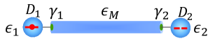
Figure 1: Schematic drawing for the setup of a Majorana quantum wire coupled to two quantum dots. The single electron is assumed initially in the left dot and the subsequent evolution is expected to display a ‘teleportation’ type quantum oscillations between the remotely distant dots.

II Revisit the issue of Majorana teleportation

II.1 Low-Energy Effective Model and
Number-State Treatment

About the issue of ‘teleportation’, let us consider first the simplest ‘quantum dot–Majorana wire–quantum dot’ setup (see Fig. 1), following Refs. Lee08 ; Fu10 , to analyze the quantum transfer and oscillation of an electron through a quantum wire which accommodates a pair of Majorana bound states (MBSs). The setup of Fig. 1 can be described by the following effective low-energy Hamiltonian

$$H=i\frac{\epsilon_{M}}{2}\gamma_{1}\gamma_{2}+\sum_{j=1,2}\big{[}\epsilon_{j}d^{\dagger}_{j}d_{j}+\lambda_{j}(d^{\dagger}_{j}-d_{j})\gamma_{j}\big{]}\,.$$ (1)

Here $\gamma_{1}$ and $\gamma_{2}$ are the Majorana operators for the two MBSs at the ends of the quantum wire. The two MBSs interact with each other by an energy $\epsilon_{M}$. $d_{1}(d^{\dagger}_{1})$ and $d_{2}(d^{\dagger}_{2})$ are the annihilation (creation) operators of the two single-level quantum dots, while $\lambda_{1}$ and $\lambda_{2}$ are their coupling amplitudes to the MBSs. The Majorana operators are related to the regular fermion through the transformation of $\gamma_{1}=i(f-f^{\dagger})$ and $\gamma_{2}=f+f^{\dagger}$. After an additional local gauge transformation, $d_{1}\to id_{1}$, we reexpress Eq. (1) as

$$H = \epsilon_{M}(f^{\dagger}f-\frac{1}{2})+\sum_{j=1,2}[\epsilon_{j}d^{\dagger}_{j}d_{j}+\lambda_{j}(d^{\dagger}_{j}f+f^{\dagger}d_{j})]$$ (2)

$$-\lambda_{1}(d^{\dagger}_{1}f^{\dagger}+fd_{1})+\lambda_{2}(d^{\dagger}_{2}f^{\dagger}+fd_{2})\,.$$

It should be noticed that the tunneling terms in this Hamiltonian only conserve charge modulo $2e$. This reflects the fact that a pair of electrons can be extracted from the superconductor condensate and can be absorbed by the condensate vice versa.

Let us consider the transfer of an electron between the two quantum dots, which is assumed initially in the left quantum dot. In particular, we consider the weak interaction limit $\epsilon_{M}\to 0$, in order to reveal more drastically the teleportation behavior. For simplicity, we assume $\lambda_{1}=\lambda_{2}=\lambda$ and $\epsilon_{1}=\epsilon_{2}=0$. Using the regular fermion number-state representation, i.e., ${\left|n_{1},n_{f},n_{2}\right\rangle}$, where $n_{1(2)}$ and $n_{f}$ denote respectively the electron numbers (“0” or “1”) in the left (right) dot and the central MZMs, we have eight basis states: ${\left|100\right\rangle},{\left|010\right\rangle},{\left|001\right\rangle},{\left|111\right\rangle}$ with odd parity (electron numbers); and ${\left|110\right\rangle},{\left|101\right\rangle},{\left|011\right\rangle},{\left|000\right\rangle}$ with even parity. Associated with the specific initial condition, we only have the odd-parity states involved in the state evolution.

Starting with the initial state $|100\rangle$, the state evolution within the odd-parity subspace can be carried out straightforwardly Lee08 . Specifically, we are interested in the probability of electron appearing in the right dot, which has two components Lee08

$$P^{(1)}_{2}(\tau) = |\langle 001|e^{-iH\tau}{\left|100\right\rangle}|^{2}=\sin^{4}(\lambda\tau)\,,$$

$$P^{(2)}_{2}(\tau) = |\langle 111|e^{-iH\tau}{\left|100\right\rangle}|^{2}=\frac{1}{4}\sin^{2}(2\lambda\tau)\,.$$ (3)

Of great interest is the result of $P^{(1)}_{2}(\tau)$, which implies that, even in the limit of $\epsilon_{M}\to 0$ (very long quantum wire), the electron in the left dot can transmit through the quantum wire and reappear in the right dot on a finite (short) timescale. This is the remarkable ‘teleportation’ phenomenon discussed in Refs. Sem06ab ; Lee08 ; Fu10 which, surprisingly, holds a superluminal feature.

However, the result of $P^{(2)}_{2}(\tau)$ is associated with the Andreev process, i.e., splitting of a Cooper pair from the condensate of the superconductor. To be more specific, let us consider the initial state $|100\rangle$. The state $|111\rangle$ can be generated from $|100\rangle$ by the local Andreev process at the right-hand-side, which is described by the effective tunneling term $d^{\dagger}_{2}f^{\dagger}$ in Eq. (2). Obviously, this is not the event of teleportation of interest, since the electron appearing in the right dot ($D_{2}$) is not the one initially prepared in the left dot ($D_{1}$). In order to single out the teleportation channel from the Andreev process, it would be highly desirable if we can suppress the terms ($\lambda_{j}d^{\dagger}_{j}f^{\dagger}+{\rm h.c.}$) in Eq. (2).

Indeed, it was proposed in Ref. Fu10 that a nanowire is in proximity contact with a mesoscopic floating superconductor with strong charging energy $E_{C}$. Under such assumptions, it was derived by an elegant and precise treatment that the tunnel coupling is truncated to the following Hamiltonian of tunneling through a single resonant level Fu10

$$H = \epsilon_{M}(f^{\dagger}f-\frac{1}{2})+\sum_{j=1,2}\big{[}\epsilon_{j}d^{\dagger}_{j}d_{j}+\lambda_{j}(d^{\dagger}_{j}f+f^{\dagger}d_{j})\big{]}\,.$$

Comparing this result with the tunneling Hamiltonian in Eq. (2), we find that the Andreev process terms have been ruled out and that the only survived charge transfer channel is the real transmission through the nonlocal Majorana states. This is the true teleportation channel of our interest.

As an additional remark, it should be noted that the suppression of the Andreev process terms does not mean the superconducting pairing term destroyed. Actually, the superconducting pairing term has been taken into account when diagonalizing the superconductor Hamiltonian, which is responsible to the formation of both the ground state condensate and the quasiparticle states (including the Majorana $f$ quasiparticle). The tunnel coupling Hamiltonians in both Eqs. (2) and (II.1) are an effective low-energy description.

After suppressing the Andreev process, the transfer dynamics only involves states ${\left|100\right\rangle}$, ${\left|010\right\rangle}$, and ${\left|001\right\rangle}$. The time dependent state can be therefore expressed as $|\Psi(\tau)\rangle=a(\tau){\left|100\right\rangle}+b(\tau){\left|010\right\rangle}+c(\tau){\left|001\right\rangle}$. Also, we consider the simplest case by assuming $\epsilon_{M}=\epsilon_{1}=\epsilon_{2}=0$ and $\lambda_{1}=\lambda_{2}=\lambda$. Solving the Schrödinger equation based on the Hamiltonian Eq. (II.1) yields

$$a(\tau) = \frac{1}{2}\left[1+\cos(\sqrt{2}\lambda\tau)\right]\,,$$

$$b(\tau) = -\frac{i}{\sqrt{2}}\sin(\sqrt{2}\lambda\tau)\,,$$

$$c(\tau) = \frac{1}{2}\left[-1+\cos(\sqrt{2}\lambda\tau)\right]\,.$$ (5)

This solution was obtained with the initial condition $|\Psi(0)\rangle={\left|100\right\rangle}$. Therefore, the occupation probability of the right dot, $P_{2}(\tau)=|c(\tau)|^{2}=\sin^{4}(\lambda\tau/\sqrt{2})$, reveals a real teleportation feature as discussed above based on $P_{2}^{(1)}(\tau)$ in Eq. (II.1). In Fig. 2(a), using the above analytic solution, we plot the occupation probabilities of the two dots (by the black and red lines). The displayed simple quantum oscillations are indeed remarkable, viewing that the two dots are coupled through a very long quantum wire.

II.2 Bogoliubov-de Gennes Equation Based Simulation

We now turn to a lattice-model-based simulation for the above transfer dynamics using the BdG equation and the well known Kitaev model for the topological quantum wire Kita01

$$H_{W} = \sum_{j}\left[-\mu c^{\dagger}_{j}c_{j}-\frac{t}{2}(c^{\dagger}_{j}c_{j+1}+{\rm h.c.})\right]$$ (6)

$$+\frac{\Delta}{2}\sum_{j}(c_{j}c_{j+1}+{\rm h.c.})\,.$$

In this spinless $p$-wave superconductor model, $\mu$ is the chemical potential, $\Delta$ is the superconducting order parameter, and $t$ is the hopping energy between the nearest neighbor sites with $c^{\dagger}_{j}$ ($c_{j}$) the associated electron creation (annihilation) operators. The specific choice of $\frac{t}{2}$ and $\frac{\Delta}{2}$ is for a convenience such that the energy gap parameter of the quasiparticle excitations is $\Delta$ (rather than $2\Delta$). The total Hamiltonian of the setup shown in Fig. 1 reads $H=H_{W}+H_{D}+H^{\prime}$, with $H_{D}=\sum_{j=1,2}\epsilon_{j}d^{\dagger}_{j}d_{j}$ and the coupling between the dots and the quantum wire given by

$$H^{\prime}=(t_{L}d_{1}c^{\dagger}_{1}+t_{R}d_{2}c^{\dagger}_{N})+{\rm h.c.}\,,$$ (7)

with $t_{L}$ and $t_{R}$ the coupling energies.

In order to introduce the representation of electron and hole states, we use the Nambu spinor $\hat{\Psi}=(c_{1},\cdots,c_{N},c^{\dagger}_{1},\cdots,c^{\dagger}_{N})^{T}$ and rewrite the Hamiltonian of the quantum wire as $H_{W}=\frac{1}{2}\hat{\Psi}^{\dagger}\tilde{H}_{W}\hat{\Psi}$, which yields thus the BdG Hamiltonian matrix

$$\tilde{H}_{W}=\left(\begin{array}[]{cc}T&\Omega\\ -\Omega&-T\end{array}\right)\,,$$ (10)

where the block elements are given by

$$T=\left(\begin{array}[]{ccccc}-\mu&-t/2&0&\cdots&\cdots\\ -t/2&-\mu&-t/2&0&\cdots\\ 0&-t/2&-\mu&-t/2&\cdots\\ \cdot&\cdot&\cdot&\cdot&\cdot\\ \cdot&\cdot&\cdot&\cdot&\cdot\end{array}\right)\,,$$ (16)

and

$$\Omega=\frac{1}{2}\left(\begin{array}[]{ccccc}0&\Delta&0&\cdots&\cdots\\ -\Delta&0&\Delta&0&\cdots\\ 0&-\Delta&0&\Delta&\cdots\\ \cdot&\cdot&\cdot&\cdot&\cdot\\ \cdot&\cdot&\cdot&\cdot&\cdot\end{array}\right)\,.$$ (22)

More physically, the above BdG Hamiltonian matrix can be understood as being constructed under the single-particle basis $\{|e_{1}\rangle,\cdots,|e_{N}\rangle;~{}|h_{1}\rangle,\cdots,|h_{N}\rangle\}$, where $|e_{j}\rangle$ and $|h_{j}\rangle$ describe, respectively, the electron and hole states on the $j$th site.

Further, let us consider the entire ‘Dot-Wire-Dot’ system. Using the joint electron and hole basis, the complete states of the quantm dots should include both $|D_{j}\rangle$ and $|H_{j}\rangle$, with $j=1,2$ labeling the quantum dots while ‘$D$’ and ‘$H$’ describing the electron and hole states, respectively. Accordingly, the Hamiltonian should include couplings of $|D_{1}\rangle$ with $|e_{1}\rangle$ and $|D_{2}\rangle$ with $|e_{N}\rangle$ for electrons, and $|H_{1}\rangle$ with $|h_{1}\rangle$ and $|H_{2}\rangle$ with $|h_{N}\rangle$ for holes. It is well known that the hole couplings are employed to describe the Andreev process. For instance, in the simplified description of the low-energy excitations, the transition $|1,0,0\rangle\Rightarrow|1,1,1\rangle$ corresponds to annihilating the hole state $|H_{2}\rangle$ (owing to the transfer of $|H_{2}\rangle$ to $|h_{N}\rangle$), and at the same time exciting the ‘$f$’ quasi-particle of the MZMs (via the $|h_{N}\rangle$ excitation). Similarly, the transition $|1,1,1\rangle\Rightarrow|0,0,1\rangle$ is mediated by the hole transfer from $|h_{1}\rangle$ of the wire to $|H_{1}\rangle$ of the left dot.

To make a close comparison between the effective low-energy model result and the Kitaev lattice model based simulation, we restrict our analysis to the transfer dynamics associated with the truncated ‘teleportation’ Hamiltonian, Eq. (II.1), where only the teleportation channel is left while the Andreev process is suppressed. Then, in the absence of hole couplings between the dots and the quantum wire, the coupling Hamiltonian reads

$$H^{\prime}=(t_{L}|e_{1}\rangle\langle D_{1}|+t_{R}|e_{N}\rangle\langle D_{2}|)+{\rm h.c.}\,.$$ (23)

Again, let us consider the evolution starting with $|\Psi(0)\rangle=|D_{1}\rangle$, i.e., initially the electron in the left dot. The transfer dynamics is described by

$$|\Psi(\tau)\rangle=\alpha_{1}(\tau)|D_{1}\rangle+\alpha_{2}(\tau)|D_{2}\rangle$$

$$~{}~{}~{}~{}~{}~{}+\sum^{N}_{j=1}[u_{j}(\tau)|e_{j}\rangle+v_{j}(\tau)|h_{j}\rangle]\,,$$ (24)

where the superposition coefficients can be solved from the time-dependent Schrödinger equation, $i\hbar\frac{\partial}{\partial\tau}|\Psi(\tau)\rangle=H|\Psi(\tau)\rangle$, by casting the Hamiltonian into the BdG-type matrix form, using the joint electron and hole basis.

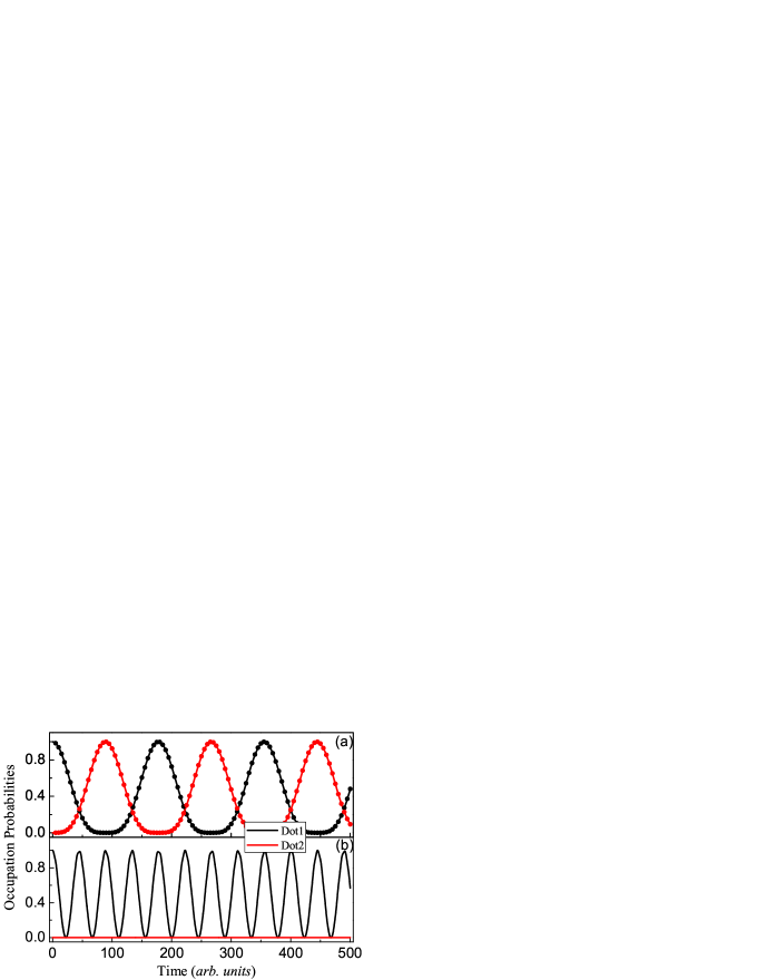
Figure 2: Quantum oscillations of an electron between two remote quantum dots, mediated by the nonlocal MZMs. (a) Plots of the analytic solution Eq. (II.1) (black and red lines, based on the number-states treatment of the low-energy effective model), compared with the results from the lattice model based simulation using the tunneling Hamiltonian Eq. (25) (black and red dots). Through the whole work we adopt an arbitrary system of units by setting the hopping energy in the Kitaev lattice model $t=1$. Other parameters in the lattice model: $\epsilon_{1}=\epsilon_{2}=0$, $t_{L}=t_{R}=0.05$, $\mu=0$ and $\Delta=1.0$. The corresponding parameters of the reduced low-energy effective model: $\epsilon_{M}=0$ and $\lambda_{1}=\lambda_{2}=\lambda=0.025$. (b) Results based on the Kitaev lattice model and using the tunneling Hamiltonian Eq. (23), which involves both the positive and negative energy eigenstates in the dynamics. Parameters are the same as in (a).

In Fig. 2(b) we show the results from numerically solving Eq. (II.2). To compare with the results displayed in Fig. 2(a), we plot the probabilities $P_{1}(\tau)=|\alpha_{1}(\tau)|^{2}$ and $P_{2}(\tau)=|\alpha_{2}(\tau)|^{2}$ by the black and red lines, respectively. Most surprisingly, in Fig. 2(b), we find no occupation of the right dot with the increase of time, which simply means no charge transfer mediated by the MZMs. We only find quantum oscillations between the left dot and the quantum wire, but with a period differing from that in Fig. 2(a), despite that in both plots we have used identical coupling strengths. We may identify the reasons for both results as follows.

By diagonalizing the BdG Hamiltonian $\tilde{H}_{W}$ of the quantum wire, one obtains two sets of eigenstates, say, $|E_{n}\rangle$ and $|-E_{n}\rangle$ with $n=1,2,\cdots,N$, corresponding to the positive and negative eigen-energies. In particular, in the topological regime, the lowest energy states $|E_{1}\rangle$ and $|-E_{1}\rangle$ are sub-gap states with $E_{1}\to 0$ and the wavefunctions distribute at the ends of the quantum wire. The MBSs at the ends of the wire are obtained from, respectively, $|\gamma_{1}\rangle=(|E_{1}\rangle+|-E_{1}\rangle)/2$ and $|\gamma_{2}\rangle=(|E_{1}\rangle-|-E_{1}\rangle)/2i$. From the tunnel Hamiltonian Eq. (23), the charge transfer $|D_{1}\rangle\to|e_{1}\rangle$ will generate a quantum superposition of $|E_{1}\rangle$ and $|-E_{1}\rangle$ in the quantum wire, especially with equal weights as $E_{1}\to 0$. Owing to the requirement of energy conservation, the higher eigen-energy states will not be excited (populated) after a timescale longer than $\hbar/t_{L}$. As a consequence of this superposition of $|E_{1}\rangle$ and $|-E_{1}\rangle$, the electron and hole excitations are largely located at the left side of the wire, leading thus to no charge transfer to the right side of the wire and to the right side quantum dot.

The simultaneous coupling of $|D_{1}\rangle$ to the zero-energy states $|E_{1}\rangle$ and $|-E_{1}\rangle$ of the quantum wire is also the reason for the different periods of oscillations in Fig. 2(b) and (a).

We understand then that the main difference of the coupling Hamiltonian Eq. (23) from the ‘number’-states treatment using the low-energy effective model is the redundant coupling of the dot electron to the negative-energy eigenstates of the superconducting quantum wire. Indeed, the negative-energy eigenstates are the dual counterparts of the Bogoliubov quasi-particles (the positive-energy eigenstates). Before diagonalizing the Hamiltonian of the superconductor, introducing holes (with negative energies) is unavoidable, in order to ‘mix’ the electron and hole components to form the Bogoliubov quasi-particles (physically, owing to the many body electron-electron scattering and the existence of the superconducting condensate). However, after the diagonalization, the negative-energy eigenstates are redundant. A negative-energy eigenstate simply means the result of removing an existing quasi-particle (which has positive energy). Moreover, the corresponding Bogoliubov ‘creation’ operators of the negative-energy eigenstates will, importantly, annihilate the ground state of the superconductor. In other words, the negative-energy eigenstates cannot be created from the ground state of the superconductor. Therefore, if we explicitly introduce the creation of Bogoliubov positive-energy quasiparticles (from the ground state) and annihilation of the existing ones, the negative-energy eigenstates are redundant, which should not appear in the tunnel coupling Hamiltonian.

For the specific setup under consideration, the tunnel coupling Hamiltonian should thus be modified as

$$H^{\prime}=(t_{L}|\tilde{e}_{1}\rangle\langle D_{1}|+t_{R}|\tilde{e}_{N}\rangle\langle D_{2}|)+{\rm h.c.}\,,$$ (25)

where the two projected states are defined through

$$|\tilde{e}_{1}\rangle = \hat{P}|e_{1}\rangle\,,$$

$$|\tilde{e}_{N}\rangle = \hat{P}|e_{N}\rangle\,,$$ (26)

while the projection operator is defined by

$$\hat{P}=\sum^{N}_{E_{n}>0,~{}n=1}|E_{n}\rangle\langle E_{n}|\,.$$ (27)

Very importantly, the above tunneling Hamiltonian properly accounts for the creation and annihilation of the Bogoliubov quasiparticles (with positive energies), which are the real existence in superconductors. Here, owing to the suppression of the Andreev process, the hole states of the quantum dots do not appear in the tunnel coupling to the Bogoliubov quasiparticles. Otherwise, in the presence of Andreev process, as we will see later, the hole states of the transport leads will participate in the coupling to the Bogoliubov quasiparticles.

Based on the tunnel Hamiltonian Eq. (25), we re-simulate the electron transfer dynamics and obtain results shown in Fig. 2(a) by the symbols of black and red dots. In contrast to what we observed in Fig. 2(b), here the desired quantum oscillations are recovered in precise agreement with the number-state treatment based on the low-energy effective model. We should mention that this full agreement is achieved in the regime of weak coupling between the dots and the quantum wire, which guarantees the dominant coupling of the quantum dots being to the MZMs, but not to the Bogoliubov quasiparticle states above the superconducting gap. If we consider a strong coupling regime, occupation of the quasiparticle states above the gap will result in some irregularities instead of the ideal quantum oscillations.

II.3 On the Teleportation Issue

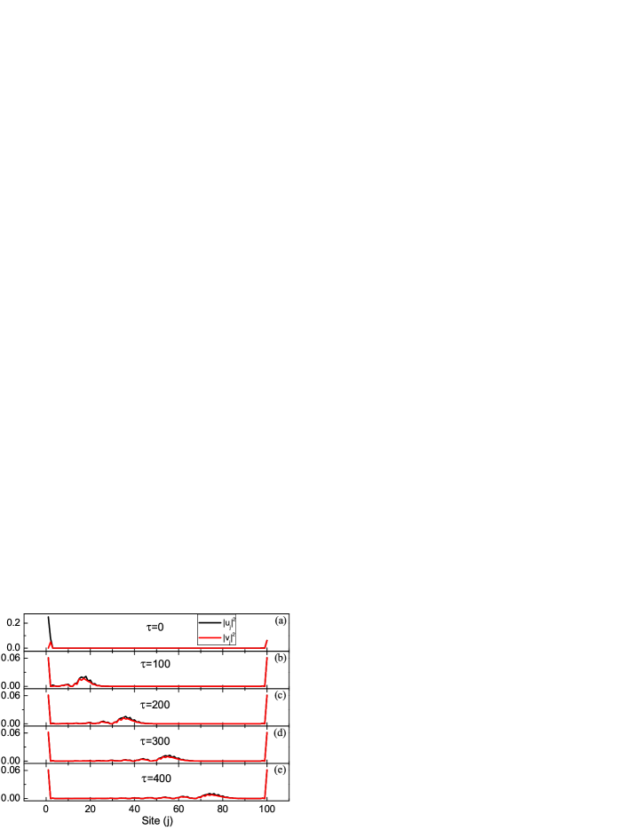
Figure 3: Wavepacket propagation of the electron-hole excitations based on simulation of the isolated Kitaev’s lattice wire. We adopt an arbitrary system of units by setting the hopping energy $t=1$ (and $\hbar=1$), and assume the other parameters $\mu=0$ and $\Delta=0.8$. (a) Initial distribution of the electron-hole excitations after projecting the lattice state $|e_{1}\rangle$ onto the Hilbert space of the Bogoliubov quasiparticle states, which corresponds to the action of $c_{1}^{\dagger}$ on the superconductor ground state $|G\rangle$. (b)-(e) Propagation of the electron-hole excitations along the lattice wire with the increase of time ($\tau$).

Taking the lattice model, let us first simulate the ‘microscopic’ dynamics of the electron-hole excitations in the quantum wire. Without loss of the main physics, as a simpler and clearer illustration, we may consider an isolated quantum wire with an initial excitation of $|e_{1}\rangle$. This corresponds to the electron in the left dot ($D_{1}$) entering the wire via the first site, i.e., $|\tilde{e}_{1}\rangle=c_{1}^{\dagger}|G\rangle=\hat{P}|e_{1}\rangle$, where $|G\rangle$ is the ground state of the superconductor wire. Note that, owing to the property (requirement) of the ground state, the real physical state is $|\tilde{e}_{1}\rangle$ but not $|e_{1}\rangle$.

Specifically, let us assume $\mu=0$ and $\Delta=0.8$ (note that we always set $t=1$ through the whole work). We find that, from the initial ‘lattice state’ $|e_{1}\rangle$, the projection probability of getting the Majorana state $|E_{1}\rangle$ is, $p_{1}=|\langle E_{1}|e_{1}\rangle|^{2}\simeq 0.247$. In the ideal case of $\Delta=t$, this probability is $p_{1}=0.25$. In Fig. 3(a), we show the initial electron-hole excitations from the (unnormalized) projected state $|\tilde{e}_{1}\rangle=\hat{P}|e_{1}\rangle$. The result displayed by the red curve in Fig. 3(a) is the distribution of the hole components on the lattice sites, which largely characterizes the distribution of the electron-hole excitations in the Majorana state $|E_{1}\rangle$, by noting that the weights of the electron and hole components are equal i.e., $|u_{j}|^{2}=|v_{j}|^{2}$ on every lattice site, for $E_{1}\simeq 0$. However, on the left side, owing to the quantum superposition with the high energy states and thus the quantum interference, the hole distribution has some distortion compared to the right side, where this same effect is negligibly weak. The black curve in Fig. 3(a) more heavily involves the electron-component contribution of the high energy states above the gap, with their superposition resulting in the localized distribution in space. In Fig. 3(b)-(e), we show the wavepacket propagation of the electron-hole excitations. It should be noted that the propagation is largely from the electron-hole excitations of the high energy states. The two-side edge distributions associated with zero-energy Majorana mode are almost unaffected from the evolution.

The picture revealed in Fig. 3 indicates that the charge transfer mediated by the Majorana state is not via the wavepacket propagation of the electron-hole excitations along the wire. Once the external electron enters the wire, the two-side edge excitations associated with the MZMs are generated instantaneously, thus holding the ‘teleportation’ ability to mediate charge transfer. We may argue this extremely puzzling issue with a few remarks in order as follows.

(i) We notice that in Ref. Lee08 , in order to rule out the difficulty of arriving to a ‘superluminal’ conclusion, it was argued that since a classical exchange of information (the result of the coincident measurements) is necessary, there is no superluminal transfer of information in the observation of the teleportation effect. However, as pointed out in Ref. Li14b , in principle one can confirm the ‘teleportation event’ in a later stage from the coincident measurement data of two remote detectors. Obviously, this confirmation for the existing objective event does not need any communication of classical information.

(ii) Unlike the argument in Ref. Lee08 , we may provide an alternative understanding. Since the Majorana state is a quasiparticle excitation in the presence of many other electrons (condensate of the superconductor ground state), we cannot conclude that the electron appeared in the right quantum dot is the one initially in the left dot. Indeed, consider the action of $c_{1}^{\dagger}$ on the superconductor ground state $|G\rangle$. viewing that $|G\rangle$ is a condensate of many electrons (superposition of occupied and unoccupied electron pairs), the action of $c_{1}^{\dagger}$ would induce a ‘reformation’ of the whole correlated many electron condensate. From the ‘re-organized’ condensate, the quasiparticle excitation can be separated with respect to the ground state. In particular, the Majorana state among the quasipaiticle excitations holds the nonlocal nature, as a superposition of the electron-hole excitations at the two ends of the quantum wire.

Obviously, the electron-hole components at the right side are not from the left side through any quantum transfer process. The new particle is formed as a result of ‘re-organization’ of the many-particle condensate. This re-organization process, which thus allows us to extract electron from the right side, may resemble in some sense the current formation in a conducting wire under electric field, where the current forming at a remote place is not from the electrons of the initial place we performed electric disturbance. The speed of current formation in the conducting wire is not superluminal. Similarly, the ‘reorganization’ of the many electron condensate mentioned above cannot be superluminal. Therefore, the ‘superluminal’ feature of Majorana teleportation is a result that the ‘re-organization’ process of the many electron condensate did not enter a dynamical description.

(iii) The action of the local operator of $c_{1}^{\dagger}$ on the ground state, which causes the nonlocal excitation of the Majorana state, can be also understood from the perspective of quantum measurement. More specifically, in terms of the POVM (positive-operator-value-measure) formalism, let us consider $\tilde{\rho}=M\rho M^{\dagger}/||\bullet||$, with the Kraus measurement operator $M=c_{1}^{\dagger}$, the density matrix of the ground state $\rho=|G\rangle\langle G|$ and $||\bullet||$ denoting the normalization factor. We know that $c_{1}^{\dagger}$ can be decomposed into a superposition of the Bogoliubov operators, both the creation and annihilation operators. However, the action of the annihilation operators on the ground state would vanish the result. The state survived from this action is a superposition of the quasiparticle states generated by the creation operators. Among them, the particular Majorana state is highly nonlocal. Actually, the ‘measurement’ process described by the POVM projection should correspond to the ‘re-organization’ of the many electron condensate.

To summarize, the Majorana-nonlocality-induced teleportation looks like a superluminal phenomenon, but in reality it cannot be, if we take into account the re-organization process of the many electron condensate and/or the measurement process discussed above.

III Transport through Majorana quantum wires

III.1 Preliminary Consideration

As a more realistic configuration, let us consider to connect the quantum wire with two transport leads, instead of the quantum dots. The transport leads can be described by the interaction-free Hamiltonian

$$H_{\rm leads}=\sum_{l}\epsilon_{l}a^{\dagger}_{l}a_{l}+\sum_{r}\epsilon_{r}b^{\dagger}_{r}b_{r}\,,$$ (28)

and the coupling of the quantum wire to the leads is described by the tunnel Hamiltonian

$$H^{\prime}=\left(\sum_{l}t_{l}c^{\dagger}_{1}a_{l}+\sum_{r}t_{r}c^{\dagger}_{N}b_{r}\right)+{\rm h.c.}\,.$$ (29)

To display the Andreev process in a transparent manner, let us introduce the electron and hole basis $\{|e_{j}\rangle,|h_{j}\rangle~{}|~{}j=1,2,\cdots,N\}$ for the Kitaev quantum wire, and similarly $\{|e_{l}\rangle,|h_{l}\rangle\}$ and $\{|e_{r}\rangle,|h_{r}\rangle\}$ for the left and right leads. Using these basis states, the tunnel Hamiltonian can be rewritten as

$$H^{\prime}=\left[\sum_{l}t_{l}(|e_{1}\rangle\langle e_{l}|-|h_{1}\rangle\langle h_{l}|)\right.$$

$$~{}~{}~{}+\left.\sum_{r}t_{r}(|e_{N}\rangle\langle e_{r}|-|h_{N}\rangle\langle h_{r}|)\right]+{\rm h.c.}\,.$$ (30)

In particular, the tunnel coupling between the hole states in this form is explicitly used to describe the Andreev process. However, based on the lesson learned in the ‘Dot-Wire-Dot’ setup, we propose to modify the tunnel Hamiltonian as

$$H^{\prime}=\left[\sum_{l}t_{l}(|\tilde{e}_{1}\rangle\langle e_{l}|-|\tilde{h}_{1}\rangle\langle h_{l}|)\right.$$

$$~{}~{}~{}+\left.\sum_{r}t_{r}(|\tilde{e}_{N}\rangle\langle e_{r}|-|\tilde{h}_{N}\rangle\langle h_{r}|)\right]+{\rm h.c.}\,,$$ (31)

where the lattice edge site states (for both electrons and holes) are projected onto the subspace of the Bogoliubov quasiparticle states, through the projector $\hat{P}$ introduced previously by Eq. (27).

III.2 Single Particle Wavefunction Approach

For mesoscopic quantum transports, there exist well known approaches such as the nonequilibrium Green’s function (nGF) method Jau96 ; Datt95 and the S-matrix quantum scattering theory Datt95 ; Gla02 which are particularly suitable, in the absence of many-body interactions, to study transport through a large system modeled by the tight-binding lattice model and with superconductors involved (either as the leads or a central device). Another less-developed method, say, the single particle wavefunction (SPWF) approach SG91 ; Li09 ; Li12b ; SG16 , is an alternative but attractive choice. This method, directly based on the time-dependent Schrödinger equation, was developed in the context of transport through small systems such as quantum dots and has been applied skillfully to study some interesting problems SG16 . Below we extend it to study quantum transports through large lattice systems, especially in the presence of superconductors which may result in rich physics such as Andreev reflections and phenomena related to the MZMs. Importantly, this method can be regarded as an extension of the S-matrix scattering theory, i.e., from stationary to transient versions. For instance, this method should be very useful to study the possible transport probe of non-adiabatic transitions during Majorana braiding in the context of topological quantum computations.

The basic idea of the SPWF method is keeping track of the quantum evolution of an electron initially in the source lead, based on the time-dependent Schrödinger equation, and computing various transition rates such as the transmission rate to the drain lead, or Andreev-reflection rate back to the source lead as a hole. For the problem under study, we denote the initial state as $|\Psi(0)\rangle=|e_{\bar{l}}\rangle$. The subsequent evolution will result in a superposition of all basis states of the leads and the central device, expressed as

$$|\Psi\rangle=|\Psi_{w}\rangle+|\Psi_{\rm leads}\rangle$$

$$=\sum^{N}_{j=1}(u_{j}|e_{j}\rangle+v_{j}|h_{j}\rangle)+\sum_{l}(\alpha_{l}|e_{l}\rangle+\tilde{\alpha}_{l}|h_{l}\rangle)$$

$$~{}~{}+\sum_{r}(\beta_{r}|e_{r}\rangle+\tilde{\beta}_{r}|h_{r}\rangle)\,.$$ (32)

Based on the time dependent Schrödinger equation, $i|\dot{\Psi}\rangle=H|\Psi\rangle$, we have

$$i\,\dot{u}_{j} = (\bullet)+\sum_{l}t_{l}\alpha_{l}\langle e_{j}|\tilde{e}_{1}\rangle+\sum_{l}(-t_{l})\tilde{\alpha}_{l}\langle e_{j}|\tilde{h}_{1}\rangle$$

$$~{}~{}+\sum_{r}t_{r}\beta_{r}\langle e_{j}|\tilde{e}_{N}\rangle+\sum_{r}(-t_{r})\tilde{\beta}_{r}\langle e_{j}|\tilde{h}_{N}\rangle$$

$$i\,\dot{v}_{j} = (\bullet)+\sum_{l}t_{l}\alpha_{l}\langle h_{j}|\tilde{e}_{1}\rangle+\sum_{l}(-t_{l})\tilde{\alpha}_{l}\langle h_{j}|\tilde{h}_{1}\rangle$$

$$~{}~{}+\sum_{r}t_{r}\beta_{r}\langle h_{j}|\tilde{e}_{N}\rangle+\sum_{r}(-t_{r})\tilde{\beta}_{r}\langle h_{j}|\tilde{h}_{N}\rangle$$

$$i\,\dot{\alpha}_{l} = \epsilon_{l}\alpha_{l}+t^{*}_{l}\langle\tilde{e}_{1}|\Psi_{w}\rangle$$

$$i\,\dot{\tilde{\alpha}}_{l} = -\epsilon_{l}\tilde{\alpha}_{l}-t^{*}_{l}\langle\tilde{h}_{1}|\Psi_{w}\rangle$$

$$i\,\dot{\beta}_{r} = \epsilon_{r}\beta_{r}+t^{*}_{r}\langle\tilde{e}_{N}|\Psi_{w}\rangle$$

$$i\,\dot{\tilde{\beta}}_{r} = -\epsilon_{r}\tilde{\beta}_{r}-t^{*}_{r}\langle\tilde{h}_{N}|\Psi_{w}\rangle$$ (33)

For the sake of brevity, in the first two equations, we have used the symbol $(\bullet)$ to denote the terms for the central system (in the absence of coupling to leads). Performing the Laplace and inverse-Laplace transformations, after some algebras, we obtain

$$i\,\dot{u}_{j} = (\bullet)-i\frac{\Gamma_{L}}{2}\,\left[\langle e_{j}|\tilde{e}_{1}\rangle\langle\tilde{e}_{1}|\Psi_{w}\rangle+\langle e_{j}|\tilde{h}_{1}\rangle\langle\tilde{h}_{1}|\Psi_{w}\rangle\right]$$

$$-i\frac{\Gamma_{R}}{2}\,\left[\langle e_{j}|\tilde{e}_{N}\rangle\langle\tilde{e}_{N}|\Psi_{w}\rangle+\langle e_{j}|\tilde{h}_{N}\rangle\langle\tilde{h}_{N}|\Psi_{w}\rangle\right]$$

$$+t_{L}e^{-iE_{\rm in}t}\langle e_{j}|\tilde{e}_{1}\rangle$$

$$i\,\dot{v}_{j} = (\bullet)-i\frac{\Gamma_{L}}{2}\,\left[\langle h_{j}|\tilde{e}_{1}\rangle\langle\tilde{e}_{1}|\Psi_{w}\rangle+\langle h_{j}|\tilde{h}_{1}\rangle\langle\tilde{h}_{1}|\Psi_{w}\rangle\right]$$ (34)

$$-i\frac{\Gamma_{R}}{2}\,\left[\langle h_{j}|\tilde{e}_{N}\rangle\langle\tilde{e}_{N}|\Psi_{w}\rangle+\langle h_{j}|\tilde{h}_{N}\rangle\langle\tilde{h}_{N}|\Psi_{w}\rangle\right]$$

$$+t_{L}e^{-iE_{\rm in}t}\langle h_{j}|\tilde{e}_{1}\rangle$$

In a more compact form, the result can be reexpressed as

$$i\begin{bmatrix}\dot{u}_{1}\\ \dot{u}_{2}\\ \vdots\\ \dot{u}_{N}\\ \dot{v}_{1}\\ \dot{v}_{2}\\ \vdots\\ \dot{v}_{N}\end{bmatrix}=(\bullet)+\left(\hat{P}\Sigma\hat{P}\right)\begin{bmatrix}u_{1}\\ u_{2}\\ \vdots\\ u_{N}\\ v_{1}\\ v_{2}\\ \vdots\\ v_{N}\end{bmatrix}+t_{L}e^{-iE_{\rm in}t}\hat{P}\begin{bmatrix}1\\ 0\\ 0\\ 0\\ \vdots\\ 0\\ 0\\ 0\\ 0\end{bmatrix}$$ (35)

where we introduce the self-energy operator as

$$\Sigma=(-i\Gamma_{L}/2)\,(|e_{1}\rangle\langle e_{1}|+|h_{1}\rangle\langle h_{1}|)$$

$$~{}~{}+(-i\Gamma_{R}/2)\,(|e_{N}\rangle\langle e_{N}|+|h_{N}\rangle\langle h_{N}|)\,.$$ (36)

Eq. (35) describes the evolution dynamics of the electron-hole excitations, in the presence of tunnel-couplings to the transport leads which lead to the self-energy term, i.e., the second term on the right-hand-side (r.h.s) of Eq. (35) together with Eq. (III.2). The third term on the r.h.s of Eq. (35) is resulted from the tunnel-coupling which injects the initial electron into the quantum wire. For both of the two terms, only the real (positive-energy) Bogoliubov quasiparticle states participate in the tunneling process, as imposed by the projection operator. Again, we emphasize that the projection eliminates the redundancy (‘double-use’) of the negative-energy eigenstates to be involved in the tunneling process. Physically speaking, the negative-energy eigenstate simply means the consequence of annihilating an existing positive-energy quasiparticle via, for instance, the usual tunneling or the more dramatic Andreev process. These two processes, by using only the positive-energy eigenstates, have been already accounted for in the treatment of the tunnel couplings, i.e., in Eq. (III.1). However, we may notice that Eq. (35) does not exclude any possible presence of the negative-energy eigenstates during the inside electron-hole excitation dynamics in the quantum wire.

It is clear that, based on the time-dependent state $|\Psi_{w}(t)\rangle$ given by Eq. (35), one can straightforwardly compute the various current components by finding first the projected occupation probabilities of the terminal sites of the quantum wire (for both the electron and hole components), then multiplying the tunnel-coupling rates, which yields

$$i_{\rm LR} = e\Gamma_{R}\,|\langle e_{N}|\hat{P}|\Psi_{w}\rangle|^{2}\,,$$

$$i_{\rm A} = e\Gamma_{L}\,|\langle h_{1}|\hat{P}|\Psi_{w}\rangle|^{2}\,,$$

$$i_{\rm CA} = e\Gamma_{R}\,|\langle h_{N}|\hat{P}|\Psi_{w}\rangle|^{2}\,,$$ (37)

where $e$ is the electron charge. These are the single-incident-electron (initially in $|e_{\bar{l}}\rangle$) contributed current components associated with, respectively, the normal electron transmission from the left to right leads, the local Andreev reflection at the left side, and the cross Andreev reflection process.

III.3 Connection with Other Approaches

To express the results in a more general form, let us denote the incident channel by $\alpha$, the outgoing channel by $\beta$, and the associated current by $i_{\alpha\beta}$. The ‘total’ current associated with the $(\alpha,\beta)$ channels from the incident electrons within the unit energy interval around $E$ is simply given by $\rho_{\alpha}(E)i_{\alpha\beta}(E)$, with $\rho_{\alpha}(E)$ the density-of-states at the incident energy. In long time limit (stationary limit), comparing this result with the current derived from the nonequilibrium Green’s function (nGF) technique Jau96 ; Datt95 , we can establish the following connection between the two approaches

$$\rho_{\alpha}(E)\,i_{\alpha\beta}(E)=\frac{e}{h}\,{\cal T}_{\alpha\beta}(E)\,.$$ (38)

In this expression, $h$ is the Plank constant and ${\cal T}_{\alpha\beta}(E)$ is the transmission coefficient from the channel $\alpha$ to $\beta$ at the energy $E$, which can be used to compute the linear-response or differential conductance by means of the well-known Landauer-Büttiker formula as $G_{\alpha\beta}=(e^{2}/h){\cal T}_{\alpha\beta}$. In this context, we like to mention that for the two-electron Andreev reflections, the respective conductance is related to the hole-reflection coefficient as $G_{\rm A}=(2e^{2}/h){\cal T}_{\rm A}$. Within the nGF formalism, the transmission coefficient is given by Jau96 ; Datt95

$${\cal T}_{\alpha\beta}(E)={\rm Tr}(\Gamma_{\alpha}G^{r}\Gamma_{\beta}G^{a})\,,$$ (39)

where $G^{r(a)}$ is the retarded (advanced) Green’s function of the transport central system, which includes the self-energies from the transport leads. Notice that, even within the nGF formalism, this result is valid only for transport through noninteracting systems. Another connection is that this formula corresponds to the S-matrix scattering approach Flen19b ; Bee08 ; Law09 ; Gla02 after summing all the final states of the scattering probability under the restriction of energy conservation, and for all the initial states at the energy $E$.

Applying the formula Eq. (39) to transport through a superconductor, straightforwardly, we can obtain the coefficients of the electron transmission (from left to right leads), the local Andreev reflection (in the left lead), and the cross Andreev reflection, respectively, as Sun01 ; Sun09 ; Li14

$${\cal T}_{\rm LR}(E) = {\rm Tr}\left(\Gamma^{e}_{L}G^{r}_{ee}\Gamma^{e}_{R}G^{a}_{ee}\right)\,,$$

$${\cal T}_{\rm A}(E) = {\rm Tr}\left(\Gamma^{e}_{L}G^{r}_{eh}\Gamma^{h}_{L}G^{a}_{he}\right)\,,$$

$${\cal T}_{\rm CA}(E) = {\rm Tr}\left(\Gamma^{e}_{L}G^{r}_{eh}\Gamma^{h}_{R}G^{a}_{he}\right)\,.$$ (40)

Here we have added explicitly the superscripts ‘$e$’ (for electrons) and ‘$h$’ (for holes) to the tunnel-coupling rates $\Gamma_{L}$ and $\Gamma_{R}$. We have also expressed the Green’s functions in an explicit form of matrix sector in the Nambu representation between the electron/hole states.

The above results of Eqs. (38)-(III.3) establish a connection at steady-state transport limit between the SPWF and nGF approaches, based on the standard BdG treatment without projection onto the space of positive-energy Bogoliubov quasiparticle states. In order to account for the modified treatment with projection, as a long-time stationary limit of Eq. (III.2), we only need to modify the Green’s functions in Eq. (III.3) as $\widetilde{G}^{r(a)}=\hat{P}G^{r(a)}\hat{P}$, together with the modified self-energies $\widetilde{\Sigma}^{r(a)}=\hat{P}\Sigma^{r(a)}\hat{P}$, as similarly done in Eq. (35) with the result of Eq. (III.2).

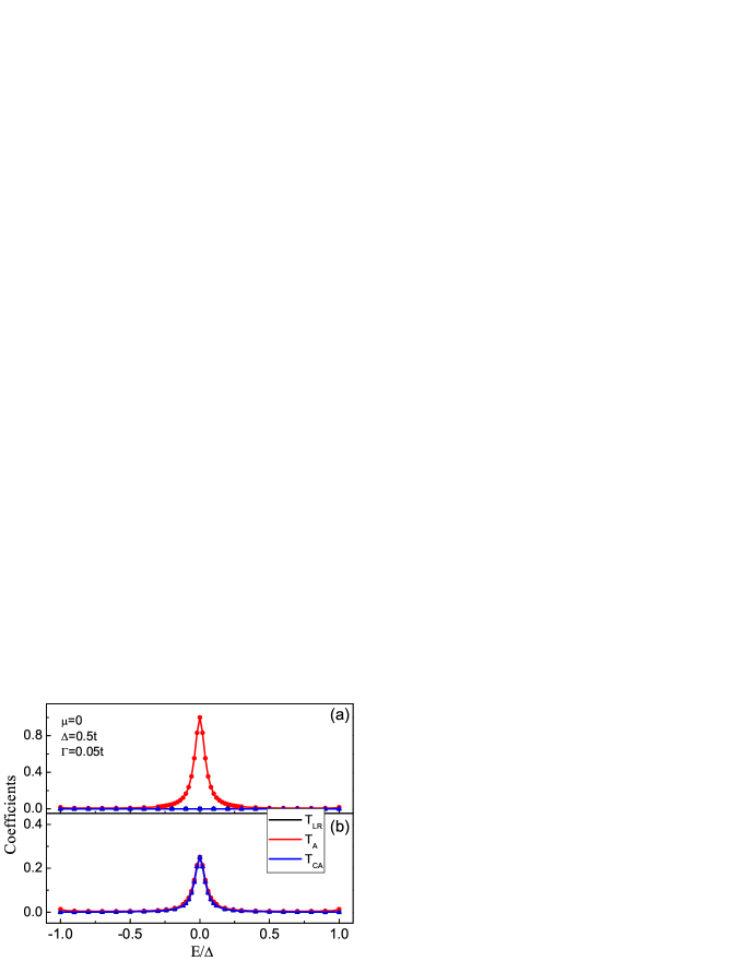
Figure 4: Kitaev’s lattice model based simulation for coefficients of transmission from the left to right leads (${\cal T}_{\rm LR}$), local Andreev reflection on the left side (${\cal T}_{\rm A}$), and cross Andreev reflection (${\cal T}_{\rm CA}$). Full agreement is achieved between the single-electron-wavefunction method (stationary limit) and the nonequilibrium Green’s function approach, as shown by the corresponding curves and dots. (a) Results based on simulation using the standard method of BdG equation with both the positive and negative energy eigenstates participating in the dynamics. Parameters: $\mu=0$, $\Delta=0.5$, $t=1.0$, and the tunnel coupling rates $\Gamma_{L}=\Gamma_{R}=\Gamma=0.05$. (b) Results from similar simulation as for (a), except keeping only the positive energy eigenstates by performing the projection as explained in the main text.

III.4 Results and Discussions

Indeed, the SPWF approach has the particular advantage to address time dependent transports. However, in this work we restrict our interest to stationary results of the transport.

Before displaying our numerical results, we first quote the analytical results based on the low-energy effective model and the S-matrix scattering approach Flen19b ; Bee08 ; Law09 ; Vu18 ; Gla02 . Using the results derived in Ref. Bee08 , we obtain the local Andreev reflection, the cross Andreev reflection, and the normal electron transmission coefficients (${\cal T}_{\rm A}$, ${\cal T}_{\rm CA}$, and ${\cal T}_{\rm LR}$), respectively, as

$${\cal T}_{\rm A}(E) = \Gamma^{2}_{L}(E^{2}+\Gamma^{2}_{R})/|Z|^{2}\,,$$

$${\cal T}_{\rm CA}(E) = {\cal T}_{\rm LR}(E)=\epsilon^{2}_{M}\Gamma_{L}\Gamma_{R}/|Z|^{2}\,,$$ (41)

where $Z=\epsilon^{2}_{M}-(E+i\Gamma_{L})(E+i\Gamma_{R})$. The same results can be obtained as well using Eq. (III.3), more straightforwardly.

In particular, under the limits of $\epsilon_{M}\to 0$ and $E\to 0$, we have ${\cal T}_{\rm A}\to 1$, being free from the coupling strength. We notice that in Ref. Law09 , this type of full Andreev-reflection (with unity coefficient) has been highlighted in terms of Majorana-fermion-induced resonant Andreev reflection. However, in Ref. Law09 , the local Andreev reflection is considered for the setup where only one bound state of the Majorana pair is coupled to the probe lead, while the other bound state is suspending (without coupling to any probe lead). This consideration corresponds to the setup of the standard two-probe tunneling spectroscopy experiment, which probes the local Andreev reflection taking place at the interface between a normal metal and grounded superconductor. Actually, the resonant Andreev reflection with ${\cal T}_{\rm A}\to 1$ will result in the quantized zero-bias differential conductance, $G=\frac{2e^{2}}{h}{\cal T}_{\rm A}\to 2e^{2}/h$. In this context, we may mention that for the local Andreev state, or, the so-called quasi-Majorana states Vu18 , the one more Majorana state coupled to the same lead will result in the conductance $G\to 4e^{2}/h$, under certain parameter conditions. The quantized conductance $2e^{2}/h$ has been extensively analyzed DS17 ; Vu18 ; DS01 ; Flen10 ; Flen16 and was regarded as an important signature of Majorana states Kou18a .

For the setup we consider here, both sides of the Majorana wire are coupled to probing leads. The fully ‘resonant’ Andreev reflection on the left side obtained also in this setup implies that the electron-hole excitation at the left side does not propagate to the other side, since no coupling effect of the other side is sensed in the probe of the local Andreev reflection. Based on Eq. (III.4), we observe another remarkable feature, say, under the limit $\epsilon_{M}\to 0$, ${\cal T}_{\rm CA}={\cal T}_{\rm LR}\to 0$. This type of vanishing cross Andreev reflection and normal electron transmission indicates also that the electron-hole excitations cannot propagate from one side to the other through the Majorana quantum wire.

Indeed, all the above features (from the low-energy effective model) are recovered in Fig. 4(a), by simulating the electron and hole dynamics based on the Kitaev lattice model using both the SPWF and nGF approaches, by setting $\hat{P}=1$ which corresponds to the conventional BdG treatment. However, the results of the vanishing cross Andreev reflection and normal electron transmission shown in Fig. 4(a) are not consistent with the electron transfer dynamics revealed from the simple ‘Dot-Wire-Dot’ system analyzed in Refs. Lee08 ; Fu10 , where the electron and hole excitations in the wire (described by the occupied state $|n_{f}=1\rangle$) do correlate the two quantum dots and can result in electron transfer and cross Andreev process between them.

In Fig. 4(b) we show the consistent results from new simulations, based on the same Kitaev lattice model and using both the SPWF and nGF approaches. In the new simulations, from the lesson learned earlier in the ‘Dot-Wire-Dot’ setup, we allow only coupling the electron and hole states of the leads to the positive-energy Bogoliubov quasiparticles in the wire, i.e., properly accounting for the projection of the wire states. Remarkably, we find essential differences, compared to Fig. 4(a). (i) The transmission and cross Andreev reflection coefficients are now nonzero in the limit $\epsilon_{M}\to 0$. The basic reason is that in the projected Hilbert subspace (after the action of the projector $\hat{P}$), no ‘cancellation’ of the electron-hole excitations occurs on the right side of the quantum wire, which yet would happen if including both the positive and negative zero-energy eigengenstates in the naive treatment. The results in Fig. 4(b) are now in agreement with the teleportation picture revealed in Refs. Lee08 ; Fu10 .   (ii) For the local Andreev reflection (on the left side), we find that the height of the reflection peak becomes 1/4, rather than 1 as observed in Fig. 4(a). We may understand this from the simplified low-energy effective model of the single MZMs coupled to two probe leads. Applying Eq. (III.3), we have

$${\cal T}_{A}(E)=\Gamma^{2}_{L}/|E-\epsilon_{M}-i(\Gamma_{L}+\Gamma_{R})|^{2}\,.$$ (42)

Under the symmetric coupling to both leads ($\Gamma_{L}=\Gamma_{R}$), we find ${\cal T}_{A}(E)\to 1/4$ when $E\to\epsilon_{M}$, being also independent of the coupling strength. However, if $\Gamma_{L}\neq\Gamma_{R}$, the result is no longer independent of the coupling strengths. We have examined this point as well by simulating the Kitaev lattice model.

As an extending discussion, let us consider to switch off the coupling to the right lead, say, to set $\Gamma_{R}=0$. We thus return to the situation considered in Ref. Law09 . From Eq. (42), as in Ref. Law09 , we also conclude that the resonant Andreev reflection coefficient is 1 and is independent of the coupling strength. Again, this single-lead coupling corresponds to the standard tunneling spectroscopy experiments of detecting the Majorana zero modes Kou12 ; Hei12 ; Fur12 ; Xu12 ; Fin13 ; Mar13 ; Mar16 ; Mar17 ; Kou18a , and the coupling-strength-free resonant Andreev reflection will result in the Majorana quantized conductance $2e^{2}/h$. However, the result will dramatically change if we consider a two-lead coupling device. More specifically, following Ref. Bee08 , let us consider the two leads are equally voltage-biased (with respect to the grounded superconductor), and for simplicity assume a symmetric coupling to the two leads. Then, based on the result of Fig. 4(b), we obtain $G_{\rm A}=(\frac{2e^{2}}{h})(\frac{1}{4})=e^{2}/(2h)$, by accounting for the contribution of the local Andreev reflection. Moreover, for the equally biased two-lead setup, the crossed Andreev reflection (which exists even at the limit $\epsilon_{M}\to 0$) will contribute a conductance of $G_{\rm CA}=(\frac{e^{2}}{h})(\frac{1}{4}+\frac{1}{4})=e^{2}/(2h)$. Therefore, the total zero-bias-peak of the conductance probed at the left lead is a sum of the two results above, i.e., $G=G_{\rm A}+G_{\rm CA}=e^{2}/h$, which is a half of the popular value of the Majorana conductance ($2e^{2}/h$). From the understanding based on Fig. 4(b) and Eq. (42), we know that this result manifests the nonlocal nature of the MZMs, which allows both the crossed Andreev reflection (even at $\epsilon_{M}\to 0$) and the ‘backward propagation’ (to the left side) of the self-energy effect owing to coupling to the right lead.

In the above analysis, we only considered the ideal case of $\epsilon_{M}\to 0$, which is most dramatic for the issue of Majorana nonlocality. If $\epsilon_{M}\neq 0$, the insight gained from Eq. (42) indicates that the transmission peak under the resonant condition $E\to\epsilon_{M}\neq 0$ is the same as $E\to\epsilon_{M}=0$. This simply implies the same differential conductance at the bias voltage $eV=\epsilon_{M}\neq 0$ as the zero-bias peak for $\epsilon_{M}=0$. However, if we consider only the zero-bias case, which means $E\to 0$ (but $\epsilon_{M}\neq 0$), we know from Eq. (42) that the transmission coefficient is lower than $1/4$ (for the symmetric coupling $\Gamma_{L}=\Gamma_{R}$), which would result in a smaller zero-bias conductance. Also, for the ‘Dot-Wire-Dot’ setup considered in Sec. II, if $\epsilon_{M}\neq 0$ but $\epsilon_{1}=\epsilon_{2}=\epsilon_{M}$, the result of the resonant teleportation transfer is the same as that from $\epsilon_{1}=\epsilon_{2}=\epsilon_{M}=0$.

However, as emphasized through the whole work, if inserting the usual BdG treatment into the dynamics of the charge transfer between the quantum dots or transmission between two transport leads, the vanishing energy $\epsilon_{M}=0$ will vanish the charge transfer/transmission. For $\epsilon_{M}\neq 0$, only the Rabi-transition type mechanism will result in a state transfer between the MBSs (a picture in the state basis of $|\gamma_{1}\rangle$ and $|\gamma_{2}\rangle$), with the Rabi frequency given by the overlap energy $\epsilon_{M}$. Nevertheless, this mechanism is fully different from the transmission through the single Majorana energy level.

IV Summary

We have revisited the teleportation-channel-mediated charge transfer and transport problems, essentially rooted in the nonlocal nature of the MZMs. We considered two setups: the first one is a toy configuration, say, a ‘quantum dot–Majorana wire–quantum dot’ system, while the second one is a more realistic transport setup which is quite relevant to the tunneling spectroscopy experiments. Through a simple analysis for the ‘teleportation’ issue in the first setup, we revealed a clear inconsistency between the conventional BdG equation based treatment and the method within the ‘second quantization’ framework (using the regular fermion number states of occupation). We proposed a solving method to eliminate the discrepancy and further considered the transport setup, by inserting the same spirit of treatment. In this latter context, we developed a single-particle-wavefunction approach to quantum transports, which renders both the conventional quantum scattering theory and the steady-state nGF formalism as its stationary limit. We analyzed the tunneling conductance spectroscopy for the Majorana two-lead coupling setup, with comprehensive discussions and a new prediction for possible demonstration by experiments.

Acknowledgements.

— This work was supported by the National Key Research and Development Program of China (No. 2017YFA0303304) and the NNSF of China (Nos. 11675016, 11974011 & 11904261).

References

- (1) A.Y. Kitaev, Phys. Usp. 44, 131 (2001).
- (2) C. W. J. Beenakker, Search for Majorana Fermions in Superconductors, Annu. Rev. Condens. Matter Phys. 4, 113 (2013).
- (3) T. D. Stanescu and S. Tewari, Majorana Fermions in Semiconductor Nanowires: Fundamentals, Modeling, and Experiment, J. Phys. Condens. Matter 25, 233201 (2013).
- (4) S. Das Sarma, M. Freedman, and C. Nayak, Majorana Zero Modes and Topological Quantum Computation, Quantum Inf. 1, 15001 (2015).
- (5) Majorana Quasiparticles in Condensed Matter, R. Aguado, La Rivista del Nuovo Cimento 40, 523 (2017).
- (6) R. M. Lutchyn, J. D. Sau, and S. Das Sarma, Phys. Rev. Lett. 105, 077001 (2010).
- (7) Y. Oreg, G. Refael, and F. von Oppen, Phys. Rev. Lett. 105, 177002 (2010).
- (8) V. Mourik, K. Zuo, S. M. Frolov, S. R. Plissard, E. P. A. M. Bakkers, and L. P. Kouwenhoven, Science 336, 1003 (2012).
- (9) A. Das, Y. Ronen, Y. Most, Y. Oreg, M. Heiblum, and H. Shtrikman, Nat. Phys. 8, 887 (2012).
- (10) L. P. Rokhinson, X. Liu, and J. K. Furdyna, Nat. Phys. 8, 795 (2012).
- (11) M. T. Deng, C. L. Yu, G. Y. Huang, M. Larsson, P. Caroff, and H. Q. Xu, Nano Lett. 12, 6414 (2012).
- (12) A. D. K. Finck, D. J. Van Harlingen, P. K. Mohseni, K. Jung, and X. Li, Phys. Rev. Lett. 110, 126406 (2013).
- (13) H. O. H. Churchill, V. Fatemi, K. Grove-Rasmussen, M. T. Deng, P. Caroff, H. Q. Xu, and C. M. Marcus, Phys. Rev. B 87, 241401 (2013).
- (14) M. T. Deng, S. Vaitiek, E. B. Hansen, J. Danon, M. Leijnse, K. Flensberg, P. Krogstrup, and C. M. Marcus, Science 354, 1557 (2016).
- (15) F. Nichele, A. C. C. Drachmann, A. M. Whiticar, E. C. T. O’Farrell, H. J. Suominen, A. Fornieri, T. Wang, G. C. Gardner, C. Thomas, A. T. Hatke, P. Krogstrup, M. J. Manfra, K. Flensberg, and C. M. Marcus, Phys. Rev. Lett. 119, 136803 (2017).
- (16) H. Zhang, C. X. Liu, S. Gazibegovic, D. Xu, J. A. Logan, G. Wang, N. van Loo, J. D. S. Bommer, M. W. A. de Moor, D. Car, R. L. M. O. het Veld, P. J. van Veldhoven, S. Koelling, M. A. Verheijen, M. Pendharkar, D. J. Pennachio, B. Shojaei, J. S. Lee, C. J. Palmstrom, E. P. A. M. Bakkers, S. D. Sarma, and L. P. Kouwenhoven, Nature 556, 74 (2018).
- (17) A. Y. Kitaev, Ann. Phys. (Amsterdam) 303, 2 (2003).
- (18) C. Nayak, S. H. Simon, A. Stern, M. Freedman, and S. Das Sarma, Rev. Mod. Phys. 80, 1083 (2008).
- (19) B. van Heck, R. M. Lutchyn, and L. I. Glazman, Phys. Rev. B 93, 235431 (2016).
- (20) C. K. Chiu, J. D. Sau, and S. Das Sarma, Phys. Rev. B 96, 054504 (2017).
- (21) J. Gramich, A. Baumgartner, and C. Schönenberger, Phys. Rev. B 96, 195418 (2017).
- (22) S. M. Albrecht, A. P. Higginbotham, M. Madsen, F. Kuemmeth, T. S. Jespersen, J. Nygard, P. Krogstrup, and C. M. Marcus, Nature 531, 206 (2016).
- (23) S. M. Albrecht, E. B. Hansen, A. P. Higginbotham, F. Kuemmeth, T. S. Jespersen, J. Nygard, P. Krogstrup, J. Danon, K. Flensberg, and C. M. Marcus, Phys. Rev. Lett. 118, 137701 (2017).
- (24) S. Vaitiekenas, M. T. Deng, J. Nygard, P. Krogstrup, and C. M. Marcus, Phys. Rev. Lett. 121, 037703 (2018).
- (25) S. Vaitiekenas, A. M. Whiticar, M. T. Deng, F. Krizek, J. E. Sestoft, C. J. Palmstrom, S. Marti-Sanchez, J. Arbiol, P. Krogstrup, L. Casparis, and C. M. Marcus, Phys. Rev. Lett. 121, 147701 (2018).
- (26) J. Shen, S. Heedt, F. Borsoi, B. van Heck, S. Gazibegovic, R. L. Op Het Veld, D. Car, J. A. Logan, M. Pendharkar, S. J. Ramakers, G.Wang, D. Xu, D. Bouman, A. Geresdi, C. J. Palmstrom, E. P. Bakkers, and L. P. Kouwenhoven, Nature Communications 9, 4801 (2018).
- (27) J. Dammon, A. B. Hellenes, E. B. Hansen, L. Casparis, A. P. Higginbotham, and K. Flensberg, Nonlocal conductance spectroscopy of Andreev bound states: Symmetry relations and BCS charges, arXiv:1905.05438
- (28) C.J. Bolech and E. Demler, Phys. Rev. Lett. 98, 237002 (2007).
- (29) J. Nilsson, A. R. Akhmerov, and C. W. J. Beenakker, Phys. Rev. Lett. 101, 120403 (2008).
- (30) K. T. Law, P. A. Lee, and T. K. Ng, Phys. Rev. Lett. 103, 237001 (2009).
- (31) Y. S. Cao, P. Y. Wang, G. Xiong, M. Gong, and X. Q. Li, Phys. Rev. B 86, 115311 (2012).
- (32) P. Y. Wang, Y. S. Cao, M. Gong, G. Xiong, and X. Q. Li, Europhys. Lett. 103, 57016 (2013).
- (33) H. F. Lü, H. Z. Lu, and S. Q. Shen, Phys. Rev. B 86, 075318 (2012).
- (34) B. Zocher and B. Rosenow, Phys. Rev. Lett. 111, 036802 (2013).
- (35) L. Fu and C. L. Kane, Phys. Rev. B 79, 161408 (2009).
- (36) J. Cayao, P. San-Jose, A. M. Black-Schaffer, R. Aguado, and E. Prada, Phys. Rev. B 96, 205425 (2017).
- (37) C. X. Liu, J. D. Sau, T. D. Stanescu, and S. Das Sarma, Phys. Rev. B 96, 075161 (2017).
- (38) J. Cayao, E. Prada, P. San-Jose, and R. Aguado, Phys. Rev. B 91, 024514 (2015).
- (39) P. San-Jose, J. Cayao, E. Prada, R. Aguado, Scientific Reports 6, 21427 (2016).
- (40) O. A. Awoga, J. Cayao, and A. M. Black-Schaffer, Phys. Rev. Lett. 123, 117001 (2019).
- (41) J. Cayao, C. Triola, and A. M. Black-Schaffer, Odd-frequency superconducting pairing in one-dimensional systems, arXiv:1908.05466.
- (42) E. Prada, R. Aguado, and P. San-Jose, Phys. Rev. B 96, 085418 (2017).
- (43) M. T. Deng, S. Vaitiekenas, E. Prada, P. San-Jose, J. Nygard, P. Krogstrup, R. Aguado, and C. M. Marcus, Phys. Rev. B 98, 085125 (2018).
- (44) J. Avila, F. Penaranda, E. Prada, P. San-Jose, and R. Aguado, Communications Physics 2, 133 (2019)
- (45) G. W. Semenoff and P. Sodano, Teleportation by a Majorana Medium, arXiv:cond-mat/0601261; Stretching the electron as far as it will go, arXiv:cond-mat/0605147.
- (46) S. Tewari, C. Zhang, S. Das Sarma, C. Nayak, and D. H. Lee, Phys. Rev. Lett. 100, 027001 (2008).
- (47) L. Fu, Phys. Rev. Lett. 104, 056402 (2010).
- (48) P. Y. Wang, Y. S. Cao, M. Gong, S. S. Li, and X. Q. Li, Phys. Lett. A 378, 937 (2014).
- (49) H. Haug and A. P. Jauho, Quantum Kinetics in Transport and Optics of Semiconductors (Springer-Verlag, Berlin, 1996).
- (50) S. Datta, Electronic Transport in Mesoscopic Systems (Cambridge University Press, New York, 1995).
- (51) I. Aleiner, P. Brouwer, and L. Glazman, Phys. Rep. 358, 309 (2002).
- (52) S. A. Gurvitz, Phys. Rev. B 44, 11924 (1991).
- (53) F. Li, X. Q. Li, W. M. Zhang, and S. A. Gurvitz, Europhys. Lett. 88, 37001 (2009).
- (54) Y. S. Cao, L. Xu, J. Meng, and X. Q. Li, Phys. Lett. A 376, 2989 (2012).
- (55) S. A. Gurvitz, A. Aharony, and O. Entin-Wohlman, Phys. Rev. B 94, 075437 (2016).
- (56) Y. Zhu, Q. F. Sun, and T. H. Lin, Phys. Rev. B 65, 024516 (2001).
- (57) Q. F. Sun and X. C. Xie, J. Phys.: Condens. Matter 21, 344204 (2009).
- (58) L. Xu and X. Q. Li, Europhys. Lett. 108, 67013 (2014).
- (59) A. Vuik, B. Nijholt, A. R. Akhmerov, M. Wimmer, Reproducing topological properties with quasi-Majorana states, arXiv:1806.02801.
- (60) K. Sengupta, I. Zutic, H. J. Kwon, V. M. Yakovenko, and S. Das Sarma, Phys. Rev. B 63, 144531 (2001).
- (61) K. Flensberg, Phys. Rev. B 82, 180516(R) (2010).
- (62) E. B. Hansen, J. Danon, and K. Flensberg, Phys. Rev. B 93, 094501(R) (2016).