Bundle methods for dual atomic pursuit

Abstract

The aim of structured optimization is to assemble a solution, using a given set of (possibly uncountably infinite) atoms, to fit a model to data. A two-stage algorithm based on gauge duality and bundle method is proposed. The first stage discovers the optimal atomic support for the primal problem by solving a sequence of approximations of the dual problem using a bundle-type method. The second stage recovers the approximate primal solution using the atoms discovered in the first stage. The overall approach leads to implementable and efficient algorithms for large problems.

I Introduction

A recurring approach for solving inverse problems that arise in statistics, signal processing, and machine learning is based on recognizing that the desired solution can often be represented as the superposition of a relatively few canonical atoms as compared to the signal’s ambient dimension. Canonical examples include compressed sensing and model selection, where the aim is to obtain sparse vector solutions; and recommender systems, where low-rank matrix solutions are required. Our aim is to design a set of algorithms that leverages this sparse atomic structure in order to gain computational efficiencies necessary for large problems.

Define the set of atoms by a set $\mathcal{A}\subset\mathbb{R}^{n}$. The atomic set may be finite or infinite, but in either case, we assume that the set is closed and bounded. A point $x\in\mathbb{R}^{n}$ is said to be sparse with respect to $\mathcal{A}$ if it can be written as a nonnegative superposition of a few atoms in $\mathcal{A}$, i.e.,

$$x=\sum\limits_{a\in\mathcal{A}}c_{a}a,\quad c_{a}\geq 0,$$

where most of the coefficients $c_{a}$ associated with each atom $a$ are zero. Two examples are compressed sensing, where the atoms are the canonical unit vectors and a sparse decomposition is equivalent to sparsity in x and low-rank matrix completion; where the atoms are the set of rank-1 matrices and a sparse decomposition is equivalent to low rank. In each of these cases, there is a convex optimization problem whose solution is sparse relative to the required atomic set. There now exists a substantial literature that delineates conditions under which the correct solution is identified, typically in a probabilistic sense [1, 2, 3, 4].

Our focus here is on the approach advocated by Chandrasekaran et al. [5], who identified a set of convex analytical techniques based on gauge functions, which are norm-like functions that are especially well suited to the atomic description of the underlying model. We describe below a linear inverse problem that generalizes the models analyzed by Chandrasekaran et al.

II Atomic pursuit

The atomic set $\mathcal{A}$ induces the gauge function

$$\gamma_{\mathcal{A}}(x)=\inf\Set{\mu\geq 0}{x\in\mu\hat{\mathcal{A}}},$$ (II.1)

where $\widehat{\mathcal{A}}=\operatorname{conv}(\mathcal{A}\cup\{0\})$ denotes the convex hull of $\mathcal{A}$ and $0$. The gauge to $\mathcal{A}$ can be expressed equivalently as

$$\gamma_{\mathcal{A}}(x)=\inf\bigg{\{}\sum_{a\in\mathcal{A},c_{a}\geq 0}c_{a}\Bigm{|}x=\sum_{a\in\mathcal{A}}c_{a}a\bigg{\}};$$ (II.2)

see Bonsall [6]. The atomic pursuit problem minimizes the gauge function over a set of linear measurements $Mx\in\mathcal{B}$, where $M:\mathbb{R}^{n}\to\mathbb{R}^{m}$ is a linear operator, and $\mathcal{B}\subset\mathbb{R}^{m}\setminus\{0\}$ denotes the admissible set:

$$\mathop{\hbox{minimize}}_{x\in\mathbb{R}^{n}}\enspace\quad\gamma_{\mathcal{A}}(x)\quad\mathop{\hbox{subject to}}\quad Mx\in\mathcal{B}.$$ (II.3)

Chandrasekaran et al. [5] and Amelunxen et al. [7] describe conditions under which a solution to this convex optimization problem yields a good approximation to the underlying ground truth.

Atomic sparsity	$\mathcal{A}$	$\hat{\mathcal{A}}$	$\gamma_{\scriptscriptstyle\mathcal{A}}(x)$	$\operatorname{\hbox{\rm{supp}}}_{\scriptscriptstyle\mathcal{A}}(x)$	$\sigma_{\scriptscriptstyle\mathcal{A}}(z)$
non-negative	$\operatorname{cone}(\set{e_{1},\ldots,e_{n}})$	non-negative orthant	$\delta_{\geq 0}$	$\operatorname{cone}(\set{e_{i}\mid x_{i}>0})$	$\delta_{\leq 0}$
elementwise	$\set{\pm e_{1},\ldots,\pm e_{n}}$	cross polytope	$\|\cdot\|_{1}$	$\set{\operatorname{sign}(x_{i})e_{i}\mid x_{i}\neq 0}$	$\|\cdot\|_{\infty}$
low rank	$\set{uv^{T}\mid}{u\|_{2}=\|v\|_{2}=1}$	nuclear-norm ball	nuclear norm	singular vectors of $x$	spectral norm
PSD & low rank	$\set{uu^{T}\mid}{u\|_{2}=1}$	$\set{X\succeq 0\mid\operatorname{tr}X\leq 1}$	$\operatorname{tr}+\delta_{\succeq 0}$	eigenvectors of $x$	$\max\set{\lambda_{\max},0}$

TABLE I: Commonly used sets of atoms and their gauge and support function representations. The indicator function $\delta_{\mathcal{C}}(x)$ is zero if $x\in\mathcal{C}$ and $+\infty$ otherwise.

Although (II.3) is convex and in theory amenable to efficient algorithms, in practice the computational and memory requirements of general-purpose algorithms are prohibitively expensive. However, algorithms specially tailored to recognize the sparse atomic structure can be made to be effective in practice. In particular, if we had information on which atoms participate meaningfully in constructing a solution $x^{*}$, then (II.3) can be reduced to a problem over just those atoms.

Formally, define the set of supports of a vector $x$ with respect to $\mathcal{A}$ to be all the sets $\mathcal{S}\in\mathcal{A}$ that satisfy

$$x=\sum_{a\in\mathcal{S}}c_{a}a,\enspace c_{a}>0,\enspace\gamma_{\mathcal{A}}(x)=\sum_{a\in\mathcal{S}}c_{a},$$ (II.4)

i.e., all sets of atoms in $\mathcal{A}$ that contribute non-trivially to the construction of $x$. If we can identify any support set $\mathcal{S}\in\operatorname{\hbox{\rm{supp}}}_{\mathcal{A}}(x^{*})$ for any solution $x^{*}$, then (II.3) is equivalent to the reduced problem

$$\mathop{\hbox{minimize}}_{x\in\mathbb{R}^{n}}\enspace\quad\gamma_{\mathcal{S}}(x)\quad\mathop{\hbox{subject to}}\quad Mx\in\mathcal{B}.$$ (II.5)

This is a potentially easier problem to solve, particularly in the case where it is possible to identify a support set $\mathcal{S}\in\operatorname{\hbox{\rm{supp}}}_{\mathcal{A}}(x^{*})$ that has small cardinality. For example, when $\widehat{\mathcal{A}}$ is the cross-polytope, then identifying a small support $\mathcal{S}$ means that the reduced problem (II.5) only involves the few variables in $\mathcal{S}$. Similarly, when $\widehat{\mathcal{A}}$ is the set of rank-1 positive semidefinite matrices, then identifying a small support $\mathcal{S}$ corresponds to finding the eigenspace of a low-rank solution $X^{*}$. In both cases, knowing $\mathcal{S}$ can reduce the computational complexity significantly.

III Dual atomic pursuit

Our approach for constructing the optimal support set $\operatorname{\hbox{\rm{supp}}}_{\mathcal{A}}^{*}$ is founded on approximately solving the a dual problem that is particular to gauge optimization (II.3). These dual problems take the form

$$\mathop{\hbox{minimize}}_{y\in\mathbb{R}^{m}}\enspace\quad\sigma_{\scriptscriptstyle\mathcal{A}}(M^{*}y)\quad\mathop{\hbox{subject to}}\quad y\in\mathcal{B}^{\prime},$$ (III.1)

where $\sigma_{\scriptscriptstyle\mathcal{A}}(z)=\sup_{a\in\widehat{\mathcal{A}}}\,\langle a,z\rangle$ is the support function to the set $\widehat{\mathcal{A}}$, and $\mathcal{B}^{\prime}=\Set{y\in\mathbb{R}^{m}}{\langle b,y\rangle\geq 1\ \forall b\in\mathcal{B}}$ is the antipolar to $\mathcal{B}$. The dual relation between the pair (II.3) and (III.1) is encapsulated by the inequality

$$1\leq\langle x,M^{*}y\rangle\leq\gamma_{\mathcal{A}}(x)\cdot\sigma_{\scriptscriptstyle\mathcal{A}}(M^{*}y),$$ (III.2)

which holds for all pairs $(x,y)$ that are primal-dual feasible, i.e., $Mx\in\mathcal{B}$ and $y\in\mathcal{B}^{\prime}$. Moreover, under a suitable constraint qualification, $(x,y)$ is optimal if and only if all of the above inequalities hold with equality, in which case strong duality holds [8, Corollary 5.4].

The following theorem shows that the gauge dual reveals the optimal support for the primal solution.

Theorem III.1 (Optimal support identification).

Let $(x,y)\in\mathbb{R}^{n}\times\mathbb{R}^{m}$ be any optimal primal-dual solution of the dual pair (II.3) and (III.1). Then

$$\mathcal{S}\subseteq\mathcal{F}_{\scriptscriptstyle\mathcal{A}}(M^{*}y)\quad\forall\mathcal{S}\in\operatorname{\hbox{\rm{supp}}}_{\mathcal{A}}^{*},$$

where $\mathcal{F}_{\scriptscriptstyle\mathcal{A}}(z):=\set{x\in\mathcal{A}}{\langle x,z\rangle=\sigma_{\scriptscriptstyle\mathcal{A}}(z)}=\partial\sigma_{\scriptscriptstyle\mathcal{A}}(z)$ is the face of $\widehat{\mathcal{A}}$ exposed by $z$.

This result can be interpreted geometrically: the optimal support atoms lie in the face of $\widehat{\mathcal{A}}$ exposed by $M^{*}y$. Moreover, each atom is a subgradient of $\sigma_{\mathcal{A}}$. The theoretical basis for this approach is outlined by Friedlander et al. [8] and Aravkin et al. [9].

IV Bundle-type two-stage algorithm

The cutting-plane method for general nonsmooth convex optimization was first introduced by Kelley [10]. It solves the optimization problem via approximating the objective function by a bundle of linear inequalities, called cutting planes. The approximation is iteratively refined by adding new cutting planes computed from the responses of the oracle. The method is not to approximate the objective function over its entire domain by a convex polyhedron, but to construct an approximate valid lower minorant near the optimum. Several stabilized versions, usually known as bundle methods, were subsequently developed by Lemarechal et al. [11] and Kiewel [12].

We give a simplified description of the construction of the lower minorant in the context of a generic convex function $f:\mathbb{R}^{n}\to\mathbb{R}$. Let $\set{x^{(j)},g^{(j)}\in\partial f(x^{(j)})}_{j=1}^{k}$ be the set of pairs of iterates and subgradients visited through iteration $k$. The cutting plane model at iteration $k$ is

$$f^{(k)}(x)=\max\limits_{j=1,\dots,k}\Set{f(x^{(j)})+\langle g^{(j)},x-x^{(j)}\rangle}.$$ (IV.1)

In our simplified description, the cutting-plane model is polyhedral. We can, however, define these more generally, as described in Section IV-B, where the models are spectrahedral.

The next proposition shows that, when specialized to support functions, the cutting-plane models are themeselves support functions, which only depends on the previous subgradients.

Proposition IV.1.

(Cutting-plane model for support functions) The cutting-plane model (IV.1) for $f=\sigma_{\scriptscriptstyle\mathcal{A}}$ and $\set{z^{(j)},a^{(j)}}_{j=1}^{k}$ being the set of pairs of iterates and subgradients is

$$f^{(k)}(z)=\sigma_{\mathcal{A}^{(k)}}(z)\quad\mbox{with}\quad\mathcal{A}^{(k)}=\{a^{(1)},\dots,a^{(k)}\}.$$

It follows that the cutting-plane model for this objective of (III.1) takes the form

$$\sigma_{\mathcal{A}_{k}}(M^{*}y)\quad\mbox{with}\quad\mathcal{A}_{k}\subset\mathcal{A}_{k+1}\subset\cdots\subset\widehat{\mathcal{A}}.$$

Coupled with Theorem III.1, we observe that that the sets $\mathcal{A}_{k}\subset\widehat{\mathcal{A}}$ that define the cutting-plane model are constructed from the faces of $\widehat{\mathcal{A}}$ exposed by previous iterates $\{M^{*}y_{i}\}_{i=1}^{k}$. The sets $\mathcal{A}_{k}$ thus contain atoms that are candidates for the support of the optimal solution. In order to make this approach computationally useful, care must be taken to ensure that the sets $\mathcal{A}_{k}$ do not grow too large. Proposition IV.1 is thus most useful as a guide, and we consider below an algorithmic variation that allows us to periodically trim the inscribing sets.

Our method is based on the level bundle method introduced by Bello Cruz and Oliveira [13]. Each iterate is computed via a projection onto the level set of the corresponding lower minorant. The sequence of candidate atomic sets $\set{\mathcal{A}^{(k)}}$ inscribes $\widehat{\mathcal{A}}$, but does not necessarily grow monotonically as per Proposition IV.1. Instead, we follow the recipe outlined by Brännlund and Kiwiel [14], which only requires $\mathcal{A}^{(k+1)}$ to contain the elements that contribute to $y^{(k+1)}$. However, this only works for the polyhedral atomic sets $\mathcal{A}^{(k)}$. Applied to more general atomic sets, not necessarily polyhedral,

$$\mathcal{F}_{\mathcal{A}^{(k)}}(z^{(k+1)})\cup\{a^{(k+1)}\}\subseteq\mathcal{A}^{(k+1)}$$ (IV.2)

where $y^{(k+1)}$ is the latest iterate, $z^{(k+1)}:=M^{*}y^{(k+1)}$, and $a^{(k+1)}\in\mathcal{F}_{\scriptscriptstyle\mathcal{A}}(z^{(k+1)})$. This rule ensures that the updates to the candidate atomic set $\mathcal{A}^{(k)}$ always contain exposed atoms that define the lower minorant, and at least one exposed atom from the full set. The general version of our proposed method is outlined in Algorithm 1.

Algorithm 1 Generic bundle method

Input:
    $\delta>0$ (tolerance)
    $y^{(1)}\in\mathcal{B}^{\prime}$ (initial point)
    $d^{*}$ (optimal dual value)

1:  (Initialize bundle) Construct $\mathcal{A}^{(1)}$ such that

$$\mathcal{A}^{(1)}\subseteq\mathcal{F}_{\scriptscriptstyle\mathcal{A}}(M^{*}y^{(1)})$$

2:  (Set center) $\hat{y}=y^{(1)}$

3:  for $k=1,2,...$ do

4:     (Upper bound) $U^{(k)}=\min\limits_{i=1,\dots.k}\sigma_{\scriptscriptstyle\mathcal{A}}(M^{*}y^{(i)})$

5:     (Gap) $\delta^{(k)}=U^{(k)}-d^{*}$

6:     (Stopping criterion) If $\delta^{(k)}\leq\delta$ then stop

7:     (Level set)

$$L^{(k)} :=\Set{y\mid\sigma_{\mathcal{A}^{(k)}}(M^{*}y)\leq d^{*}}$$

$$H^{(k)} :=\Set{y\mid\langle y-y^{(k)},\hat{y}-y^{(k)}\rangle\leq 0}$$

$$Y^{(k)} :=L^{(k)}\cap H^{(k)}\cap\mathcal{B}^{\prime}$$

8:     (Next iterate)

$$y^{(k+1)}=\operatorname{proj}_{Y^{(k)}}(\hat{y})$$

9:     (Update bundle) Construct $\mathcal{A}^{(k+1)}$ satisfying (IV.2)

10:  end for

11:  return  $\mathcal{A}^{(k)}$

Let $\mathcal{S}^{*}$ denote the solution set to the problem (III.1), and assume that $\mathcal{S}^{*}\neq\emptyset$. Our next theorem shows the convergence of Algorithm 1.

Theorem IV.2 (Convergence of Algorithm 1).

The sequence $\set{y^{(k)}}_{k=1}^{\infty}$ converges to the point $y^{*}:=\operatorname{proj}_{\mathcal{S}^{*}}(\hat{y})$.

The proof for this theorem follows directly from Bello Cruz and Oliveira [13, Theorem 3.4] with small modification.

We propose two approaches for constructing the candidate sets $\mathcal{A}_{k}$ specialized for polyhedral atomic sets and for spectral atomic sets. In the polyhedral case, we construct $\mathcal{A}_{k}$ by the traditional polyhedral cutting-plane model described by Proposition IV.1 and show in that the optimal atomic support is identified in finite time. In the spectral case, we follow Helmberg and Rendl [15] who replace the polyhedral cutting-plane model by a semidefinite cutting-plane model. Principly, the convergence of both methods follows from Brännlund et al. [14, Theorem 3.7].

For simplicity, we assume that we know the optimal value $d^{*}$ of (III.1). This assumption is valid in cases where it is possible to normalize the ground truth, and then the optimal value $d^{*}$ is known in advance.

IV-A Polyhedral Atomic Set

In the case where the atomic set $\mathcal{A}$ is finite, and the convex hull $\widehat{\mathcal{A}}$ is polyhedral. Our specialized bundle update, which satisfies (IV.2), is given by

$$\mathcal{A}^{(k+1)}=\mathcal{F}_{\delta,\mathcal{A}}(z^{(k+1)})\cup\{a^{(k+1)}\}$$ (IV.3)

where

$$\mathcal{F}_{\delta,\mathcal{A}}(z^{(k+1)})=\set{a\in\mathcal{A}^{(k)}\mid\langle a,z^{(k+1)}\rangle\geq\sigma_{\mathcal{A}^{(k)}}(z^{(k+1)})-\delta}$$

is the relaxed exposed face.

Assume the first stage stops at iteration $T$ with a candidate atomic set $\mathcal{A}^{(T)}$. Then we solve the primal atomic pursuit on the discovered atoms, namely the reduced problem (II.5) with $\mathcal{S}=\mathcal{A}^{(T)}$. The following theorem shows the recovery guarantee.

Theorem IV.3.

If the atomic set is finite, then Algorithm 1 with specialized bundle update (IV.3) terminates in a finite number of iterations $T$ for all $\delta\geq 0$:

• if $\delta>0$, then

  $$0\leq\gamma_{\scriptscriptstyle\mathcal{A}}(\overline{x})-\gamma_{\scriptscriptstyle\mathcal{A}}(x^{*})\leq\frac{\delta}{d^{*}(d^{*}-\delta)},$$

  where $x^{*}$ and $\overline{x}$ denote the optimizer for atomic pursuit and recovered solution respectively;

• if $\delta=0$, then $\mathcal{S}\subseteq\mathcal{A}_{T}$, for all $\mathcal{S}\in\operatorname{\hbox{\rm{supp}}}_{\scriptscriptstyle\mathcal{A}}(x^{*})$.

IV-B Spectral Atomic Set

The bunlde method on the gauge dual (III.1) that we have so far described can be interpreted as forming inscribing polyhedral approximations to the atomic set. However, when the atomic set is not polyhedral, which is usually the case when dealing with semidefinite programs, these polyhedral bundle-types do not perform that well. Can we form richer non-polyhedral approximations to the atomic set? Helmberg and Rendl [15] instead propose a semidefinite cutting plane model that is formed by restricting the feasible set to an appropriate face of the semidefinite cone. Here we will apply a similar idea.

The spectral atomic set $\mathcal{A}=\set{uu^{T}}{\|u\|_{2}=1}$ contains uncountably many atoms. The support function corresponding to $\mathcal{A}$ has the explicit form $\sigma_{\scriptscriptstyle\mathcal{A}}(z)=\max\{\lambda_{\max}(z),0\}$ [8, Proposition 7.2].

Now consider problem (III.1). Let $y^{(k)}$ be the current iterate and $P^{(k)}$ be an $n$-by-$r$ orthogonal matrix whose range intersects the leading eigenspace of $M^{*}y^{(k)}$. (In this setting, the adjoint operator maps $m$-vectors to $n$-by-$n$ symmetric matrices.) Then we can build a local spectral inner approximation of $\mathcal{A}$ by

$$\overline{\mathcal{A}}^{(k)}=\set{P^{(k)}V{P^{(k)}}^{T}}{V\succeq 0,\ \operatorname{tr}(V)\leq 1}.$$

This definition only uses information from the current iterate $y^{(k)}$. Now we consider all the previous iterates $y^{(1)},\dots,y^{(k-1)}$. Following the aggregation step proposed by Helmberg and Rendl [15], we aggragate the information from previous iterates into a single matrix $W^{(k)}\in\widehat{\mathcal{A}}$, and get a richer spectral inner approximation by

$$\mathcal{A}^{(k)}=\set{\alpha W^{(k)}+P^{(k)}V{P^{(k)}}^{T}}{\alpha+\operatorname{tr}(V)\leq 1,\ V\succeq 0}.$$ (IV.4)

The following result shows that the corresponding lower minorant is easy to compute.

Proposition IV.4 (Spectral cutting-plane model).

With $\mathcal{A}^{(k)}$ as defined in (IV.4), the spectral cutting-plane model is given by

$$\sigma_{\mathcal{A}^{(k)}}(M^{*}y)=\max\set{0,\lambda_{\max}(T^{(k)}),\langle W^{(k)},M^{*}y\rangle}.$$ (IV.5)

where $T^{(k)}={P^{(k)}}^{T}M^{*}yP^{(k)}$.

The update of the bundle is as follows. Take any matrix ${\bar{W\mkern 3.0mu}\mkern-3.0mu}{}:=\bar{\alpha}W^{(k)}+P^{(k)}{\bar{V\mkern 2.0mu}\mkern-2.0mu}{}{P^{(k)}}^{T}\in\mathcal{A}^{(k)}$ exposed by the latest iterate $M^{*}y^{(k+1)}$, i.e., $\langle{\bar{W\mkern 3.0mu}\mkern-3.0mu}{},M^{*}y^{(k+1)}\rangle=\sigma_{\mathcal{A}^{(k)}}(M^{*}y^{(k+1)})$. Then the important information of ${\bar{W\mkern 3.0mu}\mkern-3.0mu}{}$ is contained in the spectrum spanned by the eigenvectors of ${\bar{V\mkern 2.0mu}\mkern-2.0mu}{}$ associated with maximal eigenvalues. Consider the eigenvalue decomposition ${\bar{V\mkern 2.0mu}\mkern-2.0mu}{}=Q\Lambda Q^{T}$, where $\Lambda=\operatorname{diag}(\lambda_{1},\dots,\lambda_{r})$ with $\lambda_{1}\geq\dots\geq\lambda_{r}$. Split the spectrum $\Lambda$ into two parts: $\Lambda_{1}=\lambda_{1}I$ contains the maximal eigenvalue with possible multiplicity, and $\Lambda_{2}$ contains the remaining eigenvalues. Let $Q_{1}$ and $Q_{2}$ be the corresponding eigenvectors. Then we update the bundle by

$$\begin{split}W^{(k+1)}&=\dfrac{\bar{\alpha}W^{(k)}+P^{(k)}Q_{2}\Lambda_{2}Q_{2}^{T}{P^{(k)}}^{T}}{\bar{\alpha}+\operatorname{tr}(\Lambda_{2})},\\ P^{(k+1)}&=\operatorname{orthog}[P^{(k)}Q_{1},v^{(k+1)}],\end{split}$$ (IV.6)

where $v^{(k+1)}$ is any leading normalized eigenvector of $M^{*}y^{(k+1)}$.

Because the spectral atomic set is a continuum, we do not expect to exactly obtain the optimal atomic support, and thus exact recovery of the primal solution in finite time is not possible. Friedlander and Macêdo[16, Corollary 4] show that an approximate primal solution can be recovered by solving a semidefinite least-squares problem. Given a set of candidate optimal atoms $\mathcal{A}^{(T)}$, an approximate primal solution can be obtained as the solution of

$$\mathop{\hbox{minimize}}_{x\in\mathbb{R}^{n}}\enspace\enspace\tfrac{1}{2}\|Mx-b\|^{2}_{2}\enspace\mathop{\hbox{subject to}}\enspace x\in\operatorname{cone}\big{(}\mathcal{A}^{(T)}\big{)}.$$ (IV.7)

It is shown by Ding in [17] that under certain assumptions, the recovery quality can be guaranteed.

Assumption IV.5 (Assumptions to ensure recovery quality).

The following three assumptions are critical for the recovery guarantee of (IV.7).

1. (Uniqueness) Both primal problem (II.3) and dual problem (III.1) have unique solution $x^{*}$ and $y^{*}$.

2. (Strong duality) Every solution pair $(x^{*},y^{*})$ satisfies strong duality [8, Corollary 5.4]:

   $$1=\langle x^{*},M^{*}y^{*}\rangle=\gamma_{\scriptscriptstyle\mathcal{A}}(x^{*})\sigma_{\scriptscriptstyle\mathcal{A}}(M^{*}y^{*}).$$

3. (Strict complementarity) Every solution pair $(x^{*},y^{*})$ satisfies the strict complementarity condition:

   $$\operatorname{rank}(x^{*})=\mbox{ Mutiplicity of}\enspace\lambda_{\max}(M^{*}y).$$

Theorem IV.6 (Spectral recovery guarantee).

Assume Assumption IV.5 holds and the first stage stops at iteration $T$ with $U_{T}-d^{*}\leq\delta$. Let $x^{*}$ and $\overline{x}$ respectively denote the optimizer for (II.3) and (IV.7). Then

$$\|x^{*}-\overline{x}\|_{F}=\mathcal{O}(\sqrt{\delta})$$

for any solution $x^{*}$ of (II.3).

The proof for this theorem follows directly from Ding et al.  [17, Theorem 1.2] with small modification.

V Experiments

V-A Basis pursuit denoising

The basis pursuit denoising (BPDN) [18] problem arises in sparse recovery applications. Let $M:\mathbb{R}^{n}\to\mathbb{R}^{m}$ be some measurement matrix. Let $x_{0}$ denote the original signal and $b=Mx_{0}$ be the vector ofobservations, where $x_{0}$ is sparse and the observation $b$ might be noisy. For some expected noise level $\epsilon>0$, the BPDN model is

$$\mathop{\hbox{minimize}}_{x\in\mathbb{R}^{n}}\enspace\enspace\|x\|_{1}\enspace\mathop{\hbox{subject to}}\enspace\|Mx-b\|_{2}\leq\epsilon.$$ (V.1)

In this case, the atomic set $\mathcal{A}$ is the set of signed unit one-hot vectors $\mathcal{A}=\set{\pm e_{1},\ldots,\pm e_{n}}$ and $\mathcal{B}$ is the 2-norm ball centered at $b$ with radius $\epsilon$. The corresponding gauge dual problem is given by

$$\mathop{\hbox{minimize}}_{y\in\mathbb{R}^{m}}\enspace\enspace\|M^{T}y\|_{\infty}\enspace\mathop{\hbox{subject to}}\enspace y\in\mathcal{B}^{\prime},$$ (V.2)

where the antipolar $\mathcal{B}^{\prime}=\set{y\mid\langle b,y\rangle-\epsilon}{y\|_{2}\geq 1}$ follows directly from the definition.

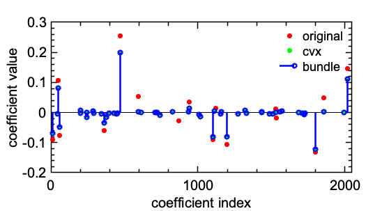
Figure V.1: The coefficients of the original signal and the signals recovered by cvx and by bundle.

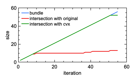
Figure V.2: Size of bundle and its intersection with the atomic support for both original signal and signal recovered by cvx.

V-B Phase retrieval

Phase retrieval is a problem of recovering signal from magnitude-only measurements. Specifically, let $x_{0}\in\mathbb{R}^{n}$ be some unknown signal and the measurements are given by $b_{i}=|\langle x_{0},m_{i}\rangle|^{2}$, where each vector $m_{i}$ encodes illumination $i=1,\ldots,m$. Candés et al. [19] advocate “lifting” the signal as $X_{0}=x_{0}x_{0}^{T}$ so that the measurements are linear in $X_{0}$:

$$b_{i}=\langle x_{0}x_{0}^{T},m_{i}m_{i}^{T}\rangle=\langle X_{0},M_{i}\rangle,\;i=1,\dots,k,$$

where $M_{i}=m_{i}m_{i}^{T}$. The following semidefinite program can be used to recover $X^{*}\approx x_{0}x_{0}^{T}$:

$$\begin{array}[]{ll}\displaystyle\mathop{\hbox{minimize}}_{X}&\operatorname{tr}(X)+\delta_{\succeq 0}(X)\\ \mathop{\hbox{subject to}}&\langle X,M_{i}\rangle=b_{i},\;i=1,\dots,m.\end{array}$$ (V.3)

Define $\mathcal{A}$ as the set of normalized positive semidefinite rank-1 matrices, and define the linear operator $M$ as

$$M(X)=\left[\langle X,M_{i}\rangle\right]_{i=1,\ldots,m}.$$ (V.4)

Then the atomic pursuit problem (II.3) is equivalent to (V.3) with $\mathcal{B}=\{b\}$. The corresponding gauge dual problem is

$$\mathop{\hbox{minimize}}_{y\in\mathbb{R}^{m}}\enspace\enspace\max\set{0,\lambda_{\max}(M^{*}y)}\enspace\mathop{\hbox{subject to}}\enspace\langle b,y\rangle\geq 1,$$ (V.5)

where the adjoint operator $M^{*}$ applied to a vector $y$ is defined as

$$M^{*}y=\sum\limits_{i=1}^{m}y_{i}M_{i}.$$

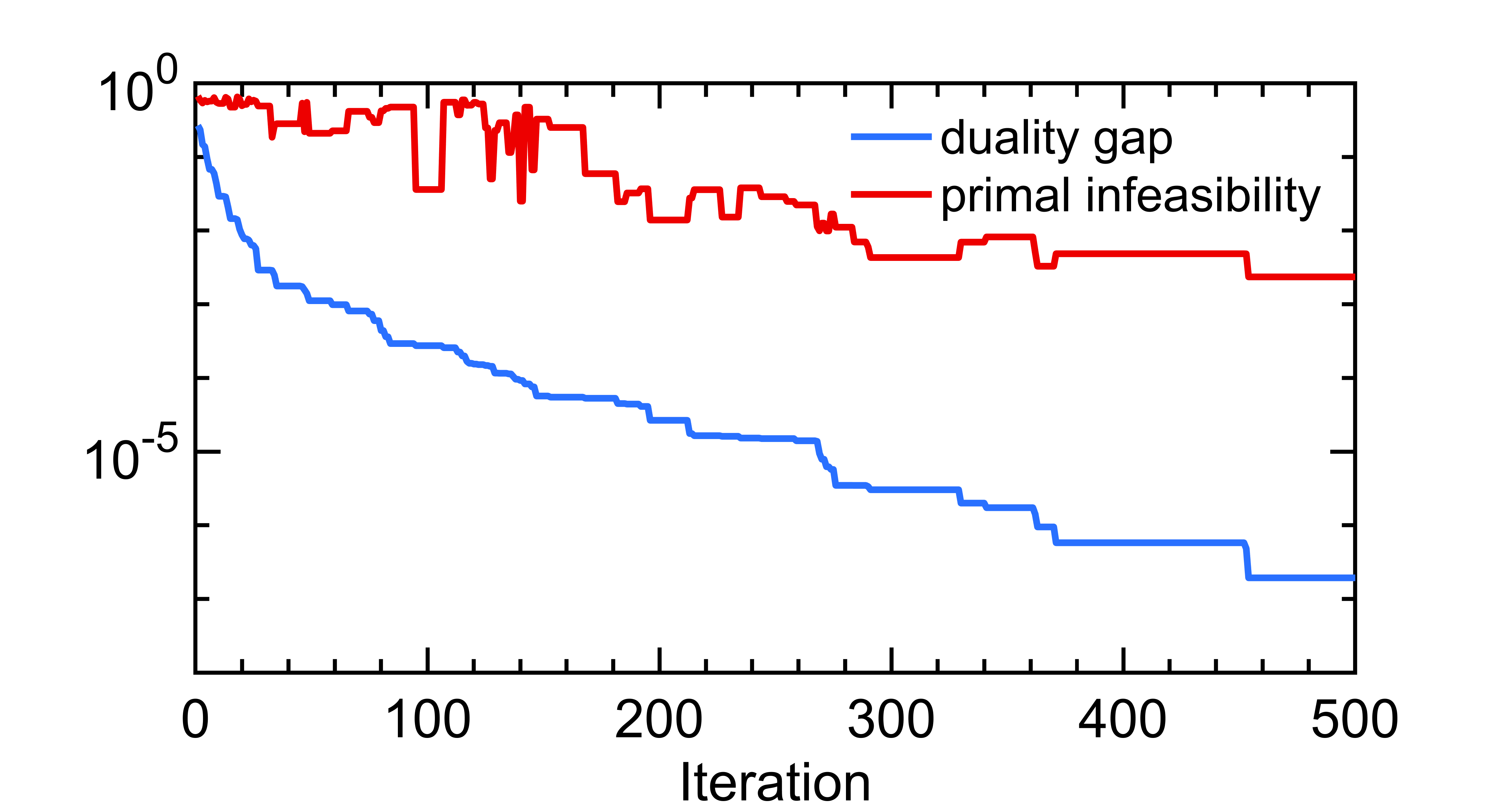
Figure V.3: Convergence of objective value and primal infeasibility.

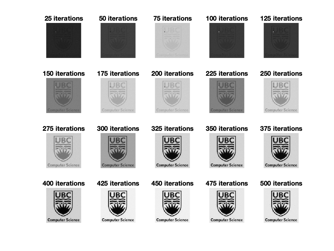
Figure V.4: Images recovered at intermediate iterations of the spectral bundle method for recovering a ground-truth image.

VI Conclusion

Convex optimization formulations of inverse problems often come with very strong recovery guarantees, but the formulations may be too large to be practical for large problems. This is especially true of spectral problems, which require very expensive computational kernels. Our atomic pursuit approach shifts the focus from the solution of the full convex optimization problem to a sequence of “reduced” problems meant to expose the constituent atoms that form the final solution. In some sense, atomic pursuit is a generalization of more classical active-set algorithms. Future avenues of research include the design of specialized SDP solvers for the solution of the highly-structured bundle subproblems, and applying the algorithm framework to other atomic sets.

Appendix A Proofs

A-A Proof for Theorem III.1

Proof:

Let $\mathcal{S}\in\operatorname{\hbox{\rm{supp}}}_{\scriptscriptstyle\mathcal{A}}(x)$. It follows from (II.2) that there exist strictly positive numbers $\set{c_{a}}{a\in\mathcal{S}}$ such that

$$x^{*}=\sum_{a\in\mathcal{S}}c_{a}a\quad\mbox{and}\quad\gamma_{\scriptscriptstyle\mathcal{A}}(x)=\sum_{a\in\mathcal{S}}c_{a},$$

Let $\hat{x}=x/\gamma_{\scriptscriptstyle\mathcal{A}}(x)$ be a normalized solution. Then

$$\hat{x}=\sum_{a\in\mathcal{S}}\frac{c_{a}}{\gamma_{\scriptscriptstyle\mathcal{A}}(x)}a\quad\mbox{and}\quad\gamma_{\scriptscriptstyle\mathcal{A}}(\hat{x})=\sum_{a\in\mathcal{A}}\frac{c_{a}}{\gamma_{\scriptscriptstyle\mathcal{A}}(x)}\equiv 1.$$

This implies that $\hat{x}$ is necessarily a strict convex combination of every point in $\mathcal{S}$. Thus in order to establish that $\mathcal{S}\subseteq\mathcal{F}_{\!\!\scriptscriptstyle\mathcal{A}}(M^{*}y)$, it is sufficient to show $\hat{x}\in\mathcal{F}_{\!\!\scriptscriptstyle\mathcal{A}}(M^{*}y)$. By strong duality,

$$\langle\hat{x},M^{*}y\rangle=\sigma_{\scriptscriptstyle\mathcal{A}}(M^{*}y),$$

and it follows from the definition of exposed faces that $\hat{x}\in\mathcal{F}_{\!\!\scriptscriptstyle\mathcal{A}}(M^{*}y^{*})$. ∎

A-B Proof for Proposition IV.1

Proof:

By the definition of subdifferential of support functions, we have

$$f^{(k)}(z) = \max\limits_{j=1,\dots,k}\sigma_{\scriptscriptstyle\mathcal{A}}(z^{(j)})+\langle a^{(j)},z-z^{(j)}\rangle$$

$$= \max\limits_{j=1,\dots,k}\langle a^{(j)},z\rangle$$

$$= \sigma_{\mathcal{A}^{(k)}}(z).$$

∎

A-C Proof for Proposition IV.1

Proof:

By the definition of subdifferential of support functions, we have

$$f^{(k)}(z) = \max\limits_{j=1,\dots,k}\sigma_{\scriptscriptstyle\mathcal{A}}(z^{(j)})+\langle a^{(j)},z-z^{(j)}\rangle$$

$$= \max\limits_{j=1,\dots,k}\langle a^{(j)},z\rangle$$

$$= \sigma_{\mathcal{A}^{(k)}}(z).$$

∎

A-D Proof for Theorem IV.3

Proof:

• When $\delta>0$, by strong duality( LABEL:prop-support-properties-strong-duality), we know that

  $$\sigma_{\scriptscriptstyle\mathcal{A}}(M^{*}y^{*})\gamma_{\scriptscriptstyle\mathcal{A}}(x^{*}) =1,$$

  $$\sigma_{\hat{\mathcal{A}}}(M^{*}\hat{y})\gamma_{\hat{\mathcal{A}}}(\hat{x}) =1.$$

  Then it follows that,

  $$\gamma_{\hat{\mathcal{A}}}(\hat{x})-\gamma_{\scriptscriptstyle\mathcal{A}}(x^{*}) = \frac{1}{\sigma_{\hat{\mathcal{A}}}(M^{*}\hat{y})}-\frac{1}{\sigma_{\scriptscriptstyle\mathcal{A}}(M^{*}y^{*})}$$

  $$= \frac{\sigma_{\scriptscriptstyle\mathcal{A}}(M^{*}y^{*})-\sigma_{\hat{\mathcal{A}}}(M^{*}\hat{y})}{\sigma_{\hat{\mathcal{A}}}(M^{*}\hat{y})\sigma_{\scriptscriptstyle\mathcal{A}}(M^{*}y^{*})}$$

  $$\leq \frac{\epsilon}{d^{*}(d^{*}-\epsilon)}.$$

  Now by the fact that $\gamma_{\hat{\mathcal{A}}}(\hat{x})\geq\gamma_{\scriptscriptstyle\mathcal{A}}(\hat{x})\geq\gamma_{\scriptscriptstyle\mathcal{A}}(x^{*})$, we can conclude that

  $$\gamma_{\scriptscriptstyle\mathcal{A}}(\hat{x})-\gamma_{\scriptscriptstyle\mathcal{A}}(x^{*})\leq\dfrac{\epsilon}{d^{*}(d^{*}-\epsilon)}.$$

• When $\delta=0$, first, we show that the algorithm will terminate in finite steps with stopping criteria 2. Define

  $$S^{(k)}_{\delta}=\{a\in\mathcal{A}\mid\langle a,M^{*}y_{k}\rangle\geq d^{*}-\delta\}.$$

  By Theorem IV.2, we know that $y^{(k)}\to y^{*}$, where $y^{*}$ is some optimal solution to (III.1). Then there exist positive number $K$ such that $\forall k\geq K$,

  $$\mathcal{F}_{\!\!\scriptscriptstyle\mathcal{A}}(M^{*}y^{*})\subseteq S^{(k)}_{\delta}.$$

  And by the construction of $\mathcal{A}^{(k+1)}$, we know that $\mathcal{A}^{(k+1)}\subseteq S^{(k)}_{\delta}$ for all $k$. We can thus conclude that there exist some finite number $T$ such that $\mathcal{A}_{T+1}=\mathcal{A}_{T}$.

  Next, we show that when the algorithm terminate, the bundle will contain $\operatorname{\hbox{\rm{supp}}}_{\scriptscriptstyle\mathcal{A}}(x^{*})$. From the discussion above, we know that

  $$\mathcal{A}_{T}=S^{(T)}_{\delta}\quad\mbox{and}\quad\mathcal{F}_{\!\!\scriptscriptstyle\mathcal{A}}(M^{*}y^{*})\subseteq S^{(T)}_{\delta}.$$

  Then by Theorem III.1, the result follows.

∎

A-E Proof for Proposition IV.4

Proof:

$$\sigma_{\mathcal{A}^{(k)}}(M^{*}y)$$

$$= \max\bigg{\{}\langle M^{*}y,\alpha W^{(k)}+P^{(k)}V{P^{(k)}}^{T}\rangle\mid$$

$$\quad\alpha\geq 0,\alpha+\operatorname{tr}(V)\leq 1,V\succeq 0\bigg{\}}$$

$$= \max\limits_{0\leq\alpha\leq 1}\bigg{\{}\alpha\langle W^{(k)},M^{*}y\rangle+(1-\alpha)$$

$$\quad\max\{\langle P^{(k)}V{P^{(k)}}^{T},M^{*}y\rangle\mid\operatorname{tr}(V)\leq 1,V\succeq 0\}\bigg{\}}$$

$$= \max\limits_{0\leq\alpha\leq 1}\bigg{\{}\alpha\langle W^{(k)},M^{*}y\rangle+$$

$$\quad(1-\alpha)\max\set{0,\lambda_{\max}({P^{(k)}}^{T}M^{*}yP^{(k)})}\bigg{\}}$$

$$= \max\set{0,\lambda_{\max}({P^{(k)}}^{T}M^{*}yP_{k}),\langle W^{(k)},M^{*}y\rangle}$$

∎

References

- [1] B. Recht, W. Xu, and B. Hassibi, “Necessary and sufficient conditions for success of the nuclear norm heuristic for rank minimization,” in 2008 47th IEEE Conference on Decision and Control. IEEE, 2008, pp. 3065–3070.
- [2] D. Donoho, “For most large underdetermined systems of linear equations the minimal -norm solution is also the sparsest solution,” Communications on pure and applied mathematics, vol. 59, no. 6, pp. 797–829, 2006.
- [3] E. Candes, J. Romberg, and T. Tao, “Robust uncertainty principles: Exact signal reconstruction from highly incomplete frequency information,” arXiv preprint math/0409186, 2004.
- [4] B. Recht, M. Fazel, and P. A. Parrilo, “Guaranteed minimum-rank solutions of linear matrix equations via nuclear norm minimization,” SIAM review, vol. 52, no. 3, pp. 471–501, 2010.
- [5] V. Chandrasekaran, B. Recht, P. A. Parrilo, and A. S. Willsky, “The convex geometry of linear inverse problems,” Foundations of Computational mathematics, vol. 12, no. 6, pp. 805–849, 2012.
- [6] F. F. Bonsall, “A general atomic decomposition theorem and banach’s closed range theorem,” The Quarterly Journal of Mathematics, vol. 42, no. 1, pp. 9–14, 1991.
- [7] D. Amelunxen, M. Lotz, M. B. McCoy, and J. A. Tropp, “Living on the edge: Phase transitions in convex programs with random data,” Information and Inference: A Journal of the IMA, vol. 3, no. 3, pp. 224–294, 2014.
- [8] M. P. Friedlander, I. Macedo, and T. K. Pong, “Gauge optimization and duality,” SIAM Journal on Optimization, vol. 24, no. 4, pp. 1999–2022, 2014.
- [9] A. Y. Aravkin, J. V. Burke, D. Drusvyatskiy, M. P. Friedlander, and K. MacPhee, “Foundations of gauge and perspective duality,” arXiv preprint arXiv:1702.08649, 2017.
- [10] J. E. Kelley, Jr, “The cutting-plane method for solving convex programs,” Journal of the society for Industrial and Applied Mathematics, vol. 8, no. 4, pp. 703–712, 1960.
- [11] C. Lemaréchal, A. Nemirovskii, and Y. Nesterov, “New variants of bundle methods,” Mathematical programming, vol. 69, no. 1-3, pp. 111–147, 1995.
- [12] K. C. Kiwiel, “Proximity control in bundle methods for convex nondifferentiable minimization,” Mathematical programming, vol. 46, no. 1-3, pp. 105–122, 1990.
- [13] J. B. Cruz and W. de Oliveira, “Level bundle-like algorithms for convex optimization,” Journal of Global Optimization, vol. 59, no. 4, pp. 787–809, 2014.
- [14] U. Brännlund, K. C. Kiwiel, and P. O. Lindberg, “A descent proximal level bundle method for convex nondifferentiable optimization,” Operations Research Letters, vol. 17, no. 3, pp. 121–126, 1995.
- [15] C. Helmberg and F. Rendl, “A spectral bundle method for semidefinite programming,” SIAM Journal on Optimization, vol. 10, no. 3, pp. 673–696, 2000.
- [16] M. P. Friedlander and I. Macedo, “Low-rank spectral optimization via gauge duality,” SIAM Journal on Scientific Computing, vol. 38, no. 3, pp. A1616–A1638, 2016.
- [17] L. Ding, A. Yurtsever, V. Cevher, J. A. Tropp, and M. Udell, “An optimal-storage approach to semidefinite programming using approximate complementarity,” arXiv preprint arXiv:1902.03373, 2019.
- [18] S. S. Chen, D. L. Donoho, and M. A. Saunders, “Atomic decomposition by basis pursuit,” SIAM review, vol. 43, no. 1, pp. 129–159, 2001.
- [19] E. J. Candes, Y. C. Eldar, T. Strohmer, and V. Voroninski, “Phase retrieval via matrix completion,” SIAM review, vol. 57, no. 2, pp. 225–251, 2015.