Automatic Testing With
Reusable Adversarial Agents

Abstract

Autonomous systems such as self-driving cars and general-purpose robots are safety-critical systems that operate in highly uncertain and dynamic environments. We propose an interactive multi-agent framework where the system-under-design is modeled as an ego agent and its environment is modeled by a number of adversarial (ado) agents. For example, a self-driving car is an ego agent whose behavior is influenced by ado agents such as pedestrians, bicyclists, traffic lights, road geometry etc. Given a logical specification of the correct behavior of the ego agent, and a set of constraints that encode reasonable adversarial behavior, our framework reduces the adversarial testing problem to the problem of synthesizing controllers for (constrained) ado agents that cause the ego agent to violate its specifications. Specifically, we explore the use of tabular and deep reinforcement learning approaches for synthesizing adversarial agents. We show that ado agents trained in this fashion are better than traditional falsification or testing techniques because they can generalize to ego agents and environments that differ from the original ego agent. We demonstrate the efficacy of our technique on two real-world case studies from the domain of self-driving cars.

I Introduction

Autonomous cyber-physical systems such as self-driving vehicles and unmanned aerial vehicles operate in highly uncertain environments. For such systems, it is imperative to develop a testing framework where the system-under-design (SUD) is exposed to challenging scenarios posed by its operating environment. The view we adopt in this paper is that an autonomous system and its environment can be modeled as an interactive multi-agent system, where the SUD is the ego agent and the environment can be viewed as a composition of several ado agents. For example, when designing software for a self-driving car, the car itself is the ego agent, while aspects such as other vehicles, pedestrians, traffic lights, road markings, road curvature, and weather (among others) can be considered as ado agents capable of autonomous behavior. The main goal of an adversarial testing procedure is to find behaviors presented by the ado agents that induce an undesired behavior by the ego agent. An interesting challenge is that unrestricted ado agents can lead to trivial violations of the ego agent’s specification. For example, in the self-driving domain, consider an ego vehicle following an ado car on a highway; a reasonable assumption is that the ado car does not travel backward and that it follows traffic laws. Thus, the goal of adversarial testing is actually to find violations of the ego agent behavior subject to a set of constrained ado agents.

There is significant existing work that addresses adversarial testing. The most prominent class of techniques focuses on requirement falsification [1, 2, 3, 4, 5] ; here, we assume that the SUD is a black-box model with time-varying inputs and outputs, and its correctness specification is expressed as a Signal Temporal Logic (STL) property of the outputs. Various black-box optimization heuristics are used to search over the (constrained) space of the model inputs to identify a violation of the output property (See [6] for a survey). Search-based testing [7] is another set of related techniques that rely on heuristic search. Search-based testing and falsification are fundamentally limited; these are non-adaptive approaches, i.e., a counterexample is a fixed sequence of actions undertaken by the environment (i.e. ado agents) which does not generalize to new initial conditions for the agents or to changes in the dynamics of the system. Thus, any change in the ego agent or the environment necessitates re-running the falsification/search-based testing tools, which is time-consuming in iterative design flows.

The recently developed adaptive stress testing (AST) approach [8, 9] takes a different approach. It uses a multi-agent view similar to the one we adopt in this paper to find undesired behavior in ego agents. The goal in AST is not to find a single (or a set of) counterexamples, but rather to learn an adversarial policy (using reinforcement learning (RL)) that causes the ego agent to fail. In this paper, we significantly extend the AST idea in several ways. To better contextualize our contributions, we use a motivating example.

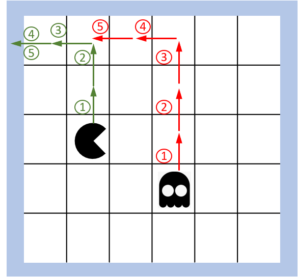
Figure 1: Ego agent (pacman) evading adversarial agent (ghost)

Motivating Example. Consider two agents moving in a grid-world as shown in Fig. 1, where at each time step, the ego agent moves one step in a direction away from the the adversary. If it picks a direction that has a grid boundary (wall), then it fails to move. We say that the “ego is $r$-captured by the ado” if the Manhattan distance (denoted $d_{\mathrm{man}}$) between the grid cells occupied by the ego (denoted $c_{\mathsf{ego}}$) and the ado (denoted $c_{\mathsf{ado}}$) is less than the positive integer $r$. In temporal logic, we can express the property that the ego not be captured for at least $k$ time steps as ${\psi_{\mathsf{ego}}}$ $\equiv$ $\mathbf{G}_{[0,k]}\left(d_{\mathrm{man}}(c_{\mathsf{ego}},c_{\mathsf{ado}})>r\right)$. The goal is to find ado behavior that makes the ego violate this property. Consider a motion model in which the ado agent can instantaneously jump to the location of the ego agent – clearly this is a trivial policy that ensures that the ego violates ${\psi_{\mathsf{ego}}}$, but this may not be reasonable behavior for the ado agent. Thus, there may be a need to restrict the behaviors that the ado agent can have, and such constraints can also be expressed using temporal logic. In this example, the constraint ${\varphi_{\mathsf{ado}}}$ $\equiv$ $\mathbf{G}_{[0,k]}\left(\left|\left|v_{\mathsf{ado}}\right|\right|_{\infty}\leq 1\right)$ restricts the maximum velocity of the ado in either the X or Y direction to be less than 1.

Traditional testing tools [1, 2] treat falsification as a search problem over a user-defined parameter space. For example, the user can introduce $N$ parameters for the $N$-length sequence of actions picked by the ado agent. The space of actions $A$ can be discrete or continuous, and essentially the falsification problem tries to find one sequence in $A^{N}$ such that the ego violates ${\psi_{\mathsf{ego}}}$. Fig 1 demonstrates such a sequence: the ado travels upward 3 times and to the left twice, while the ego gets trapped in the top left corner. A sequence found by such a tool is however, not generalizable: suppose the ego was already in the top left corner, and the ado was in the bottom right corner, then blindly following the sequence (3 ups and 2 lefts) does not lead to a violation of ${\psi_{\mathsf{ego}}}$. Furthermore, if the ego were to allowed to move 2 cells in one time step (instead of 1), then such a fixed sequence will almost certainly not succeed in making the ego violate its spec.

Problem Definition. Given: (1) a formal specification for the ego agent in a suitable temporal logic and a fixed implementation of its control logic, (2) a set of (dynamic) constraints for each of the ado agents (also specified in a suitable temporal logic), and (3) an executable model to simulate the interactions between the agents, the goal of this paper is to identify ado agent behaviors that lead to a violation of the ego specification. Furthermore, we would like the testing strategy to be robust to changes in the ego agent, as outlined in the motivating example.

Solution Overview. While traditional adversarial testing tools focus on searching over the action space of the ado agent(s), we propose a technique to search over the set of mappings from states to actions, or the set of policies for a given ado agent. This can be done by parameterizing the control logic of the ado agents, and using an appropriate controller synthesis procedure to obtain ado policies that lead to ego agent violations. Specifically, we explore the use of reinforcement learning (RL). The work in [9, 8] also uses RL to identify adversarial policies to make the ego agent display undesired behavior. There are several key differences and improvements in our work: (1) In contrast to [9, 8], where state-based rewards to be used by the RL procedure are hand-created, we express both the specification for the ego agent and the dynamic constraints for the ado agents using temporal logic. This allows us to automatically infer the rewards to use in RL allowing us to avoid reward engineering – a required but manual and error-prone step in RL [10]. (2) We show how our algorithms make the testing process robust – our trained ado agents are able to find ego violations even after changes to the ego agent model without having to re-train the ado agent for the perturbed ego agent. Our procedure yields reusable, robust and modular adversarial agents that can reduce the development time in an iterative design process.

Summary of contributions.

1. We formulate a new adversarial testing algorithm for autonomous systems that views the SUD as an ego agent that interacts with a set of constrained ado agents. We assume correctness specification for the ego agent, and the behavioral constraints on the ado agents are expressed in a formal logic such as Linear Temporal Logic (LTL) or Signal Temporal Logic (STL) [11]. We propose a framework where controller synthesis can be used to train an ado agent policy to discover violations of the ego specification, and explore a specific controller synthesis procedure based on deep reinforcement learning. Specifically, we leverage the quantitative semantics of STL to guide the deep RL based ado agent synthesis.

2. We identify assumptions under which the learned ado policies are robust. In particular we show that if the learned ado policy demonstrates a violation of the ego specification, then this policy will discover violations in an ego agent that (1) starts from different initial configurations, and (2) has different dynamics than the original ego agent.

3. We demonstrate the efficacy of our approach on two case-studies from the self-driving domain. We show that aspects such as other cars, traffic lights, pedestrians, etc. can be modeled as ado agents. We consider (1) an adaptive cruise control example where the leading car is modeled as an ado agent, and (2) a controller that ensures safety during an ado car merging into an ego car’s lane.

The rest of the paper is organized as follows. In Section II we provide the background and problem definition. We define rewards to be used by our RL-based testing procedure in Sec. III. We show how the ado agents generalize in Section IV, and provide detailed evaluation of our technique in Sec. V. Finally, we conclude with a discussion on related work in Section VI.

II Problem Statement and Background

We first introduce the formal description of a multi-agent system as a collection of deterministic dynamical agents.

Definition 1 (Deterministic Dynamical Agents).

An agent $\mathcal{H}$ is a tuple $(X,A,T,{X_{\mathrm{init}}},\pi)$, where $X$ is a set of agent states, $A$ is the set of agent actions, $T$ is a set of transitions of the form $(\mathbf{x},a,\mathbf{x}^{\prime})$, where $a\in A$, ${X_{\mathrm{init}}}\subseteq X$ is a set of designated initial states for the agent, and finally the policy $\pi$ is a function mapping a state in $X$ to an action in $A$.

A multi-agent system $\mathcal{S}=\{\mathsf{ego},\mathsf{ado}_{1},\ldots,\mathsf{ado}_{k}\}$ is a set of agents, with a designated ego agent $\mathsf{ego}$, and a non-empty set of adversarial agents $\mathsf{ado}_{1},\ldots,\mathsf{ado}_{k}$. The state-space of the multi-agent system can be constructed as a product space of the individual agent state spaces, and the set of transitions of the multi-agent system corresponds to the synchronous product of the transitions of individual agents. The transitions of the multi-agent system when projected to individual agents are consistent with individual agent behaviors. A behavior trajectory for an agent is thus a finite or infinite sequence $(t_{0},\mathbf{x}_{0}),(t_{1},\mathbf{x}_{i}),\ldots$, where $\mathbf{x}_{i}\in X$ and $t_{i}\in\mathbb{R}^{\geq 0}$. We use $s$ to denote a trajectory variable, i.e. a function mapping $t_{i}$ to $\mathbf{x}_{i}$, i.e. $s(t_{i})=\mathbf{x}_{i}$. In many frameworks used for simulating multi-agent systems, it is common to consider timed trajectories with a finite time horizon $t_{N}$, and a fixed, discrete time step, $\Delta=t_{i+1}-t_{i},\forall i$.

Signal Temporal Logic. Signal Temporal Logic (STL) [11] is a formalism to describe properties of real-valued, dense-time trajectories. STL formulas are evaluated over behavior trajectories. An atomic STL formula is a predicate of the form $f(s)\sim c$, where $s$ is a trajectory variable, $f$ is a real-valued function from $X$ to $\mathbb{R}$, $\sim$ is a comparison operator, i.e. $\sim\in\{<,\leq,>,\geq\}$ and $c\in\mathbb{R}$. STL formulas are constructed recursively using the Boolean logical connectives such as negations ($\neg$) and conjunctions ($\wedge$) and the temporal operator ($\mathbf{U}$). It is often convenient to define Boolean connectives such as disjunction ($\vee$), implication ($\Rightarrow$) using the usual equivalences for Boolean logic. It is also convenient to define temporal operators $\mathbf{F}_{I}\varphi$ as shorthand for $\top\mathbf{U}_{I}\varphi$, and $\mathbf{G}_{I}\varphi$ as shorthand for $\neg\mathbf{F}_{I}\neg\varphi$. Each temporal operator is indexed by the time interval $I$ of the form $[a,b]$, where $a,b\in\mathbb{R}^{\geq 0}$.

STL has both Boolean semantics that recursively define the truth value of the satisfaction of an STL formula in terms of the satisfaction of its subformulas and quantitative semantics that are used to map a trajectory and a formula to a real value known as the robust satisfaction value or simply, the robustness. Intuitively, the robustness approximates the distance between a given signal $s$ and the set of signals satisfying the formula $\varphi$ [12]. There are numerous definitions for quantitative semantics of STL, for example [13] [14]. The actual definition to be used is irrelevant to this paper as long as it is efficiently computable. We will assume that the robustness has been clamped to be in an interval $[\rho_{min},\rho_{max}]$, with $\rho_{min}=-\rho_{max}>0$

When evaluating an STL formula, each time step requires an application of the functions $f$ that appear in the formula. We denote a signal $s$ satisfying a formula $\varphi$ at time $t$ by $s,t\models\varphi$, and $s\models\varphi$ is by convention defined as $s,0\models\varphi$. In [12, 15], the authors show that $\rho(\varphi,s)\geq 0\implies s\models\varphi$, and $\rho(\varphi,s)<0\implies s\not\models\varphi$. Following the notation in [15], we call the signal variables appearing in the formulas as primary signals, and the intermediate results that arise from function applications as secondary signals.

Definition 2 (Definition 2 of [15]).

Let $f_{k}(s)$ be any arithmetic function $f_{k}:X\rightarrow\mathbb{R}$ that appears in an STL formula $\varphi$. We call the vector of variables in $s$ the primary signals of $\varphi$, and their images by $f$ secondary signals, $\{y_{k}\}$.

Lemma 1 tells us that if two signals have “nearby values” and also generate nearby secondary signals, then if one of them robustly satisfies an STL formula, the other will also satisfy that formula. We first formalize the notion of distance between signals.

Definition 3 (Distance between signals).

Given two signals $s$ and $s^{\prime}$ with identical value domains $S$ and identical time domains $\mathbb{T}$, and a metric $d_{S}$ on $S$, the distance between $s$ and $s^{\prime}$, denoted as $\left|\left|s-s^{\prime}\right|\right|$ is defined as: $\sup_{t\in\mathbb{T}}d_{S}(s(t),s^{\prime}(t))$.

Lemma 1 (Theorem 1 in [15]).

If $\rho(\varphi,s,t)=\delta$, then for every signal $s^{\prime}$ s.t. every secondary signal satisfies $\left|\left|y_{k}-y_{k}^{\prime}\right|\right|<\delta$, then $(s\models\varphi)\implies(s^{\prime}\models\varphi)$.

Problem Definition: Testing with Dynamically Constrained Adversaries. Given a behavior of the multi-agent system, let the projection of the behavior onto agent $\mathcal{H}$ be denoted by the signal variable $s_{\mathcal{H}}$. Formally, the problem we wish to solve can be stated as follows:

1. Given a spec ${\psi_{\mathsf{ego}}}$ on the ego agent,

2. Given a set of constraints ${\varphi_{\mathsf{ado}}}_{i}$ on adversarial agent $\mathcal{H}_{i}$,

3. Find a multi-agent system policy that can generate behaviors such that: $\forall i:s_{\mathsf{ado}_{i}}\models{\varphi_{\mathsf{ado}}}_{i}\wedge s_{\mathsf{ego}}\not\models{\psi_{\mathsf{ego}}}$.

In other words, we aspire to generate a compact representation for a possibly infinite number of counterexamples to the correct operation of the ego agent.

II-A Adversarial Testing through Policy Synthesis

In contrast to falsification approaches, we assume a deterministic (or stochastic) dynamical agent model for the ado agents (as defined in Def.  1), i.e. the $i^{th}$ ado agent is specified as a tuple of the form $(X_{i},A_{i},T_{i},{X_{\mathrm{init}}}_{i},\pi_{i})$. We assume that initially all agents have a randomly chosen policy $\pi_{i}$. For ado agent $\mathsf{ado}_{i}$, let $\Pi_{i}=A_{i}^{X_{i}}$ denotes the set of all possible policies. Let $\Pi_{i}({\varphi_{\mathsf{ado}}}{i})$ be the set of policies such that for any $\pi\in\Pi_{i}({\varphi_{\mathsf{ado}}}{i})$, using $\pi$ guarantees that the sequence of states of $\mathsf{ado}_{i}$ satisfies ${\varphi_{\mathsf{ado}}}_{i}$. Similarly, let $\Pi_{i}(\neg{\psi_{\mathsf{ego}}})$ be the set of policies that guarantees that the sequence of states for the ego agent $\mathsf{ego}$ does not satisfy ${\psi_{\mathsf{ego}}}$. The problem we wish to solve is: for each $i$, find a policy in $\Pi_{i}(\neg{\psi_{\mathsf{ego}}})\cap\Pi_{i}({\varphi_{\mathsf{ado}}}{i})$.

One approach to solve this problem is to use a reactive synthesis approach, when specifications are provided in a logic such as LTL or ATL [16, 17, 18]. There is limited work on reactive synthesis with STL objectives [19, 20], mainly requiring encoding STL cosntraints as Mixed-Integer Linear Programs; this may suffer from scalability in multi-agent settings. We defer detailed comparison with reactive synthesis approaches to future work. In this paper, we propose using the framework of deep reinforcement learning (RL) for controller synthesis with a procedure for automatically inferring rewards from specifications and constraints.

II-B Policy synthesis through Reinforcement Learning

Reinforcement learning (RL) [21] and related deep reinforcement learning (DRL) [22] are procedures to train agent policies in deterministic or stochastic environments. In our setting, given a multiagent system $\mathcal{S}=\{\mathsf{ego},\mathsf{ado}_{1},\dots,\mathsf{ado}_{k}\}$, we wish to synthesize a policy $\pi_{k}$ for each ado $\mathsf{ado}_{k}$. We can model multiple ado agents as a single agent whose state is an element of the Cartesian product of the state spaces of all agents, i.e., $X=X_{\mathsf{ego}}\times X_{\mathsf{ado}_{1}}\times\dots\times X_{\mathsf{ado}_{k}}$, and the action of this single agent is a a tuple of actions of all ado agents, i.e. $A=A_{\mathsf{ado}_{1}}\times\ldots\times A_{\mathsf{ado}_{k}}$.

In each step, we assume that the agent is in state $\mathbf{x}\in X$ and interacts with the environment by taking action $a\in A$. In response, the environment (i.e. the transition relation of the ado and the ego agents) picks a next state $\mathbf{x}^{\prime}$ s.t. $(\mathbf{x},a,\mathbf{x}^{\prime})\in T$, and a reward $R(\mathbf{x},a)$. The reward provides reinforcement for the constrained adversarial behavior, and will be elaborated in Section III. The goal of the RL agent is to learn a deterministic policy $\pi(\mathbf{x})$, such that the long term payoff of the agent from the initial state (i.e. the discounted sum of all rewards from that state) is maximized. As is common in RL, we define the notion of a value function $V$ in Eq. (1); this is the expected reward over all possible actions that may be taken by the agent. In a deterministic environment, the expectation disappears.

$$V_{\pi}(\mathbf{x}_{t})=\mathbb{E}_{\pi}\left[\begin{array}[]{ll}\displaystyle\sum_{k=0}^{\infty}&\gamma^{k}R((\mathbf{x}_{t+k}),a_{t+k})\ \Bigg{\lvert}a_{t+k}=\pi(\mathbf{x}_{t+k})\end{array}\right]$$ (1)

RL algorithms use different strategies to find an optimal policy $\pi*$, that for all $\mathbf{x}$ is defined as $\pi^{*}(\mathbf{x})=\operatorname*{arg\,max}_{\pi}V_{\pi}(\mathbf{x})$. We assume that the state of the agent at time $t_{0}$, i.e. $\mathbf{x}_{0}$ is in ${X_{\mathrm{init}}}$.

We now briefly review a classic model-free RL algorithm called q-learning and summarize two deep RL algorithms: Deep Q-learning and Proximal Policy Optimization (PPO). In q-learning, we learn a state-action value function $q(\mathbf{x},a)$, which represents the believed value of taking action $a$ when in state $\mathbf{x}$. Note that $V(\mathbf{x})=\max_{a}q(\mathbf{x},a)$. In q-learning, the agent maintains a table whose rows correspond to the states of the system and columns correspond to the actions. The entry $q(\mathbf{x},a)$, encodes an approximation to the state-action value function computed by the algorithm. The table is initialized randomly. At each time step $t$, the agent uses the table to select an action $a_{t}$ based on an $\varepsilon$-greedy policy, i.e. it chooses a random action with probability $\varepsilon$, and with probability $1-\varepsilon$, chooses $\text{argmax}_{a\in A}q(\mathbf{x},a)$. Next, at time step $t+1$, the agent observes the reward received $R_{t+1}$ as well as the new state $\mathbf{x}_{t+1}$, and it uses this information to update its beliefs about its previous behavior. During the training process, we sample the initial state of each episode with a probability distribution $\mu(\mathbf{x})$ that is nonzero at all states. Given enough time, all states will eventually be selected as the initial state. We also fix the policies of the ado agents to be $\varepsilon$-soft. This means that for each state $\mathbf{x}$ and every action $a$, $\pi(a|x)\geq\varepsilon$, where $\varepsilon>0$ is a parameter. Together, random sampling of initial states and $\varepsilon$-soft policies ensure that the agent performs sufficient exploration and avoids converging prematurely to local optima.

Deep RL. Deep RL is a family of algorithms that make use of Deep Neural Networks (DNNs) to represent either the value or the policy of an agent. Deep Q-learning [22], is an extension of q-learning where the table $q(s,a)$ is approximated by a DNN, $q(s,a,w)$, where $w$ are the network parameters. Deep Q-learning observes states and selects actions similarly to Q-learning, but it additionally uses experience replay, in which the agent stores previously observed tuples of states, actions, next states, and rewards. At each time step, the agent updates its q-function with the currently observed experience as well as with a batch of experiences sampled randomly from the experience replay buffer. The agent then updates its approximation network by gradient descent on the quadratic loss function $\mathcal{L}=(y_{t}-q(\mathbf{x}_{t},a_{t},w))^{2}$, where $y_{t}=R_{t+1}+\gamma\max_{a^{\prime}}q(\mathbf{x}_{t+1},a,w).$ In the case that $\mathbf{x}_{t}$ is a terminal state, it is common to assume that all transitions are such that $\mathbf{x}_{t+1}=\mathbf{x}_{t}$ and $R_{t}=0$. Although these learning algorithms learn the state-action value function $q(\mathbf{x},a)$, in the theoretical exposition that follows, we will use the state value function $V(\mathbf{x})$ for simplicity. The optimal state value function can be obtained from the optimal state-action value function by $V^{\star}(\mathbf{x})=\max_{a}q^{\star}(\mathbf{x},a)$. PPO [23] is a state-of-the-art policy gradient algorithm that performs gradient-based updates on the policy space directly while ensuring that the new policy is not too far from the old policy.

III Learning Constrained Adversarial Agents

In this section, we describe how we construct a reward function that enables training constrained adversarial agents. Note that the reward function needs to encode two aspects: (1) satisfying ado constraints, (2) violating ego specification. We assume that ado constraints are hierarchically ordered with priorities, inspired by the Responsibility-Sensitive Safety rules for traffic scenarios in [24].

Definition 4 (Constrained adversarial reward).

Suppose from initial state $\mathbf{x}_{0}$ the agent has produced a behavior trace $s(\mathbf{x}_{0})$ of duration $T$. We distinguish two cases.

• Case 1: All ado constraints are strictly satisfied, i.e. $\rho(c,s(\mathbf{x}_{0}))>0$ for each constraint $c\in{\varphi_{\mathsf{ado}}}$. In this case, the reward will be the robustness of the adversarial specification.

  $$R_{t}=\left\{\begin{array}[]{ll}0&\text{if $t<T$}\\ \rho(\neg{\psi_{\mathsf{ego}}},s(\mathbf{x}_{0}))&\text{ if $t=T$}\end{array}\right.$$ (4)

• Case 2: Not all ado constraints are strictly satisfied. Let $c$ be the highest priority rule that is not strictly satisfied, i.e. the highest priority rule such that $\rho(c,s(\mathbf{x}_{0}))\leq 0$. Then, every constraint with priority higher than $c$ will contribute zero, whereas every constraint with priority less then or equal to $c$ will contribute $\rho_{min}$. Let $M$ be the number of constraints with priority less than or equal to $c$.

  $$R_{t}=\left\{\begin{array}[]{ll}0&\text{if $t<T$}\\ -M\rho_{min}&\text{if $t=T$}\end{array}\right.$$ (7)

The following lemma shows that it is not possible for an ado agent to attain a high reward for satisfying lower priority constraints at the expense of higher priority constraints. The proof is straightforward (shown in the appendix).

Lemma 2 (Soundness of the reward function).

Consider two traces, $s_{1}$ and $s_{2}$. Suppose that the highest priority constraint violated by $s_{1}$ is $c_{1}$ and the highest priority constraint violated by $s_{2}$ is $c_{2}$. Suppose $c_{1}$ has lower priority than $c_{2}$. Then, the reward for trajectory 1 will be higher than the reward for trajectory 2, i.e. $R(s_{1})>R(s_{2})$.

IV Generalizability of Adversarial Agents

In this section we show how our RL-based testing approach makes the testing procedure itself robust by learning a closed-loop policy for testing. We first show generalizability across initial conditions in two steps: (1) In Theorem 1, we assume that the RL algorithm has converged to the optimal value function, and that it has used this value function to find a counterexample trace $s(\mathbf{x}_{0})$. We consider a new state $\mathbf{x}_{0}^{\prime}$, and want to bound the degradation of the robustness function of the specification $\rho(\neg{\psi_{\mathsf{ego}}},s(\mathbf{x}_{0}^{\prime}))$. (2) In Theorem 2, we relax this strong assumption and identify conditions under which generalization can be guaranteed even with approximate convergence. In Theorem 3, we show generalizability when the ego agent dynamics change. The main idea is that if the new dynamics have an $\epsilon$-approximate bisimulation relation to the original dynamics, then we can guarantee generalizability.

Theorem 1.

Suppose that the adversarial agent has converged to the optimal value function $V^{\star}(\mathbf{x})$, and that it has found a trace $s(\mathbf{x}_{0})$ that falsifies the target specification ${\psi_{\mathsf{ego}}}$ with robustness $\rho(\neg{\psi_{\mathsf{ego}}},s(\mathbf{x}_{0}))=\tau>0$ while satisfying all of the ado constraints. Given a new state $\mathbf{x}_{0}^{\prime}$ such that $\left|V^{\star}(\mathbf{x}_{0})-V^{\star}(\mathbf{x}_{0}^{\prime})\right|<\delta$ with $\delta<\gamma^{T}|\rho_{min}|$, the adversary will be able to find a new trajectory $s(\mathbf{x}_{0}^{\prime})$ that satisfies all of the constraints. Furthermore, the robustness of the specification $\neg{\psi_{\mathsf{ego}}}$ over the new trace will be at least $\tau-\delta/\gamma^{T}$.

Proof.

We can expand the optimal value function at state $\mathbf{x}_{0}$ as $V^{\star}(\mathbf{x}_{0})=\sum_{t=0}^{T}\gamma^{t}R_{t}$, where $R_{t}$ is the reward function defined in Definition 4. Then, the optimal value function at $\mathbf{x}_{0}$ is $V^{\star}(\mathbf{x}_{0})=\gamma^{T}\tau$. Suppose for a contradiction that the new trajectory $s(\mathbf{x}_{0}^{\prime})$ violates some number $M$ of constraints. Then, the following equations show that the two states must actually differ by a large amount, much larger than $\delta$, leading to a contradiction. Formally, from Definition 4 we have

$$V^{\star}(\mathbf{x}_{0}^{\prime}) =-\gamma^{T}M\rho_{min},$$ (8)

$$\left|V^{\star}(\mathbf{x}_{0}^{\prime})-V^{\star}(\mathbf{x}_{0})\right| \geq\gamma^{T}\tau+M\gamma^{T}\rho_{min}>\delta,$$ (9)

which contradicts the assumption of the theorem. As the constraints will be satisfied by $s(\mathbf{x}_{0}^{\prime})$, their contribution to the value function at $\mathbf{x}_{0}^{\prime}$ will be zero. Then, for the $2^{nd}$ part of the theorem we can expand the optimal value function as:

$$\left|V^{\star}(\mathbf{x}_{0})\!-\!V^{\star}(\mathbf{x}_{0}^{\prime})\right|\!=\!\left|\gamma^{T}\rho(\neg{\psi_{\mathsf{ego}}},s(\mathbf{x}_{0}))\!-\!\gamma^{T}\rho(\neg{\psi_{\mathsf{ego}}},s(\mathbf{x}_{0}^{\prime}))\right|$$ (10)

By assumption the above terms are $\leq\delta$, which gives us that

$$\left|\rho(\neg{\psi_{\mathsf{ego}}},s(\mathbf{x}_{0}))-\rho(\neg{\psi_{\mathsf{ego}}},s(\mathbf{x}_{0}^{\prime})))\right|\leq\frac{\delta}{\gamma^{T}}$$ (11)

and the theorem follows. ∎

Note that if $\delta$ is chosen as a small enough perturbation such that $\tau-\delta/\gamma^{T}>0$, then the new trace is also a trace in which the adversary causes the ego to falsify its specification.

The tabular Q-learning algorithm is guaranteed to converge asymptotically to the optimal value function, meaning that for any $\epsilon$, there exists a $k$ such that at the $k$-th iteration, the estimate $V_{k}$ differs from the optimal value function by at most $\alpha$, i.e. $\forall\mathbf{x}\in X$, $\left|V^{\star}(\mathbf{x})-V_{k}(\mathbf{x})\right|<\alpha$. Some RL algorithms have even stronger guarantees. For example, Theorem 2.3 of [25], states that running the value iteration algorithm until iterates of the value function differ by at most $\frac{\alpha(1-\gamma)}{2\gamma}$ produces a value function that converges within $\alpha$ of the value function $\left|V_{k}(\mathbf{x}_{0})-V^{\star}(\mathbf{x}_{0})\right|\leq\alpha$. While useful for theoretical results, value iteration does not scale to problems with large state spaces. The following theorem states that if the RL algorithm has found a value function that is near optimal, the agent will be able to generalize counterexamples across different initial states.

Theorem 2.

Suppose that we have truncated an RL algorithm at iteration $k$. Suppose that, from the guarantees of this particular RL algorithm, we are within $\alpha$ of the optimal value function, i.e. for every $\mathbf{x}$, $\left|V_{k}(\mathbf{x}_{0})-V^{\star}(\mathbf{x}_{0})\right|\leq\alpha$. Further suppose that the adversarial agent has found a falsifying trace from state $\mathbf{x}_{0}$ with robustness $\tau$, i.e. $\rho(\neg{\psi_{\mathsf{ego}}},s(\mathbf{x}_{0}))=\tau$. Now consider a new state $\mathbf{x}_{0}^{\prime}$ such that the degradation of our approximate value function is at most $\beta$, i.e. $\left|V_{k}(\mathbf{x}_{0})-V_{k}(\mathbf{x}_{0}^{\prime})\right|\leq\beta$. Then, the adversarial agent will be able to produce a new trace with robustness at least

$$\rho(\neg{\psi_{\mathsf{ego}}},s(\mathbf{x}_{0}^{\prime}),T)\geq\tau-\frac{2\alpha+\beta}{\gamma^{T}}$$ (12)

Proof.

Note that by the triangle inequality

$$\alpha+\beta> \left|V_{k}(\mathbf{x}_{0})-V^{\star}(\mathbf{x}_{0})\right|+\left|V^{\star}(\mathbf{x}_{0}^{\prime})-V_{k}(\mathbf{x}_{0})\right|$$ (13)

$$> \left|V_{k}(\mathbf{x}_{0}^{\prime})-V^{\star}(\mathbf{x}_{0})\right|$$ (14)

Further,

$$2\alpha+\beta>\left|V_{k}(\mathbf{x}_{0}^{\prime})-V^{\star}(\mathbf{x}_{0})\right|>\left|V^{\star}(\mathbf{x}_{0}^{\prime})-V^{\star}(\mathbf{x}_{0})\right|$$ (15)

The result now follows from Theorem 1 by substituting $\delta=2\alpha+\beta$. ∎

Finally, we will show that the agent may cope with limited changes to the multiagent system. This is useful in a testing and development situation, because we would like to be able to reuse a pre-trained ado to stress-test small modifications of the ego without expensive retraining. To do this, we will define an $\epsilon$-bisimulation relation that will allow us to formally characterize the notion of similarity between different multiagent systems.

Definition 5 ($\epsilon$-approximate bisimulation, [26]).

Let $\epsilon>0$, and $\mathcal{S}_{1}$, $\mathcal{S}_{2}$ be systems with state spaces $X_{1}$, $X_{2}$ and transition relations $T_{1}$, $T_{2}$, respectively. A relation $\mathcal{R}_{\epsilon}\subseteq X_{1}\times X_{2}$ is called an $\epsilon$-approximate bisimulation relation between $T_{1}$ and $T_{2}$ if for all $\mathbf{x}_{1},\mathbf{x}_{2}\in\mathcal{R}_{\epsilon}$,

1. $d(x_{1},x_{2})\leq\epsilon$ where $d$ is a distance metric

2. $\forall a\in A$, $\forall\mathbf{x}_{1}^{\prime}\in T_{1}(\mathbf{x}_{1},a)$, $\exists\mathbf{x}_{2}^{\prime}\in T_{2}(\mathbf{x}_{2},a)$ such that $(\mathbf{x}_{1}^{\prime},\mathbf{x}_{2}^{\prime})\in\mathcal{R}_{\epsilon}$

3. $\forall a\in A$, $\forall\mathbf{x}_{2}^{\prime}\in T_{2}(\mathbf{x}_{2},a)$, $\exists\mathbf{x}_{1}^{\prime}\in T_{1}(\mathbf{x}_{1},a)$ such that $(\mathbf{x}_{1}^{\prime},\mathbf{x}_{2}^{\prime})\in\mathcal{R}_{\epsilon}$

Theorem 3.

Suppose the adversarial agent has trained to convergence as part of a multiagent system $\mathcal{S}_{1}$, and it has found a trace that satisfies the adversarial specification with robustness $\tau$. Consider a new multi-agent system $\mathcal{S}_{2}$ and suppose there exists an $\epsilon$-approximate bisimulation relation between the two systems, including the secondary signals of the formula $\neg{\psi_{\mathsf{ego}}}$. Further suppose that $\epsilon<\tau$ Then, the trajectory of the new system will also violate the ego specification while respecting the ado constraints.

Proof.

If there is an $\epsilon$-approximate simulation between the primary and secondary signals of the traces of the two systems, then for a trace $s_{1}(\mathbf{x}_{0})$ of system $\mathcal{S}_{1}$ starting from initial state $\mathbf{x}_{0}$, and a trace $s_{2}(\mathbf{x})$ of system $\mathcal{S}_{2}$ also starting from initial state $\mathbf{x}_{0}$, the $\epsilon$-approximate bisimulation relation ensures that both the primary and secondary signals differ by at most epsilon, i.e. $(\left|s_{1}(\mathbf{x}_{0})-s_{2}(\mathbf{x}_{0})\right|\leq\epsilon)\wedge(\left|y_{1}-y_{2}\right|\leq\epsilon).$ From Lemma 1 it follows that $s_{2}$ also causes the ego to falsify its specification while satisfying the ado specifications. ∎

V Case Studies

In this section, we use the motivating example introduced in Section I to first empirically demonstrate the robustness of our adversarial testing procedure. Then, we demonstrate scalability of adversarial testing by applying it to two case studies from the autonomous driving domain.

V-A Benchmarking Generalizability

In the grid world example from Section I, the environment consists of an $n\times n$ grid containing the ego agent and the ado agent. The objective of the ego agent is to escape ado agents, assuming that the game begins with the ego and the ado agent at $(c_{\mathsf{ego}},c_{\mathsf{ado}})$. The ego agent can move $k$ cells in any time step. The ego specification and ado constraints are as specified in Section I.

The ego policy is hand-crafted: it observes the ado position and selects the direction (up, down, left, or right) that maximizes its distance from the ado. If the target cell lies outside the map, it chooses a fixed direction to move away. It is important that it is not trivial for the ado agent to capture the ego agent; thus, for every experiment, we provide a baseline comparison with an ado agent that has a randomly chosen policy. A random policy has some likelihood of succeeding from a given initial configuration of the ego and ado agents. Thus, the ratio of the number of initial conditions from which the random ado agent succeeds to the total number of initial conditions being tested quantifies the degree of difficulty for the experiment. We denote the random ado agent as $\mathsf{ado}[{\mathrm{rand}}]$.

In all the experiments in this section, we train the ado agent using our RL-based procedure on a training arena characterized by the vector $\lambda_{\mathrm{train}}=(n_{\mathrm{train}},C,k_{\mathrm{train}})$, i.e. a fixed grid size ($n_{\mathrm{train}}\times n_{\mathrm{train}}$), a set of initial positions $(c_{\mathsf{ego}},c_{\mathsf{ado}})\in C$, and (3) a fixed step size for the ego agent movement ($k_{\mathrm{train}}$). We use Proximal Policy Optimization (PPO)-based deep-RL algorithm to train the ado agent[23]. We denote this trained agent as $\mathsf{ado}[\lambda_{\mathrm{train}}]$ for brevity. We frame the empirical validation of our robust adversarial testing in terms of the following research questions:

1. How does the performance of $\mathsf{ado}[\lambda_{\mathrm{train}}]$ compare against $10$ uniformly sampled $\mathsf{ado}[{\mathrm{rand}}]$ agents on the same set of initial positions used to train $\mathsf{ado}[\lambda_{\mathrm{train}}]$ when all other arena parameters remain the same? [To demonstrate degree of difficulty.]

2. How does the performance of $\mathsf{ado}[\lambda_{\mathrm{train}}]$ compare against $\mathsf{ado}[{\mathrm{rand}}]$ in an arena of varying map sizes when all other parameters remain the same?

3. How does the performance of $\mathsf{ado}[\lambda_{\mathrm{train}}]$ compare against $\mathsf{ado}[{\mathrm{rand}}]$ in an arena with varying ego agent step-sizes where all other parameters remain the same?

4. Does the ado agent generalize across initial conditions, i.e. if we pick a small subset of the initial conditions to train an ado policy, does the policy discover counterexamples on initial states that were not part of the training set?

5. Does the ado agent generalize to arenas with $\epsilon$-bisimilar dynamics?

Experiment	Parameter	Success Rate (%)
		$\mathsf{ado}[\lambda_{\mathrm{train}}]$	$\mathsf{ado}[{\mathrm{rand}}]$
	Num. $\mathsf{ado}[{\mathrm{rand}}]$
RQ1	10	67.92 (163/240)	9.83 (237/2400)
	20	67.92 (163/240)	10.23 (491/4800)
RQ2	Map Size
	$2\times 2$	66.67 (8/12)	33.33 (4/12)
	$\mathbf{4\times 4}$	67.92 (163/240)	2.91(7/240)
	$5\times 5$	70.33 (422/600)	1.0 (6/600)
	$10\times 10$	9.26 (917/9900)	0.33 (33/9900)
RQ3	Ego Step-size
	$4$	72.50 (174/240)	2.92 (7/240)
	$3$	72.50 (174/240)	2.92 (7/240)
	$\mathbf{2}$	67.92 (163/240)	2.92 (7/240)
	$1$	67.92 (163/240)	7.08 (17/240)
RQ4	$\delta$	Avg. Success Rate
	1	0.9735
	0.5	0.9742
	0.1	0.9883
	0.01	1.0
RQ5	$\epsilon$	Avg. Success Rate
	3	0.89
	5	0.78

TABLE I: Empirical demonstration of the robustness of adversarial testing.

For the first three RQs, we use $\lambda_{\mathrm{train}}=(4,C,2)$, where $C$ is the set of all possible initial conditions for the agents. Table I shows the results for RQ1. Our trained agent easily surpasses the average performance of both $10$ and $20$ random ado agents across all initial locations in the training set $C$. The average number of violations found by a random ado agent is around 10%, while our trained ado agent captures the ego within the given time limit from 68% of the initial conditions. Thus, finding an ado policy that works for a majority of the initial cells is sufficiently difficult. From the results for RQ2, we observe that $\mathsf{ado}[\lambda_{\mathrm{train}}]$ is successful at causing the ego agent to violate its specification for varying map sizes, even as large as $10\times 10$, though it was trained on a $4\times 4$ map. In contrast a random ado agent is rarely successful. Finally, from the results for RQ3, we observe that the trained ado agent succeeds even against an ego that uses different step sizes than those on which the ado was trained.

For RQ4, we used $\lambda_{\mathrm{train}}=(10,C_{100},1)$, where $C_{100}$ is a set of 100 randomly sampled initial positions (note that the total number of initial configurations is 4950). We found $100$ counterexample states during training, of which we chose $5$ states at random. For each of these states $\mathbf{x}$, we obtained the value of the state as maintained by the PPO algorithm, and found all states $\mathbf{x}^{\prime}$ s.t. $\left|V(\mathbf{x})-V(\mathbf{x}^{\prime})\right|<\delta$. We then computed the fraction of these states that also led to counterexamples. For four of the identified counterexample states, $\delta$ satisfied the conditions outlined in Theorem 1, and the results are shown in Table I. As expected, smaller the value of $\delta$, higher is the number of failing states with nearby values.

For RQ5, we used $\lambda_{\mathrm{train}}=(10,C_{200},1)$, where $C_{200}$ was a randomly chosen set of 200 initial states. Then we defined a refinement of the map, basically an $\epsilon\times\epsilon$ grid was imposed on each grid cell of the original map. We considered an ado policy that basically used the same action as that of the original coarser grid cell, while the ego agent used a refined policy. We can establish that the transition system thus engendered is actually $\epsilon$-bisimilar to the original transition system. For different values of $\epsilon$, we picked $3$ sets of $300$ random initial states and tested if they led to counterexamples. The average success rates are shown in Table I. We see that an abstract ado policy can also violate the ego spec surprisingly often.

V-B Autonomous Driving Case studies

We now apply our adversarial testing framework to two case studies from the autonomous driving domain. The case studies were implemented in the Carla driving simulator [27] as a means to stress-test a controller driving a car in two different scenarios, (1) freeway driving on a straight lane, (2) freeway driving with a car merging into the ego lane. The ado agent was developed in python, and the neural networks used in the DQN examples were developed in pytorch [28].

Case Study	Description	STL Formula
ACC	Ego: Avoid collision	$\displaystyle\mathbf{G}_{[0,T]}(d\geq d_{\mathrm{safe}})$	(16)q:accegospec
	Ado: Velocity bounds	$\displaystyle\mathbf{G}(v_{\min}\leq v_{\mathsf{ado}}\leq v_{\lim})$	(17)q:accadorule
Lane	Ego: Avoid collision	$\displaystyle\mathbf{G}_{[0,T]}(d_{2}\geq d_{\mathrm{safe}})$	(18)q:lcegospec
Change	Ado: Init. pos.	$\displaystyle d_{\mathrm{long}}>d_{\mathrm{safe}}$	(19)q:lcadorule

TABLE II: Ego Specifications and Ado Rules for case studies

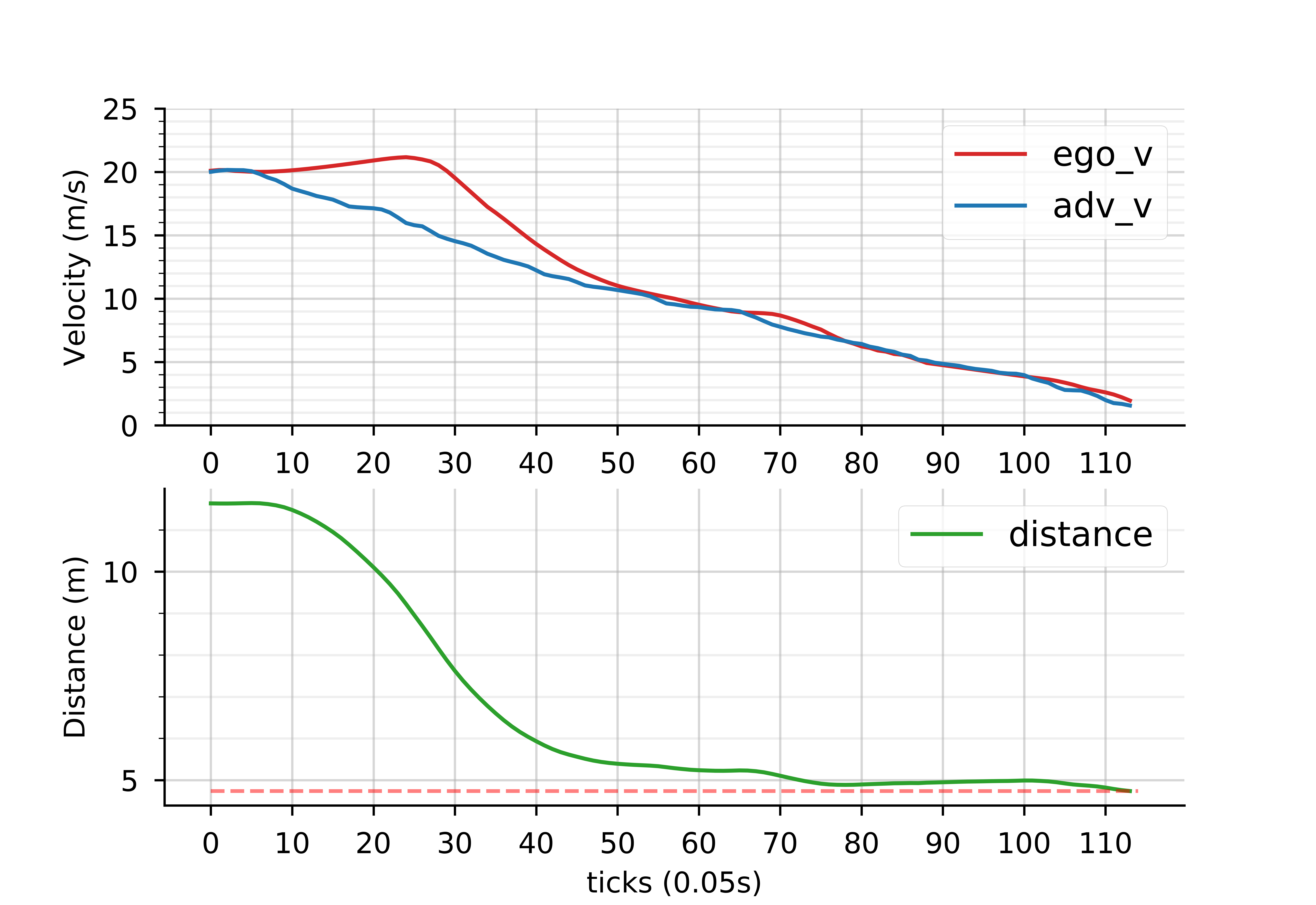
(a)

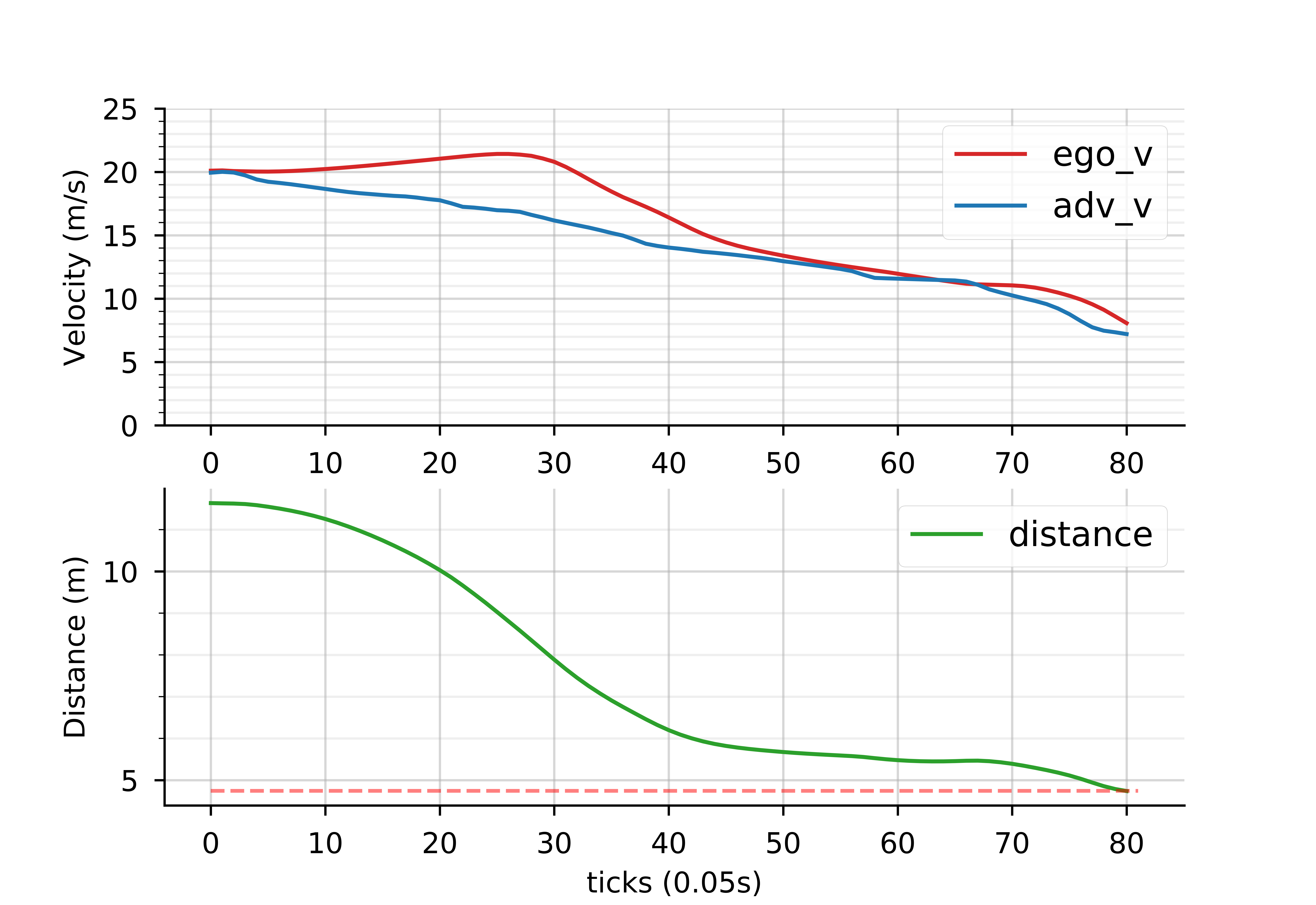
(b)

Figure 2: Traces showing two different ado policies that are able to induce a collision in the ego agent.

Adaptive Cruise Control. In this experiment, two vehicles are driving in a single lane on a highway. The lead vehicle is the ado. The follower vehicle avoids colliding into the leader using an adaptive cruise controller (ACC). The purpose of adversarial testing is to find robust ado policies that cause the ACC system to collide with the ado. The ACC controller modulates the throttle ($\alpha$) by observing the distance ($d$) to the lead vehicle and attempting to maintain a minimum safe following distance $d_{\mathrm{safe}}$. The ACC controller is a Proportional-Derivative (PD) controller with saturation. The PD term $u$ is equal to $K_{p}(d-d_{\mathrm{safe}})+K_{d}(v_{\mathsf{ado}}-v_{\mathsf{ego}})$, and the controller action $\alpha$ is defined as $\alpha_{\max}$ if $u>\alpha_{\max}$, $\alpha_{\min}$ if $u<\alpha_{\min}$, and $u$ otherwise. The ego specification is given in Eq. (LABEL:eq:accegospec). Here, $T$ is the maximum duration of a simulation episode and $d_{\mathrm{safe}}$ is the minimum safe following distance. The ado should cause the ego to violate its spec in less than $T$ seconds. The ado constraint specifies that it should not exceed the speed limit $v_{\lim}$ and that it should maintain a minimum speed $v_{\min}$. For our experiment, we choose $v_{\min}=0.1$, and $d_{\mathrm{safe}}=4.7$m. The distance $d$ is computed between the two front bumpers. This represents a car length of $4.54m$, plus a small safety margin. The state of the ado agent is the tuple $d,v_{\mathsf{ego}},v_{\mathsf{ado}}$. At each time step, the ado agent chooses an acceleration from a discretized space which contains $3$ possible actions. In this experiment, we explore two different RL algorithms: q-learning and a DQN algorithm with replay buffers [29]. The average runtime using the DQN (1.93 hours) is less than that using a Q-table (4.83 hours) and gives comparable success rates: 54.8% for the DQN agent vs. 55.79% for the agent using Q-tables. The average time to run a single episode is between 29 and 30 seconds. Fig. 2 shows 2 episodes from the same initial position for the ego and ado vehicles where the ado is able to induce a collision by the ego.

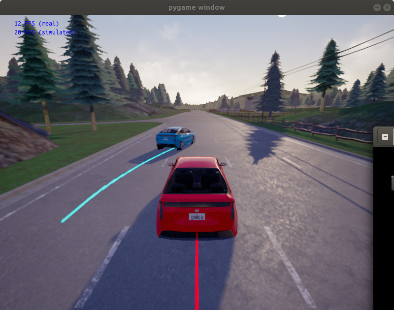
(a) Adversarial vehicle changes lane far away from the ego vehicle.

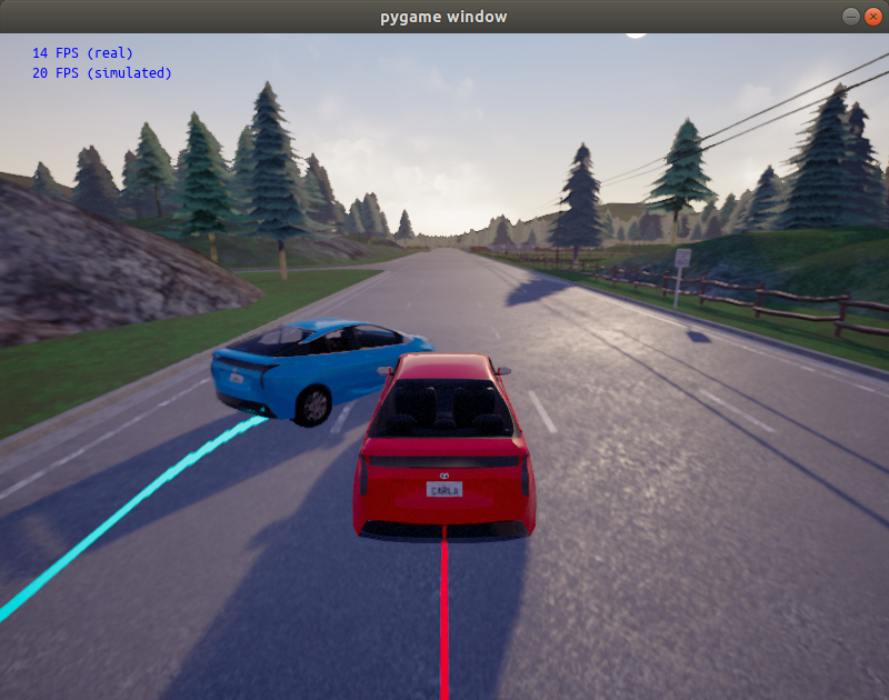
(b) The adversarial vehicle changes lane aggressively and hits the ego vehicle, violating traffic rules.

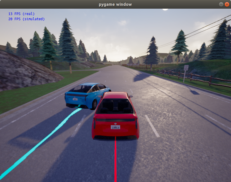
(c) Adversary changes lane and induces a crash without braking the traffic rules

Figure 3: Ado behaviors across episodes in the lane change maneuvers case study.

Lane Change Maneuvers. Here, 2 vehicles are driving on a two-lane highway; the ego controlled by a switching controller that alternates between cruising and avoiding a collision by applying a “hard” brake. The ego controller predicts future ado positions based on the current state using a look-ahead distance $d_{\mathrm{lka}}=d_{\mathrm{lat}}-v_{\mathsf{ado},\mathrm{lat}}t_{\mathrm{lka}}$, where $d_{\mathrm{lat}}$ is the lateral distance between the vehicles, $v_{\mathsf{ado},\mathrm{lat}}$ is the ado’s lateral velocity and $t_{\mathrm{lka}}$ is a fixed look-ahead time. Based on $d_{\mathrm{lka}}$, it switches between two control policies: if $d_{\mathrm{lka}}>d_{\mathrm{safe}}$, then it continues to cruise, but if $d_{\mathrm{lka}}\leq d_{\mathrm{safe}}$, it applies brakes. The ado is in the left lane and attempts to merge to the right in a way that causes the ego to collide with it. We add a constraint to ensure that the ado should always be longitudinally in front of the ego car when it tries to merge as specified in Eq. (LABEL:eq:lcadorule); here $d_{\mathrm{long}}$ is the longitudinal distance between the cars. Without this constraint, the ado can always induce a sideways-crash. The ego spec is given in Eq. (LABEL:eq:lcegospec). Here, $d_{2}=\sqrt{d_{\mathrm{long}}^{2}+d_{\mathrm{lat}}^{2}}$ is the Euclidean distance between the two cars.

In the course of training, we observe that the behavior of the ado agent improves with time. Training for 106 episodes requires 2.53 hours and gives us a success rate of $71\%$, i.e. $71\%$ of the episodes lead to a collision induced in the ego. With 206 episodes, the success rate improves to $72.35\%$ but requires 4.71 hours of runtime. After 371 episodes, the rate improves to $75.76\%$ after 9.44 hours. This experiment demonstrates that even under a small time budget, the constrained RL algorithm can achieve a high amount of success.

Generalizability. In both case studies, we observed generalizability of the ado policy to different initial conditions. In the ACC case study, we found several initial states within $\delta=6.5\times 10^{-6}$ that were also counterexample states. Overall the states have smaller values as the episode lengths are longer and the $\gamma^{T}$ term causes values to be small. We observed that for the failing initial state $(v_{\mathsf{ego}}\mapsto 12,v_{\mathsf{ado}}\mapsto 12,d\mapsto 15)$, we found failing initial states with values of both $v_{\mathsf{ado}}$ and $d$ that were both smaller and larger than those in the original initial state. However, some failing initial states did not have states with nearby values that were violating. This can be attributed to the fact that the RL algorithm may not have converged to a value close to optimal. For the second case study, we found that the failing initial condition $(v_{\mathsf{ego}}\mapsto 12,v_{\mathsf{ado}}\mapsto 12,d_{2}\mapsto 16)$ has several nearby failing initial states with a small value of $\delta$ that were not previously encountered during training.

VI Related Work and Conclusions

Adaptive Stress Testing. The work of [9, 8] is closely related to our work. In this work, the authors also use deep RL (and related Monte Carlo Tree search) algorithms to seek behaviors of the vehicle under test that are failure scenarios. There a few key differences in our approach. In [9], reward functions (that encode failure scenarios) are hand-crafted and require manual insight to make sure that the RL algorithms converge to behaviors that are failure scenarios. Furthermore, the constraints on the adversarial environment are also explicitly specified. The approach in[8] uses a subset of RSS (Responsibility-Sensitive Safety) rules that are used to augment hand-crafted rewards to encode failure scenarios by the ego and responsible behavior by other agents in a scenario. In specifying STL constraints, we remove the step of manually crafting rewards.

Falsification. There is extensive related work in falsification of cyber-physical system. Most falsification techniques use fixed finitary parameterization of system input signals to define a finite-dimensional search space, and use global optimizers to search for parameter values that lead to violation of the system specification. A detailed survey of falsification techniques can be found in [6]. A control-theoretic view of falsification tools is that they learn open-loop adversarial policies for falsifying a given ego model while our approach focuses on closed-loop policies.

Falsification using RL. Also close to our work are recent approaches to use RL [4] and deep RL [3] for falsification. The key focus in [4] is on solving the problem of automatically scaling quantitative semantics for predicates and effective handling of Boolean connectives in an STL formula. The work in [3] focuses on a smooth approximation of the robustness of STL and thoroughly benchmarks the use of different deep RL solvers for falsification.

Comparison. Compared to previous approaches, the focus of our paper is on reusability of dynamically constrained adversarial agents trained using RL techniques. We identify conditions under which a trained adversarial policy is applicable to a system with a different initial condition or different dynamics with no retraining. This can be of immense value in an incremental design and verification approach. The other main contribution is that instead of using a monolithic falsifier, our technique packs multiple, dynamically constrained falsification engines as separate agents; dynamic constraints allow us to specify hierarchical traffic rules. Furthermore, previous approaches for falsification do not consider dynamic constraints on the environment at all – constraints are limited to simple bounds on the parameter space. Finally, in our approach, both specifications and constraints are combined into a single reward function which can then utilize off-the-shelf deep RL algorithms. In comparison to [4, 3, 30], our encoding of STL formulas into reward functions is simplistic as it is not the main focus of this paper; we defer extensions that consider nuanced encoding of STL constraints to future work.

Conclusions. Our work addresses the problem of automatically performing constrained stress-testing of cyberphysical systems. We use STL to specify the target against which we are testing and constraints that specify reasonableness of the testing regime. We are using STL as a lightweight, high-level programming language to loosely specify the desired behaviors of a test scenario, and leveraging powerful RL algorithms to determine how to execute those behaviors. The learned adversarial policies are reactive, as opposed to testing schemes that rely on merely replaying pre-recorded behaviors, and under limited conditions can even provide valuable testing capability to modified versions of the system.

Appendix

Tool Pipeline. The tool pipeline is illustrated in Figure 4. The ego agent interacts with several ado agents as part of a simulation. The ados are able to observe the state of the ego as well as of the other ado agents, and they may update their policies.

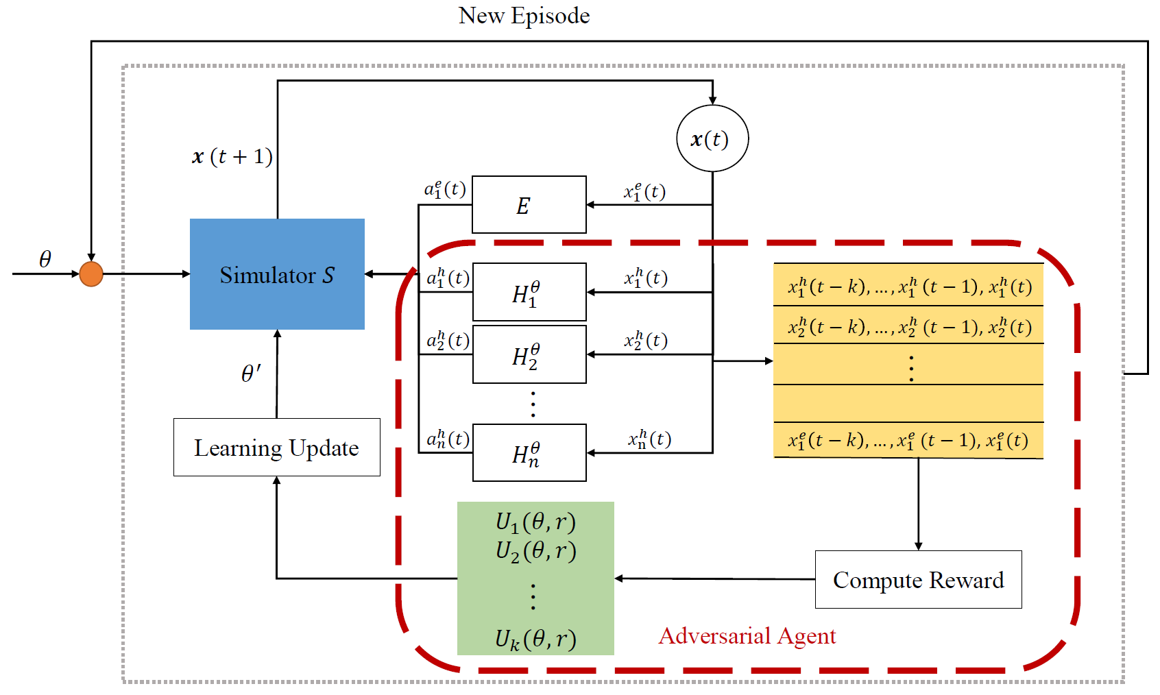
Figure 4: The ego agent $E$ is embedded in a simulation with a collection of adversarial agents $H_{i}^{\theta}$, which learn (possibly from a bank of past experience) to stress-test the ego by a particular reward function as derived from the rulebook constraints for the adversary and the ego specification.

Lemma 3 (Soundness of the reward function).

Consider two traces, $s_{1}$ and $s_{2}$. Suppose that the highest priority constraint violated by $s_{1}$ is $c_{1}$ and the highest priority constraint violated by $s_{2}$ is $c_{2}$. Suppose $c_{1}$ has lower priority than $c_{2}$. Then, the reward for trajectory 1 will be higher than the reward for trajectory 2, i.e. $R(s_{1})>R(s_{2})$.

Proof.

Let $n_{1}$ be the number of rules with priority less than or equal to $c_{1}$. Similarly, let $n_{2}$ the number of rules with priority less than or equal to $c_{2}$. Then, $R(s_{1})=-n_{1}\rho_{min}$ and $R(s_{2})=-n_{2}\rho_{min}$. Since $n_{2}>n_{1}$ by the assumptions of the lemma, the result follows. ∎

Yellow Light. In this experiment, the ego vehicle is approaching a yellow traffic light led by an ado vehicle. Let the signed distance of the ego, ado from the light be respectively $d_{\ell,\mathsf{ego}}$, $d_{\ell,\mathsf{ado}}$, and Boolean variables $\ell_{Y}$ and $\ell_{R}$ be true if the light is respectively yellow and red. We use the convention that $d_{\ell,\mathsf{ego}}>-\delta$ if the ego vehicle is approaching the light and $d_{\ell,\mathsf{ego}}<-\delta$ if it has passed the light (resp. for ado). By traffic rules, a vehicle is expected to stop $\delta$ meters away from the traffic light (e.g. $\delta$ could be the width of the intersection being controlled by the light), I.e. the vehicle should stop at $0$. Thus, if $d_{\ell,\mathsf{ego}}\in[-\delta,0]$ when the light turns red, it has run the red light. This ego specification is shown in Eq. (LABEL:eq:ylegospec). The traffic light is modeled as a non-adversarial agent, it merely changes its state based on a pre-determined schedule. The goal of the ado vehicle is to make the ego vehicle run the red light. The rulebook constraints on the ado vehicle are that it may not drive backwards and it may not run the red light (shown in Eqs. (LABEL:eq:yladoruleone),(LABEL:eq:yladoruletwo) resp.). The state of the ado agent includes the speed of both vehicles, and relative distance between the vehicles. At the start of an episode, $d_{\ell,\mathsf{ado}}=30$, and $\ell_{Y}$ is true, and $\ell_{R}$ becomes true after $\tau=2$ seconds.

The ego controller is a switched mode controller that either uses an ACC controller or applies the maximum available deceleration $a_{\mathsf{ego},\max}$. At time $t<\tau$, let $d(t)$ denote the distance required for the ego vehicle to come to a stop before the light turns red by applying $a_{\mathsf{ego},\max}$. We can calculate $d(t)$ as $v_{\mathsf{ego}}\cdot(\tau-t)+0.5\cdot a_{\mathsf{ego},\max}\cdot(\tau-t)^{2}$. Then, at time $t$, the ego controller chooses to cruise if $d(t)+\delta<d_{\ell,\mathsf{ego}}$, and brakes otherwise.

Figure 5 shows that the ego vehicle maintains an appropriate distance to the lead car, but that it starts decelerating too late and is thus caught in the intersection when light turns red. The adversarial vehicle successfully clears the intersection while the light is still yellow, consistent with its rulebook constraints. The ado agent we train uses the DQN RL algorithm. After 162 episodes of training, approximately 60% of its episodes find a violation of the ego specification with a runtime of 1.88 hours. After 247 episodes, the success rate increases to 64% with a runtime of 2.59 hours. This case study demonstrates that our adversarial testing procedure succeeds even in the presence of multiple ado rules and an interesting ego specification.

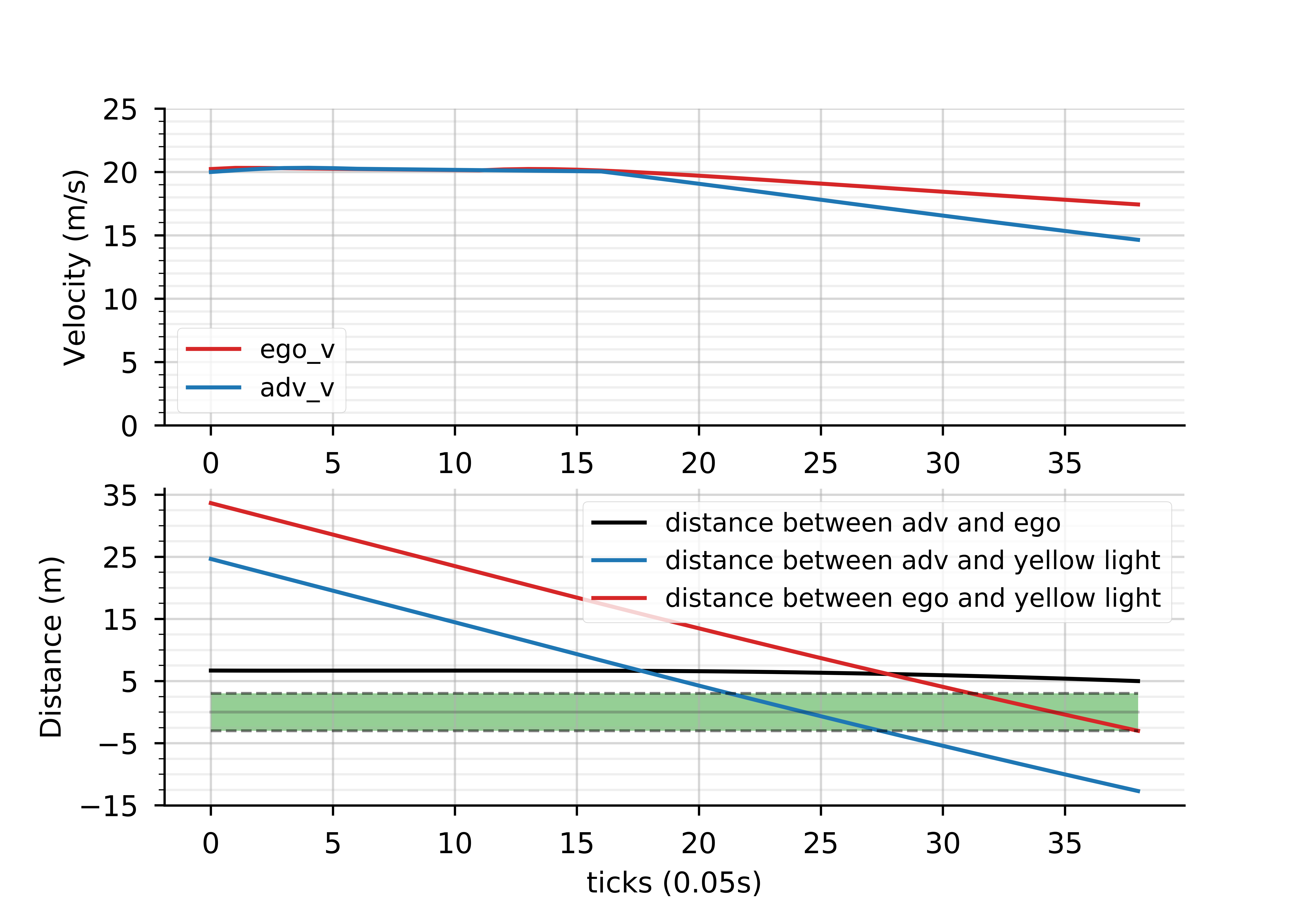
Figure 5: Yellow light case study. The green region represents the region in which the ego vehicle will run the yellow light. The adversary learns to drive the ego car into the target region.

Case Study	Description	STL Formula
Yellow	Ego: Don’t run red light	$\displaystyle\neg\mathbf{F}_{[0,T]}(\ell_{R}\wedge d_{\ell,\mathsf{ego}}\in[-\delta,0])$	(20)q:ylegospec
Light	Ado: Speed Limits	$\displaystyle\mathbf{G}_{[0,T]}(v_{\mathsf{ado}}<v_{\lim})$	(21)q:yladoruleone
	Ado: Don’t run red light	$\displaystyle\neg\mathbf{F}_{[0,T]}(\ell_{R}\wedge d_{\ell,\mathsf{ado}}\in[-\delta,0])$	(22)q:yladoruletwo

TABLE III: Ego Specifications and Ado Rules for case studies

References

- [1] Y. S. R. Annapureddy, C. Liu, G. E. Fainekos, and S. Sankaranarayanan, “S-TaLiRo: A Tool for Temporal Logic Falsification for Hybrid Systems,” in Proc. of Tools and Algorithms for the Construction and Analysis of Systems, 2011, pp. 254–257.
- [2] A. Donzé, “Breach, a toolbox for verification and parameter synthesis of hybrid systems,” in International Conference on Computer Aided Verification. Springer, 2010, pp. 167–170.
- [3] T. Akazaki, S. Liu, Y. Yamagata, Y. Duan, and J. Hao, “Falsification of cyber-physical systems using deep reinforcement learning,” in International Symposium on Formal Methods. Springer, 2018, pp. 456–465.
- [4] Z. Zhang, I. Hasuo, and P. Arcaini, “Multi-armed bandits for boolean connectives in hybrid system falsification,” in Computer Aided Verification, I. Dillig and S. Tasiran, Eds. Cham: Springer International Publishing, 2019, pp. 401–420.
- [5] Z. Zhang, P. Arcaini, and I. Hasuo, “Hybrid System Falsification Under (In)equality Constraints via Search Space Transformation,” IEEE Transactions on Computer-Aided Design of Integrated Circuits and Systems, 2020.
- [6] J. V. Deshmukh and S. Sankaranarayanan, “Formal techniques for verification and testing of cyber-physical systems,” in Design Automation of Cyber-Physical Systems. Springer, 2019, pp. 69–105.
- [7] S. Ali, L. C. Briand, H. Hemmati, and R. K. Panesar-Walawege, “A systematic review of the application and empirical investigation of search-based test case generation,” IEEE Transactions on Software Engineering, vol. 36, no. 6, pp. 742–762, 2009.
- [8] A. Corso, P. Du, K. Driggs-Campbell, and M. J. Kochenderfer, “Adaptive stress testing with reward augmentation for autonomous vehicle validatio,” in 2019 IEEE Intelligent Transportation Systems Conference (ITSC). IEEE, 2019, pp. 163–168.
- [9] M. Koren, S. Alsaif, R. Lee, and M. J. Kochenderfer, “Adaptive stress testing for autonomous vehicles,” in 2018 IEEE Intelligent Vehicles Symposium (IV). IEEE, 2018, pp. 1–7.
- [10] D. Amodei, C. Olah, J. Steinhardt, P. Christiano, J. Schulman, and D. Mané, “Concrete Problems in AI Safety,” Jun. 2016. [Online]. Available: http://arxiv.org/abs/1606.06565
- [11] O. Maler and D. Nickovic, “Monitoring temporal properties of continuous signals,” in FORMATS. Springer, 2004, pp. 152–166.
- [12] G. E. Fainekos and G. J. Pappas, “Robustness of temporal logic specifications for continuous-time signals,” Theoretical Computer Science, 2009.
- [13] O. Maler and D. Nickovic, “Monitoring Temporal Properties of Continuous Signals,” in Formal Techniques, Modelling and Analysis of Timed and Fault-Tolerant Systems, 2004.
- [14] S. Jakšić, E. Bartocci, R. Grosu, T. Nguyen, and D. Ničković, “Quantitative monitoring of STL with edit distance,” Formal Methods in System Design, vol. 53, no. 1, pp. 83–112, Aug. 2018.
- [15] A. Donzé and O. Maler, “Robust Satisfaction of Temporal Logic over Real-Valued Signals,” in Formal Modeling and Analysis of Timed Systems. Berlin, Heidelberg: Springer Berlin Heidelberg, 2010, vol. 6246, pp. 92–106.
- [16] R. Bloem, K. Chatterjee, and B. Jobstmann, “Graph games and reactive synthesis,” in Handbook of Model Checking. Springer, 2018, pp. 921–962.
- [17] R. Dimitrova and R. Majumdar, “Deductive control synthesis for alternating-time logics,” in 2014 International Conference on Embedded Software (EMSOFT). IEEE, 2014, pp. 1–10.
- [18] J. Liu, N. Ozay, U. Topcu, and R. M. Murray, “Synthesis of reactive switching protocols from temporal logic specifications,” IEEE Transactions on Automatic Control, vol. 58, no. 7, pp. 1771–1785, 2013.
- [19] V. Raman, A. Donzé, D. Sadigh, R. M. Murray, and S. A. Seshia, “Reactive synthesis from signal temporal logic specifications,” in Proceedings of the 18th international conference on hybrid systems: Computation and control, 2015, pp. 239–248.
- [20] S. Ghosh, D. Sadigh, P. Nuzzo, V. Raman, A. Donzé, A. L. Sangiovanni-Vincentelli, S. S. Sastry, and S. A. Seshia, “Diagnosis and repair for synthesis from signal temporal logic specifications,” in Proceedings of the 19th International Conference on Hybrid Systems: Computation and Control, 2016, pp. 31–40.
- [21] R. S. Sutton and A. G. Barto, Reinforcement learning: an introduction, second edition ed., ser. Adaptive computation and machine learning series. Cambridge, MA: The MIT Press, 2018.
- [22] V. Mnih, K. Kavukcuoglu, D. Silver, A. Graves, I. Antonoglou, D. Wierstra, and M. Riedmiller, “Playing Atari with Deep Reinforcement Learning,” in NIPS, 2013, arXiv: 1312.5602. [Online]. Available: http://arxiv.org/abs/1312.5602
- [23] J. Schulman, F. Wolski, P. Dhariwal, A. Radford, and O. Klimov, “Proximal policy optimization algorithms,” arXiv preprint arXiv:1707.06347, 2017.
- [24] A. Censi, K. Slutsky, T. Wongpiromsarn, D. Yershov, S. Pendleton, J. Fu, and E. Frazzoli, “Liability, Ethics, and Culture-Aware Behavior Specification using Rulebooks,” in ICRA, 2019.
- [25] N. Ferns, P. Panangaden, and D. Precup, “Bisimulation metrics for continuous Markov decision processes,” SIAM Journal on Computing, vol. 40, no. 6, pp. 1662–1714, 2011.
- [26] A. Girard and G. J. Pappas, “Approximate Bisimulation: A Bridge Between Computer Science and Control Theory,” European Journal of Control, vol. 17, no. 5, pp. 568–578, Jan. 2011.
- [27] A. Dosovitskiy, G. Ros, F. Codevilla, A. Lopez, and V. Koltun, “CARLA: An open urban driving simulator,” in Proceedings of the 1st Annual Conference on Robot Learning, 2017, pp. 1–16.
- [28] A. Paszke, S. Gross, F. Massa, A. Lerer, J. Bradbury, G. Chanan, T. Killeen, Z. Lin, N. Gimelshein, L. Antiga, A. Desmaison, A. Kopf, E. Yang, Z. DeVito, M. Raison, A. Tejani, S. Chilamkurthy, B. Steiner, L. Fang, J. Bai, and S. Chintala, “Pytorch: An imperative style, high-performance deep learning library,” in Advances in Neural Information Processing Systems 32, H. Wallach, H. Larochelle, A. Beygelzimer, F. d’Alché Buc, E. Fox, and R. Garnett, Eds. Curran Associates, Inc., 2019, pp. 8024–8035.
- [29] V. Mnih, K. Kavukcuoglu, D. Silver, A. Graves, I. Antonoglou, D. Wierstra, and M. A. Riedmiller, “Playing atari with deep reinforcement learning,” ArXiv, vol. abs/1312.5602, 2013.
- [30] K. Leung, N. Aréchiga, and M. Pavone, “Backpropagation for parametric stl,” in 2019 IEEE Intelligent Vehicles Symposium (IV). IEEE, 2019, pp. 185–192.