When does Diversity Help Generalization in Classification Ensembles?

Abstract

Ensembles, as a widely used and effective technique in the machine learning community, succeed within a key element—“diversity.” The relationship between diversity and generalization, unfortunately, is not entirely understood and remains an open research issue. To reveal the effect of diversity on the generalization of classification ensembles, we investigate three issues on diversity, i.e., the measurement of diversity, the relationship between the proposed diversity and the generalization error, and the utilization of this relationship for ensemble pruning. In the diversity measurement, we measure diversity by error decomposition inspired by regression ensembles, which decomposes the error of classification ensembles into accuracy and diversity. Then we formulate the relationship between the measured diversity and ensemble performance through the theorem of margin and generalization and observe that the generalization error is reduced effectively only when the measured diversity is increased in a few specific ranges, while in other ranges larger diversity is less beneficial to increasing the generalization of an ensemble. Besides, we propose two pruning methods based on diversity management to utilize this relationship, which could increase diversity appropriately and shrink the size of the ensemble without much-decreasing performance. Empirical results validate the reasonableness of the proposed relationship between diversity and ensemble generalization error and the effectiveness of the proposed pruning methods.

I Introduction

Ensemble learning has attracted plenty of research attention in the machine learning community thanks to its remarkable potential [1], and it has been widely used in many real-world applications such as object detection, object recognition, object tracking [2, 3, 4, 5], fault diagnosis, malware detection, depression detection [6, 7, 8], and so on [9, 10, 11, 12, 13, 14, 15, 16, 17, 18, 19]. Rather than relying on one single model, an ensemble is a set of learned models that make decisions collectively. It is widely accepted that an ensemble usually generalizes better than one single model [20, 21, 22, 23]. Dietterich [24] stated that an ensemble of classifiers succeeded in better accuracy if and only if its individual members are accurate and diverse. One classifier is accurate if its error rate is better than random guessing on new instances. Two classifiers are diverse if they make different errors in new instances. The diversity of an ensemble usually decreases with the increasing of accuracies of its members [25]. Thus, how to handle the trade-off between accuracy and diversity appropriately is a crucial issue in ensemble learning.

Unfortunately, there is still no consensus in the community on the definition or measurement for diversity, unlike the precise accuracy. Existing ensemble methods create different classifiers implicitly or heuristically by manipulating input data, input features, or output targets. Existing diversity measures are various, yet none of them show superiority over each other [26, 23, 27]. They are generally divided into pairwise and non-pairwise diversity measures [28, 1]. Lots of previous work made an effort to seek the role of diversity in ensemble learning [29, 30, 31, 32]. In regression ensembles, the diversity is defined based on the error decomposition [33], in which the error of regression ensembles is split into the accuracy term and diversity term. The classic Ambiguity Decomposition [33] and Bias-Variance-Covariance decomposition [34] are two commonly used error decomposition schemes. However, both of them are only suitable for regression tasks with the square loss.

Moreover, the relationship between diversity and generalization in the literature remains an open question. Some researchers, such as Kuncheva and Whitaker [28], hold doubts about the usefulness of diversity measures in building classification ensembles in real-life pattern recognition problems. Conversely, some researchers hold the view as well that diversity among the members of a team of classifiers is a crucial issue in classifiers’ combination [35]. They are two inconsistent views, so, weirdly, both of them have some supporting experimental results in some cases. For instance, some empirical results [28] showed less correlation between diversity and generalization error by varying the diversity in the ensemble. Meanwhile, some experiments [31] showed precisely the opposite results. Hence, to clarify this issue, whether or not diversity affects the performance of generalization becomes particularly essential.

Inspired by error decomposition of regression ensembles, we propose a measure of diversity using error decomposition for classification ensembles with the $0/1$ error function firstly, where the error of classification ensembles is split into two terms: accuracy and diversity. Like regression ensembles, the diversity term measures the difference among members of classification ensembles. Secondly, we propose the relationship between the proposed diversity and generalization using the proposed diversity measure based on [36, 37]. By taking bagging and AdaBoost as examples of ensemble methods, experiments are conducted to validate the proposed relationship by varying the diversity in bagging and AdaBoost. Thirdly, we propose an ensemble pruning method named as “Ensemble Pruning based on Diversity (EPBD),” which utilizes the proposed relationship between the proposed diversity and generalization to improve the ensemble’s generalization. To extend EPBD to use other diversity measures, we propose an ensemble pruning framework named as “Ensemble Pruning Framework Utilizing the Trade-off Between Accuracy and Diversity (FTAD)” as well, which utilizes the trade-off between accuracy and diversity. Moreover, empirical results are presented to validate the effectiveness of EPBD and FTAD. The contributions in this paper are three-fold:

• A diversity measure based on error decomposition is proposed to quantify the difference among classification ensemble members, for the benefit of conducting theoretical analyses later.

• The relationship between the proposed diversity and the ensemble generalization error is investigated and analyzed theoretically, which demonstrates that diversity has different impacts on the ensemble generalization in different ranges.

• Two ensemble pruning methods are proposed to select a subset of the original ensemble, while one utilizes the proposed theoretical relationship and the other as an extension of the former utilizes the trade-off between accuracy and diversity.

The rest of this paper is organized as follows. The related work is summarized in Section II. And then, the core investigations are presented in Section III, answering three issues about diversity: (1) the measurement of diversity and its corresponding properties in Section III-A and III-B; (2) the relationship between the proposed diversity and generalization error of ensembles in Section III-C; (3) the utilization of this relationship about diversity in Section III-D and III-E. Finally, the empirical results are presented in Section IV, followed by the conclusion in Section V.

II Related Work

Diversity is considered intuitively as the difference among individual members in an ensemble, with several alternative names such as dependence, orthogonality, or complementarity [28, 1]. In this section, we introduce existing methods to generate diverse individual classifiers in ensemble learning. Then we describe existing methods to measure diversity in ensemble learning. Finally, we summarize some research about the crucial role diversity plays in ensemble learning.

II-A Generating Diverse Individual Classifiers for Ensembles

Most ensemble methods attempt to generate diverse classifiers implicitly or heuristically by manipulating the input data or features, while few of them manipulate output targets [24, 31]. For example, bagging [38] and Boosting (including many variants) [39, 40, 41] manipulate input data to promote diversity by choosing different subsets of the training data during training; Random forest [42] manipulates subsets of input data or features to create diversity and gives competitive results; Rotation forest [43] applies principal component analysis (PCA) on each subset as an improved method. Moreover, neural network (NN) ensembles also create diversity using different initial weights, different architectures of the networks, or different learning algorithms. However, the diversity generated by these methods is not precise and could not tell how much diversity in their generating process or whether diversity in ensembles should be increased or not for the specific ensemble.

II-B Diversity Measurements in Ensembles

Diversity is usually measured based on the classification results of individual members in an ensemble [44, 35, 30, 26, 45, 46]. Existing diversity measures are generally divided into pairwise and non-pairwise diversity measures [28, 1]. Based on the coincident errors between pairs of individual classifiers, pairwise diversity represents the behavior if both of them predict an instance identically or disagree with each other. In this case, the overall diversity is the average of all possible pairs [23]. Pairwise diversity includes $Q$-statistic [47], $\kappa$-statistic [48], disagreement measure [49, 50], correlation coefficient [51], double-fault [52], and the hamming distance (HD) measure [46]. In contrast, non-pairwise diversity directly measures a set of classifiers using the variance, entropy, or the proportion of individual classifiers that fail on randomly chosen instances [23]. It includes interrater agreement [53], Kohavi-Wolpert variance [54], the entropy of the votes [55, 56], the difficulty index [57, 28], the generalized diversity [58], and the coincident failure diversity [58]. Apart from those, two other measures exist and do not fall into the categories above. One is the correlation penalty function, proposed by Liu and Yao [59] in their negative correlation learning (NCL) [60]. It measures the diversity of each member against the entire ensemble. The other is ambiguity, which measures the average offset of each member against the entire ensemble output [61]. Due to the examined difference or similarity, the ranges of diversity vary between different diversity measures [1]. Moreover, comparing those existing diversity measures is difficult regarding the appropriateness and superiority across them [23]. The performance of a diversity measure might depend on the context of data and the use of diversity [27].

II-C The Role that Diversity Plays

Although the crucial role of diversity has been widely accepted, few researchers could tell how diversity works exactly in ensemble methods. In the last decade or so, Brown [29] claimed that from an information-theoretic perspective, diversity within an ensemble did exist on numerous levels of interaction between the classifiers. This work inspired Zhou and Li [30] to propose that the mutual information should be maximized to minimize the prediction error of an ensemble from the view of multi-information. Subsequently, Yu et al. [31] claimed that the diversity among individual learners in a pairwise manner, used in their diversity regularized machine (DRM), could reduce the hypothesis space complexity, which implied that controlling diversity played the role of regularization in ensemble methods. Recently, Jiang et al. [32] extended the classic Ambiguity Decomposition from regression problems to classification problems and proved several fundamental properties of the Ambiguity term.

II-D Ensemble Pruning

Ensemble pruning, named as ensemble selection or ensemble thinning as well, is proposed to mitigate the shortcoming of ensemble methods that usually require huge memory and processing time regarding the number of individual learners in the ensemble [62, 63, 64, 65, 66, 67, 68]. It is possible to improve the ensemble generalization performance with a smaller size using ensemble pruning [69, 70]. Selecting the sub-ensembles with the best generalization is quite challenging with exponential computational complexity [35, 71]. Existing ensemble pruning methods could be categorized basically into three general families: ranking-based, clustering-based, and optimization-based. Ranking-based pruning methods sort the learners in the ensemble based on different evaluation function and select the top few of them [72, 73, 74], with a low searching complexity yet theoretical unsoundness [75]; Clustering-based pruning methods detect groups of learners making similar predictions and prune each group separately [76, 77]; Optimization-based pruning methods utilize different objectives to optimize and find the expected subset with satisfactory generalization performance [78, 79, 80, 81, 82, 83], requiring an optimization searching algorithm to avoid exhaustive search complexity [75]. Another partition divides ensemble pruning methods into static and dynamic pruning techniques [84]. Static pruning techniques focus on identify a small sub-ensemble with good generalization performance, accompanied by expensive computation [85, 86, 87, 35, 88, 25]; Dynamic pruning techniques [89, 90, 91] determine the number of individual classifiers that need to be queried dynamically for each test instance, reducing the time cost yet not reducing the ensemble’s storage requirements [89, 92, 93, 94, 95]. Besides, Jiang et al. [96] presented a Bayesian framework for ensemble pruning which generated the optimal size of the pruned ensemble first and selected the optimal pruned ensemble accordingly; Krawczyk and Wozniak [97] proposed to do ensemble pruning tasks considering the combination rule training simultaneously.

III Methodology

In this section, we formally study the measure of diversity using error decomposition of classification ensembles and derive proper theoretical analyses from quantifying and characterizing the relationship between the proposed diversity and generalization performance of the entire ensemble. Based on the results of the analyses, two ensemble pruning methods are proposed to construct a pruned sub-ensemble effectively.

We first introduce the necessary notations used in this paper. Let vectors be denoted by bold lowercase letters (e.g., $\mathbf{x}=(x_{1},...,x_{k})$) as an instance with $k$-tuples of real numbers describing features, and scalars denoted by italic lowercase letters (e.g., $y$) as labels. Random variables, (vector) spaces, and subsets of these vector spaces are denoted by sans serif uppercase letters (e.g., $\mathsf{X}$), calligraphic uppercase letters (e.g., $\mathcal{X}$), and roman uppercase letters (e.g., $W$), respectively. Sets of vectors are denoted by roman uppercase letters (e.g., $S$) consisting of some instances with their corresponding labels; individual classifiers/learners are denoted by functions (e.g., $f(\cdot)$) as the output results of one classifier. The symbols $\mathbf{P},\,\mathbf{E}\,,$  $\mathbb{I}$ ,  $\mathbb{R}$ ,  and $\mathbb{Z}^{+}$ denote the probability measure, the expectation of a random variable, the indicator function, the real space, and the positive integer space, respectively. The notation $[n]$ represents $\{1,...,n\}$ for clarity. The notation $(\mathbf{x},y)\in S$ is formally defined by $(\mathbf{x},y)\in S\Leftrightarrow\exists\,i\in[|S|]:(\mathbf{x}_{i},y_{i})=(\mathbf{x},y)$ for clarity.

Figure 1: Illustration for the proposed methodology. (a) Illustration for the error decomposition for classification ensembles (in Theorem 1). (b) Illustration of Lemma 1 [36, 37]. (c) Illustration for the relationship between the proposed diversity and ensemble performance motivated by [36, 37]. Herbrich and Graepel [36, 37] proposed the relationship between margin and generalization (in Lemma 1). Besides, the proposed diversity in Eq. (11) is related to the margin. In this case, we could propose the relationship between the proposed diversity and ensemble performance (in Theorem 2). Note that the arrow from A to B means that B is related to A, where arrows in solid lines represent direct relations and that in the dotted line represents the indirect relation.

III-A Measuring Diversity in Classification Ensembles using Error Decomposition

The analysis is built in the PAC (probably approximately correct) framework [98] that one learning task $\mathcal{D}$ corresponds to a probability distribution over the input-output space $\mathcal{X}\times\mathcal{Y}$. An instance from $\mathcal{D}$ is represented as $(\mathbf{x},y)\,,$ where $\mathbf{x}\in\mathbb{R}^{k}$ is a vector representing features and $y$ is a scalar as a label. Suppose this classification task is to use an ensemble that comprises several individual classifiers to approximate a function $f_{true}:\mathcal{X}\mapsto\mathcal{Y}\,,$ and $F=\{f_{1},...,f_{|F|}\}$ denotes the set of these individual classifiers. The predictions of the individual classifiers are combined by weighted voting, that is, the output of an ensemble is defined as:

$$\small f_{ens}(\mathbf{x})=\mathop{\rm{sgn}}\Bigg{(}\sum_{i\in[|F|]}w_{i}\cdot f_{i}(\mathbf{x})\Bigg{)}\,,$$ (1)

where $w_{i}$ is the weight coefficient corresponding to the individual classifier $f_{i}$ , satisfying that $\sum_{i\in[|F|]}w_{i}=1,\,\forall w_{i}\geqslant 0$. And $\sum_{i\in[|F|]}w_{i}f_{i}(\mathbf{x})=0$ indicates a tie in the combination.

In this work, we focus on binary classification problems that mean $\mathcal{Y}=\{-1,+1\}$, but these theoretical results could be extended to multi-classification problems (a short example is given in the appendix and more research is left for our future work). Assume that there is a training set $S$ with several instances $(\mathbf{x},y)$. For one single arbitrary instance $\mathbf{x}\in S\,,\,y$ denotes the target output of this instance, and $f(\mathbf{x})$ is the actual output of the individual classifier $f\in F\,.$ Notice that $y$ and $f(\mathbf{x})$ satisfy that $y,f(\mathbf{x})\in\mathcal{Y}\,.$ If the actual output of the individual classifier is correct according to the target output, obviously $f(\mathbf{x})\cdot y=+1\,,$ otherwise $f(\mathbf{x})\cdot y=-1\,,$ where this term is defined as the margin of this classifier on the instance,

$$\small\mathop{\rm{margin}}(f,\mathbf{x})=f(\mathbf{x})\cdot y\,.$$ (2)

As the original error decomposition in regression [33, 99, 100] uses the square loss as the loss function that is not suitable for classification, we employ the $0/1$ error function to adopt the idea of error decomposition for regression ensembles. For classification problems, the error function of a classifier $f$ at one single arbitrary instance $\mathbf{x}$ is defined as

$$\small\begin{split}\mathop{\rm{Err}}(f,\mathbf{x})=\begin{cases}1\,,&\text{ if }f(\mathbf{x})y=-1\,;\\ 0.5\,,&\text{ if }f(\mathbf{x})y=0\,;\\ 0\,,&\text{ if }f(\mathbf{x})y=1\,,\end{cases}\end{split}$$ (3)

which is also the discretization of hinge loss function and holds that $\mathop{\rm{Err}}(f,\mathbf{x})=-\frac{1}{2}(f(\mathbf{x})y-1)$. Therefore, inspired by the work of [99, 32], we present the following error decomposition for classification ensembles.

Theorem 1 (Error decomposition for classification ensembles).

Assume that we are dealing with binary classification problems. Individual classifiers in an ensemble $F=\{f_{1},...,f_{|F|}\}$ have been trained and are combined by weighted voting $f_{ens}(\mathbf{x})=\mathop{\rm{sgn}}\big{(}\sum_{i\in[|F|]}w_{i}f_{i}(\mathbf{x})\big{)}$ with $\sum_{i\in[|F|]}w_{i}=1,\,\forall w_{i}\geqslant 0$ . Then for the $0/1$ error function, the loss function of the ensemble can be decomposed into

$$\mathop{\rm{Err}}(f_{ens},\mathbf{x})= \sum_{i\in[|F|]}w_{i}\cdot\mathop{\rm{Err}}(f_{i},\mathbf{x})$$

$$- \frac{1}{2}\Bigg{(}\mathop{\rm{margin}}(f_{ens},\mathbf{x})-\sum_{i\in[|F|]}w_{i}\cdot\mathop{\rm{margin}}(f_{i},\mathbf{x})\Bigg{)}\,.$$ (4)

Computing the expectation in the data set $S$ yields decomposition of the generalization error as follows,

$$\small\bar{G}=\bar{A}-\bar{D}\,,$$ (5)

where

$$\bar{G}= \mathbf{E}_{(\mathbf{x},y)\in S}(\mathop{\rm{Err}}(f_{ens},\mathbf{x}))\,,$$ (6a)

$$\bar{A}= \sum_{i\in[|F|]}w_{i}\cdot\mathbf{E}_{(\mathbf{x},y)\in S}(\mathop{\rm{Err}}(f_{i},\mathbf{x}))\,,$$ (6b)

$$\bar{D}= \frac{1}{2}\mathbf{E}_{(\mathbf{x},y)\in S}(\mathop{\rm{margin}}(f_{ens},\mathbf{x}))$$

$$- \frac{1}{2}\sum_{i\in[|F|]}w_{i}\cdot\mathbf{E}_{(\mathbf{x},y)\in S}(\mathop{\rm{margin}}(f_{i},\mathbf{x}))\,.$$ (6c)

Proof.

For one single arbitrary instance $\mathbf{x}$ , the error of an ensemble is defined as

$$\small\mathop{\rm{Err}}(f_{ens},\mathbf{x})=-\frac{1}{2}\Bigg{(}\mathop{\rm{sgn}}\Bigg{(}\sum_{i\in[|F|]}w_{i}f_{i}(\mathbf{x})\Bigg{)}y-1\Bigg{)}\,.$$ (7)

Inspired by the error decomposition of regression ensembles, the difference between ensemble error and the average error of individual classifiers is

$$\mathop{\rm{Err}}(f_{ens},\mathbf{x})-\sum_{i\in[|F|]}w_{i}\cdot\mathop{\rm{Err}}(f_{i},\mathbf{x})$$

$$= \sum_{i\in[|F|]}w_{i}\cdot\Big{(}\mathop{\rm{Err}}(f_{ens},\mathbf{x})-\mathop{\rm{Err}}(f_{i},\mathbf{x})\Big{)}$$

$$= -\frac{y}{2}\sum_{i\in[|F|]}w_{i}\cdot\big{(}f_{ens}(\mathbf{x})-f_{i}(\mathbf{x})\big{)}\,,$$ (8)

and the error decomposition could be rewritten as

$$\mathop{\rm{Err}}(f_{ens},\mathbf{x})= \sum_{i\in[|F|]}w_{i}\cdot\mathop{\rm{Err}}(f_{i},\mathbf{x})$$

$$- \frac{1}{2}\sum_{i\in[|F|]}w_{i}\big{(}f_{ens}(\mathbf{x})-f_{i}(\mathbf{x})\big{)}y\,.$$ (9)

The first term, $\sum_{i\in[|F|]}w_{i}\cdot\mathop{\rm{Err}}(f_{i},\mathbf{x})$ , is the weighted average loss of the individuals. The second term is defined as the diversity term which measures the difference between $f_{ens}(\mathbf{x})$ and individual classifiers, and it could be rewritten as

$$\frac{1}{2}\sum_{i\in[|F|]}w_{i}\big{(}f_{ens}(\mathbf{x})-f_{i}(\mathbf{x})\big{)}y$$

$$= \frac{1}{2}\sum_{i\in[|F|]}w_{i}\big{(}\mathop{\rm{margin}}(f_{ens},\mathbf{x})-\mathop{\rm{margin}}(f_{i},\mathbf{x})\big{)}\,.$$ (10)

Note that this term is corresponding to one specific instance $\mathbf{x}$, defined as

$$\small\mathop{\rm{div}}(f_{ens},\mathbf{x})=\frac{1}{2}\mathop{\rm{margin}}(f_{ens},\mathbf{x})-\frac{1}{2}\sum_{i\in[|F|]}w_{i}\cdot\mathop{\rm{margin}}(f_{i},\mathbf{x})\,.$$ (11)

And then we obtain the form of the error decomposition for one single instance $\mathbf{x}$ as in Eq. (4). Finally, computing the expectation over the data set $S$ will yield the form of the error decomposition for this overall instance set as in Eqs. (5–6). ∎

Up to now, the diversity measure in Eq. (11) is proposed based on the error decomposition for classification ensembles, which would serve as the independent variable in the relationship between the proposed diversity and ensemble performance in Section III-C. Before that, the properties of the proposed diversity will be investigated in the next subsection.

III-B Properties of $\bar{G},\bar{A},\bar{D}$

In this section, we analyze $\bar{G},\bar{A},\bar{D}$ in Eq. (5) of Theorem 1 to further explore the properties of these three terms.

Corollary 1 ($\bar{G}\,,\bar{A}\,,\bar{D}$ only depend on $\mathop{\rm{div}}(f_{ens},\mathbf{x})$).

Assume that we are dealing with binary classification problems. Individual classifiers in an ensemble $F=\{f_{1},...,f_{|F|}\}$ have been trained and are combined by weighted voting $f_{ens}(\mathbf{x})=\mathop{\rm{sgn}}(\sum_{i\in[|F|]}w_{i}\cdot f_{i}(\mathbf{x}))$ with $\sum_{i\in[|F|]}w_{i}=1,\,\forall w_{i}\geqslant 0$ . Then the generalization error $\bar{G}$, accuracy $\bar{A}$ and diversity $\bar{D}$ of this ensemble are all dependent on $\mathop{\rm{div}}(f_{ens},\mathbf{x})$, that is,

$$\bar{G}= \frac{1}{2}\Big{(}1-\mathbf{E}_{(\mathbf{x},y)\in S}\big{(}\mathop{\rm{sgn}}(\lambda-2\mathop{\rm{div}}(f_{ens},\mathbf{x}))\big{)}\Big{)}\,,$$ (12a)

$$\bar{A}= \frac{1}{2}\Big{(}1-\mathbf{E}_{(\mathbf{x},y)\in S}\big{(}\lambda-2\mathop{\rm{div}}(f_{ens},\mathbf{x})\big{)}\Big{)}\,,$$ (12b)

$$\bar{D}= \mathbf{E}_{(\mathbf{x},y)\in S}\big{(}\mathop{\rm{div}}(f_{ens},\mathbf{x})\big{)}\,,$$ (12c)

where

$$\small\begin{split}\lambda=\begin{cases}1\,,&\text{ if }\mathop{\rm{div}}(f_{ens},\mathbf{x})\in(0,\frac{1}{2})\,;\\ 0\,,&\text{ if }\mathop{\rm{div}}(f_{ens},\mathbf{x})=0\,;\\ -1\,,&\text{ if }\mathop{\rm{div}}(f_{ens},\mathbf{x})\in(-\frac{1}{2},0)\,.\end{cases}\end{split}$$ (13)

Proof.

The error of one individual classifier is

$$\mathop{\rm{Err}}(f,\mathbf{x})= -\frac{1}{2}\big{(}f(\mathbf{x})y-1\big{)}$$

$$= -\frac{1}{2}\big{(}\mathop{\rm{margin}}(f,\mathbf{x})-1\big{)}\,,$$ (14)

as described previously, therefore, according to Theorem 1, we could obtain that

$$\bar{G}= \frac{1}{2}\Big{(}1-\mathbf{E}_{(\mathbf{x},y)\in S}\big{(}\mathop{\rm{margin}}(f_{ens},\mathbf{x})\big{)}\Big{)}\,,$$ (15a)

$$\bar{A}= \frac{1}{2}\bigg{(}1-\mathbf{E}_{(\mathbf{x},y)\in S}\Big{(}\sum_{i\in[|F|]}w_{i}\cdot\mathop{\rm{margin}}(f_{i},\mathbf{x})\Big{)}\bigg{)}\,,$$ (15b)

$$\bar{D}= \frac{1}{2}\sum_{i\in[|F|]}w_{i}\mathbf{E}_{(\mathbf{x},y)\in S}\big{(}\mathop{\rm{margin}}(f_{ens},\mathbf{x})-\mathop{\rm{margin}}(f_{i},\mathbf{x})\big{)}\,.$$ (15c)

On the other side, according to Eq. (11), we could obtain that

$$\mathop{\rm{div}}(f_{ens},\mathbf{x})$$

$$= \frac{1}{2}\mathop{\rm{sgn}}\Bigg{(}\sum_{i\in[|F|]}w_{i}f_{i}(\mathbf{x})\Bigg{)}y-\frac{1}{2}\sum_{i\in[|F|]}w_{i}\mathop{\rm{margin}}(f_{i},\mathbf{x})$$

$$= \frac{1}{2}\mathop{\rm{sgn}}\Bigg{(}\sum_{i\in[|F|]}w_{i}\mathop{\rm{margin}}(f_{i},\mathbf{x})\Bigg{)}-\frac{1}{2}\sum_{i\in[|F|]}w_{i}\mathop{\rm{margin}}(f_{i},\mathbf{x})\,,$$ (16)

then define that

$$\small\overline{\mathop{\rm{margin}}}(f_{ens},\mathbf{x})\overset{\text{def}}{=}\sum_{i\in[|F|]}w_{i}\cdot\mathop{\rm{margin}}(f_{i},\mathbf{x})\,,$$ (17)

and consequently obtain that for clarity,

$$\small\overline{\mathop{\rm{margin}}}(f_{ens},\mathbf{x})=\lambda-2\mathop{\rm{div}}(f_{ens},\mathbf{x})\,,$$ (18)

where $\lambda$ is defined in Eq. (13). Finally, we could obtain the Eqs. (12a)–(12c) as described in Corollary 1. ∎

III-C Relationship Between Diversity and Ensemble Performance

In this subsection, we intend to explain whether and how diversity affects the generalization performance of classification ensembles. Herbrich and Graepel [36, 37] presented that the relationship between generalization and margin did exist. Based on their work and the relationship between the proposed diversity and margin, we propose the relationship between the proposed diversity and generalization in the PAC framework, as shown in Figure 1.

Given the input/feature space $\mathcal{X}\,,$ the output/label space $\mathcal{Y}\,,$ and the training set $S$ as described above, any instance $(\mathbf{x},y)\sim(\mathsf{X,Y})\in(\mathcal{X,Y})$ in $S$ is drawn independent and identically distributed (i.i.d.) according to a certain unknown probability measure $\mathbf{P}_{\mathsf{Y|X}}\mathbf{P}_{\mathsf{X}}\,,$ and we only consider linear classifiers as ensembles just like $f_{ens}(\cdot)$ in Eq. (1), i.e.,

$$\small\mathcal{F}=\{\mathbf{x}\mapsto\mathop{\rm{sgn}}(\langle\mathbf{w},\phi(\mathbf{x})\rangle)\,|\,\mathbf{w}\in\mathcal{W}\}\,,$$ (19)

where $\phi(\mathbf{x})=[f_{1}(\mathbf{x}),...,f_{|F|}(\mathbf{x})]^{\mathsf{T}}$ and $\mathbf{w}=[w_{1},...,w_{|F|}]^{\mathsf{T}}$. Notice that $\sum_{i\in[|F|]}w_{i}=1$ leads to a one-to-one correspondence of hypotheses $f_{ens}(\mathbf{x},\mathbf{w})\in\mathcal{F}$ to their parameters $\mathbf{w}\in\mathcal{W}$. Assume that the existence of a “true” hypothesis $\mathbf{w}^{*}\in\mathcal{W}$ labeling the data, leading to a PAC-likelihood,

$$\small\mathbf{P}_{\mathsf{Y}|\mathsf{X}=\mathbf{x}}(y)=\mathbb{I}\big{(}y=\mathop{\rm{sgn}}(\langle\mathbf{w}^{*},\phi(\mathbf{x})\rangle)\big{)}\,.$$ (20)

There exists a version space $V(S)\subseteq\mathcal{W}$ because of the existence of $\mathbf{w}^{*}$,

$$\small V(S)=\{\mathbf{w}\in\mathcal{W}\,|\,\forall(\mathbf{x},y)\in S\,,\;\mathop{\rm{sgn}}(\langle\mathbf{w},\phi(\mathbf{x})\rangle)=y\}\,.$$ (21)

The true risk $R(\mathbf{w})$ of consistent hypotheses $\mathbf{w}\in V(S)$ is

$$\small R(\mathbf{w})=\mathbf{E}_{\mathsf{XY}}\big{[}\mathbb{I}\big{(}\mathop{\rm{sgn}}(\langle\mathbf{w},\phi(\mathsf{X})\rangle)\neq\mathsf{Y}\big{)}\big{]}\,,$$ (22)

and a concept of the margin $\gamma(\mathbf{w})$ of an ensemble $\mathbf{w}$ is introduced [36, 37] as

$$\small\gamma(\mathbf{w})=\min_{(\mathbf{x},y)\in S}y\langle\mathbf{w},\phi(\mathbf{x})\rangle\,,$$ (23)

since all ensemble classifiers, $\mathbf{w}\in V(S)$ are indistinguishable in terms of error rate on the given training set $S\,.$ Herbrich and Graepel [37] presented that the generalization error $R(\mathbf{w})$ of an ensemble was bounded from above in terms of the margin $\gamma(\mathbf{w})$, as shown in Lemma 1.

Lemma 1 (Relationship between margin and generalization [37]).

For any probability measures $\mathbf{P}_{\mathsf{X}}$ such as $\mathbf{P}_{\mathsf{X}}(\|\phi(\mathbf{x})\|\leqslant\delta)=1$ and for any $\xi\in(0,1]\,,$ with probability at least $(1-\xi)$ over the random draw of the training instances $S\in(\mathcal{X},\mathcal{Y})^{|S|}\,,$ for any arbitrary consistent ensemble classifier $\mathbf{w}\in V(S)$ with a positive margin $\gamma(\mathbf{w})>\sqrt{32\delta^{2}/|S|}\,,$ the generalization error $R(\mathbf{w})$ could be bounded from above by

$$\small R(\mathbf{w})\leqslant\frac{2}{|S|}\bigg{(}\kappa(\mathbf{w})\log_{2}\Big{(}\frac{8e|S|}{\kappa(\mathbf{w})}\Big{)}\log_{2}(32|S|)+\log_{2}\Big{(}\frac{2|S|}{\xi}\Big{)}\bigg{)}\,,$$ (24)

where $\kappa(\mathbf{w})=\Big{\lceil}\big{(}\frac{8\delta}{\gamma(\mathbf{w})}\big{)}^{2}\Big{\rceil}\,.$

Subsequently, inspired by the relationship between margin $\gamma(\mathbf{w})$ and generalization error $R(\mathbf{w})$ in Lemma 1 [37], we present the following relationship between the proposed diversity and generalization. It is worth mentioning that the margin $\gamma(\mathbf{w})$ could be linked with the proposed diversity $\mathop{\rm{div}}(f_{ens},\mathbf{x})$ in Eq. (11), which exactly inspired us to pursue the relationship between the proposed diversity and the generalization risk. To simplify the analysis, we only consider the most important item in Eq. (24), i.e., $\kappa(\mathbf{w})\log_{2}\big{(}\frac{8e|S|}{\kappa(\mathbf{w})}\big{)}\,,$ described as $\hat{R}(\mathbf{w})\,.$

(a)

(b)

Figure 2: Illustration of the estimator of generalization error and its first derivative, impacted by our proposed measure of diversity. Notice that these endpoints ($q_{4},q_{5}$, and $q_{6}$) in this figure refer to those points on the horizontal axis with the same abscissas correspondingly in fact. In this graph, parameters’ values are specialized as follows: $\delta=1$, $\varepsilon=0.01$, $|S|=200$. (a) Relationship between diversity and the ensemble generalization. (b) Relationship between diversity and the first derivative of generalization.

Theorem 2 (Relationship between the proposed diversity and generalization).

For any probability measures $\mathbf{P}_{\mathsf{X}}$ such as $\mathbf{P}_{\mathsf{X}}(\|\phi(\mathbf{x})\|\leqslant\delta)=1$ and for any $\xi\in(0,1]$ , the random draw of the training instances $S\in(\mathcal{X,Y})^{|S|}$ is given with probability $\varepsilon$ by noise disturbance. Then for any arbitrary consistent ensemble classifier $\mathbf{w}\in V(S)$ , with probability at least $(1-\xi)$ , the variation tendency of the upper bound of generalization error $R(\mathbf{w})$ is the same as that of $\hat{R}(\mathbf{w})$ , i.e.,

$$\small\hat{R}(\mathbf{w})=\Big{(}\frac{8\delta}{\gamma(\mathbf{w})}\Big{)}^{2}\log_{2}\bigg{(}8e|S|\Big{(}\frac{\gamma(\mathbf{w})}{8\delta}\Big{)}^{2}\bigg{)}\,,$$ (25)

$$\small\gamma(\mathbf{w})=\min_{(\mathbf{x},y)\in S}\big{(}1-2\varepsilon\big{)}\big{(}\lambda-2\mathop{\rm{div}}(f_{ens},\mathbf{x})\big{)}\,,$$ (26)

where $\lambda$ is defined as Eq. (13).

Proof.

Due to the existence of noise in real data, for any arbitrary instance $\mathbf{x}$ in $S$, let $z$ be the observed label of this instance, and let $y$ be the true unknown label correspondingly. Thus, the error rate of the training set $S$ is recorded as $\mathbf{P}(z\neq y\,|\,\mathbf{x}\in S)\overset{\text{def}}{=}\varepsilon$, and the error of a classifier $f$ is recorded as $\mathbf{P}(f(\mathbf{x})\neq z\,|\,\mathbf{x}\in S)\overset{\text{def}}{=}\theta$. Since the training set is affected by noise and other factors, we believe that $\theta\geqslant\varepsilon$. Then we use the observable $z$ to estimate the value of $y$, i.e., $\hat{y}=(1-\varepsilon)z+\varepsilon(-z)=(1-2\varepsilon)z$. Thus, for a given training set $S=\{(\mathbf{x}_{i},z_{i})\,|\,i\in[|S|]\}$, individual classifiers are trained to constitute an ensemble, i.e., the set $F=\{f_{1},...,f_{|F|}\}$. The margin of one individual classifier $f_{j}$ on the instance $\mathbf{x}_{i}$ is

$$\small\mathop{\rm{margin}}(f_{j},\mathbf{x}_{i})=f_{j}(\mathbf{x}_{i})z_{i}\,.$$ (27)

Describe $\overline{\mathop{\rm{margin}}}(f_{ens},\mathbf{x}_{i})$ as in Eq. (17), and then according to Eq. (18), the margin of the ensemble is obtained

$$\small\gamma(\mathbf{w})=\min_{i\in[|S|]}\big{(}1-2\varepsilon\big{)}\big{(}\lambda-2\mathop{\rm{div}}(f_{ens},\mathbf{x}_{i})\big{)}\,,$$ (28)

based on Eq. (23), which is mainly reflecting the difference among different members of the ensemble, i.e., diversity. Let $\mathbf{x}^{*}$ be the very instance where the ensemble reaches the minimum of the margin $\gamma(\mathbf{w})\,,$ that is,

$$\small\gamma(\mathbf{w})=\big{(}1-2\varepsilon\big{)}\big{(}\lambda-2\mathop{\rm{div}}(f_{ens},\mathbf{x}^{*})\big{)}\,,$$ (29)

then $\kappa(\mathbf{w})$ is obtained based on Eq. (24). To simplify the analysis, we only consider the most important item in Eq. (24), i.e., $\kappa(\mathbf{w})\log_{2}\big{(}\frac{8e|S|}{\kappa(\mathbf{w})}\big{)}\,,$ described as $\hat{R}(\mathbf{w})\,,$ that is,

$$\hat{R}(\mathbf{w})\overset{\text{def}}{=} \kappa(\mathbf{w})\log_{2}\bigg{(}\frac{8e|S|}{\kappa(\mathbf{w})}\bigg{)}$$

$$\approx \bigg{(}\frac{8\delta}{(1-2\varepsilon)(\lambda-2\mathop{\rm{div}}(f_{ens},\mathbf{x}^{*}))}\bigg{)}^{2}$$

$$\cdot\log_{2}\Bigg{(}8e|S|\bigg{(}\frac{(1-2\varepsilon)(\lambda-2\mathop{\rm{div}}(f_{ens},\mathbf{x}^{*}))}{8\delta}\bigg{)}^{2}\Bigg{)}\,,$$ (30)

with the same variation tendency as $R(\mathbf{w})$ . ∎

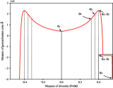
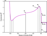
According to Theorem 2, the generalization error of the ensemble could be quantified by the diversity. Eq. (30) reflects the relationship of individual classifiers $\mathop{\rm{div}}(f_{ens},\mathbf{x}^{*})\in(-\frac{1}{2},\frac{1}{2})$ and the performance of generalization error of the ensemble $R(\mathbf{w})$. Therefore, the first and the second derivative of the estimated risk $\hat{R}(\mathbf{w})$ could be obtained by taking the derivative of $\hat{R}(\mathbf{w})$ on $\mathop{\rm{div}}(f_{ens},\mathbf{x}^{*})$, i.e.,

$$\hat{R}^{\prime}= 4\left(\frac{8\delta}{1-2\varepsilon}\right)^{2}\frac{1}{(\lambda-2\mathop{\rm{div}}(f_{ens},\mathbf{x}^{*}))^{3}}$$

$$\cdot\log_{2}\left(8|S|\left(\frac{(1-2\varepsilon)(\lambda-2\mathop{\rm{div}}(f_{ens},\mathbf{x}^{*}))}{8\delta}\right)^{2}\right)\,,$$ (31)

$$\hat{R}^{\prime\prime}= \frac{8}{\ln 2}\left(\frac{8\delta}{1-2\varepsilon}\right)^{2}\frac{1}{(\lambda-2\mathop{\rm{div}}(f_{ens},\mathbf{x}^{*}))^{4}}$$

$$\cdot \left(3\ln\left(8|S|\left(\frac{(1-2\varepsilon)(\lambda-2\mathop{\rm{div}}(f_{ens},\mathbf{x}^{*}))}{8\delta}\right)^{2}\right)-2\right)\,.$$ (32)

We are already aware that $\mathop{\rm{div}}(f_{ens},\mathbf{x}^{*})\in(-\frac{1}{2},\frac{1}{2})$. Thus, the graph of the upper bound of the generalization error $\hat{R}(\mathbf{w})$ is symmetrical about the vertical axis, as shown in Figure 2. And then we take $\mathop{\rm{div}}(f_{ens},\mathbf{x}^{*})\in(0,\frac{1}{2})$ for example to analyze the effect of diversity on the generalization error in the ensemble.

Table I: Monotone intervals. The first column is diversity $\mathop{\rm{div}}(f_{ens},\mathbf{x}^{*})$. The second and the third columns are the estimated risk $\hat{R}(\mathbf{w})$ and its first derivative, respectively. Note that the estimated risk reflects the generalization error $R(\mathbf{w})$ of the ensemble $f_{ens}$. The fourth and the fifth columns are the variation of the estimated risk and that of its first derivative, respectively.

$\mathop{\rm{div}}(f_{ens},\mathbf{x}^{*})$	$\hat{R}(\mathbf{w})$	$\hat{R}^{\prime}(\mathbf{w})$	$\Delta\hat{R}$	$\Delta\hat{R}^{\prime}$
$(-q_{3},-q_{2})$	$\nearrow$ convex	$\searrow$ concave	smaller	larger
$(-q_{2},-q_{5})$	$\searrow$ convex	$\searrow$ concave	smaller	larger
$(-q_{5},-q_{6})$	$\searrow$ concave	$\nearrow$ concave	larger	larger
$(-q_{6},-q_{1})$	$\searrow$ concave	$\nearrow$ convex	larger	smaller
$(q_{1},q_{6})$	$\nearrow$ concave	$\nearrow$ concave	larger	larger
$(q_{6},q_{5})$	$\nearrow$ concave	$\nearrow$ convex	larger	smaller
$(q_{5},q_{2})$	$\nearrow$ convex	$\searrow$ convex	smaller	smaller
$(q_{2},q_{3})$	$\searrow$ convex	$\searrow$ convex	smaller	smaller

As the relationship between the proposed diversity $\mathop{\rm{div}}(f_{ens},\mathbf{x}^{*})$ and the generalization error $\hat{R}(\mathbf{w})$ in the ensemble is Eq. (30), the monotonicity and concavity of function could be analyzed based on its first derivative and second derivative. On the positive abscissa axis, let $q_{1}$ and $q_{3}$ be the left endpoint and the right endpoint of the range, respectively. The function’s inflecion point $q_{2}$ is found by making $\hat{R}^{\prime}(\mathbf{w})=0$ , also remarked as $q_{4}$ . Thus the monotone increasing interval is $(q_{1},q_{2})$ , and the monotone diminishing interval is $(q_{2},q_{3})$ . Then the stagnation point of the first derivative $q_{5}$ is found by making $\hat{R}^{\prime\prime}(\mathbf{w})=0$ , to analyze the concavity of the function $\hat{R}(\mathbf{w})$ ; the stagnation point of the second derivative $q_{6}$ is found by making $\hat{R}^{\prime\prime\prime}(\mathbf{w})=0$ , to analyze the concavity of the function $\hat{R}^{\prime}(\mathbf{w})$ . Their values are

$$q_{1}=\varepsilon\,,\;\;q_{3}= \frac{1}{2}\bigg{(}1-\frac{\varepsilon}{1-2\varepsilon}\bigg{)}\,,\quad\quad\quad\quad\,\,\,$$ (33a)

$$q_{4}=q_{2}= \frac{1}{2}\Bigg{(}1-\frac{\delta}{1-2\varepsilon}\sqrt{\frac{8}{|S|}}\,\Bigg{)}\,,\quad\quad\quad\,\,$$ (33b)

$$q_{5}= \frac{1}{2}\Bigg{(}1-\frac{\delta}{1-2\varepsilon}\sqrt{\frac{8}{|S|}e^{\frac{2}{3}}}\,\Bigg{)}\,,$$ (33c)

$$q_{6}= \frac{1}{2}\Bigg{(}1-\frac{\delta}{1-2\varepsilon}\sqrt{\frac{8}{|S|}e^{\frac{7}{6}}}\,\Bigg{)}\,,$$ (33d)

respectively, where an implied condition exists, i.e.,

$$\footnotesize\varepsilon\leqslant\frac{\delta}{1-2\varepsilon}\sqrt{\frac{8}{|S|}}\leqslant 1-2\varepsilon\,.$$ (34)

Note that $q_{1}<q_{2}<q_{3}$ and $q_{6}<q_{5}<q_{4}=q_{2}\,.$ Then the domain of diversity $\mathop{\rm{div}}(f_{ens},\mathbf{x}^{*})$ could be divided into eight intervals, as shown in Table I. Up to now, we could analyze in detail the effect of diversity on generalization error within different intervals.

1. When $\mathop{\rm{div}}(f_{ens},\mathbf{x}^{*})=0$ in this paper, we only consider two cases: “all individual classifiers give the right result of the instance $\mathbf{x}^{*}$’s label;” “all individual classifiers give the wrong result of the instance $\mathbf{x}^{*}$’s label.” We do not consider the situation of a tie.

2. In real situations, $\mathop{\rm{div}}(f_{ens},\mathbf{x}^{*})$ is negative in most cases which means that “the ensemble classifier has misclassified the instance that corresponds to the selected $\mathop{\rm{div}}(f_{ens},\mathbf{x}^{*})$.” Notice that in the finite experiments, when the value of $|S|$ satisfies Eq. (34), it is rare that $\mathop{\rm{div}}(f_{ens},\mathbf{x}^{*})$ is larger than zero. If $\mathop{\rm{div}}(f_{ens},\mathbf{x}^{*})<0\,,$ increasing diversity will improve the ensemble’s performance, which is the reason why we should increase diversity in that case.

3. When $\mathop{\rm{div}}(f_{ens},\mathbf{x}^{*})$ is located in the positive abscissa axis, the ensemble classifies the corresponding instance correctly. In the range near zero, individual classifiers that classify the instance correctly take great advantage, and the closer $\mathop{\rm{div}}(f_{ens},\mathbf{x}^{*})$ is to zero, the greater their advantage is. In the range near $1/2\,,$ individual classifiers that classify the instance correctly take little advantage, and the closer $\mathop{\rm{div}}(f_{ens},\mathbf{x}^{*})$ is to $1/2\,,$ the less their advantage is. In this case, diversity needs to be decreased to increase the generalization performance of the ensemble, with the basic idea of keeping the ensemble classifying the corresponding instance correctly. In summary, increasing diversity will reduce the advantage of the individuals that classify the instance correctly, which should be avoided.

4. When $\mathop{\rm{div}}(f_{ens},\mathbf{x}^{*})$ is located in the negative axis, the ensemble classifies the instance incorrectly. Similar results could be analogized.

Based on these analyses, the relationship between the proposed diversity and generalization error varies when diversity falls in different ranges. Generally speaking, there are two specific ranges that need to be paid attention to particularly, i.e., $(-q_{5},-q_{6})$ and $(-q_{6},-q_{1})\,,$ according to Table I. In these two ranges, more diversity would lead to better generalization, which is why it is necessary to increase $\mathop{\rm{div}}(f_{ens},\mathbf{x}^{*})$ to get a more effective ensemble classifier. However, in other ranges, it is not worth increasing diversity, and the ensemble could remain the same to continue the learning process.

III-D Ensemble Pruning based on Diversity and One Ensemble Pruning Framework

Inspired by the relationship between the proposed diversity and generalization of classification ensembles, we propose an ensemble pruning method, named as “Ensemble Pruning based on Diversity (EPBD),” presented in Algorithm 1. It aims to prune an ensemble with rare performance degradation, with the basic idea of utilizing diversity and accuracy simultaneously.

Algorithm 1 Ensemble Pruning based on Diversity (EPBD)

0:  A training set $S=\{(\mathbf{x}_{i},y_{i})|\,i\in[|S|]\}$, an original ensemble $F=\{f_{j}|\,j\in[|F|]\}$, and the threshold $\alpha$.

0:  The pruned sub-ensemble $H\,(H\subset F)$.

1:  $H=\emptyset$.

2:  repeat

3:     Search for the specific data instance $(\mathbf{x},y)$ which satisfies the search criterion Eq. (13).

4:     Sort classifiers in $F$ that classify this instance correctly in ascending order according to the accuracy performance.

5:     Move the top one $f(\cdot)$ in the previous step from $F$ to $H$ .

6:  until The termination condition is satisfied.

(a)

(b)

(c)

(d)

(e)

(f)

(g)

(h)

(i)

(j)

(k)

(l)

Figure 3: Relationship of the loss difference $-(\bar{G}-\bar{A})$ in Eq. (5) and different diversity measures, using Bagging to conduct ensemble classifiers and MLPs as individual classifiers. (a) Disagreement measure [49, 50]; (b) $Q$-statistic [47]; (c) Correlation coefficient [51]; (d) $\kappa$-statistic [48]; (e) Double-fault [52]; (f) Kohavi-Wolpert variance [54]; (g) Interrater agreement [53]; (h–i) The entropy of the votes [55, 56]; (j) The difficulty index [57, 28]; (k) The generalized diversity [58]; (l) The coincident failure diversity [58].

(a)

(b)

(c)

(d)

(e)

(f)

(g)

(h)

(i)

(j)

(k)

(l)

Figure 4: Relationship of the loss difference $-(\bar{G}-\bar{A})$ in Eq. (5) and different diversity measures, using AdaBoost to conduct ensemble classifiers and MLPs as individual classifiers. Diversity measures used in (a–l) refer to those in Figure 4.

The inputs of this method are: (i) a training set $S$ of valid data instances, (ii) a set $F$ of trained individual classifiers, i.e., the original set of classifiers to constitute an ensemble classifier in Eq. (1), and (iii) the ratio $\alpha$ which means the individual classifiers in the pruned sub-ensemble are chosen in a ratio of $\alpha(\%)$ from the original ensemble. Notice that all individual members are treated equally here, which means that $w_{i}=1/|F|,\,\forall\,i\in[|F|]$.

Algorithm 2 Ensemble Pruning Framework Utilizing the Trade-off Between Accuracy and Diversity (FTAD)

0:  A training set $S=\{(\mathbf{x}_{i},y_{i})\,|\,i\in[|S|]$, an original ensemble $F=\{f_{j}\,|\,j\in[|F|]$, an arbitrary diversity measure $DIV$, and the threshold $\alpha$.

0:  The pruned sub-ensemble $H\,(H\subset F)$.

1:  $H=\emptyset$.

2:  repeat

3:     Compute the diversity of the ensemble on each data instance using the specified diversity measure $DIV$, i.e., $DIV(\mathbf{x})$.

4:     Compute the margin of the ensemble on each data instance, i.e., $\lambda-2DIV(\mathbf{x})$, where $\lambda$ is defined in Eq. (13).

5:     Search for the specific data instance $(\mathbf{x},y)$, i.e., $\operatorname*{argmin}_{(\mathbf{x},y)\in S}\lambda-2DIV(\mathbf{x})$.

6:     Sort classifiers in $F$ that classify this instance correctly in ascending order according to the accuracy performance.

7:     Move the top one $f(\cdot)$ in the previous step from $F$ to $H$ .

8:  until The termination condition is satisfied.

For example, individual members in one ensemble generated by AdaBoost might have different values of weights in the combination, however, their weight coefficients would still be treated as important as each other in the pruning process, to simplify the analyses since it doesn’t talk more about the situation where the individual classifiers in the ensemble are not treated equally. The output of this method is the set of classifiers $H$ composing the pruned sub-ensemble after pruning, which is initially set to $\emptyset$. This algorithm terminates when the number of $H$ reaches the number of a pruned sub-ensemble classifier (i.e., $\alpha|F|$), or when it cannot pick up an individual classifier in $F$ that satisfies the corresponding condition (i.e., all individual classifiers in $F$ misclassify the corresponding instance).

The objective of this method is to obtain a pruned sub-ensemble that approaches the performance as optimal as possible. As shown in Algorithm 1, it firstly picks out an individual classifier considering diversity and accuracy simultaneously, raising diversity in line 3 and increasing accuracy in line 4. Specifically, the sorting principle we use in line 4 is mainly based on the accuracy performance of individual classifiers. Then it puts the selected individual classifier into the candidate classifier set $H$, as shown in line 5. Subsequently, it follows a cycle to select the expected classifiers in $F$ repeatedly until the termination conditions are met.

(a)

(b)

Figure 5: Relationship of the loss difference $-(\bar{G}-\bar{A})$ in Eq. (5) and the proposed diversity measure in Eq. (6), using MLPs as individual classifiers. (a) Using Bagging to conduct ensembles. (b) Using AdaBoost to conduct ensembles.

Moreover, inspired by the proposed ensemble pruning method (EPBD), we propose an ensemble pruning framework by utilizing the trade-off between accuracy and diversity, named as “Ensemble Pruning Framework Utilizing the Trade-off Between Accuracy and Diversity (FTAD),” presented in Algorithm 2. The diversity measure used in FTAD could be any existing diversity measure, such as $Q$-statistic or the disagreement measure. Note that EPBD is one particular case of FTAD by using the proposed diversity measure in this paper.

(a)

(b)

Figure 6: Relationship of error rate and estimated risk in Eq. (25) calculated based on diversity in Eq. (11) using bagging for binary classification. (a) Using NBs as individual classifiers. (b) Using LMs as individual classifiers.

III-E Complexity Analysis of EPBD

In this subsection, we give the complexity analysis of the proposed EPBD. According to the Algorithm 1, the computational complexity of EPBD is analyzed as follows:

• Firstly, the complexity of line 3 is $\mathcal{O}(jm+m\log{}m)$ where $j=n-i+1$, and $n,m$ are the number of individual classifiers and instances, respectively, when $i\in\{1,...,k\}$. Note that $k$ is the size of the pruned sub-ensemble.

• Secondly, the complexity of line 4 is $\mathcal{O}(j\log{}j)$ where $j=n-i+1$, when $i\in\{1,...,k\}$.

• Thirdly, the complexity of line 5 is $\mathcal{O}(1)$.

Therefore, the overall computational complexity of EPBD is $\mathcal{O}\big{(}\sum_{j=n-k+1}^{n}(jm+m\log{}m+j\log{}j)\big{)}$, i.e., $\mathcal{O}\big{(}km(n-\frac{k-1}{2})+km\log{}m+\sum_{i=n-k+1}^{n}(i\log{}i)\big{)}$.

(a)

(b)

Figure 7: Relationship of diversity and ensemble performance in Theorem 2, using bagging with DTs as individual classifiers for binary classification. (a) Relationship between the proposed diversity and error rate of the ensemble. (b) Relationship between the proposed diversity and the estimated risk in Eq. (25).

(a)

(b)

Figure 8: Relationship of diversity and ensemble performance in Theorem 2, using AdaBoost with LMs as individual classifiers for binary classification. (a) Relationship between the proposed diversity and error rate of the ensemble. (b) Relationship between the proposed diversity and the estimated risk in Eq. (25).

Table II: Comparison of the state-of-the-art pruning methods with EPBD using bagging to produce homogeneous ensembles. The column named “Ensem” is the corresponding result for the entire ensemble without pruning. The best accuracy with a lower standard deviation is indicated with bold fonts for each data set (row).

[b] Data Set Ensem ES KL KP OO DREP SEP PEP MRMR MRMC DiscEP TSP.AP TSP.DP GMA LCS EPBD waveform 89.09$\pm$1.27 84.34$\pm$8.76 83.48$\pm$8.39 83.48$\pm$8.39 89.47$\pm$0.40 89.35$\pm$0.66 89.03$\pm$0.83 89.19$\pm$0.81 88.43$\pm$0.94$\ddagger$ 89.43$\pm$0.82 89.37$\pm$0.38 89.71$\pm$0.75 88.19$\pm$0.95$\ddagger$ 88.51$\pm$1.29 88.95$\pm$1.37 89.53$\pm$0.48 heart 55.56$\pm$0.00 55.56$\pm$0.00 55.56$\pm$0.00 55.56$\pm$0.00 55.56$\pm$0.00 55.56$\pm$0.00 55.56$\pm$0.00 55.93$\pm$0.74 55.93$\pm$0.74 55.93$\pm$0.74 55.93$\pm$0.74 55.56$\pm$0.00 55.56$\pm$0.00 55.56$\pm$0.00 55.56$\pm$0.00 55.93$\pm$0.74 page 91.26$\pm$0.22$\ddagger$ 91.28$\pm$0.19 91.26$\pm$0.24 91.33$\pm$0.29 91.37$\pm$0.29 91.35$\pm$0.20 91.24$\pm$0.11 91.28$\pm$0.27 91.33$\pm$0.20 91.19$\pm$0.20$\ddagger$ 91.24$\pm$0.16 91.26$\pm$0.19 91.39$\pm$0.21 91.12$\pm$0.16$\ddagger$ 91.12$\pm$0.16$\ddagger$ 91.39$\pm$0.26 sensor (2d) 94.12$\pm$0.80$\ddagger$ 94.08$\pm$0.95$\ddagger$ 94.15$\pm$0.98 93.97$\pm$0.93$\ddagger$ 94.21$\pm$1.08 94.37$\pm$1.01 94.02$\pm$0.92$\ddagger$ 94.41$\pm$0.83 94.24$\pm$0.55 94.21$\pm$1.01 93.73$\pm$0.95$\ddagger$ 94.10$\pm$1.09 94.08$\pm$0.80 94.02$\pm$1.04$\ddagger$ 94.10$\pm$1.02 94.37$\pm$0.85 sensor (24d) 89.37$\pm$0.61 89.13$\pm$0.27 88.95$\pm$0.73 88.91$\pm$0.75 89.39$\pm$1.38 88.82$\pm$1.05$\ddagger$ 88.82$\pm$1.11$\ddagger$ 89.31$\pm$1.25 89.15$\pm$0.97 89.09$\pm$0.92 88.87$\pm$0.86 88.93$\pm$0.93$\ddagger$ 88.95$\pm$1.02 89.07$\pm$0.93 88.74$\pm$1.16 89.33$\pm$0.95 EEGEyeState 55.13$\pm$0.01 55.13$\pm$0.00 55.13$\pm$0.00 55.13$\pm$0.00 55.13$\pm$0.01 55.13$\pm$0.00 55.13$\pm$0.00 55.13$\pm$0.00 55.13$\pm$0.01 55.13$\pm$0.01 55.13$\pm$0.01 55.13$\pm$0.00 55.13$\pm$0.01 55.13$\pm$0.00 55.13$\pm$0.00 55.13$\pm$0.01 gmm (10d) 99.70$\pm$0.60 99.70$\pm$0.60 99.70$\pm$0.60 99.70$\pm$0.60 99.80$\pm$0.40 99.70$\pm$0.60 99.70$\pm$0.60 99.80$\pm$0.40 99.80$\pm$0.40 99.80$\pm$0.40 99.80$\pm$0.40 99.70$\pm$0.60 99.60$\pm$0.59 99.70$\pm$0.60 99.60$\pm$0.59 99.80$\pm$0.40 ames 61.17$\pm$4.01 58.54$\pm$7.61 55.77$\pm$6.67$\ddagger$ 56.50$\pm$4.72 59.71$\pm$6.93 57.96$\pm$5.57$\ddagger$ 58.54$\pm$4.53 59.85$\pm$5.28 59.12$\pm$4.21 57.66$\pm$3.72 61.61$\pm$4.49 60.44$\pm$4.78 59.71$\pm$6.04 56.50$\pm$2.64 59.56$\pm$3.53 61.02$\pm$5.80 wisconsin 96.89$\pm$0.55 96.44$\pm$0.55 96.44$\pm$0.86 96.89$\pm$0.73 96.59$\pm$1.00 96.59$\pm$0.76 96.00$\pm$0.59 96.44$\pm$0.98 96.74$\pm$0.76 96.89$\pm$1.09 97.04$\pm$0.47 96.74$\pm$1.00 96.89$\pm$0.55 96.59$\pm$0.36 96.89$\pm$0.30 96.89$\pm$0.73 ecoli 95.76$\pm$2.23 95.76$\pm$2.42 95.76$\pm$2.42 95.76$\pm$2.42 95.76$\pm$2.42 95.76$\pm$2.42 95.76$\pm$2.42 96.36$\pm$2.06 96.36$\pm$2.06 95.76$\pm$2.23 95.76$\pm$2.23 95.76$\pm$2.23 95.76$\pm$2.42 96.06$\pm$2.06 96.06$\pm$2.27 96.36$\pm$2.06 liver 62.90$\pm$2.98$\ddagger$ 61.16$\pm$2.49 62.03$\pm$5.75 65.22$\pm$2.43 63.77$\pm$3.04 65.51$\pm$3.60 64.64$\pm$3.38 66.38$\pm$2.96 65.80$\pm$2.98 63.19$\pm$2.98 62.90$\pm$2.84 61.74$\pm$2.98 64.93$\pm$3.82 61.45$\pm$6.12 61.74$\pm$4.36$\ddagger$ 66.96$\pm$3.36 yeast 69.59$\pm$4.61 67.77$\pm$2.86$\ddagger$ 67.70$\pm$2.36$\ddagger$ 69.39$\pm$1.66 69.73$\pm$3.27 65.41$\pm$2.60$\ddagger$ 69.80$\pm$4.23 69.39$\pm$3.44 69.86$\pm$3.06 69.12$\pm$2.89 68.24$\pm$3.82$\ddagger$ 68.58$\pm$3.15 68.72$\pm$3.44 67.36$\pm$3.66$\ddagger$ 68.45$\pm$3.95 70.54$\pm$2.92 sonar 80.00$\pm$6.62 76.59$\pm$5.69 78.05$\pm$6.90 79.02$\pm$6.28 80.49$\pm$6.54 80.00$\pm$5.85 79.51$\pm$3.65 79.51$\pm$5.89 81.95$\pm$8.10 80.49$\pm$6.36 76.10$\pm$4.97 79.02$\pm$3.31 76.10$\pm$6.79 79.51$\pm$7.49 80.49$\pm$6.17 80.49$\pm$7.07 wilt 93.90$\pm$1.34 93.71$\pm$1.49 94.37$\pm$0.85 93.34$\pm$1.51 94.33$\pm$0.87 92.12$\pm$1.81$\ddagger$ 93.90$\pm$1.44 93.59$\pm$1.59 94.33$\pm$0.98 94.35$\pm$0.93 94.00$\pm$1.25 94.46$\pm$0.95 93.86$\pm$1.00 93.92$\pm$1.44 93.75$\pm$1.17 94.48$\pm$0.87 spam 78.67$\pm$3.44 78.54$\pm$2.74 77.34$\pm$2.18 73.32$\pm$5.74 74.56$\pm$6.96 79.09$\pm$2.84 77.87$\pm$1.39 79.61$\pm$2.67 79.04$\pm$2.80 72.82$\pm$8.46 78.91$\pm$3.13 79.76$\pm$2.42 77.87$\pm$3.55 73.93$\pm$5.00 77.39$\pm$1.58 79.80$\pm$2.41 landsat 96.25$\pm$0.63 96.31$\pm$0.63 95.57$\pm$0.98 95.30$\pm$1.02 96.27$\pm$0.58 95.68$\pm$0.84 96.31$\pm$0.54 95.96$\pm$0.91 96.22$\pm$0.56 95.65$\pm$1.16 96.22$\pm$0.61 96.33$\pm$0.50 95.69$\pm$0.90 96.13$\pm$0.75 96.07$\pm$0.58 96.27$\pm$0.65 $t$-test (W/T/L) 3/13/0 2/14/0 2/14/0 1/15/0 0/16/0 4/12/0 2/14/0 0/16/0 1/15/0 1/15/0 2/14/0 1/15/0 1/15/0 4/12/0 2/14/0 — Average Rank 7.47 10.84 11.47 11.03 6.00 9.41 9.78 6.56 5.13 7.88 8.28 8.22 9.28 11.44 10.69 2.53

• The reported results are the average test accuracy (%) of each method and the corresponding standard deviation under 5-fold cross-validation on each data set.

• By two-tailed paired $t$-test at 5% significance level, $\ddagger$ and $\dagger$ denote that the performance of EPBD is superior to and inferior to that of the comparative method, respectively.

• The last two rows show the results of $t$-test and average rank, respectively. The “W/T/L” in $t$-test indicates that EPBD is superior to, not significantly different from, or inferior to the corresponding comparative methods. The average rank is calculated according to the Friedman test [102].

Table III: Comparison of the state-of-the-art pruning methods with EPBD using AdaBoost to produce homogeneous ensembles. The column named “Ensem” is the corresponding result for the entire ensemble without pruning. The best accuracy with a lower standard deviation is indicated with bold fonts for each data set (row).

[b] Data Set Ensem ES KL KP OO DREP SEP PEP MRMR MRMC DiscEP TSP.AP TSP.DP GMA LCS EPBD spam 79.33$\pm$2.04 81.44$\pm$1.58 79.39$\pm$3.15 78.32$\pm$2.76 79.17$\pm$2.23 79.91$\pm$1.44 79.06$\pm$2.90 81.85$\pm$1.36 81.44$\pm$1.58 78.78$\pm$2.24 78.78$\pm$2.24 79.04$\pm$2.11 76.63$\pm$2.51 73.54$\pm$6.13 79.04$\pm$2.11 79.98$\pm$2.12 credit 77.96$\pm$0.06 77.93$\pm$0.06 77.93$\pm$0.13 77.91$\pm$0.12 77.99$\pm$0.08 77.99$\pm$0.09 77.93$\pm$0.09 77.95$\pm$0.08 77.98$\pm$0.14 77.98$\pm$0.09 77.96$\pm$0.14 77.91$\pm$0.13 77.88$\pm$0.11$\ddagger$ 77.86$\pm$0.10 77.95$\pm$0.06 78.03$\pm$0.10 page 90.40$\pm$0.12$\ddagger$ 90.35$\pm$0.26$\ddagger$ 90.40$\pm$0.27$\ddagger$ 90.29$\pm$0.33$\ddagger$ 90.93$\pm$0.32 90.99$\pm$0.24 90.49$\pm$0.32 90.88$\pm$0.35 90.60$\pm$0.25 90.93$\pm$0.32 90.91$\pm$0.31 90.99$\pm$0.24 90.22$\pm$0.42$\ddagger$ 90.80$\pm$0.32 90.77$\pm$0.38 90.99$\pm$0.24 shuttle 96.75$\pm$0.08$\ddagger$ 97.33$\pm$0.06$\ddagger$ 97.33$\pm$0.06$\ddagger$ 92.40$\pm$2.09$\ddagger$ 97.81$\pm$0.10 97.70$\pm$0.05$\ddagger$ 94.75$\pm$2.43 96.80$\pm$2.10 97.85$\pm$0.05 97.65$\pm$0.10$\ddagger$ 97.85$\pm$0.05 97.85$\pm$0.05 92.05$\pm$2.09$\ddagger$ 97.59$\pm$0.12$\ddagger$ 97.85$\pm$0.05 97.85$\pm$0.05 wilt 94.64$\pm$0.04 94.66$\pm$0.08 94.66$\pm$0.08 94.66$\pm$0.08 94.66$\pm$0.08 94.66$\pm$0.08 94.62$\pm$0.00 94.62$\pm$0.00 94.71$\pm$0.10 94.66$\pm$0.08 94.71$\pm$0.10 94.71$\pm$0.10 94.71$\pm$0.10 94.66$\pm$0.08 94.71$\pm$0.10 94.71$\pm$0.10 segmentation 67.40$\pm$0.56 65.93$\pm$0.67$\ddagger$ 65.19$\pm$1.24$\ddagger$ 63.94$\pm$0.95$\ddagger$ 67.14$\pm$1.14 68.14$\pm$1.07$\dagger$ 66.02$\pm$1.79 66.32$\pm$3.21 65.89$\pm$0.87$\ddagger$ 65.71$\pm$0.95$\ddagger$ 66.67$\pm$0.43 66.28$\pm$0.73 65.50$\pm$1.66 66.15$\pm$0.67 66.54$\pm$0.45 66.80$\pm$0.56 iono 81.43$\pm$1.56 77.71$\pm$5.16 78.00$\pm$7.15 80.57$\pm$5.16 84.29$\pm$3.61 83.71$\pm$3.68 80.57$\pm$6.43 81.43$\pm$6.32 82.57$\pm$3.43 82.00$\pm$5.90 82.57$\pm$2.77 82.57$\pm$2.77 76.00$\pm$6.29 72.86$\pm$4.52$\ddagger$ 80.57$\pm$5.16 84.00$\pm$2.91 wilt 97.17$\pm$0.24 96.38$\pm$0.52 97.35$\pm$0.38 95.37$\pm$1.25$\ddagger$ 97.29$\pm$0.65 97.35$\pm$0.38 97.13$\pm$0.56 97.31$\pm$0.44 97.27$\pm$0.29 97.25$\pm$0.51 97.37$\pm$0.40 97.35$\pm$0.38 96.34$\pm$1.28 97.35$\pm$0.38 97.13$\pm$0.48 97.35$\pm$0.38 ecoli 69.70$\pm$2.71 64.24$\pm$4.35 62.73$\pm$4.94 63.33$\pm$3.76 66.36$\pm$6.24 64.55$\pm$3.26 63.94$\pm$3.76 63.03$\pm$4.75 64.55$\pm$3.12 61.82$\pm$4.64 60.91$\pm$8.10 66.06$\pm$6.82 65.15$\pm$1.66 64.55$\pm$4.94 62.73$\pm$4.66 67.27$\pm$4.85 yeast 63.45$\pm$1.90 66.15$\pm$2.35 63.24$\pm$1.94 63.31$\pm$1.04 63.78$\pm$2.80 60.61$\pm$2.65 61.96$\pm$1.46 63.18$\pm$2.73 62.84$\pm$3.64 62.64$\pm$3.29 62.50$\pm$2.87 63.18$\pm$2.79 59.80$\pm$3.74 62.09$\pm$2.85 62.50$\pm$2.45 63.78$\pm$3.60 ringnorm 68.32$\pm$1.27$\ddagger$ 68.67$\pm$1.21 68.21$\pm$1.69 67.88$\pm$0.68$\ddagger$ 69.20$\pm$0.90 69.86$\pm$1.31 67.05$\pm$1.40$\ddagger$ 68.55$\pm$1.22 69.17$\pm$0.82 68.53$\pm$1.03 68.88$\pm$1.10 69.32$\pm$1.04 68.15$\pm$1.22$\ddagger$ 68.80$\pm$0.86 68.86$\pm$0.77 69.17$\pm$0.92 waveform 83.46$\pm$0.60 83.00$\pm$0.64 82.52$\pm$0.62 81.72$\pm$1.11$\ddagger$ 82.78$\pm$1.21 83.26$\pm$0.78 82.82$\pm$1.03$\ddagger$ 82.86$\pm$0.74 83.44$\pm$0.19 83.14$\pm$1.14 82.40$\pm$0.94$\ddagger$ 82.90$\pm$0.30$\ddagger$ 82.80$\pm$1.05 82.32$\pm$0.67$\ddagger$ 82.54$\pm$0.47$\ddagger$ 83.86$\pm$0.74 gmm (10d) 99.70$\pm$0.25 99.80$\pm$0.25 95.58$\pm$5.24 97.59$\pm$4.58 99.70$\pm$0.25 99.60$\pm$0.38 99.70$\pm$0.60 99.80$\pm$0.25 97.39$\pm$4.48 99.60$\pm$0.38 97.49$\pm$4.53 99.50$\pm$0.32 99.50$\pm$0.32 99.70$\pm$0.25 99.60$\pm$0.38 99.80$\pm$0.25 $t$-test (W/T/L) 3/10/0 3/10/0 3/10/0 6/7/0 0/13/0 1/11/1 2/11/0 0/13/0 1/12/0 2/11/0 1/12/0 1/12/0 4/9/0 3/10/0 1/12/0 — Average Rank 7.62 8.85 10.96 13.15 5.35 5.42 11.19 8.08 6.58 9.23 8.04 6.35 12.77 10.58 9.15 2.69

(a)

(b)

(c)

(d)

Figure 9: Comparison of the state-of-the-art methods with EPBD on the test accuracy, using bagging to produce homogeneous ensembles. (a) Friedman test chart (non-overlapping means significant difference) [102]. (b) The aggregated rank for each pruning method (the smaller the better) [81]. (c) The aggregated time cost for each method. (d) The aggregated space cost for each method.

(a)

(b)

(c)

(d)

Figure 10: Comparison of the state-of-the-art methods with EPBD on the test accuracy, using AdaBoost to produce homogeneous ensembles. (a) Friedman test chart (non-overlapping means significant difference) [102]. (b) The aggregated rank for each pruning method (the smaller the better) [81]. (c) The aggregated time cost for each method. (d) The aggregated space cost for each method.

IV Experiments

In this section, we elaborate on our experiments to evaluate the proposed relationship between the proposed diversity and ensemble generalization performance and the proposed algorithms. The data sets we use include one image data set with $12,500$ pictures (Dogs vs Cats) and $28$ data sets from UCI repository [103]. Standard $5$-fold cross-validation is used in these experiments, i.e., in each iteration, the entire data set is split into two parts, with $80\%$ as the training set and $20\%$ as the test set. Bagging [38] and AdaBoost [104, 41] are used to constitute an ensemble classifier on various kinds of individual classifiers including decision trees (DT), naive Bayesian (NB) classifiers, $k$-nearest neighbors (KNN) classifiers, linear model (LM) classifiers, linear SVMs (LSVM), support vector machines (SVM), and multilayer perceptrons (MLP). We evaluate the proposed relationship between the proposed diversity and ensemble performance using scatter diagrams with their correlation. Besides, to evaluate our proposed pruning method EPBD, the baselines we considered are a variety of ranking-based methods, namely Early Stopping (ES), KL-divergence pruning (KL), Kappa pruning (KP) [69], orientation ordering pruning (OO) [105], diversity regularized ensemble pruning (DREP) [35], accuracy-based ensemble pruning (TSP.AP) [73], and diversity-based ensemble pruning (TSP.DP) [73] as well as optimization-based methods, namely single-objective ensemble pruning (SEP), and Pareto ensemble pruning (PEP) [81], the maximal relevant minimal redundant (MRMR) method [82], the maximal relevancy miximum complementary (MRMC) method [82], and the discriminative ensemble pruning (DiscEP) [83]. Moreover, we adopt two methods from diversity maximization via composable coresets [106, 107] and change them slightly to make them suitable for pruning problems, namely the Gonzalez’s algorithm (GMA) and local search algorithm (LCS). An ensemble is trained and pruned on the training set and then evaluated on the test set. It is worth mentioning that several methods (such as OO, DREP, SEP, PEP, LCS, and TSP.AP) cannot fix the number of classifiers after ensemble pruning, while others could do that by giving a pruning rate that is the up limit of the percentage of those discarded individual classifiers in the original ensemble. Those methods that cannot fix the size of the pruned sub-ensemble might lead to increasing or reducing the size of pruned sub-ensembles and affect their space cost.

Table IV: Comparison of different diversity measures with FTAD using bagging to produce an ensemble with NBs as individual classifiers. The column named “Ensem” is the corresponding result for the entire ensemble without pruning. The best accuracy with a lower standard deviation is indicated with bold fonts for each data set (row).

[b] Data Set Ensem Disag QStat Corre KStat DoubF KWVar Inter EntCC EntSK Diffi GeneD CFail EPBD ames 57.37$\pm$3.53$\ddagger$ 59.71$\pm$4.39 59.12$\pm$4.36 59.12$\pm$4.36 59.12$\pm$4.36 58.69$\pm$4.07 59.12$\pm$4.36 59.12$\pm$4.36 58.39$\pm$4.08 58.39$\pm$4.08 59.12$\pm$4.36 58.69$\pm$4.07 58.69$\pm$4.07 58.69$\pm$4.07 card 79.56$\pm$4.48 79.42$\pm$5.57 79.12$\pm$5.03 79.12$\pm$5.03 79.12$\pm$5.03 79.42$\pm$5.57 79.42$\pm$5.57 79.42$\pm$5.57 79.56$\pm$5.44 79.56$\pm$5.44 79.12$\pm$5.03 79.42$\pm$5.57 79.42$\pm$4.85 79.42$\pm$5.57 heart 84.07$\pm$3.23 84.44$\pm$1.89 84.07$\pm$2.22 84.07$\pm$2.22 84.07$\pm$2.22 83.70$\pm$2.72 84.07$\pm$3.01 84.07$\pm$3.01 83.70$\pm$2.72 83.70$\pm$2.72 84.07$\pm$2.22 83.70$\pm$2.72 83.70$\pm$2.72 83.70$\pm$2.72 ringnorm 98.69$\pm$0.24 98.66$\pm$0.25 98.66$\pm$0.25 98.66$\pm$0.25 98.66$\pm$0.25 98.66$\pm$0.25 98.66$\pm$0.25 98.66$\pm$0.25 98.66$\pm$0.25 98.66$\pm$0.25 98.66$\pm$0.25 98.66$\pm$0.25 98.66$\pm$0.25 98.66$\pm$0.25 wisconsin 96.00$\pm$1.11 96.00$\pm$1.37 96.00$\pm$1.37 96.00$\pm$1.37 96.00$\pm$1.37 96.00$\pm$1.37 96.00$\pm$1.37 96.00$\pm$1.37 96.00$\pm$1.37 96.00$\pm$1.37 96.00$\pm$1.37 96.00$\pm$1.37 96.00$\pm$1.37 96.00$\pm$1.37 landsat 90.30$\pm$0.73 90.48$\pm$0.73 90.48$\pm$0.73 90.48$\pm$0.73 90.48$\pm$0.73 90.48$\pm$0.73 90.48$\pm$0.73 90.48$\pm$0.73 90.47$\pm$0.71 90.48$\pm$0.73 90.48$\pm$0.73 90.48$\pm$0.73 90.47$\pm$0.71 90.48$\pm$0.73 shuttle 89.48$\pm$0.16$\ddagger$ 89.71$\pm$0.14 89.71$\pm$0.14 89.71$\pm$0.14 89.71$\pm$0.14 89.71$\pm$0.14 89.71$\pm$0.14 89.71$\pm$0.14 89.71$\pm$0.14 89.71$\pm$0.14 89.71$\pm$0.14 89.71$\pm$0.14 89.71$\pm$0.14 89.71$\pm$0.14 ecoli 92.12$\pm$2.78 92.42$\pm$3.46 92.42$\pm$3.46 92.42$\pm$3.46 92.42$\pm$3.46 94.24$\pm$2.61 92.42$\pm$3.46 92.42$\pm$3.46 92.42$\pm$3.46 92.42$\pm$3.46 92.42$\pm$3.46 92.42$\pm$3.46 92.42$\pm$3.46 94.24$\pm$2.61 yeast 58.24$\pm$2.64$\ddagger$ 60.20$\pm$1.67 57.30$\pm$3.33 57.30$\pm$3.33 57.30$\pm$3.33 61.82$\pm$1.46 61.82$\pm$1.46 61.82$\pm$1.46 60.27$\pm$1.64 60.20$\pm$1.67 57.30$\pm$3.33 61.69$\pm$1.70 61.49$\pm$1.61 61.82$\pm$1.46 mammo_graphic 80.73$\pm$3.04 79.79$\pm$2.76 79.69$\pm$2.57 79.69$\pm$2.57 79.69$\pm$2.57 79.58$\pm$2.72 79.48$\pm$2.61 79.48$\pm$2.61 79.79$\pm$2.76 79.79$\pm$2.76 79.69$\pm$2.57 79.58$\pm$2.72 79.58$\pm$2.72 79.58$\pm$2.72 madelon 58.85$\pm$2.37 58.96$\pm$2.28 59.19$\pm$1.31 59.19$\pm$1.31 59.19$\pm$1.31 59.04$\pm$2.07 59.04$\pm$2.07 59.04$\pm$2.07 59.58$\pm$2.39 58.96$\pm$2.28 59.19$\pm$1.31 59.04$\pm$2.07 58.92$\pm$2.22 59.04$\pm$2.07 sensor (2d) 81.41$\pm$0.86 81.61$\pm$0.91 81.81$\pm$0.57 81.81$\pm$0.57 81.81$\pm$0.57 82.02$\pm$0.70 81.81$\pm$0.57 81.81$\pm$0.57 81.59$\pm$0.93 81.61$\pm$0.91 81.81$\pm$0.57 82.02$\pm$0.70 81.92$\pm$0.76 82.02$\pm$0.70 sensor (4d) 74.57$\pm$0.88$\ddagger$ 75.44$\pm$0.99 75.55$\pm$0.89 75.55$\pm$0.89 75.55$\pm$0.89 75.55$\pm$0.89 75.55$\pm$0.89 75.55$\pm$0.89 75.33$\pm$0.85 75.44$\pm$0.99 75.55$\pm$0.89 75.55$\pm$0.89 75.51$\pm$0.94 75.55$\pm$0.89 waveform 85.29$\pm$0.95 85.35$\pm$0.94 85.33$\pm$0.92 85.33$\pm$0.92 85.33$\pm$0.92 85.33$\pm$0.92 85.33$\pm$0.92 85.33$\pm$0.92 85.35$\pm$0.91 85.35$\pm$0.94 85.33$\pm$0.92 85.33$\pm$0.92 85.33$\pm$0.92 85.33$\pm$0.92 $t$-test (W/T/L) 4/10/0 0/14/0 0/14/0 0/14/0 0/14/0 0/14/0 0/14/0 0/14/0 0/14/0 0/14/0 0/14/0 0/14/0 0/14/0 — Average Rank 9.89 6.71 7.21 7.21 7.21 6.79 7.21 7.21 7.68 7.86 7.21 7.43 8.57 6.79

• The reported results are the average test accuracy (%) of each method and the corresponding standard deviation under 5-fold cross-validation on each data set.

• By two-tailed paired $t$-test at 5% significance level, $\ddagger$ and $\dagger$ denote that the performance of EPBD is superior to and inferior to that of the comparative method, respectively.

• The last two rows show the results of $t$-test and average rank, respectively. The “W/T/L” in $t$-test indicates that EPBD is superior to, not significantly different from, or inferior to the corresponding comparative methods. The average rank is calculated according to the Friedman test [102].

Table V: Comparison of different diversity measures with FTAD using bagging to produce an ensemble with KNNs as individual classifiers. The column named “Ensem” is the corresponding result for the entire ensemble without pruning. The best accuracy with a lower standard deviation is indicated with bold fonts for each data set (row).

[b] Data Set Ensem Disag QStat Corre KStat DoubF KWVar Inter EntCC EntSK Diffi GeneD CFail EPBD gmm (2d) 96.90$\pm$0.63 96.92$\pm$0.66 96.97$\pm$0.66 96.97$\pm$0.66 96.97$\pm$0.66 96.97$\pm$0.66 96.97$\pm$0.66 96.97$\pm$0.66 96.92$\pm$0.66 96.92$\pm$0.66 96.97$\pm$0.66 96.97$\pm$0.66 96.97$\pm$0.66 96.97$\pm$0.66 card 67.74$\pm$2.33 68.03$\pm$2.67 67.74$\pm$3.28 67.74$\pm$3.28 67.74$\pm$3.28 68.91$\pm$2.83 68.91$\pm$2.83 68.91$\pm$2.83 67.88$\pm$2.85 68.03$\pm$2.67 67.74$\pm$3.28 68.32$\pm$2.15 68.91$\pm$2.83 68.91$\pm$2.83 liver 64.06$\pm$4.62 62.61$\pm$5.45 63.48$\pm$5.53 63.48$\pm$5.53 63.48$\pm$5.53 64.35$\pm$4.36 63.19$\pm$6.77 63.19$\pm$6.77 62.61$\pm$5.45 62.61$\pm$5.45 63.48$\pm$5.53 62.61$\pm$6.94 63.48$\pm$5.53 64.35$\pm$4.36 credit 74.18$\pm$0.35$\ddagger$ 74.69$\pm$0.44 74.63$\pm$0.45 74.63$\pm$0.45 74.63$\pm$0.45 74.72$\pm$0.35 74.72$\pm$0.35 74.72$\pm$0.35 74.70$\pm$0.44 74.69$\pm$0.44 74.63$\pm$0.45 74.72$\pm$0.35 74.62$\pm$0.31 74.72$\pm$0.35 page 95.96$\pm$0.35 96.11$\pm$0.34 96.11$\pm$0.29 96.11$\pm$0.29 96.11$\pm$0.29 96.11$\pm$0.29 96.11$\pm$0.29 96.11$\pm$0.29 96.11$\pm$0.34 96.11$\pm$0.34 96.11$\pm$0.29 96.11$\pm$0.29 96.11$\pm$0.29 96.11$\pm$0.29 shuttle 99.84$\pm$0.03 99.83$\pm$0.02 99.83$\pm$0.03 99.83$\pm$0.03 99.83$\pm$0.03 99.83$\pm$0.03 99.83$\pm$0.03 99.83$\pm$0.03 99.83$\pm$0.02 99.83$\pm$0.02 99.83$\pm$0.03 99.83$\pm$0.03 99.83$\pm$0.03 99.83$\pm$0.03 wilt 98.01$\pm$0.50 97.97$\pm$0.54 97.81$\pm$0.34 97.81$\pm$0.34 97.81$\pm$0.34 98.04$\pm$0.38 97.75$\pm$0.34 97.75$\pm$0.34 97.97$\pm$0.54 97.97$\pm$0.54 97.81$\pm$0.34 97.91$\pm$0.48 97.95$\pm$0.47 98.04$\pm$0.38 ecoli 96.36$\pm$1.55 95.76$\pm$1.13 95.76$\pm$1.13 95.76$\pm$1.13 95.76$\pm$1.13 95.76$\pm$1.13 95.76$\pm$1.13 95.76$\pm$1.13 95.76$\pm$1.13 95.76$\pm$1.13 95.76$\pm$1.13 95.76$\pm$1.13 95.76$\pm$1.13 95.76$\pm$1.13 mammo_graphic 77.71$\pm$2.70 78.02$\pm$2.76 77.92$\pm$2.90 77.92$\pm$2.90 77.92$\pm$2.90 77.92$\pm$2.90 77.92$\pm$2.90 77.92$\pm$2.90 78.12$\pm$2.81 78.02$\pm$2.76 77.92$\pm$2.90 77.92$\pm$2.90 77.71$\pm$3.06 77.92$\pm$2.90 madelon 70.38$\pm$2.21 70.46$\pm$1.96 69.69$\pm$2.05 69.69$\pm$2.05 69.69$\pm$2.05 70.31$\pm$1.89 69.92$\pm$1.58 69.92$\pm$1.58 70.15$\pm$1.96 70.46$\pm$1.96 69.69$\pm$2.05 70.31$\pm$1.89 70.35$\pm$1.94 70.31$\pm$1.89 sensor (4d) 96.99$\pm$0.50 96.83$\pm$0.45 96.98$\pm$0.43 96.98$\pm$0.43 96.98$\pm$0.43 96.98$\pm$0.43 96.98$\pm$0.43 96.98$\pm$0.43 96.87$\pm$0.43 96.83$\pm$0.45 96.98$\pm$0.43 96.98$\pm$0.43 96.98$\pm$0.43 96.98$\pm$0.43 sensor (24d) 88.82$\pm$0.78 88.78$\pm$0.74 88.43$\pm$0.66 88.43$\pm$0.66 88.43$\pm$0.66 88.56$\pm$0.57 88.56$\pm$0.57 88.56$\pm$0.57 88.74$\pm$0.75 88.78$\pm$0.74 88.43$\pm$0.66 88.56$\pm$0.57 88.56$\pm$0.57 88.56$\pm$0.57 waveform 85.03$\pm$0.83 85.09$\pm$0.60 85.07$\pm$0.78 85.07$\pm$0.78 85.07$\pm$0.78 85.19$\pm$0.53 85.15$\pm$0.57 85.15$\pm$0.57 85.05$\pm$0.63 85.09$\pm$0.60 85.07$\pm$0.78 85.07$\pm$0.32 85.17$\pm$0.26 85.19$\pm$0.53 EEGEyeState 96.72$\pm$0.20$\dagger$ 96.37$\pm$0.21 96.24$\pm$0.24 96.24$\pm$0.24 96.24$\pm$0.24 96.38$\pm$0.15 96.38$\pm$0.15 96.38$\pm$0.15 96.37$\pm$0.21 96.37$\pm$0.21 96.24$\pm$0.24 96.38$\pm$0.15 96.38$\pm$0.15 96.38$\pm$0.15 $t$-test (W/T/L) 1/12/1 0/14/0 0/14/0 0/14/0 0/14/0 0/14/0 0/14/0 0/14/0 0/14/0 0/14/0 0/14/0 0/14/0 0/14/0 — Average Rank 6.64 7.68 9.18 9.18 9.18 5.00 6.89 6.89 8.50 7.68 9.18 7.18 6.82 5.00

Table VI: Comparison of different diversity measures with FTAD using AdaBoost to produce an ensemble with SVMs as individual classifiers. The column named “Ensem” is the corresponding result for the entire ensemble without pruning. The best accuracy with a lower standard deviation is indicated with bold fonts for each data set (row).

[b] Data Set Ensem Disag QStat Corre KStat DoubF KWVar Inter EntCC EntSK Diffi GeneD CFail EPBD gmm (10d) 99.80$\pm$0.25 99.80$\pm$0.40 99.80$\pm$0.40 99.80$\pm$0.40 99.80$\pm$0.40 99.80$\pm$0.40 99.80$\pm$0.40 99.80$\pm$0.40 99.80$\pm$0.40 99.80$\pm$0.40 99.80$\pm$0.40 99.80$\pm$0.40 99.80$\pm$0.40 99.80$\pm$0.40 sonar 62.93$\pm$3.90 64.39$\pm$4.25 64.39$\pm$7.96 64.39$\pm$7.96 64.39$\pm$7.96 62.44$\pm$4.25 65.85$\pm$7.40 65.85$\pm$7.40 61.46$\pm$4.47 61.95$\pm$5.69 64.39$\pm$7.96 65.85$\pm$7.40 65.85$\pm$7.40 66.83$\pm$7.00 waveform 88.21$\pm$0.50$\ddagger$ 89.97$\pm$0.52 89.81$\pm$0.48$\ddagger$ 89.81$\pm$0.48$\ddagger$ 89.81$\pm$0.48$\ddagger$ 89.51$\pm$0.77$\ddagger$ 89.51$\pm$0.77$\ddagger$ 89.51$\pm$0.77$\ddagger$ 89.97$\pm$0.52 89.97$\pm$0.52 89.81$\pm$0.48$\ddagger$ 89.51$\pm$0.77$\ddagger$ 89.51$\pm$0.77$\ddagger$ 90.71$\pm$0.75 landsat 65.24$\pm$0.00 65.24$\pm$0.00 65.24$\pm$0.00 65.24$\pm$0.00 65.24$\pm$0.00 65.24$\pm$0.00 65.24$\pm$0.00 65.24$\pm$0.00 65.24$\pm$0.00 65.24$\pm$0.00 65.24$\pm$0.00 65.24$\pm$0.00 65.24$\pm$0.00 65.24$\pm$0.00 page 90.59$\pm$0.21 90.99$\pm$0.51 90.95$\pm$0.48 90.95$\pm$0.48 90.95$\pm$0.48 90.95$\pm$0.48 90.95$\pm$0.48 90.95$\pm$0.48 90.86$\pm$0.49 90.86$\pm$0.49 90.95$\pm$0.48 90.95$\pm$0.48 90.97$\pm$0.44 90.99$\pm$0.41 shuttle 97.12$\pm$0.15 97.28$\pm$0.18 97.28$\pm$0.16 97.28$\pm$0.16 97.28$\pm$0.16 97.28$\pm$0.16 97.28$\pm$0.16 97.28$\pm$0.16 97.28$\pm$0.18 97.28$\pm$0.18 97.28$\pm$0.16 97.28$\pm$0.16 97.28$\pm$0.16 95.25$\pm$2.08 yeast 65.00$\pm$1.14 55.41$\pm$12.42 55.41$\pm$12.42 55.41$\pm$12.42 55.41$\pm$12.42 54.93$\pm$12.09 54.93$\pm$12.09 54.93$\pm$12.09 59.80$\pm$9.89 59.93$\pm$9.93 55.41$\pm$12.42 54.93$\pm$12.09 45.20$\pm$10.17$\ddagger$ 65.07$\pm$1.18 sensor (4d) 85.63$\pm$0.90 84.47$\pm$0.78 84.00$\pm$1.45 84.00$\pm$1.45 84.00$\pm$1.45 77.58$\pm$8.33 84.01$\pm$0.85 84.01$\pm$0.85 84.47$\pm$0.78 84.47$\pm$0.78 84.00$\pm$1.45 81.21$\pm$7.51 81.28$\pm$7.54 84.01$\pm$0.85 EEGEyeState 55.13$\pm$0.00 55.13$\pm$0.00 55.13$\pm$0.00 55.13$\pm$0.00 55.13$\pm$0.00 55.13$\pm$0.00 55.13$\pm$0.00 55.13$\pm$0.00 55.13$\pm$0.00 55.13$\pm$0.00 55.13$\pm$0.00 55.13$\pm$0.00 55.13$\pm$0.00 55.13$\pm$0.00 $t$-test (W/T/L) 1/8/0 0/9/0 1/8/0 1/8/0 1/8/0 1/8/0 1/8/0 1/8/0 0/9/0 0/9/0 1/8/0 1/8/0 2/7/0 — Average Rank 9.33 5.39 7.56 7.56 7.56 9.56 7.72 7.72 6.72 6.50 7.56 8.50 8.17 5.17

(a)

(b)

(c)

(d)

Figure 11: Comparison of various diversity measures with FTAD and EPBD on the test accuracy, using bagging to produce homogeneous ensembles. (a) Friedman test chart (non-overlapping means significant difference) [102]. (b) The aggregated rank for each diversity measure (the smaller the better) [81]. (c) The aggregated time cost for each measure. (d) The aggregated space cost for each measure.

(a)

(b)

(c)

(d)

Figure 12: Comparison of various diversity measures with FTAD and EPBD on the test accuracy, using AdaBoost to produce homogeneous ensembles. (a) Friedman test chart (non-overlapping means significant difference) [102]. (b) The aggregated rank for each diversity measure (the smaller the better) [81]. (c) The aggregated time cost for each measure. (d) The aggregated space cost for each measure.

IV-A Validating the Error Decomposition for Classification Ensembles

In this subsection, experiments are conducted to verify the proposed error decomposition for classification ensembles (Theorem 1). To verify the effectiveness of the proposed diversity measure in Eq. (6), we compare the proposed diversity measure with other diversity measures in the literature, including the disagreement measure (Disag) [49, 50], $Q$-statistic (QStat) [47], correlation coefficient (Corre) [51], $\kappa$-statistic (KStat) [48], double-fault (DoubF) [52], Kohavi-Wolpert variance (KWVar) [54], the interrater agreement (Inter) [53], the entropy of the votes (EntCC [55] and EntSK [56]), the difficulty index (Diffi) [57, 28], the generalized diversity (GeneD) [58], and the coincident failure diversity (CFail) [58]. As shown in Figure 5LABEL:sub@fig:decom:Diver,NN,Bag and Figure 4, the degree of correlation between the loss difference $-(\bar{G}-\bar{A})$ and the proposed diversity measure $\bar{D}$ in Eq. (6c) is higher than that between the loss difference and other diversity measures. Similar results are presented in Figure 5LABEL:sub@fig:decom:Diver,NN,Ada and Figure 4. Therefore, we could suppose the proposed error decomposition for classification ensembles is reasonable.

(a)

(b)

(c)

(d)

(e)

(f)

(g)

(h)

Figure 13: Comparison of the space cost between EPBD and other methods that cannot fix the size of pruned sub-ensembles. Although EPBD cannot fix the number of individual classifiers in the pruned sub-ensemble, it could guarantee that the size of the pruned sub-ensemble is no more than the up limit of that, based on the pruning rate. (a–d) Using bagging with DTs, SVMs, LSVMs, and KNNs as individual classifiers, respectively. (e–h) Using AdaBoost with DTs, SVMs, LSVMs, and KNNs as individual classifiers, respectively.

IV-B Validating the Relationship Between the Proposed Diversity and Ensemble Performance

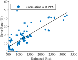
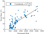
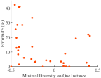
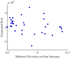
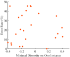
In this subsection, experiments are conducted to verify the proposed relationship between the proposed diversity and generalization performance of classification ensembles (Theorem 2). Before that, we need to verify the ensemble performance’s relationship with the estimated risk. The experimental results are reported in Figure 6, including different individual classifiers. In each experiment, the estimated risk was calculated by Eq. (25), based on the proposed diversity by Eq. (11). The correlation between estimated risk and real error rate was calculated, as annotations shown in Figures 6LABEL:sub@fig:eg1:B-NB-partset:a–6LABEL:sub@fig:eg1:B-LM2-partset:b, presenting a high level of correlation between them. Besides, experimental results reported in Figures 8–8 indicate that the relationship between the proposed diversity and ensemble performance in Theorem 2 is faithful. Along with the increase of diversity, the ensemble performance would show an “upward-downward-upward-downward” trend in Figures 8LABEL:sub@fig:eg3:BagDT:a and 8LABEL:sub@fig:eg3:AdaLM1:a, which coincides with the analyses in Section III-C. Therefore, we could utilize the proposed relationship between the proposed diversity and generalization error to guide our understanding of diversity, and this relationship is a good start to dig the real role of diversity in ensemble learning.

IV-C Comparison Between EPBD and the State-of-the-art Ensemble Pruning Methods

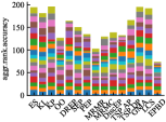
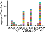
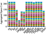
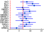
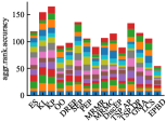
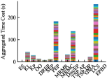
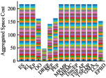
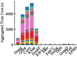
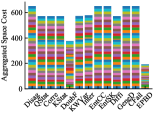
In this subsection, we compare the performance of various ensemble pruning methods, including ES, KL, KP, OO, DREP, SEP, PEP, MRMR, MRMC, DiscEP, TSP.AP, TSP.DP, GMA, and LCS with the proposed EPBD method. Experimental results reported in Tables II–III contain the average test accuracy of each method and the corresponding standard deviation under $5$-fold cross-validation on each data set. For instance, each row (data set) in Table II compares the classification accuracy using bagging with the same type of individual classifiers, indicating results with higher accuracy and lower standard deviation by bold fonts. Besides, the significance of the difference in the accuracy performance between the two methods is examined by two-tailed paired $t$-tests at $5\%$ significance level to tell if two ensemble pruning methods have significantly different results. Two methods end in a tie if there is no significant statistical difference; otherwise, the one with higher values of accuracy will win. The performance of each method is reported in the last two rows of Table II, compared with EPBD in terms of the average rank and the number of data sets that EPBD has won, tied, or lost, respectively. We may notice that OO or PEP might achieve the best results instead of EPBD in a few cases. Yet EPBD could still reach an equal level of accuracy performance without significant difference ending up with a tie. Moreover, both of them cannot restrict the number of classifiers after ensemble pruning like EPBD does, leading to keeping more individual classifiers than we desire in most situations. Meanwhile, it could be inferred that EPBD could achieve competitive results even though it only keeps fewer individual classifiers, which means that the principle we used to guide the pruning process is effective and that utilizing our proposed relationship is reasonable. Figure 10LABEL:sub@fig,expt4sbi:bag,a shows that EPBD could achieve competitive results as OO, PEP, MRMR, and TSP.AP, and EPBD has significant superiority over other compared pruning methods. Figure 10LABEL:sub@fig,expt4sbi:bag,b presents the aggregated rank for each method, describing the similar conclusions to Figure 10LABEL:sub@fig,expt4sbi:bag,a. Figures 10LABEL:sub@fig,expt4sbi:bag,c–10LABEL:sub@fig,expt4sbi:bag,d illustrate the aggregated time cost and the aggregated space cost for each pruning method, respectively. It could be inferred that PEP, DiscEP, and LCS usually cost huge processing time to do ensemble pruning tasks. Similar results are reported in Figure 10.

IV-D Comparison Between EPBD and FTAD Using Other Diversity Measures

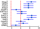
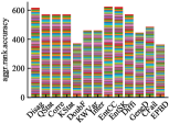
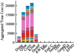
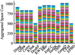
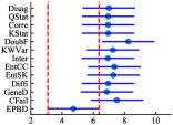
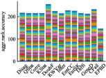
In this subsection, we compare the performance of FTAD with various diversity measures involved, including pairwise measures (Disag, QStat, Corre, KStat, and DoubF) and non-pairwise measures (KWVar, Inter, EntCC, EntSK, Diffi, GeneD, and CFail) with the proposed EPBD method. Experimental results reported in Tables IV–VI contain the average test accuracy of each method and the corresponding standard deviation under $5$-fold cross-validation on each data set. For instance, each row (data set) in Table IV compares the classification accuracy using bagging with the same type of individual classifiers, indicating results with higher accuracy and lower standard deviation by bold fonts. Besides, the significance of the difference in the accuracy performance between two methods is examined by two-tailed paired $t$-tests at $5\%$ significance level to tell if two diversity measures used in FTAD have significantly different results. Two measures end in a tie if there is no significant statistical difference; otherwise, the one with higher values of accuracy will win. The performance of each measure is reported in the last two rows of Table IV, compared with EPBD using the proposed diversity measure in this paper in terms of the average rank and the number of data sets that EPBD has won, tied, or lost, respectively. It could be inferred that EPBD could achieve competitive results with FTAD using other diversity measures according to the results of two-tailed paired $t$-tests in Tables IV–VI. The similar observations also appear in Figures 12–12. Moreover, Figures 12–12 present the time cost and space cost for each diversity measure. It could be inferred that pairwise diversity measures used in FTAD usually cost much more time during the pruning process, as shown in Figure 12LABEL:sub@fig,expt3bi:bag,c and Figure 12LABEL:sub@fig,expt3bi:ada,c.

IV-E Comparison of Space Cost Between EPBD and Methods that Cannot Fix the Size of Pruned Sub-Ensembles

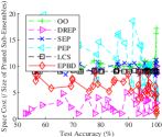
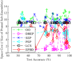
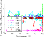
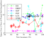
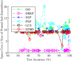
In this subsection, we compare the accuracy and the space cost between EPBD with methods that cannot fix the size of pruned sub-ensembles, such as OO, DREP, SEP, PEP, and LCS. Experimental results are reported in Figure 13. As shown in Figure 13, DREP only keeps one of the individual classifiers that is not an ensemble at all in most cases; OO, SEP, and PEP usually generate pruned sub-ensembles with a larger size than the up limit of that; the size of pruned sub-ensembles generated by LCS is relatively steady around the up limit of that. Besides, although EPBD cannot fix the number of individual classifiers in the pruned sub-ensemble, it could guarantee that the size of the pruned sub-ensemble is no more than the up limit of that, based on the pruning rate. More comparison of space cost could be referred to Figure 10LABEL:sub@fig,expt4sbi:bag,d and Figure 10LABEL:sub@fig,expt4sbi:ada,d. Therefore, we could conclude that EPBD could run as expected to generate a comparable ensemble performance with a smaller size to the original ensemble.

V Conclusion

This paper has investigated and utilized diversity in classification ensembles, and it made the following contributions to the ensemble learning community. First of all, inspired by the regression ensembles, this paper proposed the measure of diversity utilizing the error decomposition for classification ensembles, which broke the error of classification ensembles into two terms: the accuracy and the diversity terms. The empirical results have confirmed that “$\mathop{\rm{div}}$” is a distinct diversity measure. Secondly, we have theoretically investigated the relationship between the proposed diversity and generalization of the ensemble through the bound between margin and generalization. These theoretical analyses solve an open question in the ensemble area to some extent, i.e., when does diversity help the generalization of ensembles? Based on the analyses, the relationship between the proposed diversity and generalization error varies when diversity is in different ranges. In some ranges, more diversity could lead to better generalization, while in other ranges, more diversity is not beneficial to the generalization based on the bound analyses. Thirdly, in order to validate and employ the relationship of diversity to improve the performance of ensembles, we have proposed EPBD that can prune an ensemble without much performance degradation. Besides, an ensemble pruning framework (i.e., FTAD) is proposed to utilize the trade-off between accuracy and diversity and generate pruned sub-ensembles with a smaller size. Note that in FTAD, not only the proposed diversity measure in this paper but also other existing diversity measures could be employed. Although this generalization bound could be loose, our work provides a direction and one theoretical attempt to reveal the impacts of diversity on the generalization. Our future work is to generalize the proposed methodology to the multi-classification problems.

[Example of Extended Analyses in Multi-Classification Problems]

In this section, we give a short example to extend the aforementioned analyses in Section III to multi-classification problems, that means $\mathcal{Y}=\{0,1,...,n_{c}-1\}$ with $n_{c}\,(n_{c}\geqslant 2\,,$  $n_{c}\in\mathbb{Z}^{+})$ different labels. Individual classifiers in an ensemble $(F=\{f_{1},...,f_{|F|}\})$ have been trained and are combined by weighted voting, i.e.,

$$\small f_{ens}(\mathbf{x})=\operatorname*{argmax}_{c_{k}\in\mathcal{Y}}\sum_{i\in[|F|]}w_{i}\mathbb{I}\big{(}f_{i}(\mathbf{x})=c_{k}\big{)}\,,$$ (35)

where $w_{i}$ is the weight corresponding to the individual classifier $f_{i}$, satisfying that $\sum_{i\in[|F|]}w_{i}=1,\,\forall\,w_{i}\geqslant 0$ . To extend the aforementioned analyses in Section III to multi-classification problems, we give the extended proposed error decomposition and diversity measure as a short example. To this end, we need to extend the margin of an ensemble to multi-classification problems first. Inspired by [110], we introduce a new concept named as “credence” of one classifier $f(\cdot)$, represented by $\mathop{\rm{cred}}(\cdot)$, as mappings from $\mathcal{X}\times\mathcal{Y}$ to $[0,1]$, with the interpretation that the result $f(\mathbf{x})$ predicted by $f$ is more plausible for the label $y$ of the instance $\mathbf{x}$ if $\mathop{\rm{cred}}(f,\mathbf{x},y)$ is closer to $1$. Besides, the credence of the ensemble $f_{ens}$ on one instance $(\mathbf{x},y)$ is defined as

$$\small\mathop{\rm{cred}}(f_{ens},\mathbf{x},y)=\sum_{i\in[|F|]}w_{i}\cdot\mathop{\rm{cred}}(f_{i},\mathbf{x},y)\,,$$ (36)

therefore the ensemble predicts label $y$ for the instance $\mathbf{x}$ if $\mathop{\rm{cred}}(f_{ens},\mathbf{x},y)>\max_{y^{\prime}\neq y,\,y^{\prime}\in\mathcal{Y}}\mathop{\rm{cred}}(f_{ens},\mathbf{x},y^{\prime})$ (and ties are broken arbitrarily). Subsequently, the margin of the ensemble on the instance is defined as

$$\small\mathop{\rm{margin}}(f_{ens},\mathbf{x})=\mathop{\rm{cred}}(f_{ens},\mathbf{x},y)-\max_{y^{\prime}\neq y,\,y^{\prime}\in\mathcal{Y}}\mathop{\rm{cred}}(f_{ens},\mathbf{x},y^{\prime})\,,$$ (37)

and that of one individual classifier $f_{i}$ could be obtained similarly. Consequently, $f_{ens}$ would give the wrong prediction on $(\mathbf{x},y)$ only if $\mathop{\rm{margin}}(f_{ens},\mathbf{x})\leqslant 0$. Similar to Section III-A, we define the error function as

$$\small\mathop{\rm{Err}}(f_{ens},\mathbf{x})=\frac{1}{2}\big{(}1-\mathop{\rm{margin}}(f_{ens},\mathbf{x})\big{)}\,,$$ (38)

and the diversity measure would be

$$\small\mathop{\rm{div}}(f_{ens},\mathbf{x})=\sum_{i\in[|F|]}w_{i}\cdot\mathop{\rm{Err}}(f_{i},\mathbf{x})-\mathop{\rm{Err}}(f_{ens},\mathbf{x})\,.$$ (39)

The remaining issue is the definitions of credence. As we know in binary classification problems where $\mathcal{Y}=\{-1,+1\}$, the credence of one classifier $f$ is supposed to be viewed as

$$\small\mathop{\rm{cred}}(f,\mathbf{x},y)=\frac{f(\mathbf{x})y+1}{2}\,.$$ (40)

As for multi-classification problems where $\mathcal{Y}=\{0,1,...,n_{c}-1\}\,(n_{c}\geqslant 2,\,n_{c}\in\mathbb{Z}^{+})$, three functions could be proposed as possible forms of credence, i.e.,

$$\mathop{\rm{cred}}{}_{1}(f,\mathbf{x},y)= \mathbb{I}\big{(}f(\mathbf{x})=y\big{)}\,,$$ (41a)

$$\mathop{\rm{cred}}{}_{2}(f,\mathbf{x},y)= 1-\frac{|f(\mathbf{x})-y|}{n_{c}-1}\,,$$ (41b)

$$\mathop{\rm{cred}}{}_{3}(f,\mathbf{x},y)= 1-\frac{\big{(}f(\mathbf{x})-y\big{)}^{2}}{(n_{c}-1)^{2}}\,.$$ (41c)

Consequently, the difference between the ensemble and its individual members, defined as the “diversity” measure, could be obtained by

$$\mathop{\rm{div}}(f_{ens},\mathbf{x})= -\bigg{(}\mathop{\rm{Err}}(f_{ens},\mathbf{x})-\sum_{i\in[|F|]}w_{i}\cdot\mathop{\rm{Err}}(f_{i},\mathbf{x})\bigg{)}$$

$$= \sum_{i\in[|F|]}w_{i}\cdot\frac{\mathop{\rm{margin}}(f_{ens},\mathbf{x})-\mathop{\rm{margin}}(f_{i},\mathbf{x})}{2}$$

$$= \sum_{i\in[|F|]}w_{i}\cdot\frac{\mathop{\rm{cred}}(f_{ens},\mathbf{x},y)-\mathop{\rm{cred}}(f_{i},\mathbf{x},y)}{2}$$

$$- \sum_{i\in[|F|]}\frac{w_{i}}{2}\bigg{(}\max_{y^{\prime}\neq y}\mathop{\rm{cred}}(f_{ens},\mathbf{x},y^{\prime})-\max_{y^{\prime}\neq y}\mathop{\rm{cred}}(f_{i},\mathbf{x},y^{\prime})\bigg{)},$$ (42)

that is,

$$\mathop{\rm{div}}(f_{ens},\mathbf{x})= \frac{1}{2}\sum_{i\in[|F|]}w_{i}\cdot\max_{y^{\prime}\neq y}\mathop{\rm{cred}}(f_{i},\mathbf{x},y^{\prime})$$

$$- \frac{1}{2}\max_{y^{\prime}\neq y}\mathop{\rm{cred}}(f_{ens},\mathbf{x},y^{\prime})\,.$$ (43)

Analogous results like Theorem 1 could be obtained subsequently. Notice that the appendix is to point out one possibility of extending our theoretical results to multi-classification problems, which is a start. Further investigations and careful experiments are still needed before getting a more promising conclusion.

References

- [1] Z.-H. Zhou, Ensemble Methods: Foundations and Algorithms. CRC press, 2012.
- [2] R. Girshick, J. Donahue, T. Darrell, and J. Malik, “Rich feature hierarchies for accurate object detection and semantic segmentation,” in CVPR, 2014, pp. 580–587.
- [3] J. Wang, Z. Liu, Y. Wu, and J. Yuan, “Mining actionlet ensemble for action recognition with depth cameras,” in CVPR, 2012, pp. 1290–1297.
- [4] X. Zhou, L. Xie, P. Zhang, and Y. Zhang, “An ensemble of deep neural networks for object tracking,” in ICIP, Oct 2014, pp. 843–847.
- [5] H. Ykhlef and D. Bouchaffra, “An efficient ensemble pruning approach based on simple coalitional games,” Inform Fusion, vol. 34, pp. 28–42, 2017.
- [6] J. Sun, L. Li, and Q. Hu, “Fault diagnosis based on pruned ensemble,” in ICMLC, vol. 1, 2012, pp. 35–40.
- [7] J. H. Abawajy, M. Chowdhury, and A. Kelarev, “Hybrid consensus pruning of ensemble classifiers for big data malware detection,” IEEE T Cloud Comput, vol. 8, no. 2, pp. 398–407, 2020.
- [8] Z. Liu, C. Li, X. Gao, G. Wang, and J. Yang, “Ensemble-based depression detection in speech,” in IEEE BIBM, 2017, pp. 975–980.
- [9] R. Diao, F. Chao, T. Peng, N. Snooke, and Q. Shen, “Feature selection inspired classifier ensemble reduction,” IEEE T Cybernetics, vol. 44, no. 8, pp. 1259–1268, 2014.
- [10] Z. Sun, Q. Song, and X. Zhu, “Using coding-based ensemble learning to improve software defect prediction,” IEEE T Syst Man Cy C, vol. 42, no. 6, pp. 1806–1817, 2012.
- [11] W.-Y. Lin, Y.-H. Hu, and C.-F. Tsai, “Machine learning in financial crisis prediction: A survey,” IEEE T Syst Man Cy C, vol. 42, no. 4, pp. 421–436, 2012.
- [12] A. Dutta and P. Dasgupta, “Ensemble learning with weak classifiers for fast and reliable unknown terrain classification using mobile robots,” IEEE T Syst Man Cy-S, vol. 47, no. 11, pp. 2933–2944, 2017.
- [13] D. Guo, Y. Jin, J. Ding, and T. Chai, “Heterogeneous ensemble-based infill criterion for evolutionary multiobjective optimization of expensive problems,” IEEE T Cybernetics, vol. 49, no. 3, pp. 1012–1025, 2019.
- [14] Y. Bi, B. Xue, and M. Zhang, “Genetic programming with a new representation to automatically learn features and evolve ensembles for image classification,” IEEE T Cybernetics, pp. 1–15, 2020.
- [15] J. Zhuang, K. Geng, and G. Yin, “Ensemble learning based brain-computer interface system for ground vehicle control,” IEEE T Syst Man Cy-S, pp. 1–13, 2019.
- [16] R. Cheng, W. Yu, Y. Song, D. Chen, X. Ma, and Y. Cheng, “Intelligent safe driving methods based on hybrid automata and ensemble cart algorithms for multihigh-speed trains,” IEEE T Cybernetics, vol. 49, no. 10, pp. 3816–3826, 2019.
- [17] N. Liu, H. Wu, and L. Lin, “Hierarchical ensemble of background models for ptz-based video surveillance,” IEEE T Cybernetics, vol. 45, no. 1, pp. 89–102, 2015.
- [18] F. Xiong, Y. Xiao, Z. Cao, Y. Wang, J. T. Zhou, and J. Wu, “Ecml: An ensemble cascade metric-learning mechanism toward face verification,” IEEE T Cybernetics, pp. 1–14, 2020.
- [19] H. Song, D. Ding, H. Dong, and Q.-L. Han, “Distributed maximum correntropy filtering for stochastic nonlinear systems under deception attacks,” IEEE T Cybernetics, pp. 1–12, 2020.
- [20] X. Wu, V. Kumar, J. R. Quinlan, J. Ghosh, Q. Yang, H. Motoda, G. J. McLachlan, A. Ng, B. Liu, S. Y. Philip et al., “Top 10 algorithms in data mining,” Knowl Inf Syst, vol. 14, no. 1, pp. 1–37, 2008.
- [21] L. Rokach, “Ensemble-based classifiers,” Artif Intell Rev, vol. 33, no. 1-2, pp. 1–39, 2010.
- [22] F. Herrera, F. Charte, A. J. Rivera, and M. J. del Jesus, “Ensemble-based classifiers,” in Multilabel Classification. Springer, 2016, pp. 101–113.
- [23] S. Gu, R. Cheng, and Y. Jin, “Multi-objective ensemble generation,” Wires Data Min Knowl, vol. 5, no. 5, pp. 234–245, 2015.
- [24] T. Dietterich, “Ensemble methods in machine learning,” in MCS, vol. 1857, 2000, pp. 1–15.
- [25] Z. Lu, X. Wu, X. Zhu, and J. Bongard, “Ensemble pruning via individual contribution ordering,” in SIGKDD. ACM, 2010, pp. 871–880.
- [26] E. Tang, P. Suganthan, and X. Yao, “An analysis of diversity measures,” Mach Learn, vol. 65, no. 1, pp. 247–271, jul 2006.
- [27] A. Tsymbal, M. Pechenizkiy, and P. Cunningham, “Diversity in search strategies for ensemble feature selection,” Inform Fusion, vol. 6, no. 1, pp. 83–98, 2005.
- [28] L. Kuncheva and C. Whitaker, “Measures of diversity in classifier ensembles and their relationship with the ensemble accuracy,” Mach Learn, vol. 51, no. 2, pp. 181–207, 2003.
- [29] G. Brown, “An information theoretic perspective on multiple classifier systems,” in MCS, 2009, pp. 344–353.
- [30] Z.-H. Zhou and N. Li, “Multi-information ensemble diversity,” in MCS, 2010, pp. 134–144.
- [31] Y. Yu, Y.-F. Li, and Z.-H. Zhou, “Diversity regularized machine,” in IJCAI, 2011, p. 1603.
- [32] Z. Jiang, H. Liu, B. Fu, and Z. Wu, “Generalized ambiguity decompositions for classification with applications in active learning and unsupervised ensemble pruning.” in AAAI, 2017, pp. 2073–2079.
- [33] A. Krogh and J. Vedelsby, “Neural network ensembles, cross validation, and active learning,” in NIPS, 1995, pp. 231–238.
- [34] S. Geman, E. Bienenstock, and R. Doursat, “Neural networks and the bias/variance dilemma,” Neural Comput, vol. 4, no. 1, pp. 1–58, 1992.
- [35] N. Li, Y. Yu, and Z.-H. Zhou, “Diversity regularized ensemble pruning,” in ECML-PKDD, 2012, pp. 330–345.
- [36] R. Herbrich and T. Graepel, “A pac-bayesian margin bound for linear classifiers: Why svms work,” in NIPS, 2001, pp. 224–230.
- [37] ——, “A pac-bayesian margin bound for linear classifiers,” IEEE T Inform Theory, vol. 48, no. 12, pp. 3140–3150, 2002.
- [38] L. Breiman, “Bagging predictors,” Mach Learn, vol. 24, no. 2, pp. 123–140, 1996.
- [39] Y. Freund and R. Schapire, “A desicion-theoretic generalization of on-line learning and an application to boosting,” in EuroCOLT. Springer, 1995, pp. 23–37.
- [40] ——, “A decision-theoretic generalization of on-line learning and an application to boosting,” J Comput Syst Sci, vol. 55, no. 1, pp. 119–139, 1997.
- [41] Y. Freund, R. E. Schapire et al., “Experiments with a new boosting algorithm,” in ICML, vol. 96. Bari, Italy, 1996, pp. 148–156.
- [42] L. Breiman, “Random forests,” Mach Learn, vol. 45, no. 1, pp. 5–32, 2001.
- [43] J. J. Rodriguez, L. I. Kuncheva, and C. J. Alonso, “Rotation forest: A new classifier ensemble method,” IEEE T Pattern Anal, vol. 28, no. 10, pp. 1619–1630, 2006.
- [44] A. Chandra and X. Yao, “Divace: Diverse and accurate ensemble learning algorithm,” in IDEAL. Springer, 2004, pp. 619–625.
- [45] F. Roli, G. Giacinto, and G. Vernazza, “Methods for designing multiple classifier systems,” in MCS. Springer, 2001, pp. 78–87.
- [46] S. Gu and Y. Jin, “Generating diverse and accurate classifier ensembles using multi-objective optimization,” in MCDM. IEEE, 2014, pp. 9–15.
- [47] G. U. Yule, “On the association of attributes in statistics: with illustrations from the material of the childhood society, &c,” Phil. Trans. R. Soc. Lond. A, vol. 194, no. 252-261, pp. 257–319, 1900.
- [48] J. Cohen, “A coefficient of agreement for nominal scales,” Educ Psychol Meas, vol. 20, no. 1, pp. 37–46, 1960.
- [49] D. B. Skalak et al., “The sources of increased accuracy for two proposed boosting algorithms,” in AAAI, vol. 1129, 1996, p. 1133.
- [50] T. K. Ho, “The random subspace method for constructing decision forests,” IEEE T Pattern Anal, vol. 20, no. 8, pp. 832–844, 1998.
- [51] P. Sneath and R. Sokal, Numerical taxonomy: The principles and practice of numerical classification. WH Freeman, 1973.
- [52] G. Giacinto and F. Roli, “Design of effective neural network ensembles for image classification purposes,” Image Vision Comput, vol. 19, no. 9, pp. 699–707, 2001.
- [53] J. L. Fleiss, B. Levin, and M. C. Paik, Statistical methods for rates and proportions. John Wiley & Sons, 2013.
- [54] R. Kohavi, D. H. Wolpert et al., “Bias plus variance decomposition for zero-one loss functions,” in ICML, vol. 96, 1996, pp. 275–83.
- [55] P. Cunningham and J. Carney, “Diversity versus quality in classification ensembles based on feature selection,” in ECML. Springer, 2000, pp. 109–116.
- [56] C. A. Shipp and L. I. Kuncheva, “Relationships between combination methods and measures of diversity in combining classifiers,” Inform Fusion, vol. 3, no. 2, pp. 135–148, 2002.
- [57] L. K. Hansen and P. Salamon, “Neural network ensembles,” IEEE T Pattern Anal, vol. 12, no. 10, pp. 993–1001, 1990.
- [58] D. Partridge and W. Krzanowski, “Software diversity: practical statistics for its measurement and exploitation,” Inform Software Tech, vol. 39, no. 10, pp. 707–717, 1997.
- [59] Y. Liu and X. Yao, “Ensemble learning via negative correlation,” Neural Networks, vol. 12, no. 10, pp. 1399–1404, 1999.
- [60] H. Chen and X. Yao, “Multiobjective neural network ensembles based on regularized negative correlation learning,” IEEE T Knowl Data En, vol. 22, no. 12, pp. 1738–1751, 2010.
- [61] G. Zenobi and P. Cunningham, “Using diversity in preparing ensembles of classifiers based on different feature subsets to minimize generalization error,” in ECML. Springer, 2001, pp. 576–587.
- [62] Z. Liu, Q. Dai, and N. Liu, “Ensemble selection by grasp,” Appl Intell, vol. 41, no. 1, pp. 128–144, 2014.
- [63] Y. Kokkinos and K. G. Margaritis, “Confidence ratio affinity propagation in ensemble selection of neural network classifiers for distributed privacy-preserving data mining,” Neurocomputing, vol. 150, pp. 513–528, 2015.
- [64] C.-X. Zhang, J.-S. Zhang, and Q.-Y. Yin, “A ranking-based strategy to prune variable selection ensembles,” Knowl-Based Syst, vol. 125, pp. 13–25, 2017.
- [65] R. Lysiak, M. Kurzynski, and T. Woloszynski, “Optimal selection of ensemble classifiers using measures of competence and diversity of base classifiers,” Neurocomputing, vol. 126, pp. 29–35, 2014.
- [66] I. Partalas, G. Tsoumakas, and I. P. Vlahavas, “Focused ensemble selection: A diversity-based method for greedy ensemble selection.” in ECAI, 2008, pp. 117–121.
- [67] R. Caruana, A. Niculescu-Mizil, G. Crew, and A. Ksikes, “Ensemble selection from libraries of models,” in ICML. ACM, 2004, p. 18.
- [68] R. E. Banfield, L. O. Hall, K. W. Bowyer, and W. P. Kegelmeyer, “Ensemble diversity measures and their application to thinning,” Inform Fusion, vol. 6, no. 1, pp. 49–62, 2005.
- [69] D. Margineantu and T. Dietterich, “Pruning adaptive boosting,” in ICML, vol. 97, 1997, pp. 211–218.
- [70] Z.-H. Zhou, J. Wu, and W. Tang, “Ensembling neural networks: many could be better than all,” Artif Intell, vol. 137, no. 1-2, pp. 239–263, 2002.
- [71] G. Martínez-Muñoz and A. Suárez, “Using boosting to prune bagging ensembles,” Pattern Recogn Lett, vol. 28, no. 1, pp. 156–165, 2007.
- [72] G. Tsoumakas, I. Partalas, and I. Vlahavas, “An ensemble pruning primer,” in SUEMA. Springer, 2009, pp. 1–13.
- [73] H. Zhang, Y. Song, B. Jiang, B. Chen, and G. Shan, “Two-stage bagging pruning for reducing the ensemble size and improving the classification performance,” Math Probl Eng, vol. 2019, 2019.
- [74] M. A. O. Ahmed, L. Didaci, B. Lavi, and G. Fumera, “Using diversity for classifier ensemble pruning: An empirical investigation,” TAAI, vol. 29, no. 1-2, pp. 25–39, 2017.
- [75] X. Zeng, D. F. Wong, and L. S. Chao, “Constructing better classifier ensemble based on weighted accuracy and diversity measure,” The Scientific World Journal, vol. 2014, 2014.
- [76] G. Tsoumakas, I. Katakis, and I. Vlahavas, “Effective voting of heterogeneous classifiers,” in ECML. Springer, 2004, pp. 465–476.
- [77] G. D. Cavalcanti, L. S. Oliveira, T. J. Moura, and G. V. Carvalho, “Combining diversity measures for ensemble pruning,” Pattern Recogn Lett, vol. 74, pp. 38–45, 2016.
- [78] Z.-H. Zhou and W. Tang, “Selective ensemble of decision trees,” in RSFDGrC, 2003, pp. 476–483.
- [79] I. Partalas, G. Tsoumakas, and I. Vlahavas, “A study on greedy algorithms for ensemble pruning,” Dept. of Informatics, Aristotle University of Thessaloniki, Greece, Tech. Rep. TR-LPIS-360-12, LPIS, 2012.
- [80] H. Guo, F. Sun, J. Cheng, Y. Li, and M. Xu, “A novel margin-based measure for directed hill climbing ensemble pruning,” Math Probl Eng, vol. 2016, pp. 1–11, 2016.
- [81] C. Qian, Y. Yu, and Z.-H. Zhou, “Pareto ensemble pruning,” in AAAI, 2015, pp. 2935–2941.
- [82] X. Xia, T. Lin, and Z. Chen, “Maximum relevancy maximum complementary based ordered aggregation for ensemble pruning,” Appl Intell, vol. 48, no. 9, pp. 2568–2579, 2018.
- [83] J. Cao, W. Li, C. Ma, and Z. Tao, “Optimizing multi-sensor deployment via ensemble pruning for wearable activity recognition,” Inform Fusion, vol. 41, pp. 68–79, 2018.
- [84] V. Soto, S. García-Moratilla, G. Martínez-Muñoz, D. Hernández-Lobato, and A. Suárez, “A double pruning scheme for boosting ensembles,” IEEE T Cybernetics, vol. 44, no. 12, pp. 2682–2695, 2014.
- [85] Y. Zhang, S. Burer, and W. N. Street, “Ensemble pruning via semi-definite programming,” J Mach Learn Res, vol. 7, no. Jul, pp. 1315–1338, 2006.
- [86] G. Martínez-Muñoz, D. Hernández-Lobato, and A. Suárez, “An analysis of ensemble pruning techniques based on ordered aggregation,” IEEE T Pattern Anal, vol. 31, no. 2, pp. 245–259, 2009.
- [87] G. Martınez-Munoz and A. Suárez, “Aggregation ordering in bagging,” in AIA. Citeseer, 2004, pp. 258–263.
- [88] I. Partalas, G. Tsoumakas, and I. Vlahavas, “An ensemble uncertainty aware measure for directed hill climbing ensemble pruning,” Mach Learn, vol. 81, no. 3, pp. 257–282, 2010.
- [89] D. Hernandez-Lobato, G. Martinez-Munoz, and A. Suarez, “Statistical instance-based pruning in ensembles of independent classifiers,” IEEE T Pattern Anal, vol. 31, no. 2, pp. 364–369, 2009.
- [90] G. Martinez-munoz, D. Hernandez-lobato, and A. Suarez, “Statistical instance-based ensemble pruning for multi-class problems,” in ICANN. Springer Berlin Heidelberg, 2009, pp. 90–99.
- [91] J. Cao, W. Yuan, W. Li, and E. Xiaozheng, “Dynamic ensemble pruning selection using meta-learning for multi-sensor based activity recognition,” in SmartWorld/SCALCOM/UIC/ATC/CBDCom/IOP/SCI, August 2019, pp. 1063–1068.
- [92] D. Hernandez-Lobato, G. Martinez-Munoz, and A. Suarez, “Inference on the prediction of ensembles of infinite size,” Pattern Recogn, vol. 44, no. 7, pp. 1426–1434, 2011.
- [93] W. Fan, F. Chu, H. Wang, and P. S. Yu, “Pruning and dynamic scheduling of cost-sensitive ensembles,” in AAAI, 2002, pp. 146–151.
- [94] H. Wang, W. Fan, P. S. Yu, and J. Han, “Mining concept-drifting data streams using ensemble classifiers,” in SIGKDD, August 2003, pp. 226–235.
- [95] J. D. Basilico, M. A. Munson, T. G. Kolda, K. R. Dixon, and W. P. Kegelmeyer, “Comet: A recipe for learning and using large ensembles on massive data,” in ICDM, 2011, pp. 41–50.
- [96] Z. Jiang, H. Liu, B. Fu, and Z. Wu, “A novel bayesian ensemble pruning method,” in ICDM Workshops, 2016, pp. 1205–1212.
- [97] B. Krawczyk and M. Wozniak, “Experiments on simultaneous combination rule training and ensemble pruning algorithm,” in CIEL, 2014, pp. 1–6.
- [98] L. G. Valiant, “A theory of the learnable,” Commun ACM, vol. 27, no. 11, pp. 1134–1142, 1984.
- [99] G. Brown, J. L. Wyatt, and P. Tiňo, “Managing diversity in regression ensembles,” J Mach Learn Res, vol. 6, no. Sep, pp. 1621–1650, 2005.
- [100] J. Mendes-Moreira, C. Soares, A. M. Jorge, and J. F. D. Sousa, “Ensemble approaches for regression: A survey,” ACM Comput Surv, vol. 45, no. 1, p. 10, 2012.
- [101] D. M. Department, “The first and second derivatives,” Website, accessed on October 26, 2019. [Online]. Available: https://math.dartmouth.edu/opencalc2/cole/lecture8.pdf
- [102] J. Demšar, “Statistical comparisons of classifiers over multiple data sets,” J Mach Learn Res, vol. 7, no. Jan, pp. 1–30, 2006.
- [103] M. Lichman, “UCI machine learning repository,” 2013. [Online]. Available: http://archive.ics.uci.edu/ml
- [104] Y. Freund, “Boosting a weak learning algorithm by majority,” Inform Comput, vol. 121, no. 2, pp. 256–285, 1995.
- [105] Martínez-Muñoz and Suárez, “Pruning in ordered bagging ensembles,” in ICML, 2006, pp. 609–616.
- [106] S. Aghamolaei, M. Farhadi, and H. Zarrabi-Zadeh, “Diversity maximization via composable coresets,” in CCCG, 2015, p. 43.
- [107] P. Indyk, S. Mahabadi, M. Mahdian, and V. Mirrokni, “Composable core-sets for diversity and coverage maximization,” in PODS, 2014, pp. 100–108.
- [108] Wikipedia, “Correlation coefficient,” Website, accessed on November 2, 2020. [Online]. Available: https://en.wikipedia.org/wiki/Correlation_coefficient
- [109] ——, “Pearson correlation coefficient,” Website, accessed on November 2, 2020. [Online]. Available: https://en.wikipedia.org/wiki/Pearson_correlation_coefficient
- [110] R. Schapire, Y. Freund, P. Bartlett, W. Lee et al., “Boosting the margin: A new explanation for the effectiveness of voting methods,” Ann Stat, vol. 26, no. 5, pp. 1651–1686, 1998.