Continuous Control with Contexts, Provably

Abstract

A fundamental challenge in artificial intelligence is to build an agent that generalizes and adapts to unseen environments. A common strategy is to build a decoder that takes the context of the unseen new environment as input and generates a policy accordingly. The current paper studies how to build a decoder for the fundamental continuous control task, linear quadratic regulator (LQR), which can model a wide range of real-world physical environments. We present a simple algorithm for this problem, which uses upper confidence bound (UCB) to refine the estimate of the decoder and balance the exploration-exploitation trade-off. Theoretically, our algorithm enjoys a $\widetilde{O}\left(\sqrt{T}\right)$ regret bound in the online setting where $T$ is the number of environments the agent played. This also implies after playing $\widetilde{O}\left(1/\epsilon^{2}\right)$ environments, the agent is able to transfer the learned knowledge to obtain an $\epsilon$-suboptimal policy for an unseen environment. To our knowledge, this is first provably efficient algorithm to build a decoder in the continuous control setting. While our main focus is theoretical, we also present experiments that demonstrate the effectiveness of our algorithm.

1 Introduction

Humans are able to solve a new task without any training based on previous experience in similar tasks. The desired intelligent agent should be able do the same, learning from previous experience, adapting to the new ones and improving the performance as the agent gains more experience. This is a challenging problem as we need to design an adaptation mechanism which is fundamentally different from classical supervised learning methods.

A common approach is to build a decoder so that once the agent sees a description of new task, i.e., the context of the new task, the decoder turns the context into a succinct representation of the new task, based on which the agent is able to design a policy to solve the task. Note this procedure resembles how a human solves a new task. For example, if a human wants to push an object on a table, the human first sees the object and the table (context). Then, in his/her mind, the context becomes a representation of this task, e.g., a sense of weight of the object. Based on this representation, the human can easily reason about how much force to exert on the object.

This general approach has been applied in practice. For example, Wu et al. (2018) studied the visual navigation task and built a Bayesian model that takes the context of new environments and outputs the policy that enables the agent to navigate. Killian et al. (2016) used this approach to develop personalized medicine policies for HIV treatment.

While this is a promising approach, currently we only have limited theoretical understanding. The approach can be formulated in Contextual Markov Decision Process (CMDP) framework (Hallak et al., 2015). Recently, there is a line of work gave provable guarantees for CMDP (Abbasi-Yadkori and Neu, 2014; Hallak et al., 2015; Dann et al., 2018; Modi et al., 2018; Modi and Tewari, 2019). These work all study tabular MDPs, and use function approximation, e.g., linear functions, generalized linear models, etc, to model the mapping from the context to the probability transition matrix. A major drawback of these work is that they are restricted to the tabular setting and thus can only deal with discrete environments. Therefore, they can hardly model real-world continuous control tasks, like the task of pushsing an object as we described above. A natural question arises:

Can we design a provably efficient decoder for continuous control problems?

In this paper, we make an important step towards answering this question. We study the fundamental task in continuous control, linear quadratic regulator (LQR). LQR is arguably the most widely used framework in continuous control, as LQR easily models real-world physical phenomena, e.g., the pushing object task we described earlier. We propose a new algorithm that builds a decoder, so that for a new LQR task, the decoder takes LQR’s context and outputs a representation based on which the agent can infer a near-optimal policy for new continuous control tasks. In the training phase, we build the decoder via a sequence of LQRs (in an online fashion) with unknown parameters. For each new task, we first use the current decoder to build the representation of this task, infer a policy based on this representation and use this policy to do control for this episode. There are two crucial components in our algorithm. First, after each episode, we will refine the estimate of the decoder based on the observations from this episode. Second, it is crucial to use a upper confidence bound (UCB) estimator of the decoder to build the representation so that the agent can perform a near-optimal trade-off between exploration and exploitation. In this way, we provably show the decoder improves the performance as it experiences more training tasks. Formally, we show our algorithm enjoys $\widetilde{O}\left(\sqrt{T}\right)$ regret (the difference between the cumulative rewards of our algorithm and the unknown optimal policy on every seen environment) bound in the online setting. Moreover, the algorithm is able to obtain an $\epsilon$-suboptimal policy for an unseen LQR environment after playing $\widetilde{O}\left(\epsilon^{-2}\right)$ environments. To our knowledge, this is the first provably efficient algorithm that builds a decoder for continuous control environments. Empirically, we simulate several physical environments to illustrate the effectiveness of our algorithm.

Organization

This paper is organized as follows. In Section 2, we discuss related work. In Section 3, we formally describe the problem setup. In Section 4, we present our algorithm and its theoretical guarantees. In Section 5, we use simulation on physical environments to demonstrate the effectiveness of our approach. We conclude in Section 6 and defer most technical proofs to the appendix.

2 Related Work

Recently there is a large body of literature focusing on learning for control in LQR systems. The first work we are aware of is Fiechter (1997) which studies the sample complexity of LQR in the offline setting. For the online setting, where the agent can only obtain the next state starting from the present state, the first near-optimal regret bound ($\widetilde{O}(\sqrt{T})$) is due to Abbasi-Yadkori and Szepesvári (2011), which studies the learning problem in the infinite-horizon average-case cost setting. Later on, a sequence of papers (Tu and Recht, 2017; Dean et al., 2017, 2018; Tu and Recht, 2018; Abbasi-Yadkori et al., 2018; Cohen et al., 2019) studied this problem in similar settings, improved efficiency of the algorithms and characterized the gap between model-free and model-based approaches.

Building an agent that quickly adapts to new environment has received increasing interest in the machine learning community. Taylor and Stone (2009) gave a summary for the literature before 2009. More recently, a sequence of theory papers Lehnert and Littman (2018); Spector and Belongie (2018); Abel et al. (2018); Lehnert et al. (2019) studied the transferability of reward knowledge, state-abstraction, and model features for Markov decision processes. Please also refer to references therein for more details. There are also some experimental works, e.g., Santara et al. (2019); Yu et al. (2018); Wu et al. (2018); Gamrian and Goldberg (2018), studying how to transfer knowledge from seen tasks to unseen tasks. Nevertheless, we are not aware of any study on how to provably perform continuous control with contexts.

3 Preliminaries

Notations.

We begin by introducing necessary notations. We write $[h]$ to denote the set $\left\{1,\ldots,h\right\}$. We use $I_{d}\in\mathbb{R}^{d\times d}$ to denote the $d\times d$ identity matrix. We use $0_{d\times d^{\prime}}$ to represent the all-zero matrix in $\mathbb{R}^{d\times d^{\prime}}$. If it is clear from the context, we omit the subscript $d\times d^{\prime}$. Let $\left\|\cdot\right\|_{2}$ denote the Euclidean norm of a vector in $\mathbb{R}^{d}$. For a symmetric matrix $A$, let $\left\|A\right\|_{\mathrm{op}}$ denote its operator norm and $\lambda_{i}\left(A\right)$ denote its $i$-th eigenvalue. Throughout the paper, all sets are multisets, i.e., a single element can appear multiple times.

Finite Horizon Linear Quadratic Regulator.

We now formally define the finite horizon Linear Quadratic Regulator (LQR) problem. In the LQR problem, there is a state space $\mathcal{X}\subset\mathbb{R}^{d}$ and a closed action space $\mathcal{U}\subset\mathbb{R}^{d^{\prime}}$. Suppose we always start from the initial state $x_{1}=x_{\mathrm{init}}\in\mathcal{X}$ and play for $H$ steps. Then at a state $x_{h}\in\mathcal{X}$, if an action $u_{h}\in\mathcal{U}$ is played, the next state is given by

$$x_{h+1}=Ax_{h}+Bu_{h}+w_{h+1},$$ (1)

where $A,B$ are matrices of proper dimension and $w_{h+1}$ is a zero-mean random vector. Here $A,B$ can be viewed as the succinct representation of this LQR since as will be explained below, given $A,B$, one can easily infer the optimal policy for this LQR. For simplicity, we denote

$$M=[A,B],\text{ and }y_{h}=[x_{h}^{\top},u_{h}^{\top}]^{\top}\in\mathbb{R}^{d+d^{\prime}}.$$

Now the state transition can be rewritten as $x_{h+1}=My_{h}+w_{h+1}.$ For the ease of presentation, we assume that the covariance matrix of noise vector $w_{h+1}$ is $\mathbb{E}(w_{h+1}w_{h+1}^{\top})=I_{d}$. Our analysis follows similarly if the covariance matrix is not $I_{d}$ (see e.g. Remark 3 in Abbasi-Yadkori and Szepesvári (2011)). After each step, the player receives an immediate cost $x_{h}^{\top}Q_{h}x_{h}+u_{h}^{\top}R_{h}u_{h},$ where $Q_{h},R_{h}$ are positive definite matrices of proper dimensions. At a terminal state $x_{H}$, there is no action to be played, and the player receives a terminal cost $x_{H}^{\top}Q_{H}x_{H},$ where $Q_{H}$ is a positive semi-definite matrix of proper dimension. The goal of the player is to find a policy $\pi:(\mathcal{X}\times\mathcal{U})^{*}\times\mathcal{X}\rightarrow\mathcal{U}$, which is a function that maps the trajectory $\{(x_{i},u_{i})\}_{i=1}^{h-1}\cup\{x_{h}\}$ to the next action $u_{h}$, such that the following objectives are minimized:

$$\bigg{\{}J^{\pi}_{h}(M,x):=\mathbb{E}\bigg{[}\bigg{(}\sum_{h^{\prime}=h}^{H-1}x_{h}^{\top}Q_{h}x_{h}+u_{h}^{\top}R_{h}u_{h}\bigg{)}+x_{H}^{\top}Q_{f}x_{H}~{}\bigg{|}~{}x_{h}=x\bigg{]}\bigg{\}}_{h\in[H]},$$

where the action $u_{h}$ is given by $u_{h}=\pi[(x_{1},u_{1}),(x_{2},u_{2}),\ldots,(x_{h-1},u_{h-1}),x_{h}]$, and the expectation is over the randomness of $w_{h}$ and $\pi$.

It is well-known that the optimal policy $\pi^{*}$ is Markovian Puterman (2014), i.e., it only depends on the present state. For an unconstrained action space $\mathcal{U}$, we have

$$\forall x\in\mathcal{X},h\in[H-1]:\quad\pi_{h}^{*}(M,x):=K_{h}(M)x$$

where $M=[A,B]$ and $K_{h}(M)$ is a matrix that will be defined shortly. It is also known (see e.g. Bertsekas (1996)) that the optimal cost function $J^{*}_{h}(x):=J^{\pi^{*}}_{h}(x)$ is given by

$$J^{*}_{h}(M,x):=x^{\top}P_{h}(M)x+C_{h}(M)=\inf_{\pi}J_{h}^{\pi}(M,x)$$ (2)

where

$$P_{h}(M)=\begin{cases}Q_{h}+A^{\top}P_{h+1}(M)A-A^{\top}P_{h+1}B(R_{h}+B^{\top}P_{h+1}(M)B)^{-1}B^{\top}P_{h+1}(M)A&h<H\\ Q_{H}&h=H\end{cases}$$ (3)

and

$$C_{h}(M)=\begin{cases}C_{h+1}(M)+\mathbb{E}_{w_{h+1}}\big{[}w_{h+1}^{\top}P_{h+1}(M)w_{h+1}]&h<H\\ 0&h=H\end{cases}.$$

We now define $K_{h}(M)$ as

$$K_{h}(M):=-(R_{h}+B^{\top}P_{h+1}(M)B)^{-1}B^{\top}P_{h+1}(M)A.$$ (4)

Note that the optimal value Equation (2) satisfies Bellman equations,

$$\forall h\in[H-1]:\quad J_{h}^{*}(M,x)=x^{\top}Q_{h}x+{\pi^{*}(x)}^{\top}R_{h}\pi^{*}(x)+\mathbb{E}\big{[}J_{h+1}^{*}(Ax+B\pi^{*}(x)+w)\big{]}$$

and

$$\forall h\in[H-1]:\quad J_{h}^{*}(M,x)=x^{\top}Q_{h}x+\min_{u}\mathbb{E}[u^{\top}R_{h}u+J_{h+1}^{*}(Ax+Bu+w)].$$

Now we have shown that if we are given $A$ and $B$, then we can obtain the optimal policy directly. In this paper, we deal with setting where $A$ and $B$ are unknown and we need to use decoder to decode $A$ and $B$ from the contexts of the current LQR, as specified below.

Learning to Control LQR with Contexts

In the continuous control with contexts setting, in each episode we observe a context

$$(C,D)\sim\mu,$$

where $\mu$ is a distribution on $\mathbb{R}^{p\times d}\times\mathbb{R}^{p^{\prime}\times d^{\prime}}$. The context $[C,D]$ encodes the information of the environment. Formally, the representation ($[A,B]$) of this environment can be decoded from the context via a decoding matrix $\Theta_{*}\in\mathbb{R}^{d\times(p+p^{\prime})}$:

$$[A,B]=\Theta_{*}\cdot\bigg{[}\begin{array}[]{cc}C&0_{p\times d^{\prime}}\\ 0_{p^{\prime}\times d}&D\end{array}\bigg{]}.$$ (7)

From now on, to emphasize that the representation of LQR can be decoded from $\Theta_{*}$, we write

$$M_{\Theta_{*},C,D}:=\Theta_{*}\cdot\bigg{[}\begin{array}[]{cc}C&0_{p\times d^{\prime}}\\ 0_{p^{\prime}\times d}&D\end{array}\bigg{]}=[A,B].$$ (10)

If it is clear from the context, we ignore $[C,D]$ for notational simplicity. Note the optimal decoder $\Theta_{*}$ is unknown to the agent and the goal is to learn $\Theta_{*}$ from contexts and interactions with the environment. Below we formally define the problem that we study.

Definition 3.1 (Contextual Transfer Learning Problem).

Build an agent that plays on $K$ LQR games (one trajectory per game) with context pairs $\{(C^{(1)},D^{(1)}),(C^{(2)},D^{(2)}),\ldots,(C^{(K)},D^{(K)})\}\sim\mu$, for some integer $K\geq 0$ such that for another new context pair $(C,D)\sim\mu$, the agent outputs a policy $\pi$ based on $(C,D)$ which satisfies

$$\mathbb{E}[J^{\pi}_{h}(M_{\Theta_{*},C,D},~{}x_{1})-J^{*}_{h}(M_{\Theta_{*},C,D},~{}x_{1})]\leq\epsilon$$

for some given target accuracy $\epsilon>0$.

Here $K$ is the sample complexity which ideally scales polynomially with $1/\epsilon$ and problem-dependent parameters. The performance of the agent can also be measured by regret, as defined below.

$$\mathrm{Regret}(KH):=\sum_{k=1}^{K}J_{1}^{\widetilde{\pi}^{(k)}}\Big{(}M_{\Theta_{*},C^{(k)},D^{(k)}},~{}x_{1}\Big{)}-J_{1}^{*}\Big{(}M_{\Theta_{*},C^{(k)},D^{(k)}},x_{1}\Big{)},$$ (11)

where $\widetilde{\pi}^{(k)}$ is the policy played at episode $k$ by the agent. This quantity measurse the sub-optimality of policies the agent played in the first $K$ episodes.

Remark 3.1.

We consider matrix-type linear maps from context to the representation only for sake of presentation. Our algorithm and analysis can be readily extended to other linear maps, e.g., $[A_{*}(C),B_{*}(D)]:=f(C,D)$ for some unknown linear function $f$.

4 Main Algorithm

In this section, we first describe the algorithm and then present its sample complexity guarantees.

Algorithm

We describe the high-level idea of the algorithm below. The agent maintains a decoder that maps the context $(C,D)$ to the representation $(A,B)$. We denote $\Theta^{(k)}$ the decoder at the $k$-th episode. Initially, we know nothing about $\Theta_{*}$, so we initialize our decoder by setting $\Theta^{(1)}=0\in\mathbb{R}^{d\times p}$. At the $k$-th episode, the agent plays policy $\pi^{(k)}$ and in each time step $h\in[H-1]$, it collects data

$$x^{(k)}_{h},u^{(k)}_{h},x^{(k)}_{h+1},\quad z^{(k)}_{h}\leftarrow\bigg{[}\begin{array}[]{c}\vspace{1mm}C^{(k)}{x^{(k)}_{h}}\\ D^{(k)}{u^{(k)}_{h}}\end{array}\bigg{]},$$

where $z^{(k)}_{h}$ can be viewed as the context regularized observation. We now describe how to obtain policy $\pi^{(k)}$. We first solve the following optimization problem

$$\widetilde{\Theta}^{(k)}=\arg\min_{\Theta\in\mathcal{C}^{(k)}}J_{1}^{*}\Big{(}M_{\Theta,C^{(k)},D^{(k)}},x_{1}^{(k)}\Big{)},$$

where $J_{1}^{*}$ is given by Equation (2), and the confidence set $\mathcal{C}^{(k)}$ will be defined shortly. $\mathcal{C}^{(k)}$ represents our confidence region on $\Theta_{*}$. Since we choose the one that minimizes the cost, this represents the principle “optimism in the face of uncertainty” and it is the key to balance exploration and exploitation which will be clear in the proof. Notice that the above optimization problem is a polynomial optimization problem. Then the policy is given by

$$\pi^{(k)}_{h}(x):=K_{h}\Big{(}M^{(k)}\Big{)}\cdot x\text{ where }M^{(k)}=M_{\Theta^{(k)},C^{(k)},D^{(k)}}:=\Theta^{(k)}\cdot\bigg{[}\begin{array}[]{cc}C^{(k)}&0\\ 0&D^{(k)}\end{array}\bigg{]},$$

and $K_{h}$ is given by Equation (4). After episode $k\in[K]$, we use the following ridge regression to the update decoder

$$\Theta^{(k)}=\left(\Big{(}V^{(k+1)}\Big{)}^{-1}W^{(k+1)}\right)^{\top},$$

where

$$V^{(k+1)}=I+\sum_{k^{\prime}=1}^{k}\sum_{h=1}^{H-1}z^{(k^{\prime})}_{h}z^{(k^{\prime})\top}_{h}\quad\text{and}\quad W^{(k+1)}=\sum_{k^{\prime}=1}^{k}\sum_{h=1}^{H-1}z^{(k^{\prime})}_{h}x^{(k^{\prime})\top}_{h+1}.$$

After playing $K$ episodes, the algorithm outputs a $\widetilde{\Theta}$ by picking one from $\{\widetilde{\Theta}^{(k)}\}_{k\in[K]}$ uniformly at random. Now for a new task with its context, our learned policy map is given by:

$$\forall C,D\sim\mu,x\in\mathcal{X},h\in[H-1]:\quad\widetilde{\pi}_{C,D,h}(x)=K_{h}\bigg{(}\widetilde{\Theta}\cdot\bigg{[}\begin{array}[]{cc}C&0\\ 0&D\end{array}\bigg{]}\bigg{)}\cdot x.$$ (14)

The formal algorithm is presented in Algorithm 1.

Algorithm 1 Linear Continuous Control with Contexts

1:Input Total number of episodes $K$;

2:Initialize $\Theta^{(1)}\leftarrow 0\in\mathbb{R}^{d\times 2p}$, $V^{(1)}\leftarrow I_{2p,2p}$, $W^{(1)}\leftarrow 0\in\mathbb{R}^{2p\times d}$;

3:for episode $k=1,2,\ldots,K$ do

4:    Let $x^{(k)}_{1}\leftarrow x_{\rm init}$, $V^{(k+1)}\leftarrow V^{(k)}$, $W^{(k+1)}\leftarrow W^{(k)}$;

5:    Obtain context $[C^{(k)},D^{(k)}]\sim\mu$;

6:    Solve

$$\widetilde{\Theta}^{(k)}=\arg\min_{\Theta\in\mathcal{C}^{(k)}}J_{1}^{*}\Big{(}M_{\Theta,C^{(k)},D^{(k)}},~{}x_{1}^{(k)}\Big{)}$$ (15)

7:    where $J_{1}^{*}$ is given by Equation 2, and $\mathcal{C}^{(k)}$ is defined in Equation 16;

8:    for stage $h=1,2,\ldots,H-1$ do

9:         Let the current state be $x^{(k)}_{h}$;

10:         Play action $u^{(k)}_{h}\leftarrow K_{h}\big{(}M_{\Theta^{(k)},C^{(k)},D^{(k)}}\big{)}\cdot x^{(k)}_{h}$, where $K_{h}$ is defined in Equation 4;

11:         Obtain the next state $x^{(k)}_{h+1}$;

12:         Let $z^{(k)}_{h}\leftarrow\bigg{[}\begin{array}[]{c}\vspace{1mm}C^{(k)}{x^{(k)}_{h}}\\ D^{(k)}{u^{(k)}_{h}}\end{array}\bigg{]}$;

13:         Update: $V^{(k+1)}\leftarrow V^{(k+1)}+z^{(k)}_{h}z^{(k)\top}_{h}$;

14:         Update: $W^{(k+1)}\leftarrow W^{(k+1)}+z^{(k)}_{h}\Big{(}x^{(k)}_{h+1}\Big{)}^{\top}$;     

15:     Compute $\Theta^{(k+1)\top}\leftarrow\Big{(}V^{(k+1)}\Big{)}^{-1}W^{(k+1)};$

16:output $\widetilde{\Theta}^{(k)}$ where $k$ is chosen from $[K]$ uniformly at random.

4.1 Algorithm Analysis

To present the analysis of the algorithm, we first introduce our assumptions.

Assumption 4.1.

The contexts and LQR satisfy the following properties.

• $\forall h\in[H]$, $\|P_{h}(M)\|_{2}\leq c_{q}$ for some parameter $c_{q}>0$.

• $\|\Theta_{*}\|_{F}\leq c_{\Theta}$;

• $\forall h\in[2,H],i\in[d]:\quad\|w_{h}\|_{2}<\infty$ and $\forall\gamma>0,~{}\mathbb{E}[\gamma w_{h,i}]\leq\exp(\gamma^{2}c_{w}^{2}/2)$;

• $\forall x\in\mathcal{X},u\in\mathcal{U},(C,D)\in\mathrm{supp}(\mu):\quad\|Cx\|_{2}+\|Du\|_{2}^{2}\leq c_{x}^{2}$, $\|x\|^{2}+\|u\|_{2}^{2}\leq c_{x}^{2}$;

• $\forall(C,D)\in\mathrm{supp}(\mu),x\in\mathcal{X},h\in[H]$: $K_{h}(M_{\Theta_{*},C,D})\cdot x\in\mathcal{U}$.

where $c_{\Theta},c_{w},c_{x}$ are some positive parameters.

The first assumption is standard to ensure controllability. The second is a regularity condition on the optimal decoder $\Theta_{*}$. The third assumption implies the noise $w$ is sub-Gaussian and imposes boundedness of the noise $w$. The fourth assumption is a regularity condition on the observation. The last assumption guarantees the optimal controller for the unconstrained LQR problem is realizable in our control set $\mathcal{U}$. Given these assumptions, We are now ready to define confidence set $\mathcal{C}^{(k)}$ as follows.

$$\mathcal{C}^{(k)}=\Big{\{}\Theta:~{}\mathrm{tr} \big{[}\big{(}\Theta-\Theta^{(k)}\big{)}V^{(k)}\big{(}\Theta-\Theta^{(k)}\big{)}^{\top}\big{]}\leq\beta^{(k)},$$

$$~{}\text{and}~{}\forall h\in[H],(C,D)\in\mathrm{supp}(\mu),~{}\big{\|}P_{h}\big{(}M_{\Theta,C,D}\big{)}\big{\|}_{2}\leq c_{q}\Big{\}},$$ (16)

where $P_{h}$ is given by Equation (3) and $\beta^{(k)}$ is defined as follows,

$$\beta^{(k)}=\Big{(}c_{\Theta}+c_{w}\sqrt{2d\big{(}\log d+p\log(1+kHc^{2}_{x}/p)/2+\log\delta^{-1}\big{)}}\Big{)}^{2}.$$ (17)

With the above assumptions, the guarantee of Algorithm 1 is formally presented in the next theorem.

Theorem 4.1.

Suppose we run Algorithm 1 for

$$K\geq\frac{c_{H,c_{q},c_{x},c_{\Theta},c_{w}}^{\prime}\cdot dp^{2}\cdot\log^{3}(dK\delta^{-1})}{\epsilon^{2}}$$

episodes, for some parameter $c_{H,c_{q},c_{x},c_{\Theta},c_{w}}^{\prime}$ that depends polynomially on $H$, $c_{q},c_{x},c_{\Theta},c_{w}$, with probability at least $1-\delta$, for $\widetilde{\pi}_{C,D}$ defined in Equation 14, we have

$$\underset{[C,D]\sim\mu}{\mathbb{E}}\Big{[}\underset{\widetilde{\pi}_{C,D}}{\mathbb{E}}\Big{(}J_{1}^{\widetilde{\pi}_{C,D}}([\Theta_{*}C,\Theta_{*}D],x_{1})\Big{)}-J_{1}^{*}([\Theta_{*}C,\Theta_{*}D],x_{1})\Big{]}\leq\epsilon.$$ (18)

Theorem 18 states that after playing polynomial number of episodes, our agent can learn a decoder $\widetilde{\Theta}$ such that given a new LQR with contexts $(C,D)$, this decoder can turns the contexts into a near-optimal policy $\widetilde{\pi}_{C,D}$ without any training on the new LQR. Note this is the desired agent we want to build as described in the introduction. We emphasize again that this is the first provably efficient algorithm that builds a decoder for continuous control environments.

Remark 4.1.

Via similar analysis, it is easy to show that if the output $\widetilde{\Theta}$ is picked uniformly at random from $\{{\Theta}^{(k)}\}_{k\in[K]}$, the policy achieves similar guarantees.

In fact, Theorem 4.1 is implies by the following regret bound of our algorithm.

Proposition 4.1.

With probability at least $1-\delta$,

$$\mathrm{Regret}(KH)\leq c_{H}^{\prime}\cdot d^{1/2}p\cdot\log^{3/2}(dKHc_{x}\delta^{-1})\cdot\sqrt{KH}.$$

where $c_{H}^{\prime}$ is a constant depending only polynomially on $H$, $c_{q},c_{x},c_{M},c_{w}$.

By the definition of regret, this proposition implies that the performance of the agent improves as it sees more environments.

5 Experiments

In this section, we validate the effectiveness of our algorithm via numerical simulations.

We perform experiments on a path-following task. In this task, we are given a trajectory $z_{1}^{*},z_{2}^{*},\ldots,z_{H}^{*}\in\mathbb{R}^{2}$. Our goal is to exert forces $u_{1},u_{2},\ldots,u_{m}\in\mathbb{R}^{2}$ on objects with different (measurable) masses to minimize the total squared distance plus the sum of the squared Euclidean norms of the forces, i.e., $\sum_{h=1}^{H}\|z_{h}-z_{h}^{*}\|^{2}+\|u_{i}\|_{2}^{2}$. Each state $x_{h}=[z_{h};v_{h}]\in\mathbb{R}^{4}$ is a vector whose first two dimensions represent the current position and the last two dimension represent the current velocity. In each stage $h$, we may exert a force $u_{h}\in\mathbb{R}^{2}$ on the object, which produces an accelerations $\frac{u_{h}}{m}\in\mathbb{R}^{2}$. The dynamics of the system can be described as

$$\begin{cases}z_{h+1}=z_{h}+v_{h}\\ v_{h+1}=k\cdot v_{h}+u_{h}/m\end{cases}$$ (19)

where $0<k\leq 1$ is the decay rate of velocity induced by resistance. In our setting, the decay rate of velocity $k$ is fixed (encoded in $\Theta_{*}$), where the mass of the object $m$ is drawn from the uniform distribution over $[0.1,10]$. In our experiments, we set the noise vector $w_{h}$ in the dynamics of the LQR system (cf. Equation 1) to be a Gaussian random vector with zero mean and covariance $10^{-4}\cdot I$. In each episode, we receive an object with mass $m$ where $m$ is draw from the uniform distribution over $[0.1,10]$, train one trajectory using that object, and the goal is to recover the physical law described in Equation 19 so that our model can deal with objects with unseen mass $m$. Please see Appendix B for the concrete value of $\Theta_{*}$, $Q$ and $R$ and the distribution of $C$ and $D$.

In our experiments, we use $100$ different masses as training masses (fixed among all experiments), and use $100$ different masses as test masses (again fixed among all experiments). All the training masses and test masses are drawn from the uniform distribution over $[0.1,10]$. We implement a practical version of Algorithm 1. In particular, instead of solving the optimization problem in Equation 15 exactly, we sample $100$ different $\Theta$ from $\mathcal{C}^{(k)}$ uniformly at random, and choose the $\Theta$ which minimizes the objective function. Moreover, instead of using the theoretical bound for $\beta^{(k)}$ in Equation 17, we treat $\beta^{(k)}$ as a tunable parameter and set $\beta^{(k)}=10^{4}$ in our experiments to encourage exploration at early stage of the algorithm. We use two different metrics to measure the accuracy of the learned model. First, we use $\|\Theta_{k}-\Theta_{*}\|_{F}$ where $\Theta_{k}$ is calculated in Line 15 to measure the accuracy of the learned $\Theta$. Moreover, using the learned $\Theta$, we test on $100$ objects whose masses are the $100$ test masses to calculate the control cost $\sum_{h=1}^{H}\|z_{h}-z_{h}^{*}\|^{2}+\|u_{i}\|_{2}^{2}$. We compare the control cost of the learned $\Theta$ and the optimal control cost, and use the mean value of the differences (named mean control error) to measure the accuracy.

In all experiments we fix $H=20$. We use three different types of trajectories: unit circle, parabola $y=x^{2}$ with $x\in[0,1]$ and Lemniscate of Bernoulli with $a=1$. For all three types of trajectories we use their parametric equation $x=x(t)$ and $y=y(t)$, divide the interval $[0,1]$ evenly into $H$ parts, and set $t$ to be the endpoints of these parts. We use these $t$ values to define the trajectory $z_{1}^{*},z_{2}^{*},\ldots,z_{H}^{*}\in\mathbb{R}^{2}$. We set the decay ratio $k$ to be $k=1$ or $k=0.7$ in our experiments.

We plot the accuracy of the learned model in Figure 1.

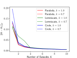
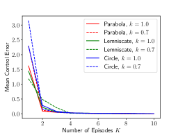
Figure 1: $\|\Theta-\Theta_{*}\|_{F}$ and Mean Control Error.

Here we vary the number of training episodes (the number of training masses) and observe its effect on the accuracy. It can be observed that our algorithm achieves an satisfactory accuracy using only $5$ episodes. We also illustrate trajectories obtained by our resulting controllers in Figure 2. From Figure 2, it is clear that as the agent plays more environments, it achieves better performance.

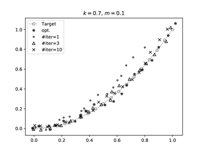
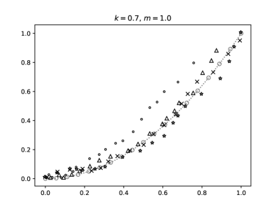
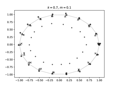
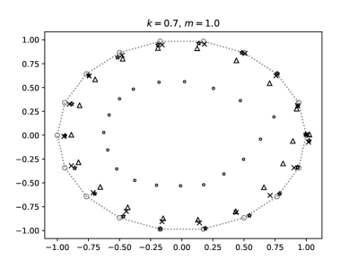
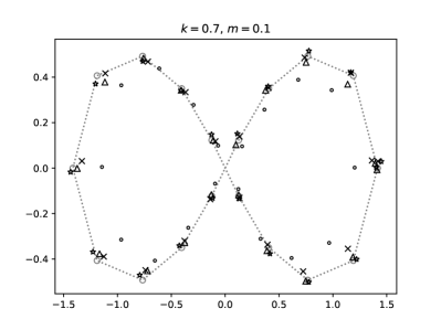
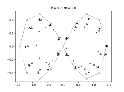
Figure 2: Example trajectories produced by the LQR controllers. We test the LQR policy to follow three types of paths: parabola, circle, and lemniscate. We first train a decoder, then test it on systems with $m=0.1,k=0.7$ (left column), and $m=1.0,k=0.7$ (right column). Dashed line with circles: target trajectories. $\star$: optimal policy. $\circ$: decoder trained on $1$ randomly drawn environment. $\triangle$: decoder trained on $3$ randomly drawn environments. $\times$: decoder trained on $10$ randomly drawn environments.

6 Conclusion

In this paper, we give a provably efficient algorithm for learning LQR with contexts. Our result bridges two major fields, learning with contexts and continuous control from a theoretically-principled view. For future work, it is interesting to study more complex settings, include non-linear control. Another interesting direction is to design provable algorithm in our setting with safety guarantees (Dann et al., 2018).

Appendix A Proof of Main Results

This sections devotes to proving the main results. Before we prove Proposition 4.1, let us use it to prove Theorem 4.1.

Proof of Theorem 4.1.

We rewrite the Equation equation 18 as follows.

$$\mathbb{E}_{C,D} \mathbb{E}_{\widetilde{\pi}}\Big{[}J^{\widetilde{\pi}}_{1}\big{(}M_{\Theta_{*},C,D},~{}x_{1}\big{)}\Big{]}-\mathbb{E}_{C,D}\Big{[}J^{*}_{1}\big{(}M_{\Theta_{*},C,D},~{}x_{1}\big{)}\Big{]}$$

$$=\frac{1}{K}\sum_{k=1}^{K}\mathbb{E}_{C,D}\Big{[}J_{1}^{\pi^{k}}\big{(}M_{\Theta_{*},C,D},~{}x_{1}\big{)}\Big{]}-\mathbb{E}_{C,D}\Big{[}J_{1}^{*}\big{(}M_{\Theta_{*},C,D},~{}x_{1}\big{)}\Big{]}$$

$$=\frac{1}{K}\sum_{k=1}^{K}\Big{(}\mathbb{E}_{C,D}\Big{[}J_{1}^{\pi^{k}}\big{(}M_{\Theta_{*},C,D},~{}x_{1}\big{)}\Big{]}-J_{1}^{\pi^{k}}\big{(}M_{\Theta_{*},C^{(k)},D^{(k)}},~{}x_{1}\big{)}+J_{1}^{\pi^{k}}\big{(}M_{\Theta_{*},C^{(k)},D^{(k)}},~{}x_{1}\big{)}$$

$$\qquad-J_{1}^{*}\big{(}M_{\Theta_{*},C^{(k)},D^{(k)}},~{}x_{1}\big{)}+J_{1}^{*}\big{(}M_{\Theta_{*},C^{(k)},D^{(k)}},~{}x_{1}\big{)}-\mathbb{E}_{C,D}\Big{[}J_{1}^{*}\big{(}M_{\Theta_{*},C,D},~{}x_{1}\big{)}\Big{]}\Big{)}$$

$$=R_{1}+R_{2}+R_{3}$$

where

$$R_{1}=\frac{1}{K}\sum_{k=1}^{K}\Big{(}\mathbb{E}_{C,D}\big{[}J_{1}^{\pi^{k}}\big{(}M_{\Theta_{*},C,D},~{}x_{1}\big{)}\Big{]}-J_{1}^{\pi^{k}}\big{(}M_{\Theta_{*},C^{(k)},D^{(k)}},~{}x_{1}\big{)}\Big{)},$$

$$R_{2}=\frac{1}{K}\sum_{k=1}^{K}\Big{(}J_{1}^{*}\big{(}M_{\Theta_{*},C^{(k)},D^{(k)}},~{}x_{1}\big{)}-\mathbb{E}_{C,D}\big{[}J_{1}^{*}\big{(}M_{\Theta_{*},C,D},~{}x_{1}\big{)}\Big{]}\Big{)},$$

and

$$R_{3}=\frac{1}{K}\sum_{k=1}^{K}\Big{(}J_{1}^{\pi^{k}}\big{(}M_{\Theta_{*},C^{(k)},D^{(k)}},~{}x_{1}\big{)}-J_{1}^{*}\big{(}M_{\Theta_{*},C^{(k)},D^{(k)}},~{}x_{1}\big{)}\Big{)}.$$

Let $\mathcal{F}_{k}$ be the filtration of fixing all randomness before episode $k$. We have $R_{1}$ and $R_{2}$ are Martingale difference sum. Note that the magnitude of each summand in $R_{1}$ or $R_{2}$ is upper bounded by (proved in Lemma A.3 and A.4),

$$Hc_{q}c_{x}$$

almost surely. Therefore, by Azuma’s inequality (Theorem A.1), we have, with probability greater than $1-\delta/2$,

$$|R_{1}|+|R_{2}|\leq 2Hc_{q}c_{x}\cdot\sqrt{\frac{2\log(8/\delta)}{K}}.$$

Moreover, by Proposition 4.1, we have with probability greater than $1-\delta/2$,

$$|R_{3}|\leq c\cdot d^{1/2}p\cdot\log^{3/2}(dKHc^{2}_{x}\delta^{-1})\cdot\sqrt{\frac{H}{K}},$$

where $c$ is constant depending only polynomially on $H$, $c_{q},c_{x},c_{M}$, and $c_{w}$. Combining the above two inequalities, and setting $K$ appropriately, we complete the proof of Theorem 4.1. ∎

A.1 Useful Concentration Bounds

Before we prove the main proposition, we first recall some useful concentration bounds.

Theorem A.1 (Azuma’s inequality).

Assume that $\{X_{s}\}_{s\geq 0}$ is a martingale and $|X_{s}-X_{s-1}|\leq c_{s}$ almost surely. Then for all $t>0$ and all $\epsilon>0$,

$$\Pr\big{[}|X_{t}-X_{0}|\geq\epsilon\big{]}\leq 2\exp\Bigg{(}\frac{-\epsilon^{2}}{2\sum_{s=1}^{t}c_{s}^{2}}\Bigg{)}.$$

Theorem A.2 (Martingale Concentration, Theorem 16 of Abbasi-Yadkori and Szepesvári [2011]).

Let ${\mathcal{F}_{t};t\geq 0}$ be a filtration, $(z_{t};t\geq 0)$ be an $\mathbb{R}^{d}$-valued stochastic process adapted to $(\mathcal{F}_{t})$. Let $(\eta_{t};t\geq 1)$ be a real-valued martingale difference process adapted to $\mathcal{F}_{t}$. Assume that $\eta_{t}$ is conditionally sub-Gaussian with constant $L$, i.e.,

$$\forall\gamma>0\quad:\mathbb{E}[\gamma\eta_{t}|\mathcal{F}_{t}]\leq\exp(\gamma^{2}L^{2}/2).$$

Consider the following martingale

$$S_{t}=\sum_{\tau=1}^{t}\eta_{\tau}z_{t-1}$$

and the matrix-valued processes

$$V_{t}=I+\sum_{\tau=0}^{t}z_{t-1}z_{t-1}^{\top}.$$

Then for any $\delta\in(0,1)$, with probability at least $1-\delta$,

$$\forall t\geq 0,\quad\|S_{t}\|^{2}_{V_{t}^{-1}}\leq 2L^{2}\log\bigg{(}\frac{\det(V_{t})^{1/2}}{\delta}\bigg{)}$$

where $\|S_{t}\|_{V_{t}^{-1}}^{2}:=S_{t}^{\top}V_{t}^{-1}S_{t}$.

A.2 Proof of Proposition 4.1

In this section, we prove the main proposition. We first bound $\det(V^{(k)})$ for any $k$.

Lemma A.1.

For all $k\in[K]$,

$$\det(V^{(k)})\leq\big{(}1+kHc^{2}_{x}/p\big{)}^{p}.$$

Proof.

Since $V^{(k)}$ is PD, we have,

$$\det(V^{(k)})\leq\Big{(}\mathrm{tr}(V^{(k)})/p\Big{)}^{p}\leq\bigg{(}1+\sum_{k^{\prime}=1}^{k}\sum_{h=1}^{H-1}\big{\|}z^{(k^{\prime})}_{h}\big{\|}_{2}^{2}/p\bigg{)}^{p}.$$

By Assumption 4.1, we have $\|z^{(k^{\prime})}_{h}\|_{2}^{2}\leq c^{2}_{x}$. This completes the proof. ∎

Let us then define an event $E_{k}$ as follows.

Definition A.1 (Good Event).

We define event $E_{k}$ as $\{\forall k^{\prime}\leq k:~{}\Theta_{*}\in\mathcal{C}^{(k^{\prime})}\}$.

We then show that the event $E_{k}$ happens with high probability.

Lemma A.2.

For all $k\in[K]$, we have $\Pr[E_{k}]\geq 1-\delta$.

Proof.

Now we consider $\Theta_{*}-\Theta^{(k)}$. We immediately have

$$\Theta_{*}^{\top}-\Theta^{(k)\top} =\Theta_{*}^{\top}-(V^{(k)})^{-1}\bigg{(}\sum_{k^{\prime}=1}^{k}\sum_{h=1}^{H-1}z^{(k^{\prime})}_{h}(\Theta_{*}z^{(k^{\prime})}_{h}+w_{h+1}^{(k^{\prime})})^{\top}\bigg{)}$$

$$=\bigg{(}I-(V^{(k)})^{-1}\sum_{k^{\prime}=1}^{k}\sum_{h=1}^{H-1}z^{(k^{\prime})}_{h}z^{(k^{\prime})\top}_{h}\bigg{)}\Theta_{*}^{\top}+(V^{(k)})^{-1}\sum_{k^{\prime}=1}^{k}\sum_{h=1}^{H-1}z^{(k^{\prime})}_{h}w_{h+1}^{(k^{\prime})\top}.$$

Next, we have

$$(\Theta_{*} -\Theta^{(k)})V^{(k)}(\Theta_{*}-\Theta^{(k)})^{\top}$$

$$= \Theta_{*}\bigg{(}I-(V^{(k)})^{-1}\sum_{k^{\prime}=1}^{k}\sum_{h=1}^{H-1}z^{(k^{\prime})}_{h}z^{(k^{\prime})\top}_{h}\bigg{)}^{\top}V^{(k)}\bigg{(}I-(V^{(k)})^{-1}\sum_{k^{\prime}=1}^{k}\sum_{h=1}^{H-1}z^{(k^{\prime})}_{h}z^{(k^{\prime})\top}_{h}\bigg{)}\Theta_{*}^{\top}$$

$$+\Theta_{*}\bigg{(}I-(V^{(k)})^{-1}\sum_{k^{\prime}=1}^{k}\sum_{h=1}^{H-1}z^{(k^{\prime})}_{h}z^{(k^{\prime})\top}_{h}\bigg{)}^{\top}\sum_{k^{\prime}=1}^{k}\sum_{h=1}^{H-1}z^{(k^{\prime})}_{h}w_{h+1}^{(k^{\prime})\top}$$

$$+\sum_{k^{\prime}=1}^{k}\sum_{h=1}^{H-1}w_{h+1}^{(k^{\prime})}z^{(k^{\prime})\top}_{h}\bigg{(}I-(V^{(k)})^{-1}\sum_{k^{\prime}=1}^{k}\sum_{h=1}^{H-1}z^{(k^{\prime})}_{h}z^{(k^{\prime})\top}_{h}\bigg{)}\Theta_{*}^{\top}$$

$$+\sum_{k^{\prime}=1}^{k}\sum_{h=1}^{H-1}w_{h+1}^{(k^{\prime})}z^{(k^{\prime})\top}_{h}(V^{(k)})^{-1}\sum_{k^{\prime}=1}^{k}\sum_{h=1}^{H-1}z^{(k^{\prime})}_{h}w_{h+1}^{(k^{\prime})\top}$$

Note that $\sum_{k^{\prime}=1}^{k}\sum_{h=1}^{H-1}z^{(k^{\prime})}_{h}z^{(k^{\prime})\top}_{h}=V^{(k)}-I$ and thus $(V^{(k)})^{-1}\sum_{k^{\prime}=1}^{k}\sum_{h=1}^{H-1}z^{(k^{\prime})}_{h}z^{(k^{\prime})\top}_{h}=I-(V^{(k)})^{-1}$. Hence we have

$$\mathrm{tr}\big{[}( \Theta_{*}-\Theta^{(k)})V^{(k)}(\Theta_{*}-\Theta^{(k)})^{\top}\big{]}$$

$$=\|\Theta^{*}\|_{(V^{(k)})^{-1}}^{2}+2\mathrm{tr}\Big{(}\Theta_{*}(V^{(k)})^{-1}\sum_{k^{\prime}=1}^{k}\sum_{h=1}^{H-1}z^{(k^{\prime})}_{h}w_{h+1}^{(k^{\prime})\top}\Big{)}+\Big{\|}\sum_{k^{\prime}=1}^{k}\sum_{h=1}^{H-1}z^{(k^{\prime})}_{h}w_{h+1}^{(k^{\prime})\top}\Big{\|}_{(V^{(k)})^{-1}}^{2}$$

$$\leq\|\Theta_{*}\|_{(V^{(k)})^{-1}}^{2}+2\Big{\|}\Theta_{*}\Big{\|}_{(V^{(k)})^{-1}}\Big{\|}\sum_{k^{\prime}=1}^{k}\sum_{h=1}^{H-1}z^{(k^{\prime})}_{h}w_{h+1}^{(k^{\prime})\top}\Big{\|}_{(V^{(k)})^{-1}}+\Big{\|}\sum_{k^{\prime}=1}^{k}\sum_{h=1}^{H-1}z^{(k^{\prime})}_{h}w_{h+1}^{(k^{\prime})\top}\Big{\|}_{(V^{(k)})^{-1}}^{2}$$

where $\|X\|_{V}^{2}:=\mathrm{tr}\big{(}X^{\top}VX\big{)}$ and the last inequality uses Cauchy-Schwartz inequality. Notice that

$$\|\Theta_{*}\|_{(V^{(k)})^{-1}}\leq\|\Theta_{*}\|_{F}.$$

Moreover, we have

$$\Big{\|}\sum_{k^{\prime}=1}^{k}\sum_{h=1}^{H-1}z^{(k^{\prime})}_{h}w_{h+1}^{(k^{\prime})\top}\Big{\|}_{(V^{(k)})^{-1}}^{2} =\bigg{\|}(V^{(k)})^{-1/2}\sum_{k^{\prime}=1}^{k}\sum_{h=1}^{H-1}z^{(k^{\prime})}_{h}w_{h+1}^{(k^{\prime})\top}\bigg{\|}_{F}^{2}$$

$$=\sum_{j\in[d]}\bigg{\|}(V^{(k)})^{-1/2}\sum_{k^{\prime}=1}^{k}\sum_{h=1}^{H-1}w_{h+1,j}^{(k^{\prime})}z^{(k^{\prime})}_{h}\bigg{\|}_{2}^{2}$$

$$=\sum_{j\in[d]}\Big{\|}\sum_{k^{\prime}=1}^{k}\sum_{h=1}^{H-1}w_{h+1,j}^{(k^{\prime})}z^{(k^{\prime})}_{h}\Big{\|}_{(V^{(k)})^{-1}}^{2}$$

By Theorem A.2, we have, for every $j\in[d]$, with probability at least $1-\delta/d$, we have,

$$\Big{\|}\sum_{k^{\prime}=1}^{k}\sum_{h=1}^{H-1}w_{h+1,j}^{(k^{\prime})}z^{(k^{\prime})}_{h}\Big{\|}_{(V^{(k)})^{-1}}^{2}\leq 2c_{w}^{2}\log(d\det(V^{(k)})^{1/2}/\delta).$$

By an union bound, we have, with probability at least $1-\delta$,

$$\Big{\|}\sum_{k^{\prime}=1}^{k}\sum_{h=1}^{H-1}w_{h+1}^{(k^{\prime})}z^{(k^{\prime})}_{h}\Big{\|}_{(V^{(k)})^{-1}}^{2}\leq 2dc_{w}^{2}\log(d\det(V^{(k)})^{1/2}/\delta).$$

Plugging to $\mathrm{tr}\big{[}(\Theta_{*}-\Theta^{(k)})V^{(k)}(\Theta_{*}-\Theta^{(k)})^{\top}\big{]}$, we have, with probability at least $1-\delta$,

$$\mathrm{tr}\big{[}(\Theta_{*}-\Theta^{(k)})V^{(k)}(\Theta_{*}-\Theta^{(k)})^{\top}\big{]} \leq\Big{(}c_{\Theta}+c_{w}\sqrt{2d\log(d\det(V^{(k)})^{1/2}/\delta)}\Big{)}^{2}$$

$$\leq\Big{(}c_{\Theta}+c_{w}\sqrt{2d\big{(}\log d+p\log(1+kHc^{2}_{x}/p)/2+\log\delta^{-1}\big{)}}\Big{)}^{2}.$$

This completes the proof. ∎

We define $\mathbb{I}_{E_{K}}$ as the indicator for $E_{K}$ happens. We denote

$$M_{*}^{(k)}=M_{\Theta_{*},C^{(k)},D^{(k)}},\quad M^{(k)}=M_{\Theta^{(k)},C^{(k)},D^{(k)}},\quad\text{and}\quad y^{(k)}_{h}=[x_{h}^{(k)\top},u_{h}^{(k)\top}]^{\top}.$$

On $E_{k}$, we have

$$\forall k\in[K]:\quad J_{1}^{*}(\widetilde{M}^{(k)},x_{1}^{k})\leq J_{1}^{*}({M}_{*}^{(k)},x_{1}^{k}).$$

We denote $\Delta^{(k)}:=J_{h}^{\pi^{k}}(M_{*}^{(k)},x_{1})-J_{h}^{*}(M_{*}^{(k)},x_{1})$. We can rewrite $equation~{}\ref{eq:reg}$ as

$$\mathrm{Regret}(KH)=\sum_{k=1}^{K}\mathbb{I}_{E_{k}}\Delta^{(k)}+\sum_{k=1}^{K}(1-\mathbb{I}_{E_{k}})\Delta^{(k)},$$

where the second term is non-zero with probability less than $\delta$. For the first term, we have

$$\mathbb{I}_{E_{k}}\Delta^{(k)}\leq\mathbb{I}_{E_{k}}\big{[}J_{1}^{\pi^{k}}(M_{*}^{(k)},x_{1})-J_{1}^{*}(\widetilde{M}^{(k)},x_{1}))\big{]}=:\mathbb{I}_{E_{k}}\cdot\widetilde{\Delta}^{(k)}_{1},$$

where

$$\widetilde{\Delta}^{(k)}_{h}=J_{h}^{\pi^{k}}(M_{*}^{(k)},x_{h})-J^{*}_{h}(\widetilde{M}^{(k)},x_{h}).$$

Let us consider $\widetilde{\Delta}_{h}^{(k)}$. We denote filtration $\mathcal{F}_{k,h}$ as fixing the trajectory up to time $(k,h)$ and all $\{C^{(k^{\prime})},D^{(k^{\prime})}\}_{k^{\prime}\leq k}$.

We have

$$\widetilde{\Delta}_{h}^{(k)}= x^{(k)\top}_{h}Q_{h}x_{h}^{(k)}+u^{(k)\top}_{h}R_{h}u_{h}^{(k)}+\mathbb{E}_{w_{h+1}^{(k)}}[J_{h+1}^{\pi^{k}}(M_{*}^{(k)},x_{h+1}^{(k)})~{}|~{}\mathcal{F}_{k,h}]$$

$$-x^{(k)\top}_{h}Q_{h}x_{h}^{(k)}-u^{(k)\top}_{h}R_{h}u_{h}^{(k)}$$

$$-\mathbb{E}_{w_{h+1}^{(k)}}\Big{[}(\widetilde{M}^{(k)}z^{(k)}_{h}+w^{(k)}_{h+1})^{\top}P_{h+1}(\widetilde{M}^{(k)})(\widetilde{M}^{(k)}z^{(k)}_{h}+w^{(k)}_{h+1})~{}|~{}\mathcal{F}_{k,h}\Big{]}$$

$$-C_{h+1}(\widetilde{M}^{(k)})$$

$$= \mathbb{E}_{w_{h+1}^{(k)}}[J_{h+1}^{\pi^{k}}(M_{*}^{(k)},x_{h+1}^{(k)})~{}|~{}\mathcal{F}_{k,h}]$$

$$-\mathbb{E}_{w_{h+1}^{(k)}}\Big{[}(\widetilde{M}^{(k)}z^{(k)}_{h}+w^{(k)}_{h+1})^{\top}P_{h+1}(\widetilde{M}^{(k)})(\widetilde{M}^{(k)}z^{(k)}_{h}+w^{(k)}_{h+1})~{}|~{}\mathcal{F}_{k,h}\Big{]}$$

$$-C_{h+1}(\widetilde{M}^{(k)})$$

$$= \mathbb{E}_{w_{h+1}^{(k)}}[J_{h+1}^{\pi^{k}}(M_{*}^{(k)},x_{h+1}^{(k)})~{}|~{}\mathcal{F}_{k,h}]-J_{h+1}^{\pi^{k}}(M_{*}^{(k)},x_{h+1}^{(k)})+J_{h+1}^{\pi^{k}}(M_{*}^{(k)},x_{h+1}^{(k)})$$

$$-\big{(}\widetilde{M}^{(k)}z^{(k)}_{h}\big{)}^{\top}P_{h+1}(\widetilde{M}^{(k)})\big{(}\widetilde{M}^{(k)}z^{(k)}_{h}\big{)}-C_{h+1}(\widetilde{M}^{(k)})$$

$$-\mathbb{E}_{w_{h+1}^{(k)}}\Big{[}\big{(}w^{(k)}_{h+1}\big{)}^{\top}P_{h+1}(\widetilde{M}^{(k)})w^{(k)}_{h+1}~{}\big{|}~{}\mathcal{F}_{k,h}\Big{]}$$

$$= \delta_{h}^{(k)}+J_{h+1}^{\pi^{k}}(M_{*}^{(k)},x_{h+1}^{(k)})-\big{(}\widetilde{M}^{(k)}z^{(k)}_{h}\big{)}^{\top}P_{h+1}(\widetilde{M}^{(k)})\big{(}\widetilde{M}^{(k)}z^{(k)}_{h}\big{)}-C_{h+1}(\widetilde{M}^{(k)})$$

$$-\mathbb{E}_{w_{h+1}^{(k)}}\Big{[}\big{(}x_{h+1}^{(k)}-M_{*}^{(k)}z^{(k)}_{h}\big{)}^{\top}P_{h+1}(\widetilde{M}^{(k)})\big{(}x_{h+1}^{(k)}-M_{*}^{(k)}z^{(k)}_{h}\big{)}~{}\big{|}~{}\mathcal{F}_{k,h}\Big{]}$$

$$= \delta_{h}^{(k)}+J_{h+1}^{\pi^{k}}(M_{*}^{(k)},x_{h+1}^{(k)})-\big{(}\widetilde{M}^{(k)}z^{(k)}_{h}\big{)}^{\top}P_{h+1}(\widetilde{M}^{(k)})\big{(}\widetilde{M}^{(k)}z^{(k)}_{h}\big{)}-C_{h+1}(\widetilde{M}^{(k)})$$

$$-\mathbb{E}_{w_{h+1}^{(k)}}\Big{[}\big{(}x_{h+1}^{(k)}\big{)}^{\top}P_{h+1}(\widetilde{M}^{(k)})\big{(}x_{h+1}^{(k)}\big{)}~{}\big{|}~{}\mathcal{F}_{k,h}\Big{]}+\big{(}M_{*}^{(k)}z^{(k)}_{h}\big{)}^{\top}P_{h+1}(\widetilde{M}^{(k)})\big{(}M_{*}^{(k)}z^{(k)}_{h}\big{)}$$

$$= \delta_{h}^{(k)}+\delta_{h}^{{}^{\prime}(k)}+\delta_{h}^{{}^{\prime\prime}(k)}+J_{h+1}^{\pi^{k}}(M_{*},x_{h+1}^{(k)})-J_{h+1}^{*}(\widetilde{M}^{(k)},x_{h+1}^{(k)})~{}~{}~{}~{}~{}~{}~{}~{}~{}~{}~{}~{}~{}~{}~{}~{}~{}~{}~{}~{}~{}~{}~{}~{}~{}~{}$$

where

$$\delta_{h}^{(k)} =\mathbb{E}_{w_{h+1}^{(k)}}[J_{h+1}^{\pi^{k}}(M_{*}^{(k)},x_{h+1}^{(k)})~{}|~{}\mathcal{F}_{k,h}]-J_{h+1}^{\pi^{k}}(M_{*}^{(k)},x_{h+1}^{(k)})$$ (20)

$$\delta_{h}^{{}^{\prime}(k)} =\big{(}x_{h+1}^{(k)}\big{)}^{\top}P_{h+1}(\widetilde{M}^{(k)})\big{(}x_{h+1}^{(k)}\big{)}-\mathbb{E}_{w_{h+1}^{(k)}}\Big{[}\big{(}x_{h+1}^{(k)}\big{)}^{\top}P_{h+1}(\widetilde{M}^{(k)})\big{(}x_{h+1}^{(k)}\big{)}~{}\big{|}~{}\mathcal{F}_{k,h}\Big{]}$$ (21)

$$\delta_{h}^{{}^{\prime\prime}(k)} =\big{(}M_{*}^{(k)}z^{(k)}_{h}\big{)}^{\top}P_{h+1}(\widetilde{M}^{(k)})\big{(}M_{*}^{(k)}z^{(k)}_{h}\big{)}-\big{(}\widetilde{M}^{(k)}z^{(k)}_{h}\big{)}^{\top}P_{h+1}(\widetilde{M}^{(k)})\big{(}\widetilde{M}^{(k)}z^{(k)}_{h}\big{)}.$$ (22)

By induction, we have

$$\sum_{k^{\prime}=1}^{k}\widetilde{\Delta}_{1}^{(k)}\leq\sum_{k^{\prime}=1}^{k}\sum_{h=1}^{H-1}\big{(}\delta_{h}^{(k)}+\delta_{h}^{{}^{\prime}(k)}+\delta_{h}^{{}^{\prime\prime}(k)}\big{)}.$$

Notice that $\delta^{(k)}_{h}$ and $\delta_{h}^{(k)}$ are Martingale difference adapted to $\mathcal{F}_{k,h}$. We can well bound the sum of them via Azuma’s inequality.

Lemma A.3.

For all $h\in[H]$, $|J_{h}^{\pi^{k}}(M_{*}^{(k)},x_{h}^{(k)})|\leq(H-h+1)\cdot c_{q}\cdot c_{x}.$

Proof.

Prove by induction on $h$. The base case $J_{H}^{\pi^{k}}(M_{*}^{(k)},x_{H}^{(k)})=x_{H}^{(k)\top}Q_{H}x_{H}^{(k)}\leq c_{q}c_{x}^{2}$ holds straightforwardly. Consider an arbitrary $h<H$, we have

$$J_{h}^{\pi^{k}}(M_{*}^{(k)},x_{h}^{(k)})=x^{(k)\top}_{h}Q_{h}x_{h}^{(k)}+u^{(k)\top}_{h}R_{h}u_{h}^{(k)}+\mathbb{E}_{w_{h+1}^{(k)}}[J_{h+1}^{\pi^{k}}(M_{*}^{(k)},x_{h+1}^{(k)})~{}|~{}\mathcal{F}_{k,h}]\leq c_{q}c_{x}+(H-h)\cdot c_{q}\cdot c_{x}$$

as desired. ∎

Lemma A.4.

For all $x\in X$, we have $\mathbb{I}_{E_{K}}|J_{h}^{*}(\widetilde{M}^{(k)},x)|\leq c_{q}c_{x}$.

Proof.

Follows from Assumption 4.1. ∎

We are now ready to prove Proposition 4.1.

Proof of Proposition 4.1.

Thus by Azuma’s inequality, we have, with probability at least $1-\delta$,

$$\Big{|}\sum_{k^{\prime}=1}^{k}\sum_{h=1}^{H-1}\delta^{(k)}_{h}\Big{|}\leq\sqrt{2kH\cdot\big{[}(H-h+1)qc_{x}+c_{q}c_{x}\big{]}^{2}\cdot\log\frac{2}{\delta}}.$$

And, with probability at least $1-\delta$,

$$\Big{|}\sum_{k^{\prime}=1}^{k}\sum_{h=1}^{H-1}\delta^{{}^{\prime}(k)}_{h}\Big{|}\leq\sqrt{8kH\cdot c_{x}^{2}c_{q}^{2}\cdot\log\frac{2}{\delta}}.$$

For $\sum\delta^{{}^{\prime\prime}(k)}_{h}$, we bound it here.

$$\Big{|}\sum_{k^{\prime}=1}^{k}\sum_{h=1}^{H-1}\delta^{{}^{\prime\prime}(k)}_{h}\Big{|}\leq \sum_{k^{\prime}=1}^{k}\sum_{h=1}^{H-1}\Big{|}\delta^{{}^{\prime\prime}(k)}_{h}\Big{|}=\sum_{k^{\prime}=1}^{k}\sum_{h=1}^{H-1}\Big{|}\|P_{h+1}(\widetilde{M}^{(k)})^{1/2}\big{(}\widetilde{M}^{(k)}y^{(k)}_{h}\big{)}\|_{2}^{2}-\|P_{h+1}(\widetilde{M}^{(k)})^{1/2}\big{(}{M}^{*}y^{(k)}_{h}\big{)}\|_{2}^{2}\Big{|}$$

$$\leq \sum_{k^{\prime}=1}^{k}\sum_{h=1}^{H-1}\Big{|}\big{(}\|P_{h+1}(\widetilde{M}^{(k)})^{1/2}\big{(}\widetilde{M}^{(k)}y^{(k)}_{h}\big{)}\|_{2}-\|P_{h+1}(\widetilde{M}^{(k)})^{1/2}\big{(}{M}^{*}y^{(k)}_{h}\big{)}\|_{2}\big{)}$$

$$\cdot \big{(}\|P_{h+1}(\widetilde{M}^{(k)})^{1/2}\big{(}\widetilde{M}^{(k)}y^{(k)}_{h}\big{)}\|_{2}+\|P_{h+1}(\widetilde{M}^{(k)})^{1/2}\big{(}{M}^{*}y^{(k)}_{h}\big{)}\|_{2}\big{)}\Big{|}$$

$$\leq \Big{[}\sum_{k^{\prime}=1}^{k}\sum_{h=1}^{H-1}\Big{(}\|P_{h+1}(\widetilde{M}^{(k)})^{1/2}\big{(}\widetilde{M}^{(k)}y^{(k)}_{h}\big{)}\|_{2}-\|P_{h+1}(\widetilde{M}^{(k)})^{1/2}\big{(}{M}^{*}y^{(k)}_{h}\big{)}\|_{2}\Big{)}^{2}\Big{]}^{1/2}$$

$$\cdot \Big{[}\sum_{k^{\prime}=1}^{k}\sum_{h=1}^{H-1}\Big{(}\|P_{h+1}(\widetilde{M}^{(k)})^{1/2}\big{(}\widetilde{M}^{(k)}y^{(k)}_{h}\big{)}\|_{2}+\|P_{h+1}(\widetilde{M}^{(k)})^{1/2}\big{(}{M}^{*}y^{(k)}_{h}\big{)}\|_{2}\Big{)}^{2}\Big{]}^{1/2}$$

Notice that $\|P_{h+1}(\widetilde{M}^{(k)})^{1/2}\big{(}\widetilde{M}^{(k)}y^{(k)}_{h}\big{)}\|_{2}\leq c_{q}c_{x}c_{\Theta}$ and $\|P_{h+1}(\widetilde{M}^{(k)})^{1/2}\big{(}{M}^{*}y^{(k)}_{h}\big{)}\|_{2}\leq c_{q}c_{x}$. Hence

$$\Big{[}\sum_{k^{\prime}=1}^{k}\sum_{h=1}^{H-1} \Big{|}\Big{(}\|P_{h+1}(\widetilde{M}^{(k)})^{1/2}\big{(}\widetilde{M}^{(k)}y^{(k)}_{h}\big{)}\|_{2}+\|P_{h+1}(\widetilde{M}^{(k)})^{1/2}\big{(}{M}^{*}y^{(k)}_{h}\big{)}\|_{2}\Big{)}^{2}\Big{]}^{1/2}$$

$$\leq\sqrt{kH\cdot(c_{q}c_{x}(1+c_{\Theta}))^{2}}.$$

Moreover, by triangle inequality, we have

$$\Big{|} \|P_{h+1}(\widetilde{M}^{(k)})^{1/2}\big{(}\widetilde{M}^{(k)}y^{(k)}_{h}\big{)}\|_{2}-\|P_{h+1}(\widetilde{M}^{(k)})^{1/2}\big{(}{M}^{*}y^{(k)}_{h}\big{)}\|_{2}\Big{|}$$

$$\leq\|P_{h+1}(\widetilde{M}^{(k)})^{1/2}\big{(}\widetilde{M}^{(k)}-{M}^{*}\big{)}y^{(k)}_{h}\|_{2}$$

$$\leq c_{q}\|\big{(}\widetilde{M}^{(k)}-{M}^{*}\big{)}y^{(k)}_{h}\|_{2}$$

$$\leq c_{q}\|\big{(}\widetilde{M}^{(k)}-{M}^{*}\big{)}(V^{(k)})^{1/2}(V^{(k)})^{-1/2}y_{h}^{(k)}\|_{2}$$

$$\leq c_{q}\|\big{(}\widetilde{M}^{(k)}-{M}^{*}\big{)}(V^{(k)})^{1/2}\|_{2}\|(V^{(k)})^{-1/2}y_{h}^{(k)}\|_{2}$$

$$\leq c_{q}\cdot\sqrt{\beta^{(k)}}\cdot\|(V^{(k)})^{-1/2}y_{h}^{(k)}\|_{2}.$$

By Assumption 2, we also have $\|(V^{(k)})^{-1/2}y_{h}^{(k)}\|_{2}\leq\|(y_{h}^{(k)}\|_{2}\leq\sqrt{c_{x}}$. Hence,

$$\Big{|}\|P_{h+1}(\widetilde{M}^{(k)})^{1/2} \big{(}\widetilde{M}^{(k)}y^{(k)}_{h}\big{)}\|_{2}-\|P_{h+1}(\widetilde{M}^{(k)})^{1/2}\big{(}{M}^{*}y^{(k)}_{h}\big{)}\|_{2}\Big{|}$$

$$\leq c_{q}\sqrt{c_{x}}\cdot\sqrt{\beta^{(k)}}\cdot\min\big{(}\|(V^{(k)})^{-1/2}y_{h}^{(k)}\|_{2},1\big{)}$$

Combining the above equations, we have,

$$\Big{|}\sum_{k^{\prime}=1}^{k}\sum_{h=1}^{H-1}\delta^{{}^{\prime\prime}(k)}_{h}\Big{|} \leq\sqrt{kH\cdot(c_{q}c_{x}(1+c_{\Theta}))^{2}}\cdot c_{q}\sqrt{c_{x}}\cdot\sqrt{\beta^{(k)}}\cdot\sqrt{\sum_{k^{\prime}=1}^{k}\sum_{h=1}^{H-1}\min\big{(}\|(V^{(k)})^{-1/2}y_{h}^{(k)}\|_{2}^{2},1\big{)}}$$

$$\leq 2c_{x}^{3/2}c_{q}^{2}c_{\Theta}\cdot\sqrt{\beta^{(k)}}\cdot\sqrt{\sum_{k^{\prime}=1}^{k}\sum_{h=1}^{H-1}\log\Big{(}1+\|(V^{(k)})^{-1/2}y_{h}^{(k)}\|_{2}^{2}\Big{)}}\cdot\sqrt{kH}.$$

Lastly, by Lemma 8 of Yang and Wang [2019], we have

$$\sum_{k^{\prime}=1}^{k}\sum_{h=1}^{H-1}\log\Big{(}1+\|(V^{(k)})^{-1/2}y_{h}^{(k)}\|_{2}^{2}\Big{)}\leq 2H\log\mathrm{det}(V^{(k)}).$$

Together with Lemma A.1, we have

$$2H\log\det(V^{(k)})\leq 2Hp\cdot\log\big{(}1+kHc_{x}^{2}/p\big{)}.$$

Overall, we have,

$$\Big{|}\sum_{k^{\prime}=1}^{k}\sum_{h=1}^{H-1}\delta^{{}^{\prime\prime}(k)}_{h}\Big{|} \leq 2c_{x}^{3/2}c_{q}^{2}c_{\Theta}\cdot\sqrt{2Hp\cdot\log\big{(}1+kHc^{2}_{x}/p\big{)}\cdot(\beta^{(k)})\cdot kH}.$$

Putting everything together, with probability at least $1-2\delta$, we have

$$\mathrm{reg}(KH) \leq\sum_{k^{\prime}=1}^{K}\sum_{h=1}^{H-1}\big{(}\delta_{h}^{(k)}+\delta_{h}^{{}^{\prime}(k)}+\delta_{h}^{{}^{\prime\prime}(k)}\big{)}$$

$$\leq\sqrt{2KH\cdot\big{[}(H-h+1)c_{q}c_{x}+c_{q}c_{x}\big{]}^{2}\cdot\log\frac{2}{\delta}}+\sqrt{8KH\cdot c_{x}^{2}c_{q}^{2}\cdot\log\frac{2}{\delta}}$$

$$\quad+2c_{x}^{3/2}c_{q}^{2}c_{\Theta}\cdot\sqrt{2Hp\cdot\log\big{(}1+KHc^{2}_{x}/p\big{)}\cdot(\beta^{(K)})\cdot KH}$$

$$\leq c_{H}\cdot d^{1/2}p\cdot\log^{3/2}(dKHc^{2}_{x}\delta^{-1})\cdot\sqrt{KH},$$

where $c_{H}$ is a constant depending on $H,c_{q},c_{x},c_{\Theta}$ and $c_{w}$. ∎

Appendix B Concrete Choice of the Parameters

We further augment the state so that the first coordinate is a constant with value $1$. More specifically, we set the state $x_{h}=[1;z_{h};v_{h}]\in\mathbb{R}^{5}$. We set

$$Q_{h}=\left(\begin{array}[]{c c c}\|z_{h}^{*}\|_{2}^{2}&-z_{h}^{*}&0\\ -z_{h}^{*}&I&0\\ 0&0&0\\ \end{array}\right)$$

so that for any state $x_{h}$, $x_{h}^{T}Q_{h}x_{H}=\|z_{h}-z_{h}^{*}\|_{2}^{2}$. We set $R_{h}=I_{2}$ We set

$$\Theta_{*}=\left(\begin{array}[]{c c c c c c c}1&0&0&0&0&0&0\\ 0&1&0&1&0&0&0\\ 0&0&1&0&1&0&0\\ 0&0&0&k&0&1&0\\ 0&0&0&0&k&0&1\\ \end{array}\right),$$

$C$ to be the $5\times 5$ identity matrix and $D$ to be $I/m$ with size $2\times 2$ where $m$ is sampled from the uniform distribution over $[0.1,10]$, to represent the physical law in Equation 19.

References

- Abbasi-Yadkori and Neu (2014) Yasin Abbasi-Yadkori and Gergely Neu. Online learning in mdps with side information. arXiv preprint arXiv:1406.6812, 2014.
- Abbasi-Yadkori and Szepesvári (2011) Yasin Abbasi-Yadkori and Csaba Szepesvári. Regret Bounds for the Adaptive Control of Linear Quadratic Systems. Technical report, 2011. URL http://proceedings.mlr.press/v19/abbasi-yadkori11a/abbasi-yadkori11a.pdf.
- Abbasi-Yadkori et al. (2018) Yasin Abbasi-Yadkori, Nevena Lazic, and Csaba Szepesvári. Regret bounds for model-free linear quadratic control. arXiv preprint arXiv:1804.06021, 2018.
- Abel et al. (2018) David Abel, Dilip Arumugam, Lucas Lehnert, and Michael Littman. State abstractions for lifelong reinforcement learning. In Jennifer Dy and Andreas Krause, editors, Proceedings of the 35th International Conference on Machine Learning, volume 80 of Proceedings of Machine Learning Research, pages 10–19, Stockholmsmässan, Stockholm Sweden, 10–15 Jul 2018. PMLR. URL http://proceedings.mlr.press/v80/abel18a.html.
- Bertsekas (1996) Dimitri P Bertsekas. Dynamic programming and optimal control. Journal of the Operational Research Society, 47(6):833–833, 1996.
- Cohen et al. (2019) Alon Cohen, Tomer Koren, and Yishay Mansour. Learning linear-quadratic regulators efficiently with only regret. arXiv preprint arXiv:1902.06223, 2019.
- Dann et al. (2018) Christoph Dann, Lihong Li, Wei Wei, and Emma Brunskill. Policy certificates: Towards accountable reinforcement learning. arXiv preprint arXiv:1811.03056, 2018.
- Dean et al. (2017) Sarah Dean, Horia Mania, Nikolai Matni, Benjamin Recht, and Stephen Tu. On the sample complexity of the linear quadratic regulator. arXiv preprint arXiv:1710.01688, 2017.
- Dean et al. (2018) Sarah Dean, Horia Mania, Nikolai Matni, Benjamin Recht, and Stephen Tu. Regret bounds for robust adaptive control of the linear quadratic regulator. In S. Bengio, H. Wallach, H. Larochelle, K. Grauman, N. Cesa-Bianchi, and R. Garnett, editors, Advances in Neural Information Processing Systems 31, pages 4188–4197. Curran Associates, Inc., 2018. URL http://papers.nips.cc/paper/7673-regret-bounds-for-robust-adaptive-control-of-the-linear-quadratic-regulator.pdf.
- Fiechter (1997) Claude-Nicolas Fiechter. Pac adaptive control of linear systems. In Annual Workshop on Computational Learning Theory: Proceedings of the tenth annual conference on Computational learning theory, volume 6, pages 72–80. Citeseer, 1997.
- Gamrian and Goldberg (2018) Shani Gamrian and Yoav Goldberg. Transfer learning for related reinforcement learning tasks via image-to-image translation. arXiv preprint arXiv:1806.07377, 2018.
- Hallak et al. (2015) Assaf Hallak, Dotan Di Castro, and Shie Mannor. Contextual markov decision processes. arXiv preprint arXiv:1502.02259, 2015.
- Killian et al. (2016) Taylor Killian, George Konidaris, and Finale Doshi-Velez. Transfer learning across patient variations with hidden parameter markov decision processes. arXiv preprint arXiv:1612.00475, 2016.
- Lehnert and Littman (2018) Lucas Lehnert and Michael L Littman. Transfer with model features in reinforcement learning. arXiv preprint arXiv:1807.01736, 2018.
- Lehnert et al. (2019) Lucas Lehnert, Michael J Frank, and Michael L Littman. Reward predictive representations generalize across tasks in reinforcement learning. BioRxiv, page 653493, 2019.
- Modi and Tewari (2019) Aditya Modi and Ambuj Tewari. Contextual markov decision processes using generalized linear models. arXiv preprint arXiv:1903.06187, 2019.
- Modi et al. (2018) Aditya Modi, Nan Jiang, Satinder Singh, and Ambuj Tewari. Markov decision processes with continuous side information. In Algorithmic Learning Theory, pages 597–618, 2018.
- Puterman (2014) Martin L Puterman. Markov Decision Processes.: Discrete Stochastic Dynamic Programming. John Wiley & Sons, 2014.
- Santara et al. (2019) Anirban Santara, Rishabh Madan, Balaraman Ravindran, and Pabitra Mitra. Extra: Transfer-guided exploration. arXiv preprint arXiv:1906.11785, 2019.
- Spector and Belongie (2018) Benjamin Spector and Serge Belongie. Sample-efficient reinforcement learning through transfer and architectural priors. arXiv preprint arXiv:1801.02268, 2018.
- Taylor and Stone (2009) Matthew E Taylor and Peter Stone. Transfer learning for reinforcement learning domains: A survey. Journal of Machine Learning Research, 10(Jul):1633–1685, 2009.
- Tu and Recht (2017) Stephen Tu and Benjamin Recht. Least-squares temporal difference learning for the linear quadratic regulator. arXiv preprint arXiv:1712.08642, 2017.
- Tu and Recht (2018) Stephen Tu and Benjamin Recht. The gap between model-based and model-free methods on the linear quadratic regulator: An asymptotic viewpoint. arXiv preprint arXiv:1812.03565, 2018.
- Wu et al. (2018) Yi Wu, Yuxin Wu, Aviv Tamar, Stuart Russell, Georgia Gkioxari, and Yuandong Tian. Learning and planning with a semantic model. arXiv preprint arXiv:1809.10842, 2018.
- Yang and Wang (2019) Lin F Yang and Mengdi Wang. Reinforcement leaning in feature space: Matrix bandit, kernels, and regret bound. arXiv preprint arXiv:1905.10389, 2019.
- Yu et al. (2018) Yang Yu, Shi-Yong Chen, Qing Da, and Zhi-Hua Zhou. Reusable reinforcement learning via shallow trails. IEEE transactions on neural networks and learning systems, 29(6):2204–2215, 2018.