Pathological subgradient dynamics

Abstract. We construct examples of Lipschitz continuous functions, with pathological subgradient dynamics both in continuous and discrete time. In both settings, the iterates generate bounded trajectories, and yet fail to detect any (generalized) critical points of the function.

Key words. subgradient algorithm, Lipschitz function, Clarke subdifferential, splitting set.

AMS Subject Classification.   90C30, 49J52, 65K10;

1 Introduction

The subgradient method plays a central role in large-scale optimization and its numerous applications. The primary goal of the method for nonsmooth and nonconvex optimization is to find generalized critical points. For example, for a locally Lipschitz continuous function $f$, we may be interested in finding a point $x$ satisfying the inclusion $0\in\partial f(x)$, where the symbol $\partial f(x)$ denotes the Clarke subdifferential. The main difficulty in analyzing subgradient-type methods is that it is unclear how to construct a Lyapunov potential for the iterates when the target function is merely Lipschitz continuous. One popular strategy to circumvent this difficulty is to pass to continuous time where a Lyapunov function may be more apparent. Indeed, for reasonable function classes, the objective itself decreases along the continuous time subgradient trajectories of the function. For example, this is the path classically followed by Benaïm et al. [3, 4], Borkar [8], Ljung [27], and more recently by Davis et al. [17] and Duchi-Ruan [18].

Setting the formalism, consider the task of minimizing a Lipschitz continuous function $f$ on ${\mathbb{R}}^{d}$ by the subgradient method. It is intuitively clear that the asymptotic performance of the algorithm is dictated by the long term behavior of the absolutely continuous trajectories $\gamma\colon[0,\infty)\to{\mathbb{R}}^{d}$ of the associated subgradient dynamical system

$$-\dot{\gamma}(t)\in\partial f(\gamma(t))\qquad\textrm{for a.e. }t\in[0,\infty).$$ (1)

Asymptotic convergence guarantees for the subgradient method, such as the seminal work of Nurminskii [31] and Norkin [32], and the more recent works of Duchi-Ruan [18] and Davis et al. [17], rely either explicitly or implicitly on the following assumption.

1. (Lyapunov) For any trajectory $\gamma(\cdot)$ emanating from a noncritical point of $f$, the composition $f\circ\gamma$ must strictly decrease on some small interval $[0,T)$.

For example, it is known that the Lyapunov property holds for any convex [12, 11], subdifferentially regular [17, 28], semi-smooth, and Whitney stratifiable functions [17]. Since this property holds for such a wide class of functions, it is natural to ask the following question.

– Is the Lyapunov property simply true for all Lipschitz continuous functions ?

In this work, we show that the answer is negative (c.f. Subsection 3.1). Indeed, we will show that there exist pathological Lipschitz functions that generate subgradient curves (1) with surprising behavior. As the first example, we construct (see Proposition 3) a Lipschitz continuous function $f\colon{\mathbb{R}}^{2}\to{\mathbb{R}}$ and a subgradient curve $\gamma\colon[0,T)\to{\mathbb{R}}^{2}$ emanating from a non-critical point $\gamma(0)$, such that $f\circ\gamma$ increases $\alpha$-linearly:

$$f(\gamma(t))-f(\gamma(0))\geq\alpha t\,,\qquad\textrm{for all }t\in[0,T].$$

In particular, the Lyapunov property clearly fails. Our second example presents a Lipschitz function $f\colon{\mathbb{R}}^{4}\to{\mathbb{R}}$ and a periodic subgradient curve $\gamma\colon[0,\infty)\to{\mathbb{R}}^{d}$ that contains no critical points of $f$. In particular, the limiting set of the trajectory $\gamma(\cdot)$ is disjoint from the set of critical points of the function $f$ (see Theorem 5 in Subsection 3.2). Our final example returns to the discrete subgradient method with the usual nonsummable but square summable stepsize. We construct a Lipschitz function $f\colon{\mathbb{R}}^{4}\to{\mathbb{R}}$, for which the subgradient iterates form a limit cycle that is disjoint from the critical point set of $f$ (c.f. Subsection 3.3). Thus the method fails to find any critical points of the constructed function.

The examples we construct are built from so-called “interval splitting sets” (Definition 1). These are the subsets of the real line, whose restriction to any interval is neither zero- nor full-measure. Splitting sets have famously been used by Ekeland-Lebourg [20] and Rockafellar [35] to construct a pathological Lipschitz function, for which the Clarke subdifferential is the unit interval $\partial f^{\circ}=[-1,1]$ everywhere. Later, it was shown that functions with such pathologically large subdifferentials are topologically [10] and algebraically generic [16] (see Section 2). Notice the function above does not directly furnish a counterexample to the Lyapunov property, since every point in its domain is critical. Nonetheless, in this work, we borrow the general idea of using splitting sets to define Lipschitz functions with large Clarke subdifferentials. The pathological subgradient dynamics then appear by an adequate selection of subgradients that yields a smooth vector field with simple dynamics. It is worthwhile to note that in contrast to the aforementioned works, the functions we construct trivially satisfy the conclusion of the Morse-Sard theorem: the set of the Clarke critical values has zero measure.

Although this work is purely of theoretical interest, it does identify a limitation of the subgradient method and the differential inclusion approach in nonsmooth and nonconvex optimization. In particular, this work supports the common practice of focusing on alternative techniques (e.g. smoothing [23, 30], gradient sampling [13]) or explicitely targeting better behaved function classes (e.g. weakly convex [1, 31, 36], amenable [33], prox-regular [34], generalized differentiable [32, 22, 29], semi-algebraic [7, 25]).

2 Notation

Throughout, we let ${\mathbb{R}}^{d}$ denote the standard $d$-dimensional Euclidean space with inner product $\langle\cdot,\cdot\rangle$ and the induced norm $\|x\|=\sqrt{\langle x,x\rangle}$. The symbol $\mathbb{B}$ will stand for the closed unit ball in ${\mathbb{R}}^{d}$. For any set $A\subset{\mathbb{R}}^{d}$, we let $\chi_{A}$ denote the function that evaluates to one on $A$ and to zero elsewhere. Throughout, we let $m(\cdot)$ denote the Lebesgue measure in ${\mathbb{R}}$.

A function $f\colon\mathcal{U}\to\mathbb{R}$, defined on an open set $\mathcal{U}\subset{\mathbb{R}}^{d}$, is called Lipschitz continuous if there exists a real $L>0$ such that the estimate holds:

$$|f(x)-f(y)|\leq L\|x-y\|\qquad\forall x,y\in\mathcal{U}.$$ (2)

The infimum of all constants $L>0$ satisfying (2) is called the Lipschitz modulus of $f$ and will be denoted by $\|f\|_{\mathrm{Lip}}$. For any Lipschitz continuous function $f$, we let $\mathcal{D}_{f}\subset\mathcal{U}$ denote the set of points where $f$ is differentiable. The classical Rademacher’s theorem guarantees that $\mathcal{D}_{f}$ has full Lebesgue measure in $\mathcal{U}$. The Clarke subdifferential of $f$ at $x$ is then defined to be the set

$$\partial f(x):={\mathrm{conv}}\left\{\lim_{k\to\infty}\ \nabla f(x_{k}):x_{k}\to x\textrm{ and }\{x_{k}\}\subset\mathcal{D}_{f}\right\},$$ (3)

where the symbol, ${\mathrm{conv}}$, denotes the convex hull operation. It is important to note that in the definition, the set $\mathcal{D}_{f}$ can be replaced by any full-measure subset $\mathcal{D}\subset\mathcal{D}_{f}$; see [14, Chapter 2] for details. It is easily seen that $\partial f(x)$ is a nonempty convex compact set, whose elements are bounded in norm by $\|f\|_{\mathrm{Lip}}$. A point $x$ is called (Clarke) critical if the inclusion $0\in\partial f(x)$ holds. We will denote the set of all critical points of $f$ by $\mathrm{Crit}(f)$. A real number $r\in{\mathbb{R}}$ is called a critical value of $f$ whenever there exists some point $x\in\mathrm{Crit}(f)$ satisfying $f(x)=r$.

Though the definition of the Clarke subdifferential is appealingly simple, the behavior of the (set-valued) map $x\rightrightarrows\partial f(x)$ can be quite pathological; e.g. [9, 15, 19]. For example, there exists a $1$-Lipschitz function $f\colon{\mathbb{R}}\to{\mathbb{R}}$ having maximal possible subdifferential $\partial f(x)=[-1,1]$ at every point on the real line. The first example of such Clarke-saturated functions appears in [20, Proposition 1.9], and is based on interval splitting sets.

Definition 1 (Splitting set).

A measurable set $A\subseteq\mathbb{R}$ is said to split intervals if for every nonempty interval $I\subset{\mathbb{R}}$ it holds

$$0<m(A\cap I)<m(I)\,,$$ (4)

where $m$ denotes the Lebesgue measure.

The first definition and construction of a splitting set goes back to [26], while the first examples of Clarke saturated functions can be found in [35, 20]. The basic construction proceeds as follows. For any fixed set $A\subseteq\mathbb{R}$ that split intervals, define the univariate function

$$f(t)=\int^{t}_{0}\chi_{A}(\tau)-\chi_{A^{c}}(\tau)~{}d\tau\qquad\textrm{for all }t\in{\mathbb{R}}.$$

An easy computation shows the $f$ is Clarke saturated, namely $\partial f(t)=[-1,1]$ for all $t\in{\mathbb{R}}$. We will use this observation throughout. Famously, the papers [9, 10] established that, for the uniform topology, a “generic” Lipschitz function (in the Baire sense) is Clarke saturated. Although Clarke-saturation is not generic under the $\|\cdot\|_{\mathrm{Lip}}$-topology, it has been recently proved in [16] that the set of Clarke-saturated functions contains a nonseparable Banach space. We refer to [2, 5, 6, 21] for recent results on the topic.

3 Main results

In this section we construct the three pathological examples announced in the introduction. Our first example will make use of a splitting set that satisfies an auxiliary property. The construction is summarized in Lemma 2. The proof is essentially standard, and therefore we have placed it in the Appendix.

Lemma 2 (Controlled splitting).

For every $\lambda\in(\frac{1}{2},1)$, there exists a measurable set $A\subset{\mathbb{R}}$ that splits intervals and satisfies:

$$m(A\cap[0,t])\geq\lambda t\,,\quad\text{for every }t>0.$$ (5)

3.1 Nondecreasing subgradient trajectories

The following proposition answers to the negative the first question of the introduction, revealing that the Lyapunov property for a subgradient trajectory may fail.

Proposition 3 (Linear increase along orbits).

Let $\alpha>0$ be arbitrary. Then, there exists a Lipschitz continuous function $f\colon\mathbb{R}^{2}\rightarrow\mathbb{R}$ and a subgradient orbit $\gamma:[0,+\infty)\rightarrow\mathbb{R}^{d}$ emanating from a noncritical point, meaning

$$\left\{\begin{aligned} -\dot{\gamma}(t)&\in\partial f(\gamma(t))~{}\textrm{for a.e. }t\in[0,+\infty),\\ \gamma(0)&\notin\mathrm{Crit}(f)\end{aligned}\right.$$ (6)

and satisfying the linear increase guarantee

$$f(\gamma(t))-f(\gamma(0))\geq\alpha\,t\,,\quad\text{for every }t\in[0,+\infty).$$

Proof. According to Lemma 2, there exists a constant $\lambda>\frac{1}{2}$ and a set $A\subset{\mathbb{R}}$ satisfying (5). Define the constant $\mu:=\sqrt{\frac{\alpha+1}{2\lambda-1}}$ and define the function $f\colon{\mathbb{R}}^{2}\to{\mathbb{R}}$ by

$$f(x,y):=-x+\mu\int\limits_{0}^{y}\,\left(\chi_{A}(\tau)-\chi_{A^{c}}(\tau)\right)\,d\tau.$$

It is easily seen that $f$ is Lipschitz continuous and the Clarke subdifferential of $f$ is given by

$$\partial f(x,y)=\{-1\}\times[-\mu,\mu],\quad\text{for every }(x,y)\in\mathbb{R}^{2}.$$

Notice that $\partial f(x,y)$ contains the direction $u=-(1,\mu)$ at every point $(x,y)$. Taking into account $\mathrm{Crit}(f)=\emptyset$, we deduce that the curve $\gamma(t)=-tu=(t,\mu t)$ satisfies the system (6). Moreover, we have the estimate

$$f(\gamma(t))=f(t,\mu t)=-t+\mu\,\left(m(A\cap[0,\mu t])-m(A^{c}\cap[0,\mu t])\right)\geq\left((2\lambda-1)\mu^{2}-1\right)t\,\geq\alpha\,t\,.$$

The proof is complete.$\qquad\hfill\Box$

3.2 (Periodic) subgradient orbits without critical points

Next, we present the second example announced in the introduction, namely a Lipschitz continuous function along with a periodic subgradient curve that contains no critical points of the function. We begin with the following intermediate construction. Henceforth, the symbol $\mathbb{B}_{\infty}$ will denote the closed unit $\ell_{\infty}$-ball in ${\mathbb{R}}^{d}$, and $i$ will denote the imaginary unit.

Theorem 4.

Fix an arbitrary real $M>0$ and $b\in(0,\frac{M}{2})$, and let $A\subset{\mathbb{R}}$ be a measurable subset that splits intervals. Define the function $\Phi\colon{\mathbb{R}}^{2}\to{\mathbb{R}}$ by

$$\Phi(x,y):=xy+M\,\int\limits_{0}^{y}\left(\chi_{A}(\tau)-\chi_{A^{c}}(\tau)\right)\,d\tau.$$

Then the following are true:

• The function $\Phi$ is $2M$-Lipschitz continuous when restricted to the ball $b\mathbb{B}_{\infty}$.

• Equality holds: $b\mathbb{B}_{\infty}\cap\mathrm{Crit}(\Phi)=[-b,b]\times\{0\}$.

• For any real $r<b$ and $\theta\in{\mathbb{R}}$, the curve $\gamma(t)=re^{i(t+\theta)}$ is a subgradient orbit of $\Phi$, that is $-\dot{\gamma}(t)\in\partial\Phi(\gamma(t))$ for all $t>0$.

Proof. The standard sum rule yields the expression for the subdifferential

$$\partial\Phi(x,y)=\left\{(y,x+h):\,h\in[-M,M]\,\right\}\,,\quad\text{for all }(x,y)\in{\mathbb{R}}^{2}.$$ (7)

The first claim then follows immediately by noting

$$\max_{(x,y)\in b\mathbb{B}_{\infty}}\max_{v\in\partial\Phi(x,y)}\|v\|\leq 2M.$$

The second claim also follows immediately from the expression (7). Next, for any $(x,y)\in b\mathbb{B}_{\infty}$ we can take $h=-2x$ in (7), yielding the selection $(-y,x)\in-\partial\Phi(x,y).$ Thus the inclusion $\dot{\gamma}\in-\partial\Phi(\gamma)$ holds as long as the curve $\gamma(t)=(x(t),y(t))$ satisfies the ODE

$$\dot{x}(t)=-y(t),~{}~{}\dot{y}(t)=x(t)\qquad\forall t.$$ (8)

Clearly, the curve $\gamma(t):=re^{i(t+\theta)}$ indeed satisfies $\eqref{eqn:ode_sat}$.   $\hfill\Box$

Thus Theorem 4 provides an example of a periodic subgradient curve $\gamma(\cdot)$ for a Lipschitz continuous function $\Phi\colon{\mathbb{R}}^{d}\to{\mathbb{R}}$. The deficiency of the construction is that $\gamma$ does pass through some critical points of $f$. We will now see that by doubling the dimension, we can ensure that the periodic curve never passes through the critical point set.

Theorem 5.

(Periodic subgradient orbits without critical points) There exists a Lipschitz continuous function $f\colon\mathcal{U}\longrightarrow\mathbb{R}$, defined on an open set $\mathcal{U}\subset\mathbb{R}^{4}$, and a periodic analytic curve $\gamma\colon{\mathbb{R}}\to\mathcal{U}$, satisfying

$$\dot{\gamma}(t)\in-\partial f(\gamma(t))\quad\forall t\qquad\textrm{and}\qquad\operatorname{Im}(\gamma)\,\cap\,\mathrm{Crit}(f)=\emptyset.$$

Proof. Let $M$, $b$, $A$, and $\Phi$ be as defined in Theorem 4. Set $\mathcal{U}:=bB_{\infty}\times bB_{\infty}$ and define the function

$$\left\{\begin{array}[c]{l}f\colon\mathcal{U}\to\mathbb{R}\vspace{0.3cm}\\ f(x_{1},x_{2},x_{3},x_{4})=\Phi(x_{1},x_{2})+\Phi(x_{3},x_{4})\end{array}.\right.$$ (9)

It follows easily from Theorem 4 that the critical point set is given by

$$\mathrm{Crit}(f)=\left\{(x_{1},0,x_{3},0):\,\max\{|x_{1}|,|x_{3}|\}\leq b\,\right\}.$$ (10)

Define the curve $\gamma\colon{\mathbb{R}}\to\mathcal{U}$ by $\gamma(t)=\frac{b}{2}\left(e^{it},e^{i\left(t+\frac{\pi}{2}\right)}\right).$ Theorem 4 immediately guarantees the inclusion $\dot{\gamma}(t)\in-\partial f(\gamma(t))$ for all $t\in{\mathbb{R}}$, while the expression (10) implies $\operatorname{Im}(\gamma)\,\cap\,\mathrm{Crit}(f)=\emptyset$. See Figure 1 for an illustration. $\hfill\Box$

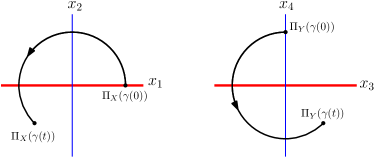
Figure 1: Subgradient curve $\gamma(\cdot)$ generated by $f$ is depicted in black; the set of critical points of $f$ is depicted in red. The picture on the left shows the projection of $\gamma$ onto the coordinate $(x_{1},x_{2})$, while the picture on the right shows the projection of $\gamma$ onto the coordinate $(x_{3},x_{4})$.

It is worthwhile to note that the function $f$ in Theorem 5 trivially satisfies the conclusion of the Morse-Sard theorem, since $f(\mathrm{Crit}(f))=\{0\}$.

3.3 Subgradient sequences without reaching critical points

We next present the final example announced in the introduction. We exhibit a Lipschitz continuous function $f$ such that the subgradient method, which can access $f$ only by querying sugradients, fails to detect critical points in any sense, under any choice of (nonsummable, square summable) steps $\{t_{n}\}_{n\geq 1}$. As the initial attempt at the construction, one may try applying the subgradient method to the function $f$ constructed in Theorem 5, since it has periodic subgradient orbits in continuous time. The difficulty is that when applied to this function, the subgradient iterates (in discrete time) quickly grow unbounded. Therefore, as part of the construction, we will modify the function $f$ from Theorem 5 by exponentially damping its slope.

Theorem 6 (Subgradient method does not detect critical points).

There exists a Lipschitz continuous function $f\colon\mathbb{R}^{4}\to\mathbb{R}$, a subgradient selection $G(X)\in\partial f(X),$ and initial condition $\bar{X}\in\mathbb{R}^{4}$ such that

$$\text{for every sequence\ }\{t_{n}\}_{n}\subset(0,+\infty)\;\text{with}\;\sum_{n\geq 1}t_{n}=+\infty\;\text{and}\;\sum_{n\geq 1}t_{n}^{2}<+\infty$$ (11)

the subgradient algorithm

$$\left\{\begin{aligned} X_{n+1}&=X_{n}-t_{n}G(X_{n})\\ X_{1}&=\bar{X}\end{aligned}\right\}$$ (12)

generates a bounded sequence $\{X_{n}\}_{n\geq 1}$ whose accumulation points do not meet $\mathrm{Crit}(f)$.

Proof. Let us first define the function $\rho:\mathbb{R}^{2}\to\mathbb{R}$ by

$$\rho(x,y)=\exp(-y^{2})\int\limits_{0}^{x}\exp(-\tau^{2})\,d\tau,$$

and notice that

$$\nabla\rho(x,y)=\left(e^{-(x^{2}+y^{2})},\,-2y\cdot\rho(x,y)\right).$$

Then for $\delta>0$ and $M\geq\frac{\delta}{2}(\sqrt{\pi}+1)$, define the function $\phi\colon\mathbb{R}^{2}\to\mathbb{R}$ by

$$\phi(x,y):=\delta\,y\,\rho(x,y)+M\,\int\limits_{0}^{y}\left(\chi_{A}(\tau)-\chi_{A^{c}}(\tau)\right)\,d\tau.$$ (13)

An easy calculation shows that $\phi$ is Lipschitz continuous and its subdifferential is given by

$$\partial\phi(x,y)=\left\{\delta\,y\,e^{-(x^{2}+y^{2})}\right\}\,\times\,\left\{\left(\delta\,(1-2y^{2})\,e^{-y^{2}}\,\int\limits_{0}^{x}e^{-\tau^{2}}d\tau\right)+[-M,M]\right\}.$$ (14)

It follows from (14) that a point $(x,y)\in\mathbb{R}^{2}$ is Clarke critical for $\phi$ if and only if $y=0,$ that is

$$\mathrm{Crit}(\phi)=\mathbb{R}\times\{0\}.$$

We claim that for every $(x,y)\in\mathbb{R}^{2}$, we have

$$g(x,y):=\delta\,e^{-(x^{2}+y^{2})}\,(y,-x)\in\partial\phi(x,y).$$ (15)

To see this, denoting by $\pi_{2}:{\mathbb{R}}^{2}\rightarrow{\mathbb{R}}$ the projection to the second coordinate, we observe:

$$\left|\pi_{2}(g(x,y))-\delta\,(1-2y^{2})\,e^{-y^{2}}\,\int\limits_{0}^{x}e^{-\tau^{2}}d\tau\right| =\delta e^{-y^{2}}\left|(1-2y^{2})\,\int\limits_{0}^{x}e^{-\tau^{2}}d\tau-xe^{-x^{2}}\right|$$

$$\leq\delta e^{-y^{2}}|1-2y^{2}|\cdot\frac{\sqrt{\pi}}{2}+|x|e^{-x^{2}}$$

$$<\delta\cdot\frac{\sqrt{\pi}}{2}+\frac{1}{2}\leq M.$$

Notice that the integral curves of the above vector field

$$(\dot{x},\dot{y})=g(x,y)=\delta\,e^{-(x^{2}+y^{2})}\,(y,-x),$$

are the homocentric cycles $x^{2}+y^{2}=r^{2}$ for any $r\geq 0.$

Consider now applying a subgradient method to $\phi$. Namely, let $\gamma_{n}:=(x_{n},y_{n})$ and consider the subgradient sequence

$$\gamma_{n+1}=\gamma_{n}-t_{n}g_{n},$$ (16)

where we set $g_{n}:=g(x_{n},y_{n})\in\partial f(x_{n},y_{n})$. Then the norms $r_{n}:=\|\gamma_{n}\|$ satisfy

$$\|g_{n}\|=\delta r_{n}e^{-r_{n}^{2}}\leq\frac{\delta}{\sqrt{2e}}.$$ (17)

Since $g_{n}$ is tangent at $\gamma_{n}$ to the homocentric cycle centered at $0$ with radius $r_{n},$ we deduce easily from (16) that the sequence $\{r_{n}\}_{n\geq 1}$ is strictly increasing. On the other hand, by Pythagoras theorem and (17) we deduce:

$$r_{n+1}^{2}\,=\,r_{n}^{2}\,+\,t_{n}^{2}\,\|g_{n}\|^{2}\leq\,r_{n}^{2}\,+\,\left(\frac{\delta^{2}}{2e}\right)t_{n}^{2},$$

and by induction

$$r_{n+1}^{2}\,\leq\,r_{1}^{2}\,+\left(\frac{\delta^{2}}{2e}\right)\sum_{n\geq 1}t_{n}^{2}<+\infty.$$

Therefore, $\{r_{n}\}_{n\geq 1}$ is bounded and the sequence $\gamma_{n}:=(x_{n},y_{n})$ has accumulation points.

The proof is not yet complete, since in principle, the accumulation points of the sequence $(x_{n},y_{n})$ may be critical. To eliminate this possibility, we proceed as in the proof of Theorem 5 by doubling the dimension. Namely, define the function

$$\left\{\begin{array}[c]{l}f\colon\mathbb{R}^{4}\to\mathbb{R}\vspace{0.3cm}\\ f(x,y,z,w)=\phi(x,y)+\phi(z,w)\end{array}\right.,$$ (18)

and observe that $f$ is Lipschitz continuous and equality holds:

$$\mathrm{Crit}(f)=\mathbb{R}\times\{0\}\times\mathbb{R}\times\{0\}.$$

We shall now prescribe a subgradient selection:

$$G(x,y,z,w)=(g(x,y),g(z,w))\in\partial f(x,y,z,w),$$ (19)

where $g(\cdot,\cdot)$ is defined in (15). Let us also prescribe the initial condition

$$X_{1}\equiv\bar{X}=(1,0,0,1)\in\mathbb{R}^{4}.$$

Then (12) generates a bounded sequence

$$X_{n}:=(x_{n},y_{n},z_{n},w_{n})\text{\quad with\quad}G_{n}:=G(X_{n})\in\partial f(X_{n})$$

which splits in ${\mathbb{R}}^{2}\times{\mathbb{R}}^{2}$ as follows:

$$X_{n}=(\gamma_{n},\tilde{\gamma}_{n}),\;G_{n}=(g_{n},\tilde{g}_{n})\in\partial f(X_{n})\text{\quad with\quad}\gamma_{n}:=(x_{n},y_{n})\quad\text{and\quad\ }\tilde{\gamma}_{n}:=(z_{n},w_{n})$$

such that

$$\left\{\begin{array}[c]{c}\gamma_{n+1}=\gamma_{n}-t_{n}g_{n}\\ g_{n}\in\partial\phi(\gamma_{n})\end{array}\right\}\quad\text{and}\quad\text{ }\left\{\begin{array}[c]{c}\tilde{\gamma}_{n+1}=\tilde{\gamma}_{n}-t_{n}\tilde{g}_{n}\\ \tilde{g}_{n}\in\partial\phi(\tilde{\gamma}_{n})\end{array}\right\},$$ (20)

respectively. Thanks to the initial condition, for every $n\geq 1$ the vector $\tilde{\gamma}_{n}$ is a $\frac{\pi}{2}$-rotation of the vector $\gamma_{n}.$ Taking into account this rotational symmetry we deduce that all limit points of $\{X_{n}\}_{n\geq 1}$ lie outside of $\mathrm{Crit}(f)$. $\hfill\Box$

It is worthwhile to note again that the function $f$ in Theorem 6 trivially satisfies the conclusion of the Morse-Sard theorem, since $f(\mathrm{Crit}(f))=\{0\}$.

Acknowledgments. A major part of this work was done during a research visit of the first author to the University of Washington (July 2019). This author thanks the host institute for hospitality. The first author’s research has been supported by the grants CMM-AFB170001, FONDECYT 1171854 (Chile) and PGC2018-097960-B-C22, MICINN (Spain) and ERDF (EU). The research of the second author has been supported by the NSF DMS 1651851 and CCF 1740551 awards.

Aris Daniilidis

DIM–CMM, UMI CNRS 2807
Beauchef 851, FCFM, Universidad de Chile

E-mail: arisd@dim.uchile.cl; URL: http://www.dim.uchile.cl/$\scriptstyle\sim$arisd

Research supported by the grants:
CMM AFB170001, FONDECYT 1171854 (Chile), PGC2018-097960-B-C22 (Spain and EU).

Dmitriy Drusvyatskiy

Department of Mathematics, University of Washington, Seattle, WA 98195

E-mail: ddrusv@uw.edu; URL: www.math.washington.edu/$\scriptstyle\sim$ddrusv

Research supported by the NSF DMS 1651851 and CCF 1740551 awards

 

Appendix: Proof of Lemma 2

We will first need the following lemma, outlining a standard construction of a fat Cantor set. We will impose an extra property, which will play a key role in establishing Lemma 2.

Lemma 7 ($\alpha$-fat Cantor set with attributes).

Fix any $\alpha\in(0,1)$. Then for every interval $I=[a,b]\subset\mathbb{R}$ there exists an $\alpha$-fat Cantor subset $\mathcal{F}_{\alpha}(I)\subset I$, that is, a Cantor-type set of total measure

$$m(\mathcal{F}_{\alpha}(I))=\alpha\,m(I).$$

Moreover, for any $\frac{1}{2}<\lambda<1,$ taking $\alpha>\frac{3\lambda}{2+\lambda}$ we ensure that

$$m(\mathcal{F}_{\alpha}(I)\cap[a,x])\geq\lambda\cdot m([a,x]),\quad\text{for all }x\in[a,b].$$ (21)

Proof. The construction is standard and is sketched for the reader’s convenience. Fix any $\alpha\in(0,1)$. Let us denote $I^{0}=(a,b),$ $\ell_{0}=m(I^{0})=b-a$ and let us set:

$$\delta_{0}:=\left(\frac{1-\alpha}{2}\right)\cdot\ell_{0}>0.$$ (22)

We shall construct the fat-Cantor set by removing, successively, countably many intervals, indexed by a dyadic tree. To this end, we start by removing from our initial set $I^{0}$ the interval

$$\Delta^{0}:=\left[\frac{b+a-\delta_{0}}{2},\frac{b+a+\delta_{0}}{2}\right],$$

that is, an interval of length $\delta_{0}$ centered at $\frac{a+b}{2}$ (the midpoint of $I^{0}$). Then from each of the two remaining intervals $I_{0}^{1}:=(a,\frac{b+a-\delta_{0}}{2})$ and $I_{1}^{1}:=(\frac{b+a+\delta_{0}}{2},b)$ we subtract intervals $\Delta_{0}^{1}$ and $\Delta_{1}^{1}$ of length

$$\delta_{1}:=\frac{1}{2}\cdot\frac{\delta_{0}}{2}$$ (23)

centered at the midpoints of $I_{0}^{1}$ and $I_{1}^{1}$ respectively. Setting

$$m(I_{0}^{1})=m(I_{1}^{1}):=\ell_{1}=\frac{\ell_{0}-\delta_{0}}{2}$$

we observe that

$$\frac{m(\Delta^{0})}{m(I^{0})}=\frac{\delta_{0}}{\ell_{0}}=\frac{1-\alpha}{2}\quad\text{and\quad}\frac{m(\Delta_{i}^{1})}{m(I_{i}^{1})}=\frac{\delta_{1}}{\ell_{1}}=\frac{(\delta_{0}/4)}{(\ell_{0}-\delta_{0})/2}=\frac{1}{2}\left(\frac{1-\alpha}{1+\alpha}\right),\quad\text{for }i\in\{0,1\},$$

and consequently

$$\frac{m(\Delta_{i}^{1})}{m(I_{i}^{1})}=\left(\frac{1}{1+\alpha}\right)\frac{m(\Delta^{0})}{m(I^{0})}\;<\,\frac{m(\Delta^{0})}{m(I^{0})},\quad\text{for }i\in\{0,1\}.$$ (24)

The above relation reveals that in the second step, we subtract a proportionally smaller part of each of the intervals $I_{i}^{1}$, $i\in\{0,1\},$ compared with what we subtract from $I^{0}$ in the first step.
We continue by induction, subtracting at the step $n$ intervals $\Delta_{k}^{n},$ $k\in\{0,1,\ldots,2^{n}-1\},$ of length

$$\delta_{n}=\frac{1}{2}\cdot\frac{\delta_{n-1}}{2}=\frac{1}{2^{n}}\cdot\frac{\delta_{0}}{2^{2}}$$

centered at the midpoints of the intervals $I_{k}^{n}$, where $m(I_{k}^{n})=\ell_{n}=(\ell_{n-1}-\delta_{n-1})/2$, so that for all $k^{\prime}\in\{0,1,\ldots,2^{n-1}-1\}$ and $k\in\{0,1,\ldots,2^{n}-1\}$ we have:

$$\frac{m(\Delta_{k}^{n})}{m(I_{k}^{n})}=\frac{\delta_{n}}{\ell_{n}}=\frac{(\delta_{n-1}/4)}{(\ell_{n-1}-\delta_{n-1})/2}<\frac{\delta_{n-1}}{\ell_{n-1}}=\frac{m(\Delta_{k^{\prime}}^{n})}{m(I_{k}^{n})}.$$ (25)

The above relation says that at the step $n\geq 2$ we remove a proportionally smaller part of each of the intervals $I_{k}^{n}$, $k\in\{0,1,\ldots,2^{n}-1\},$ compared to what we did in the previous step to the intervals $I_{k^{\prime}}^{n}$, $k^{\prime}\in\{0,1,\ldots,2^{n-1}-1\}$.

Let now $\mathcal{F}_{\alpha}(I)$ be the complement of the union of all extracted intervals. Clearly $\mathcal{F}_{\alpha}(I)$ cannot contain any interval (i.e. it is a Cantor-type set), and in view of (22) its total length is

$$m(\mathcal{F}_{\alpha}(I))=m(I)-\left(\delta+2(\frac{1}{2}\cdot\frac{\delta}{2})+2^{2}(\frac{1}{2^{2}}\cdot\frac{\delta}{2^{2}})+\ldots\right)=m(I)-\delta\sum_{n\geq 0}\frac{1}{2^{n}}=\alpha\,m(I).$$

It remains to prove that (21) holds. To this end, we start by treating the case $x\in[a,b]\diagdown\mathcal{F}_{\alpha}(I).$
Let us first assume

$$x\in\Delta^{0}:=\left[\frac{b+a-\delta_{0}}{2},\frac{b+a+\delta_{0}}{2}\right].$$

In this case (which is the less favorable case) we have:

$$m([a,x])\leq\frac{b-a+\delta_{0}}{2}=\frac{\ell_{0}+\delta_{0}}{2}\quad\text{and\quad}m(\mathcal{F}_{\alpha}(I)\cap[a,x])=\frac{m(\mathcal{F}_{\alpha}(I))}{2}=\frac{\alpha\ell_{0}}{2}.$$ (26)

Therefore (21) holds for $\alpha>3\lambda(2+\lambda)^{-1}$.

Assume now that $x\in\Delta_{0}^{1}\cup\Delta_{1}^{1}.$ By construction, using (22), (23) and (24), we deduce that for $i\in\{0,1\},$ the set $\mathcal{F}_{\alpha}(I^{0})\cap I_{i}^{1}$ is an $\alpha_{1}$-fat Cantor set in $I_{i}^{1}$, denoted $\mathcal{F}_{\alpha_{1}}(I_{i}^{1}),$ where $\alpha_{1}$ satisfies:

$$\frac{1-\alpha_{1}}{2}:=\frac{\delta_{1}}{\ell_{1}}=\left(\frac{1}{1+\alpha}\right)\left(\frac{\delta_{0}}{\ell_{0}}\right)=\left(\frac{1}{1+\alpha}\right)\left(\frac{1-\alpha}{2}\right)\quad\text{yielding that }\,\,\alpha_{1}=\frac{2\alpha}{1+\alpha}>\alpha.$$

The above guarantees that for $x\in\Delta_{0}^{1}\subset I_{0}^{1}=\left(a,\frac{b+a-\delta_{0}}{2}\right)$ we have

$$m(\mathcal{F}_{\alpha}(I^{0})\cap[a,x])=m(\mathcal{F}_{\alpha_{1}}(I_{i}^{1})\cap[a,x])\geq\lambda\cdot m([a,x])$$

by the previous step. If now

$$x\in\Delta_{1}^{1}\subset I_{1}^{1}=\left(\frac{b+a+\delta_{0}}{2},b\right)$$

then by (26) and the fact that $\mathcal{F}_{\alpha_{1}}(I_{1}^{1}):=\mathcal{F}_{\alpha}(I^{0})\cap I_{1}^{1}$ is an $\alpha_{1}$-fat Cantor set in $I_{1}^{1}$ with $\alpha_{1}>\alpha$ we deduce:

$$m(\mathcal{F}_{\alpha}(I^{0})\cap[a,x]) =\frac{m(\mathcal{F}_{\alpha}(I))}{2}+m\left(\mathcal{F}_{\alpha_{1}}(I_{1}^{1})\cap\left[\frac{b+a+\delta_{0}}{2},x\right]\right)$$

$$\geq\lambda\cdot\left(m\left(\left[a,\frac{b+a+\delta_{0}}{2}\right]\right)+m\left(\left[\frac{b+a+\delta_{0}}{2},x\right]\right)\right),$$

that is (21) holds. Continuing, we deduce that (21) holds for all $x\in[a,b]\diagdown\mathcal{F}_{\alpha}(I)$.

Let now $x\in\mathcal{F}_{\alpha}(I)$. Then there exists $\{x_{n}\}\subset[a,b]\diagdown\mathcal{F}_{\alpha}(I)$ with $\{x_{n}\}\rightarrow x$. Then by (21) we have

$$m(\mathcal{F}_{\alpha}(I^{0})\cap[a,x_{n}])\geq\lambda\cdot m([a,x_{n}])\quad\text{for all }n\geq 1.$$

The result follows by passing to the limit as $n\to\infty$. The proof is complete. $\hfill\Box$

We are now ready to complete the proof of Lemma 2.

Proof of Lemma 2. Let us fix $\lambda\in(\frac{1}{2},1)$ and choose $\alpha,\theta<1$ (close to $1$) such that

$$\alpha\cdot\theta>\lambda\qquad\text{and}\qquad\alpha>3\lambda(2+\lambda)^{-1}.$$

For any interval $I=[a,b]$, we set

$$I^{+}:=[a,a+\theta(b-a)]\quad\text{and\quad}I^{-}:=[a+\theta(b-a),b]$$

and we define the operators:

• $\mathcal{T}(I):=\mathcal{F}_{\alpha}(I^{+})$ (partial $\alpha$-fat Cantor subset of $I$ of measure $\alpha\cdot\theta\cdot m(I)$), and

• $\mathcal{N}(I)=\mathcal{F}_{\frac{1}{2}}(I^{-})$ (partial $\frac{1}{2}$-fat Cantor subset of $I$ of measure $\frac{1}{2}(1-\theta)m(I)$).

Notice that it is sufficient to construct $A_{0}\subset[0,1]$ (splitting the family of intervals of $(0,1)$) satisfying (5) for $x\in[0,1)$. Indeed, translating the construction by $n$ we obtain $A_{n}\subset[n,n+1)$ and we observe that the set $A=\cup_{n}A_{n}$ has the desired property.

To this end, set $I_{0}=[0,1]$ and consider an enumeration $\{I_{n}\}_{n\geq 1}$ of all strict subintervals $I_{n}:=[p_{n},q_{n}]$ of $[0,1]$ with rational endpoints $p_{n},$ $q_{n}\in\mathbb{Q}$. Set further $T_{0}:=\mathcal{T}(I_{0})$ and $N_{0}:=\mathcal{N}(I_{0})$ and notice that $\left(T_{0}\cup N_{0}\right)$ contains no intervals. Let $I_{1}:=(p_{1},q_{1})$ be the first interval of the above enumeration. Then there exists a subinterval $I_{1}^{\prime}=[p_{1}^{\prime},q_{1}^{\prime}]$ of $I_{1}$ contained in $I_{0}\diagdown\left(T_{0}\cup N_{0}\right)$. We set $T_{1}=\mathcal{T}(I_{1}^{\prime})$ and $N_{1}=\mathcal{N}(I_{1}^{\prime})$ . Similarly, we find a subinterval $I_{2}^{\prime}\subset I_{2}$ contained in

$$I_{0}\diagdown\left[\left(T_{0}\cup T_{1}\right)\cup\left(N_{0}\cup N_{1}\right)\right]$$

and set $T_{2}=\mathcal{T}(I_{2}^{\prime})$ and $N_{2}=\mathcal{N}(I_{2}^{\prime})$ and continue by induction. Then set

$$N=\bigcup_{i=0}^{\infty}N_{i}\quad\text{and}\quad A_{0}=I_{0}\setminus N.$$

It is easily seen that $A_{0}$ splits the family of intervals of $I_{0}=[0,1].$ Let us show that (5) holds.
Let $t\in[0,1]=I_{0}.$ If $t\in I_{0}^{+}=[0,\theta),$ then since $T_{0}=\mathcal{F}_{\alpha}(I_{0}^{+})$ we conclude by Lemma 7 that

$$m(A\cap[0,t])\geq m(T_{0}\cap[0,t])\geq\lambda t.$$

If $t\in I_{0}^{-}=[\theta,1],$ then

$$m(A\cap[0,t])\geq m(T_{0}\cap[0,t])=m(T_{0})=\alpha\cdot\theta>\lambda\geq\lambda t.$$

Therefore, $A_{0}$ satisfies (5) for all $t\in[0,1]$ and consequently, so does the set $A:=\bigcup_{n=-\infty}^{+\infty}(A_{0}+n)$ for all $t>0$. $\hfill\Box$

References

[1]P. Albano and P. Cannarsa,
Singularities of semiconcave functions in Banach spaces.
In Stochastic analysis, control, optimization and applications,
Systems Control Found. Appl., pages 171–190. Birkhäuser Boston, Boston,
MA, 1999.
[2]R. Aron, V. Gurariy, J. Seoane, Lineability and
spaceability of sets of functions on , Proc. Amer. Math.
Soc.133 (2005), 795–803.
[3]M. Benaïm, J. Hofbauer, and S. Sorin,
Stochastic approximations and differential inclusions.
SIAM J. Control Optim.44 (2005), 328–348.
[4]M. Benaïm, J. Hofbauer, and S. Sorin,
Stochastic approximations and differential inclusions. II.
Applications.
Math. Oper. Res., 31 (2006), 673–695.
[5]L. Bernal-Gonzalez, M. Ordonez-Cabrera, Lineability
criteria with applications, J. Funct. Anal.266 (2014), 3997–4025.
[6]L. Bernal-Gonzalez, D. Pellegrino, J.
Seoane-Sepulveda, Linear subsets of nonlinear sets in topological vector
spaces, Bull. Amer. Math. Soc.51 (2014), 71–130.
[7]J. Bolte, A. Daniilidis, A. S. Lewis, M. Shiota,
Clarke subgradients of stratifiable functions, SIAM J. Optim.18 (2007), 556–572.
[8]V. S. Borkar,
Stochastic approximation.
Cambridge University Press, Cambridge; Hindustan Book Agency, New
Delhi, 2008.
A dynamical systems viewpoint.
[9]J. Borwein, W. Moors, X. Wang, Lipschitz functions
with prescribed derivatives and subderivatives, Nonlinear Anal.29 (1997), 53–63.
[10]J. Borwein, X. Wang, Lipschitz functions with
maximal subdifferentials are generic, Proc. Amer. Math. Soc.128 (2000), 3221–3229.
[11]H. Brézis,
Opérateurs maximaux monotones et semi-groupes de contraction
dans des espaces de Hilbert.
North-Holland Math. Stud. 5, North-Holland, Amsterdam, 1973.
[12]R. E. Bruck,