Asymptotically Unbiased Estimation of Physical Observables with Neural Samplers
Abstract
We propose a general framework for the estimation of observables with generative neural samplers focusing on modern deep generative neural networks that provide an exact sampling probability. In this framework, we present asymptotically unbiased estimators for generic observables, including those that explicitly depend on the partition function such as free energy or entropy, and derive corresponding variance estimators. We demonstrate their practical applicability by numerical experiments for the 2d Ising model which highlight the superiority over existing methods. Our approach greatly enhances the applicability of generative neural samplers to real-world physical systems.
pacs:
05.10.Ln, 05.20.−yI Introduction
Monte-Carlo methods are the workhorses of statistical physics and lattice field theories providing insights in strongly correlated systems from first principles Gattringer and Lang (2009); Newman and Barkema (1999a). In spite of their overall success, these approaches come with a number of downsides: Monte-Carlo methods potentially get trapped in local minima that prevent them from exploring the full configuration space Kirkpatrick et al. (1983). Furthermore, they can suffer from large autocorrelation times — in particular close to criticality thus making them very costly in certain regions of the parameter space. In these regions, observables at physical parameter values can often only be extrapolated from simulations at unphysical parameter values. Last but not least, observables that explicitly depend on the partition function, such as free energy and entropy, can only be evaluated up to an overall constant by ”chaining” the results of a considerable number of Monte-Carlo chains Newman and Barkema (1999a); Bishop (2006); Nakajima et al. (2019).
Generative neural samplers (GNSs) are machine learning models which allow sampling from probability distributions learned by using deep neural networks. We refer to Goodfellow et al. (2016) for an accessible overview. GNSs have shown remarkable performance in generating realistic samples capturing complicated probability distributions of real-world data such as images, speech, and text documents. This has inspired the application of GNSs in the context of theoretical physics Torlai and Melko (2016); Morningstar and Melko (2017); Liu et al. (2017); Huang and Wang (2017); Li and Wang (2018); Koch-Janusz and Ringel (2018); Urban and Pawlowski (2018); Zhou et al. (2019); Mustafa et al. (2019); Nicoli et al. (2019); Hu et al. (2019); Yang et al. (2019); Albergo et al. (2019); Wu et al. (2019); Sharir et al. (2019); Noé et al. (2019).
In this work, we focus on a particularly promising subclass of GNSs. Namely, we will consider deep neural networks that allow to sample configurations from the model and also provide the exact probability of the sample . A notable example for this type of GNS are Variational Autoregressive Networks (VANs)Wu et al. (2019), which sample from a PixelCNN Oord et al. (2016) to estimate observables. The main advantage of this class of GNSs is that they can be trained without resorting to Monte-Carlo configurations by minimizing the Kullback–Leibler divergence between the model and a target (Boltzmann) distribution . As a result, they represent a truly complementary approach to existing Monte-Carlo methods.
Observables are often estimated by directly sampling from the GNS and then taking the sample mean. However, as we will discuss in detail, this approach suffers from a mismatch of the sampling distribution and the target distribution . This mismatch is unavoidable since it cannot be expected that the GNS fully captures the underlying physics. This leads to uncontrolled estimates as both the magnitude and the direction of this bias is in general unknown and scales unfavorably with the system size Nicoli et al. (2019).
In this work, we propose a general framework to avoid this serious problem. Our method applies to any GNS with exact sampling probability. Specifically, we will show that it is possible to define asymptotically unbiased estimators for observables along with their corresponding variance estimators. Notably, our method also allows to directly estimate observables that explicitly depend on the partition function, e.g. entropy and free energy. Our proposal therefore greatly enhances the applicability of GNSs to real-world systems.
The paper is organized as follows: In Section II, we will discuss the proposed asymptotically unbiased estimators for observables along with corresponding variance estimators. We illustrate the practical applicability of our approach for the two-dimensional Ising model in Section III, discuss the applicabilty to other GNSs in Section IV and conclude in Section V. Technical details are presented in several appendices.
II Asymptotically Unbiased Estimators
II.1 Generative Neural Samplers with Exact Probability (GNSEP)
We will use a particular subclass of GNSs to model the variational distribution as they can provide the exact probability of configurations and also allow sampling from this distribution . We will henceforth refer to this subclass as generative neural samplers with exact probability (GNSEP). Using these two properties, one can then minimize the inverse Kullback–Leibler divergence between the Boltzmann distribution and the variational distribution without relying on Monte-Carlo configurations for training,
| (1) |
This objective can straightforwardly be optimized using gradient decent since the last summand is an irrelevant constant shift. After the optimization is completed, observables (expectation values of an operator with respect to the Boltzmann distribution ) are then conventionally estimated by the sample mean
| (2) |
using the neural sampler .
Various architectures for generative neural samplers are available. Here, we will briefly review the two most popular ones:
Normalizing Flows (NFs):
Samples from a prior distribution , such as a standard normal, are processed by an invertible neural network . The probability of a sample is then given by
The architecture of is chosen such that the inverse and its Jacobian can easily be computed. Notable examples of normalizing flows include NICEDinh et al. (2015), RealNVPDinh et al. (2017) and GLOWKingma and Dhariwal (2018). First physics applications of this framework have been presented in Noé et al. (2019) in the context of quantum chemistry and subsequently in Albergo et al. (2019) for lattice field theory.
Autoregressive Models (AMs):
In this case, an ordering of the components of is chosen and the conditional distribution is modeled by a neural network. The joint probability is then obtained by multiplying the conditionals
| (3) |
and one can draw samples from by autoregressive sampling from the conditionals. State-of-the-art architectures often use convolutional neural networks (with masked filters to ensure that the conditionals only depend on the previous elements in the ordering). Such convolutional architectures were first proposed in the context of image generation with PixelCNN Oord et al. (2016); Salimans et al. (2017) as most prominent example. In Wu et al. (2019) these methods were first used for statistical physics applications.
A major drawback of using generative neural samplers is that their estimates are A) (often substantially) biased and B) do not come with reliable error estimates, see Figure 1. Both properties are obviously highly undesirable for physics applications. The main reason for this is that the mean (2) is taken over samples drawn from the sampler to estimate expectation values with respect to the Boltzmann distribution . However, it cannot be expected that the sampler perfectly reproduces the target distribution . This discrepancy will therefore necessarily result in a systematic error which is often substantial. Furthermore, in all the cases that we are aware of, this error cannot be reliably estimated.
In order to avoid this serious problem, we propose to use either importance sampling or Markov chain Monte Carlo (MCMC) rejection sampling to obtain asymptotically unbiased estimators. We also derive expressions for the variances of our estimators.
II.2 Sampling Methods
Here we propose two novel estimators that are asymptotically unbiased and are shown to alleviate the serious issues A) and B) mentioned in the previous section.
Neural MCMC (NMCMC) uses the sampler as the proposal distribution for a Markov Chain. Samples are then accepted with probability
| (4) |
We note that the proposal configurations do not depend on the previous elements in the chain. This has two important consequences: Firstly, they can efficiently be sampled in parallel. Secondly, the estimates will typically have very small autocorrelation.
Neural Importance Sampling (NIS) provides an estimator by
| with | (5) |
where for is the importance weight. It is important to stress that we can obtain the configurations by independent identically distributed (iid) sampling from . This is in stark contrast to related reweighting techniques in the context of MCMC sampling Gattringer and Lang (2009).
We assume that the output probabilities of the neural sampler are bounded within for small . In practice, this can easily be ensured by rescaling and shifting the output probability of the model as explained in Appendix B.
It then follows from standard textbook arguments that these two sampling methods provide asymptotically unbiased estimators. For convenience, we briefly recall these arguments in Appendix B.
We note that our asymptotic unbiased sampling methods have the interesting positive side effect that they allow for transfer across parameter space, a property they share with conventional MCMC approaches Newman and Barkema (1999b). For example, we can use a neural sampler trained at inverse temperature to estimate physical observable at a different target temperature , as shown later in Section III. In some cases, this can result in a significant reduction of runtime, as we will demonstrate in Section III.
II.3 Asymptotically Unbiased Estimators
For operators which do not explicitly depend on the partition function, such as internal energy or absolute magnetization , both NIS and NMCMC provide asymptotically unbiased estimators as explained in the last section.
However, generative neural samplers are often also used for operators explicitly involving the partition function . Examples for such quantities include
| (6) | |||
| (7) |
which can be used to estimate the free energy and the entropy respectively. Since the Kullback-Leibler divergence is greater or equal to zero, it follows from the optimization objective (1) that
| (8) |
Therefore, the variational free energy provides an upper bound on the free energy and is thus often used as its estimate. Similarly, one frequently estimates the entropy by simply using the variational distribution instead of . Both estimators however typically come with substantial biases which are hard to quantify. This effect gets particularly pronounced close to the critical temperature.
Crucially, neural importance sampling also provides asymptotically unbiased estimators for by
| with | (9) |
where the partition function is estimated by
| (10) |
In the next section, we will derive the variances of these estimators. Using these results, the errors of such observables can systematically be assessed.
II.4 Variance Estimators
In the following, we focus on observables of the form
| (11) |
that include the estimators for internal energy, magnetization but most notably also for free energy (6) and entropy (7). As just mentioned, expectation values of these operators can be estimated using (9).
Let us assume that is differentiable at the true value of the partition function . Then, as shown in Appendix C, the variance of the estimator for large is given by
| (12) |
where
| (13) |
Note that can be estimated by
| (14) |
and can be estimated by (10), respectively.
For operators with , it is well-known Kong (1992) that Eq. (12) reduces to
| (15) |
where we have defined the effective sampling size
| (16) |
Note that the effective sampling size does not depend on the particular form of . It is however important to stress that for observables with , the error cannot be estimated in terms of effective sampling size but one has to use (12). While this expression is more lengthy, it can be easily estimated. Therefore, neural importance sampling allows us to reliably estimate the variances of physical observables — in particular observables with explicit dependence on the partition function. This is in stark contrast to the usual GNS approach.
It is also worth stressing that MCMC sampling does not allow to directly estimate those observables which explicitly involve the partition function. For completeness, we also note that a similar well-known effective sampling size can be defined for MCMC
| (17) |
where is the integrated auto-correlation time of the operator , see Wolff et al. (2004); Gattringer and Lang (2009) for more details.
III Numerical Results
We will now demonstrate the effectiveness of our method on the example of the two-dimensional Ising model with vanishing external magnetic field. This model has an exact solution and therefore provides us with a ground truth to compare to. The Hamiltonian of the Ising model is given by
| (18) |
where is the coupling constant and the sum runs over all neighbouring pairs of lattice sites. The corresponding Boltzmann distribution is then given by
| (19) |
with partition function . For simplicity, we will absorb the coupling constant in in the following. Here, we will only consider the ferromagnetic case for which and the model undergoes a second-order phase transition at in the infinite volume limit.
In addition to the exact solution by Onsager for the infinite volume case Onsager (1944), there also exists an analytical solution for finite lattices Ferdinand and Fisher (1969), which we review in Appendix A and use for reference values. An exact partition function for the case of vanishing magnetic field is not enough to derive expressions for some observables, such as magnetization. For these observables, we obtain reference values by using the Wolff MCMC clustering algorithm Wolff (1989).
III.1 Unbiased Estimators for the Ising Model
For discrete sampling spaces, autoregressive algorithms are the preferred choice as normalizing flows are designed for continuous ones 111However, Tran et al. (2019); Hoogeboom et al. (2019) present a recent attempt to apply normalizing flows to discrete sampling spaces.. It is nonetheless important to stress that our proposed method applies irrespective of the particular choice for the sampler.
We use the standard VAN architecture for the GNS. For training, we closely follow the procedure described in the original publication Wu et al. (2019). More detailed information about hyperparameter choices can be found in Appendix D. We use VANs, trained for a lattice at various temperatures around the critical point, to estimate a number of observables. The errors for neural importance sampling are determined as explained in Section II.4. For Wolff and Neural MCMC, we estimate the autocorrelation time as described in Wolff et al. (2004).
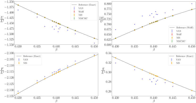
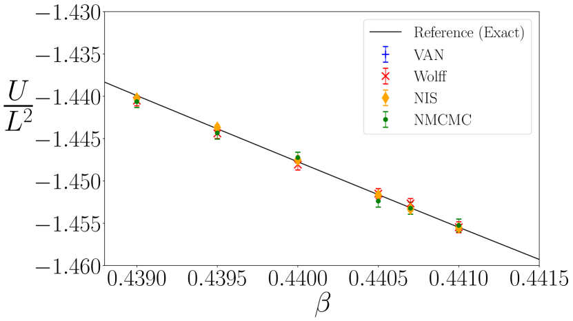
Figure 1 summarizes the main results of our experiments in terms of estimates for internal energy, absolute magnetization, entropy and free energy around the critical regime. NMCMC and NIS agree with the reference values while VAN deviates significantly. We note that this effect is also present for observables with explicit dependence on the partition function, i.e. for entropy and free energy.
All estimates in Figure 1 deviate from the reference value in the same direction. Whereas this is expected for the free energy (for which the true value is a lower bound) also for the other observables the trained GNSs seem to favor a certain direction of approaching the true value. However, as we show in Appendix E, this trend holds only on average and is not a systematic effect.
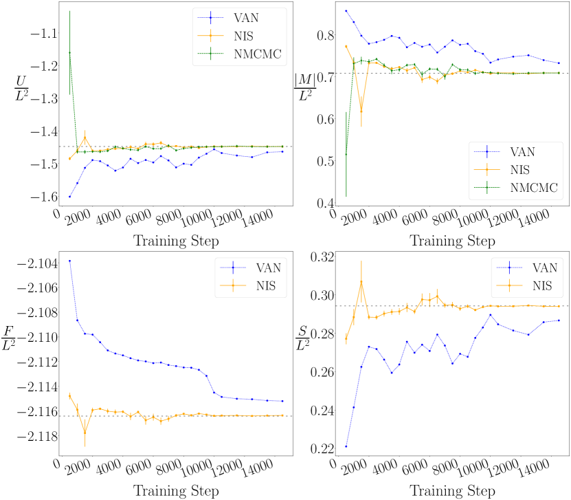
In Figure 3, we track the evolution of the estimates for the four observables under consideration during training. This figure clearly demonstrates that our proposed method leads to accurate predictions even at earlier stages of the training process. This is particularly important because the overall runtime for GNS estimates is heavily dominated by the training.
Table 1 summarizes results for lattice. For this larger lattice, the systematic error of VAN is even more pronounced and the estimated values do not even qualitatively agree with the reference values. Our modified sampling techniques, on the other hand, lead to fully compatible results.
| Lattice | Sampler | ||||
|---|---|---|---|---|---|
| (24x24) | VAN | -1.5058 (0.0001) | 0.7829 (0.0001) | 0.26505 (0.00004) | -2.107250 (0.000001) |
| NIS | -1.43 (0.02) | 0.67 (0.03) | 0.299 (0.007) | -2.1128 (0.0008) | |
| NMCMC | -1.448 (0.007) | 0.68 (0.04) | - | - | |
| Reference | -1.44025 | 0.6777 (0.0006) | 0.29611 | -2.11215 | |
| (16x16) | VAN | -1.4764 (0.0002) | 0.7478 (0.0002) | 0.28081 (0.00007) | -2.11363 (0.00001) |
| NIS | -1.4533 (0.0003) | 0.71363 (0.00004) | 0.2917 (0.0002) | -2.11529 (0.00001) | |
| NMCMC | -1.4532 (0.0007) | 0.714 (0.001) | - | - | |
| Reference | -1.4532 | 0.7133 (0.0008) | 0.29181 | -2.11531 |

Lastly, our proposed methods allow for transfer across parameter space, as explained in Section II.2. In Figure 6, we summarize a few transfer runs. We performed a full training procedure for each value of shown in Figure 6. The trained samplers were then used to estimate observables at (i.e. not at the training temperature ). All predicted values agree with the reference within error bars. As the difference between model’s temperature and target increases, the variance grows as well — as was to be expected. In practice, this limits the difference between model and target inverse temperature. Nevertheless, we can use models trained at a single value to predict other values in a non-trivial neighbourhood of the model . This allows to more finely probe parameter space at only minimal additional computational costs.

III.2 Neural MCMC
NMCMC obtains a proposal configuration by independent and identically distributed sampling from the sampler . This can result in a significantly reduced integrated autocorrelation time for the observables . For this reduction, it is not required to perfectly train the sampler. It is however required that the sampler is sufficiently well-trained such that the proposal configuration is accepted with relatively high probability, as illustrated in Figure 4. Table 2 demonstrates a significant reduction in integrated autocorrelation , as defined in (17), for two observables at on a lattice.
| Observable | Metropolis | NMCMC |
|---|---|---|
| 4.0415 | 0.8317 | |
| 7.8510 | 1.3331 |
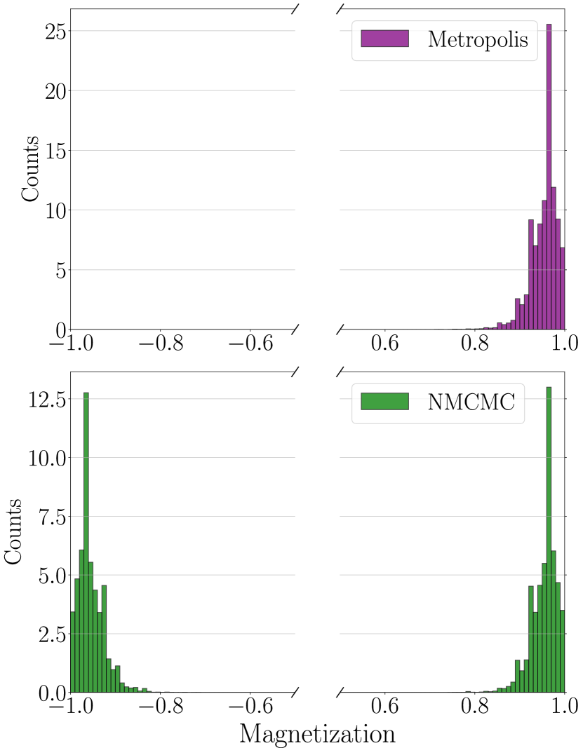
In NMCMC, the proposal configuration is independent of the previous configuration in the chain. This is in stark contrast to the Metropolis algorithm for which the proposal configuration is obtained by a local update of the previous configuration. As a result, NMCMC is less likely to stay confined in (the neighbourhood of) an energy minimum of the configuration space. This is demonstrated in Figure 5 which shows the magnetization histograms for Metropolis and Neural MCMC. Since the Ising model has a discrete -symmetry, we expect a two-moded distribution. In constrast to the Metropolis algorithm, NMCMC indeed shows such a behaviour.
IV Applicability to Other Samplers
We note that our approach can in parts be applied to other generative models. Table 3 summarizes the applicability of neural MCMC (NMCMC) sampling and neural importance sampling (NIS). Namely, when the employed GNS provides an unnormalized sampling probability, i.e., the exact probability multiplied by a constant, then NMCMC and NIS can again correct the learned sampler leading to asymptotically unbiased estimators. However, the applicability is limited to the observables that do not explicitly depend on the partition function, i.e., in Eq. (11).
If the employed GNS allows us to approximate the (normalized or unnormalized) sampling probability, one can apply our approach by using the approximate probability for . The bias can then be reduced if the gap between the target distribution and the sampling distribution is larger than the approximation error to the sampling probability. However, then the estimator may not be asymptotically unbiased.
In summary, our method can be applied broadly to a variety of machine learning models and therefore does not depend on the particular choice of the sampler. Depending on the physical system, a particular architecture may be preferable. For example, whether an autoregressive model or a normalizing flow is the best machine learning tool to use, depends on how the sampling space looks like. The former requires a discrete sampling space, thus being a particularly good match for discrete systems, such as spin chains; the latter finds its applicability in the context of continuous systems, such as lattice field theories. As shown in Table 3, applying our method to these models provides asymptotically unbiased estimators.
V Conclusion and Outlook
In this work, we presented a novel approach for the unbiased estimation of observables with well-defined variance estimates from generative neural samplers that provides the exact sampling probability (GNSEP). Most notably, this includes also observables that explicitly depend on the partition function such as free energy or entropy. The practical applicability of the approach is demonstrated for the two-dimensional Ising model, stressing the importance of unbiased estimators compared to biased estimators from the literature.
In summary, the methods proposed in this paper not only lead to theoretical guarantees but are also of great practical relevance. They are applicable for a large class of generative samplers, easy to implement, and often lead to a significant reduction in runtime. We therefore firmly believe that they will play a crucial role in the promising application of generative models to challenging problems of theoretical physics.
| Accessible sampling probability | NMCMC, NIS() | NIS() | GNSs | Application in Physics |
|---|---|---|---|---|
| none | X | X | GAN | Zhou et al. (2019); Urban and Pawlowski (2018) |
| approximate, unnormalized | (✓) | X | RBM | Carleo and Troyer (2017); Morningstar and Melko (2017) |
| approximate, normalized | (✓) | (✓) | VAE | Cristoforetti et al. (2019) |
| exact, unnormalized | ✓ | X | – | – |
| exact, normalized | ✓ | ✓ | AM, NF | Wu et al. (2019); Noé et al. (2019); Albergo et al. (2019) |
Acknowledgements.
This work was supported by the German Ministry for Education and Research as Berlin Big Data Center (01IS18025A) and Berlin Center for Machine Learning (01IS18037I). This work is also supported by the Information & Communications Technology Planning & Evaluation (IITP) grant funded by the Korea government (No. 2017-0-001779) and by the DFG (EXC 2046/1, Project-ID 390685689). Part of this research was performed while one of the authors was visiting the Institute for Pure and Applied Mathematics (IPAM), which is supported by the National Science Foundation (Grant No. DMS-1440415). The authors would like to acknowledge valuable comments by Frank Noe and Alex Tkatchenko to an earlier version of the manuscript.Appendix A Partition function of the finite-size Ising model
In this appendix, we review the exact solution for the partition function of the finite-size Ising model Ferdinand and Fisher (1969). For an lattice, the partition function is given by
| (20) |
where we have used the definitions
| (21) |
with the coefficients
| for | (22) | ||||
and . From this expression for the partition function, one can easily obtain analytical expressions for the free energy and entropy.
Appendix B Proof of asymptotic Unbiasedness
In this section, we will give a review of the relevant arguments establishing that the NIS and NMCMC estimators are asymptotically unbiased.
For reasons that will become obvious soon, it is advantageous to re-interpret the original network output as the probability by the following mapping:
| (23) |
Due to the rescaling discussed above, we can assume that the support of the sampling distribution contains the support of the target distribution . This property is ensured since the sampler takes values in .
B.1 Neural Importance Sampling
Importance sampling with respect to , i.e.
| (24) |
is an asymptotically unbiased estimator of the expectation value because
| (25) |
where . The partition function can be similarly determined
| (26) |
Combining the previous equations, we obtain
| with | (27) |
B.2 Neural MCMC
The sampler can be used as a trial distribution for a Markov-Chain which uses the following acceptance probability in its Metropolis step
| (28) |
This fulfills the detailed balance condition
| (29) |
because the total transition probability is given by and therefore
| (30) |
where we have used the fact that the min operator is symmetric and that all factors are strictly positive. The latter property is ensured by the fact that .
Appendix C Variance Estimators
| Observable | Estimated Std | Sample Std |
|---|---|---|
| Entropy | 0.00023 | 0.00025 |
| Free En. | 0.00002 | 0.00002 |
As explained in the main text, we estimate observables of the form
| (31) |
by the samples with using
| (32) |
By the definition of , see (10), this is equivalent to
| (33) |
Let
| (34) |
Then, the central limit theorem implies that
| (35) |
where
| (36) |
Appendix D Experimental Details
In this appendix, we provide an overview of the setup used for the experiments presented in this manuscript.
D.1 Model Training
Unless reported differently, all the models were trained for a lattice for a total of steps. The model trained on a lattice required steps until convergence. Our model use the VAN architecture with residual connections (see Wu et al. (2019) for details on this architecture). The networks are six convolutional layers deep (with a half-kernel size of three) and has a width size of 64. A batch size of and a learning rate of were chosen. No learning rate schedulers were deployed in our training. For each model, we applied -annealing to the target using the following annealing schedule
| (40) |
where is the total number of training steps. We summarize the used setup in Table 5. Training a sampler for a and lattices takes respectively and hours of computing time on three Tesla P100 GPUs with 16GB VRAM. As specified before, the former lattice required ten thousands steps of training to converge whereas the latter required fifteen thousands.
| Sampler | Depth | Width | Batch | lr | Steps | Ann. |
|---|---|---|---|---|---|---|
| PixelCNN | 6 | 64 | 0.998 |
| Obs | Model 1 | Model 2 | Model 3 | Model 4 | Model 5 |
|---|---|---|---|---|---|
| -1.5407 | -1.5461 | -1.5364 | -1.5438 | -1.5421 | |
| 0.8089 | 0.8114 | 0.8059 | 0.8098 | 0.8070 | |
| 0.258889 | 0.260271 | 0.257843 | 0.262209 | 0.261478 |
D.2 Neural Monte Carlo and Neural Important Sampling
In Neural MCMC, we use a chain of k steps. Conversely to standard MCMC methods, such as Metropolis, no equilibrium steps are required since we sample from an already trained proposal distribution. In Neural Importance Sampling, batches of 1000 samples are drawn 500 times. Both sampling methods were performed on a Tesla P100 GPU and their runtime is approximately an hour in the case of a .
Appendix E Direction of Bias
In this appendix, we demonstrate that the direction of the bias depends on the random initialization of the network. In order to illustrate this fact, we trained five models at for a 88 lattice using the same hyperparameter setup. We compare the estimate of the energy with an exact reference value of . Table 6 summarizes the results. Values which overestimate the ground truth are in bold. This shows that the trend of under- or overestimating, observed from Figure 1, holds only on average and is not a systematic effect.
References
- Gattringer and Lang (2009) C. Gattringer and C. Lang, Quantum chromodynamics on the lattice: an introductory presentation, Vol. 788 (Springer, 2009).
- Newman and Barkema (1999a) M. Newman and G. Barkema, Monte carlo methods in statistical physics (Oxford University Press, 1999).
- Kirkpatrick et al. (1983) S. Kirkpatrick, C. D. Gelatt, and M. P. Vecchi, Science 220, 671 (1983).
- Bishop (2006) C. M. Bishop, Pattern recognition and machine learning (springer, 2006).
- Nakajima et al. (2019) S. Nakajima, K. Watanabe, and M. Sugiyama, Variational Bayesian Learning Theory (Cambridge University Press, 2019).
- Goodfellow et al. (2016) I. Goodfellow, Y. Bengio, and A. Courville, Deep learning (MIT press, 2016).
- Torlai and Melko (2016) G. Torlai and R. G. Melko, Phys. Rev. B 94, 165134 (2016), arXiv:1606.02718 [cond-mat.stat-mech] .
- Morningstar and Melko (2017) A. Morningstar and R. G. Melko, Journal of Machine Learning Research 18, 163:1 (2017), arXiv:1708.04622 [cond-mat.dis-nn] .
- Liu et al. (2017) Z. Liu, S. P. Rodrigues, and W. Cai, (2017), arXiv:1710.04987 [cond-mat.dis-nn] .
- Huang and Wang (2017) L. Huang and L. Wang, Physical Review B 95, 035105 (2017).
- Li and Wang (2018) S.-H. Li and L. Wang, Physical Review Letters 121, 260601 (2018).
- Koch-Janusz and Ringel (2018) M. Koch-Janusz and Z. Ringel, Nature Physics 14, 578 (2018).
- Urban and Pawlowski (2018) J. M. Urban and J. M. Pawlowski, (2018), arXiv:1811.03533 [hep-lat] .
- Zhou et al. (2019) K. Zhou, G. Endrődi, L.-G. Pang, and H. Stöcker, Physical Review D 100, 011501 (2019).
- Mustafa et al. (2019) M. Mustafa, D. Bard, W. Bhimji, Z. Lukić, R. Al-Rfou, and J. M. Kratochvil, Computational Astrophysics and Cosmology 6, 1 (2019).
- Nicoli et al. (2019) K. Nicoli, P. Kessel, N. Strodthoff, W. Samek, K.-R. Müller, and S. Nakajima, (2019), arXiv:1903.11048 [cond-mat.stat-mech] .
- Hu et al. (2019) H.-Y. Hu, S.-H. Li, L. Wang, and Y.-Z. You, (2019), arXiv:1903.00804 [cond-mat.dis-nn] .
- Yang et al. (2019) L. Yang, Z. Leng, G. Yu, A. Patel, W.-J. Hu, and H. Pu, (2019), arXiv:1905.10730 [cond-mat.str-el] .
- Albergo et al. (2019) M. S. Albergo, G. Kanwar, and P. E. Shanahan, Phys. Rev. D100, 034515 (2019), arXiv:1904.12072 [hep-lat] .
- Wu et al. (2019) D. Wu, L. Wang, and P. Zhang, Physical Review Letters 122, 080602 (2019).
- Sharir et al. (2019) O. Sharir, Y. Levine, N. Wies, G. Carleo, and A. Shashua, (2019), arXiv:1902.04057 [cond-mat.dis-nn] .
- Noé et al. (2019) F. Noé, S. Olsson, J. Köhler, and H. Wu, Science 365 (2019).
- Oord et al. (2016) A. V. Oord, N. Kalchbrenner, and K. Kavukcuoglu, in ICML, Vol. 48 (2016) pp. 1747–1756, arXiv:1601.06759 [cs.CV] .
- Dinh et al. (2015) L. Dinh, D. Krueger, and Y. Bengio, in ICLR Workshop (2015) arXiv:1410.8516 [cs.LG] .
- Dinh et al. (2017) L. Dinh, J. Sohl-Dickstein, and S. Bengio, in ICLR (2017) arXiv:1605.08803 [cs.LG] .
- Kingma and Dhariwal (2018) D. P. Kingma and P. Dhariwal, in NIPS (2018) pp. 10215–10224, arXiv:1807.03039 [stat.ML] .
- Salimans et al. (2017) T. Salimans, A. Karpathy, X. Chen, and D. P. Kingma, in ICLR, Vol. 33 (2017) arXiv:1701.05517 [cs.LG] .
- Newman and Barkema (1999b) M. Newman and G. Barkema, in Monte carlo methods in statistical physics (Oxford University Press, New York, USA, 1999) Chap. 8, pp. 211–216.
- Kong (1992) A. Kong, University of Chicago, Dept. of Statistics, Tech. Rep 348 (1992).
- Wolff et al. (2004) U. Wolff, A. Collaboration, et al., Computer Physics Communications 156, 143 (2004).
- Onsager (1944) L. Onsager, Physical Review 65, 117 (1944).
- Ferdinand and Fisher (1969) A. E. Ferdinand and M. E. Fisher, Physical Review 185, 832 (1969).
- Wolff (1989) U. Wolff, Physics Letters B 228, 379 (1989).
- Note (1) However, Tran et al. (2019); Hoogeboom et al. (2019) present a recent attempt to apply normalizing flows to discrete sampling spaces.
- Carleo and Troyer (2017) G. Carleo and M. Troyer, Science 355, 602 (2017).
- Cristoforetti et al. (2019) M. Cristoforetti, G. Jurman, A. I. Nardelli, and C. Furlanello, (2019), arXiv:1705.09524 [hep-lat] .
- Tran et al. (2019) D. Tran, K. Vafa, K. K. Agrawal, L. Dinh, and B. Poole, in ICLR Workshop (2019) arXiv:1905.10347 [cs.LG] .
- Hoogeboom et al. (2019) E. Hoogeboom, J. W. Peters, R. v. d. Berg, and M. Welling, (2019), arXiv:1905.07376 [cs.LG] .