TUM-HEP 1233/19

Contrast data mining for the MSSM from strings

Erik Parr and Patrick K.S. Vaudrevange

Physik Department T75, Technische Universität München,
James–Franck–Straße 1, 85748 Garching, Germany

We apply techniques from data mining to the heterotic orbifold landscape in order to identify new MSSM-like string models. To do so, so-called contrast patterns are uncovered that help to distinguish between areas in the landscape that contain MSSM-like models and the rest of the landscape. First, we develop these patterns in the well-known $\mathbbm{Z}_{6}$-II orbifold geometry and then we generalize them to all other $\mathbbm{Z}_{N}$ orbifold geometries. Our contrast patterns have a clear physical interpretation and are easy to check for a given string model. Hence, they can be used to scale down the potentially interesting area in the landscape, which significantly enhances the search for MSSM-like models. Thus, by deploying the knowledge gain from contrast mining into a new search algorithm we create many novel MSSM-like models, especially in corners of the landscape that were hardly accessible by the conventional search algorithm, for example, MSSM-like $\mathbbm{Z}_{6}$-II models with $\Delta(54)$ flavor symmetry.

1 Introduction

String theory is a promising candidate for a UV-complete theory of quantum gravity. However, to proof its usefulness it has to incorporate the standard model (SM) or its supersymmetric extension (the MSSM) as a low-energy limit. Thus, one of the main tasks of string phenomenology is to find a string model that is consistent with all experimental and observational data – or, at least, that comes close to the MSSM, i.e. a model that is MSSM-like. This task is very difficult, mainly due to two reasons: (i) String theory predicts extra spatial dimensions. Hence, the connection between string theory and the MSSM must be related to the way how the extra dimensions are compactified. However, the number of different compactifications is huge [1, 2], giving rise to the so-called string landscape of effective 4D theories originating from string theory. (ii) String theory is very predictive because after specifying the compactification the effective 4D theory, including all symmetries, particles and couplings, is completely fixed.

In the case of the ten-dimensional $\mathrm{E}_{8}\times\mathrm{E}_{8}$ heterotic string we have to compactify six dimensions. To do so, we choose six-dimensional toroidal orbifolds [3, 4] as they allow for a world-sheet formulation of string theory instead of a supergravity approximation, see e.g. [5, 6, 7, 8, 9, 10, 11, 12, 13, 14, 15] for other schemes. Then, the conventional approach to search for MSSM-like string models from heterotic orbifolds is given by a random scan in the landscape [16, 17, 18] or in fertile islands that can be identified by certain patterns, like local GUTs [19, 20, 21]. In this paper, we show that the approach of defining fertile islands can be generalized by applying machine learning techniques to the string landscape [22, 23, 24, 25], see also [26, 27, 28, 29, 30, 31, 32, 33]. A first hint towards such a generalization was observed in ref. [34]: a neural network was able to identify additional patterns and to cluster the models of the heterotic orbifold landscape according to them. Surprisingly, MSSM-like models turned out to be localized close to each other on fertile islands, even though the neural network did not know whether a given model is MSSM-like or not, denoted by MSSM-like.

In this paper we propose and demonstrate a new search strategy for MSSM-like models based on additional patterns that is superior by orders of magnitude. This search is developed from the knowledge gained by analyzing the heterotic orbifold landscape with tools from data mining. Data mining has been developed for the purpose to prepare, visualize and explore huge databases. Hence, the suitability of data mining to the string landscape is obvious. In particular, we apply a special setup called contrast data mining to the heterotic orbifold landscape. The basic idea of contrast data mining is to identify so-called contrast patterns that allow us to focus our search on those areas in the landscape where the MSSM-like models reside. Our contrast patterns have a clear physical interpretation: they are given by the number of unbroken roots in the hidden $\mathrm{E}_{8}$ factor [9, 35] and the numbers of various bulk matter fields.

This paper is structured as follows: In section 2 we review the conventional search algorithm for MSSM-like models in the heterotic orbifold landscape. Then, we improve this algorithm using traditional methods: first, we take the Weyl symmetry into account and, secondly, in section 3 we include phenomenological constraints. These improvements already reduce the number of models that have to be scanned by the search algorithm in the test case of the $\mathbbm{Z}_{6}$-II orbifold geometry. Afterwards, in section 4 we apply data mining techniques to our $\mathbbm{Z}_{6}$-II dataset. Doing so, we can identify contrast patterns that help to distinguish between areas in the landscape that contain MSSM-like models and others. We implement these contrast patterns into our search algorithm and show that we can easily construct many new MSSM-like $\mathbbm{Z}_{6}$-II models – a fact that might be surprising given the extensive searches done especially in this orbifold geometry. Remarkably, we can identify two MSSM-like $\mathbbm{Z}_{6}$-II models with $\Delta(54)$ flavor symmetry (related to a vanishing Wilson line of order three), see section 5. Thereafter, our contrast patterns are successfully extended to all $\mathbbm{Z}_{N}$ orbifold geometries in section 6, where table 8 summarizes our results, see also [36]. Finally, in section 7 we conclude.

vector	order $N_{k}$	additional constraint
$V_{1}$	6
$V_{2}$	1	not present, i.e. $V_{2}=(0^{16})$
$W_{1}$	1	$W_{1}=(0^{16})$
$W_{2}$	1	$W_{2}=(0^{16})$
$W_{3}$	3	$W_{3}=W_{4}$
$W_{4}$	3
$W_{5}$	2
$W_{6}$	2

Table 1: Table of geometrical constraints for shift vectors and Wilson lines in the case of the $\mathbbm{Z}_{6}$-II orbifold geometry.

2 Searching the heterotic orbifold landscape

An orbifold compactification [3, 4] is specified by a six-dimensional orbifold geometry $\mathbbm{O}$ and a gauge embedding that acts on the sixteen gauge degrees of freedom of the heterotic string. While there exist only 138 orbifold geometries with Abelian point group (i.e. $\mathbbm{Z}_{N_{1}}$ or $\mathbbm{Z}_{N_{1}}\times\mathbbm{Z}_{N_{2}}$) and $\mathcal{N}=1$ supersymmetry [37], the true size of the heterotic orbifold landscape unfolds if we take the number of inequivalent gauge embeddings into account. For a general $\mathbbm{Z}_{N_{1}}\times\mathbbm{Z}_{N_{2}}$ orbifold, a gauge embedding is given by two shift vectors, $V_{1}$ and $V_{2}$, and six Wilson lines, $W_{1}$ to $W_{6}$, corresponding to the six compactified directions. In this paper we concentrate on the $\mathrm{E}_{8}\times\mathrm{E}_{8}$ heterotic string, which implies that each vector can be split into two eight-dimensional vectors. For example, the sixteen-dimensional shift vector $V_{1}$ consists of the eight-dimensional vectors $V^{(1)}_{1}$ and $V^{(2)}_{1}$, which act on the first and second $\mathrm{E}_{8}$ factor, respectively. Altogether a gauge embedding is determined by a gauge embedding matrix

$$M~{}=~{}\begin{pmatrix}V^{(1)}_{1}&V^{(2)}_{1}\\ V^{(1)}_{2}&V^{(2)}_{2}\\ W^{(1)}_{1}&W^{(2)}_{1}\\ W^{(1)}_{2}&W^{(2)}_{2}\\ W^{(1)}_{3}&W^{(2)}_{3}\\ W^{(1)}_{4}&W^{(2)}_{4}\\ W^{(1)}_{5}&W^{(2)}_{5}\\ W^{(1)}_{6}&W^{(2)}_{6}\\ \end{pmatrix}\;,$$ (1)

where we denote the vector in the $k$-th line by $M_{k}$ for $k=1,\ldots,8$ and split it into two parts $M_{k}^{(\alpha)}$ for $\alpha=1,2$ corresponding to the two $\mathrm{E}_{8}$ factors, for example, $M_{3}=W_{1}=(W^{(1)}_{1},W^{(2)}_{1})$ for the first Wilson line $W_{1}$. Depending on the orbifold geometry, shift vectors and Wilson lines are subject to geometrical constraints that, for example, fix the order of the shift vector $V_{1}$ to $N$ for a $\mathbbm{Z}_{N}$ orbifold geometry, see e.g. ref. [38]. To be more specific and as we will mainly work with the so-called $\mathbbm{Z}_{6}$-II $(1,1)$ orbifold geometry (using the nomenclature from ref. [37], abbreviated as $\mathbbm{Z}_{6}$-II in the following), we summarize the geometrical constraints on the shift vectors and Wilson lines for the $\mathbbm{Z}_{6}$-II orbifold geometry in table 1.

In general, there are two ways to expand a sixteen-dimensional shift vector or Wilson line naturally: either in terms of the simple roots $\alpha_{I}$ of $\mathrm{E}_{8}\times\mathrm{E}_{8}$ or in terms of the dual simple roots $\alpha^{*}_{I}$, $I=1,\ldots,16$, where $\alpha^{*}_{I}\cdot\alpha_{J}=\delta_{IJ}$. Both choices give a basis of the (self-dual) root lattice $\Lambda_{\mathrm{E}_{8}\times\mathrm{E}_{8}}$ of $\mathrm{E}_{8}\times\mathrm{E}_{8}$. For later convenience (see section 2.3) we decide to expand the vectors in terms of the dual basis, i.e. we parameterize the vectors $M_{k}$ in the gauge embedding matrix $M$ as

$$M_{k}~{}=~{}\dfrac{1}{N_{k}}\sum_{I=1}^{16}\ d_{k\,I}\ \alpha^{*}_{I}\;.$$ (2)

Here, $N_{k}$ defines the order of the shift vector or Wilson line and $d_{k\,I}\in\mathbb{Z}$ for $k=1,\ldots,8$ and $I=1,\ldots,16$ are integers. Consequently, a gauge embedding matrix $M$ corresponds to a point in $d\in\mathbbm{Z}^{128}$ since $d_{k\,I}$ has $8\times 16=128$ components. Note that this construction eq. (2) inherently ensures the correct order of the respective vector. In detail, for all vectors $k=1,\ldots,8$ we have

$$N_{k}\,M_{k}~{}\in~{}\Lambda_{\mathrm{E}_{8}\times\mathrm{E}_{8}}\;.$$ (3)

2.1 Conditions from modular invariance

In order to obtain consistent string compactifications we have to impose conditions from modular invariance of the one-loop string partition function on the gauge embedding matrix $M$. These conditions read [39]

$$N_{1}\,\left(V_{1}^{2}-v_{1}^{2}\right) = 0\mod 2\;,$$ (4a)

$$N_{2}\,\left(V_{2}^{2}-v_{2}^{2}\right) = 0\mod 2\;,$$ (4b)

$$\mathrm{gcd}(N_{1},N_{2})\,\left(V_{1}\cdot V_{2}-v_{1}\cdot v_{2}\right) = 0\mod 2\;,$$ (4c)

$$\mathrm{gcd}(N_{i+2},N_{1})\,\left(W_{i}\cdot V_{1}\right) = 0\mod 2\;,$$ (4d)

$$\mathrm{gcd}(N_{i+2},N_{2})\,\left(W_{i}\cdot V_{2}\right) = 0\mod 2\;,$$ (4e)

$$N_{i+2}\,\left(W_{i}^{2}\right) = 0\mod 2\;,$$ (4f)

$$\mathrm{gcd}(N_{i+2},N_{j+2})\,\left(W_{i}\cdot W_{j}\right) = 0\mod 2\quad(i\neq j)\;,$$ (4g)

for $i,j=1,\ldots,6$ and where $v_{1}$ and $v_{2}$ denote the so-called twist vectors. They encode the geometrical rotation angles of a general $\mathbbm{Z}_{N_{1}}\times\mathbbm{Z}_{N_{2}}$ orbifold geometry, while for $\mathbbm{Z}_{N_{1}}$ orbifolds the twist $v_{2}=(0^{4})$ is not present. In addition, the gcd in eq. (4) denotes the greatest common divisor. These conditions are very restrictive and already forbid a huge fraction of points in the space $\mathbbm{Z}^{128}$ corresponding to eq. (2). The only reasonable way to create a consistent gauge embedding matrix $M$ is by successively creating shift vectors and Wilson lines step-by-step and checking each time if the relevant conditions from eqs. (4) are fulfilled for those combinations of shift vectors and Wilson lines that have been chosen so far, see figure 1.

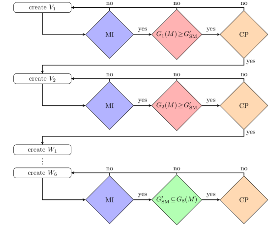
Figure 1: Flowchart of the construction of shift vectors and Wilson lines, starting with the shift vector $V_{1}$ at step $n=1$ and ending with the Wilson line $W_{6}$ at step $n=8$. At each step $n=1,\ldots,8$, the vector $M_{n}$ is chosen randomly and the corresponding modular invariance (MI) conditions are tested. If the vector passes this test, two additional conditions are applied:
(i) As discussed in section 3.1 the gauge group $G_{n}(M)$ is computed using the already chosen vectors $M_{k}$ for $k=1,\ldots,n$. If $G_{n}(M)$ satisfies a necessary condition to host the non-Abelian gauge group factors $G_{\mathrm{SM}}^{\prime}=\mathrm{SU}(3)\times\mathrm{SU}(2)$ of the SM in the first $\mathrm{E}_{8}$ factor, i.e. $G_{n}(M)\geq G_{\mathrm{SM}}^{\prime}$ in terms of their root systems, the model is passed on to the next condition.
(ii) As introduced in section 4, the contrast patterns (CP) are imposed.
Finally, after the last Wilson line $M_{8}=W_{6}$ has been chosen successfully, the four-dimensional gauge group $G_{4D}(M)=G_{8}(M)$ must contain $G_{\mathrm{SM}}^{\prime}$ in the first $\mathrm{E}_{8}$ as described in section 3.2.

In this paper we work out an extension of this logic, i.e. we create a successive search that only considers those areas in the heterotic orbifold landscape that can fulfill certain properties: first, in section 3 we will introduce phenomenological properties of the MSSM and then, in the main part of the paper in section 4, we define so-called contrast patterns that also can be checked at each step during the construction of a gauge embedding matrix $M$. By doing so, we will neglect those areas in the heterotic orbifold landscape that have no chance or an extremely low probability to host a valid MSSM-like orbifold model.

2.2 The Orbifolder

Given an orbifold geometry $\mathbbm{O}$ and a consistent gauge embedding matrix $M$, it is in principle possible to compute the complete 4D orbifold model at low energies denoted by model$(M)$.  In practice, some computations are too complicated, e.g. the strengths of Yukawa couplings. However, for a given $M$ one can use the orbifolder [40]  in order to get the massless string spectrum, denoted by spectrum$(M)$, with all gauge charges. Moreover, the orbifolder can identify MSSM-like models, i.e. models with $\mathrm{SU}(3)_{\mathrm{C}}\times\mathrm{SU}(2)_{\mathrm{L}}\times\mathrm{U}(1)_{Y}$ gauge symmetry and the exact chiral spectrum of the MSSM plus at least one Higgs-pair and exotics that have to be vector-like with respect to the SM. Also discrete symmetries and a list of all allowed couplings up to a certain order in fields can be analyzed. In addition, the orbifolder can be used to identify inequivalent orbifold models by taking two orbifold models, model$(M)$ and model$(M^{\prime})$, to be equivalent if their massless spectra coincide (on the level of the non-Abelian representations and, in case of MSSM-like models, the $\mathrm{U}(1)_{Y}$ hypercharge), i.e.

$$\mathrm{spectrum}(M)~{}=~{}\mathrm{spectrum}(M^{\prime})\quad\Rightarrow\quad\mathrm{model}(M)~{}\sim~{}\mathrm{model}(M^{\prime})\;.$$ (5)

2.3 Searching in the Weyl chambers

A Weyl reflection of the gauge embedding vector $M_{k}$ at the hyperplane orthogonal to the simple root $\alpha_{I}$ of $\mathrm{E}_{8}\times\mathrm{E}_{8}$ is defined as

$$w_{I}(M_{k})~{}=~{}M_{k}-(M_{k}\cdot\alpha_{I})\,\alpha_{I}\;,$$ (6)

using $(\alpha_{I})^{2}=2$ for $I=1,\ldots,16$. Then, it is easy to show that

$$w_{I}(M_{k})\cdot w_{I}(M_{\ell})~{}=~{}M_{k}\cdot M_{\ell}\;.$$ (7)

Hence, Weyl reflections leave the modular invariance conditions (4) invariant. Furthermore, one can show that they are symmetries of the full string theory

$$M^{\prime}~{}=~{}w_{I}(M)\quad\Rightarrow\quad\mathrm{model}\big{(}M\big{)}~{}=~{}\mathrm{model}\big{(}M^{\prime}\big{)}\;,$$ (8)

where $w_{I}$ acts simultaneously on all shift vectors and Wilson lines encoded in $M$. Hence, the gauge embedding matrices $M$ and $M^{\prime}=w_{I}(M)$ are equivalent for all Weyl reflections. Now, Weyl reflections generate a group, the so-called Weyl group. For $\mathrm{E}_{8}\times\mathrm{E}_{8}$, it has $\approx 5\cdot 10^{17}$ elements. Consequently, the Weyl group of $\mathrm{E}_{8}\times\mathrm{E}_{8}$ yields a huge redundancy between physically equivalent models in the heterotic orbifold landscape.

We can reduce the search space and therefore find more physically inequivalent models when we divide out this symmetry. For this task we propose a fundamental Weyl chamber search. The proposed technique is based on the algorithm of ref. [42] that any vector in the root space can be rotated to the fundamental Weyl chamber, which is defined as the subspace where all Dynkin labels $M_{k}\cdot\alpha_{I}$ are non-negative.

Starting from a gauge embedding matrix $M$ we can imagine to apply the algorithm of ref. [42] such that the shift vector $V_{1}$ is rotated to the fundamental Weyl chamber, i.e. $V_{1}\cdot\alpha_{I}\geq 0$ for all simple roots $I=1,\ldots,16$. Since we do not want to change the orbifold model by this transformation, we have to act with the same Weyl reflections that mapped $V_{1}$ to the fundamental Weyl chamber on the other vectors simultaneously. After this, we might still have some Weyl symmetries left, i.e. the shift vector $V_{1}$ may be invariant under certain Weyl reflections. These unbroken Weyl reflections are those that leave $V_{1}$ invariant, i.e. $w_{I}(V_{1})=V_{1}$ if and only if $V_{1}\cdot\alpha_{I}=0$, i.e. $d_{1\,I}=0$. These residual Weyl reflections can now be used to bring the next vector, in our case the Wilson line $W_{1}$, to an enlarged Weyl chamber which we define in analogy to the fundamental Weyl chamber but using only those Weyl reflections that leave $V_{1}$ invariant. Consequently, after the transformation of the Wilson line $W_{1}$ to the enlarged Weyl chamber, those Dynkin labels $W_{1}\cdot\alpha_{I}$ are constrained to be non-negative that correspond to the Weyl reflections $w_{I}$ that leave the shift vector $V_{1}$ invariant. This procedure can be reapplied to the next vectors until no Weyl symmetry is left.

The mindset above can be used to directly choose only gauge embedding matrices that solely have the first vector in the fundamental Weyl chamber and the following vectors are in the correspondingly enlarged versions of it, as illustrated in figure 2.

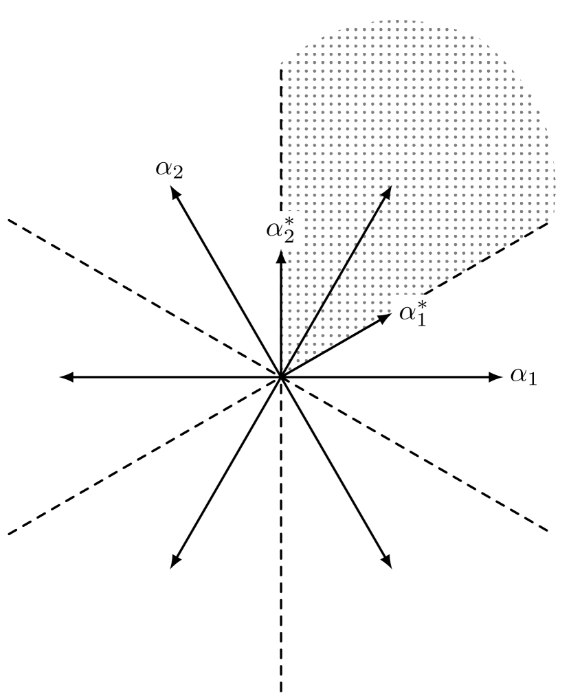
(a) Fundamental Weyl chamber of $\mathrm{SU}(3)$.

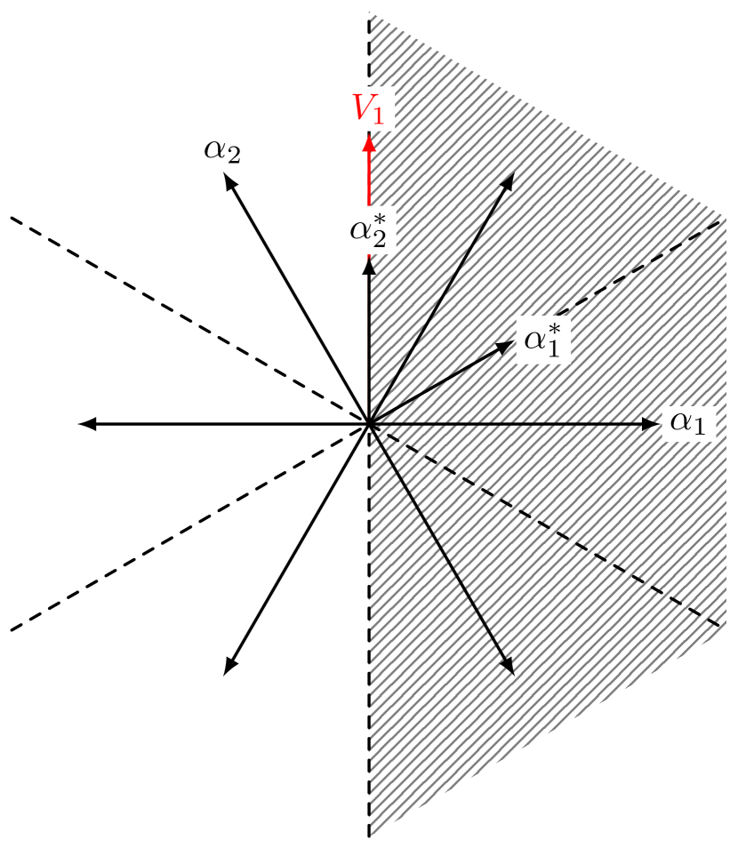
(b) Domain for $W_{1}$ after a specific $V_{1}$ was chosen.

Figure 2: These figures illustrate the algorithm to divide out the Weyl symmetry from the search process, exemplified at the root space of $\mathrm{SU}(3)$. In figure 2(a) the first vector $V_{1}$ can be restricted to lie in the fundamental Weyl chamber of $\mathrm{SU}(3)$ (shaded area) defined by the Weyl reflections $w_{1}$ and $w_{2}$. Thus, $d_{1\,I}\in\mathbbm{N}_{0}$ for $I=1,2$. In figure 2(b) we have chosen a specific vector $V_{1}$ along the direction of $\alpha_{2}^{*}$ as an example. Consequently, the vector $V_{1}$ is invariant under the Weyl reflection $w_{1}$, i.e. $w_{1}(V_{1})=V_{1}$, which corresponds to a vanishing Dynkin label $V_{1}\cdot\alpha_{1}=0$. Hence, this choice for $V_{1}$ has not broken the whole Weyl symmetry and we can use the unbroken Weyl reflection $w_{1}$ to restrict the search space for $W_{1}$ to the enlarged Weyl chamber (shaded area) which is defined by $W_{1}\cdot\alpha_{1}\geq 0$. Hence, the coefficients of $W_{1}$ can be constrained as $d_{3\,1}\in\mathbbm{N}_{0}$ and $d_{3\,2}\in\mathbbm{Z}$. This procedure is continued for the next vectors and takes at each step all previously chosen vectors into account for computing the respective unbroken Weyl symmetry.

To achieve this we expand our vectors not in the basis of the simple roots $\alpha_{I}$ but in the dual basis $\alpha_{I}^{*}$, see eq. (2), where we can apply the constraints on the Dynkin labels directly via the coefficients $d_{k\,I}$ of the gauge embedding matrix. For the first vector, i.e. the shift vector $V_{1}$, we have the full freedom of the Weyl group and can therefore choose this vector directly from the fundamental Weyl chamber

$$V_{1}\cdot\alpha_{I}~{}=~{}\frac{d_{1\,I}}{N_{1}}~{}\geq~{}0\quad\Leftrightarrow\quad d_{1\,I}~{}\in~{}\mathbbm{N}_{0}\;,$$ (9)

for $I=1,\ldots,16$. Thereafter, we have to compute the unbroken Weyl symmetry that can be exploited to restrict the second vector. This unbroken Weyl symmetry is generated by those Weyl reflections that leave $V_{1}$ invariant, i.e. $V_{1}$ has to be a fixed point of a Weyl reflection such that this Weyl reflection remains unbroken. Since we have chosen $V_{1}$ from the fundamental Weyl chamber it can only be a fixed point under a Weyl reflection if $V_{1}$ lies on the boundary of the fundamental Weyl chamber. This boundary is given by the union of the hyperplanes perpendicular to the simple roots, i.e. the hyperplanes at which the Weyl reflections $w_{I}$ act [42]. Consequently, only those Weyl reflections $w_{I}$ which leave all previously chosen vectors $M_{k}$ invariant can still restrict the search space of the shift vector and Wilson lines that have to be chosen next. Therefore, at step $n$ in figure 1 we can constrain the coefficients $d_{n\,I}$ of the vector $M_{n}$ in eq. (2) as

$$d_{n\,I} \in\mathbbm{N}_{0}\quad\text{ if } d_{k\,I}~{}=~{}0\quad\text{for all }k=1,\dots,n-1\;,$$ (10a)

$$d_{n\,I} \in\mathbbm{Z}_{\phantom{0}}\quad\text{ if } d_{k\,I}~{}\neq~{}0\quad\text{for any }k=1,\dots,n-1\;.$$ (10b)

position	frequency	type of model
	of occurrence
1	8 008	gauge group $\mathrm{U}(1)^{16}$ (with $218$ matter fields)
⋮	⋮
19	1 915	first non-Abelian gauge group (gauge group $\mathrm{SU}(2)\times\mathrm{U}(1)^{15}$)
⋮	⋮
3 700	114	first gauge group $\mathrm{SU}(3)\times\mathrm{SU}(2)$
⋮	⋮
119 911	10	first MSSM-like model with 1 generation plus vector-like exotics
⋮	⋮
1 097 248	2	first MSSM-like model with 2 generations plus vector-like exotics
⋮	⋮
3 560 178	1	first MSSM-like model with 3 generations plus vector-like exotics

Table 2: $10^{7}$ random models from the $\mathbbm{Z}_{6}$-II orbifold geometry, ordered by their frequency of occurrence. We list only the first appearances of some special models according to the properties given in the last column. Note that the last position in this list would be $3\,690\,513$ as this is the number of inequivalent models in this dataset.

3 Phenomenological constraints

Obviously, we have to neglect any orbifold model specified by a gauge embedding matrix $M$ that does not obey the stringy consistency conditions on $M$: the geometrical constraints and the modular invariance conditions. Similarly, we can add phenomenologically inspired constraints on $M$: Any orbifold model whose four-dimensional gauge symmetry $G_{4D}(M)$ does not contain the one of the SM does not provide a valid model to describe nature. Importantly, if we search in the heterotic orbifold landscape taking only the stringy consistency condition into account, these phenomenologically uninteresting models build by far the main part of the heterotic orbifold landscape. We have verified this by constructing $10^{7}$ random models in the $\mathbbm{Z}_{6}$-II orbifold geometry that satisfy all stringy consistency conditions using the fundamental Weyl chamber search algorithm. These $10^{7}$ models give rise to approximately $3.5\cdot 10^{6}$ inequivalent massless spectra. Then, the inequivalent spectra are sorted according to their frequency of occurrence inside the full list of $10^{7}$ random models. The result is shown in figure 3 and details on some of the inequivalent spectra are highlighted in table 2. Consequently, from a phenomenological point of view the most uninteresting models turn out to have the highest repetition values, and the most interesting models are the rarest. As a remark, we cannot explain this imbalance, for example, by $\mathrm{E}_{8}\times\mathrm{E}_{8}$ lattice translations and Weyl reflections. Since the models are compared on the level of their massless spectra, it is likely that a lot of these models actually differ by some additional model parameters, for instance by their Yukawa couplings. Nevertheless, we want to avoid these uninteresting models in our search for MSSM-like orbifold models. Therefore, we will describe in the upcoming sections how we can constrain our search to those areas of the heterotic orbifold landscape that can potentially host the SM.

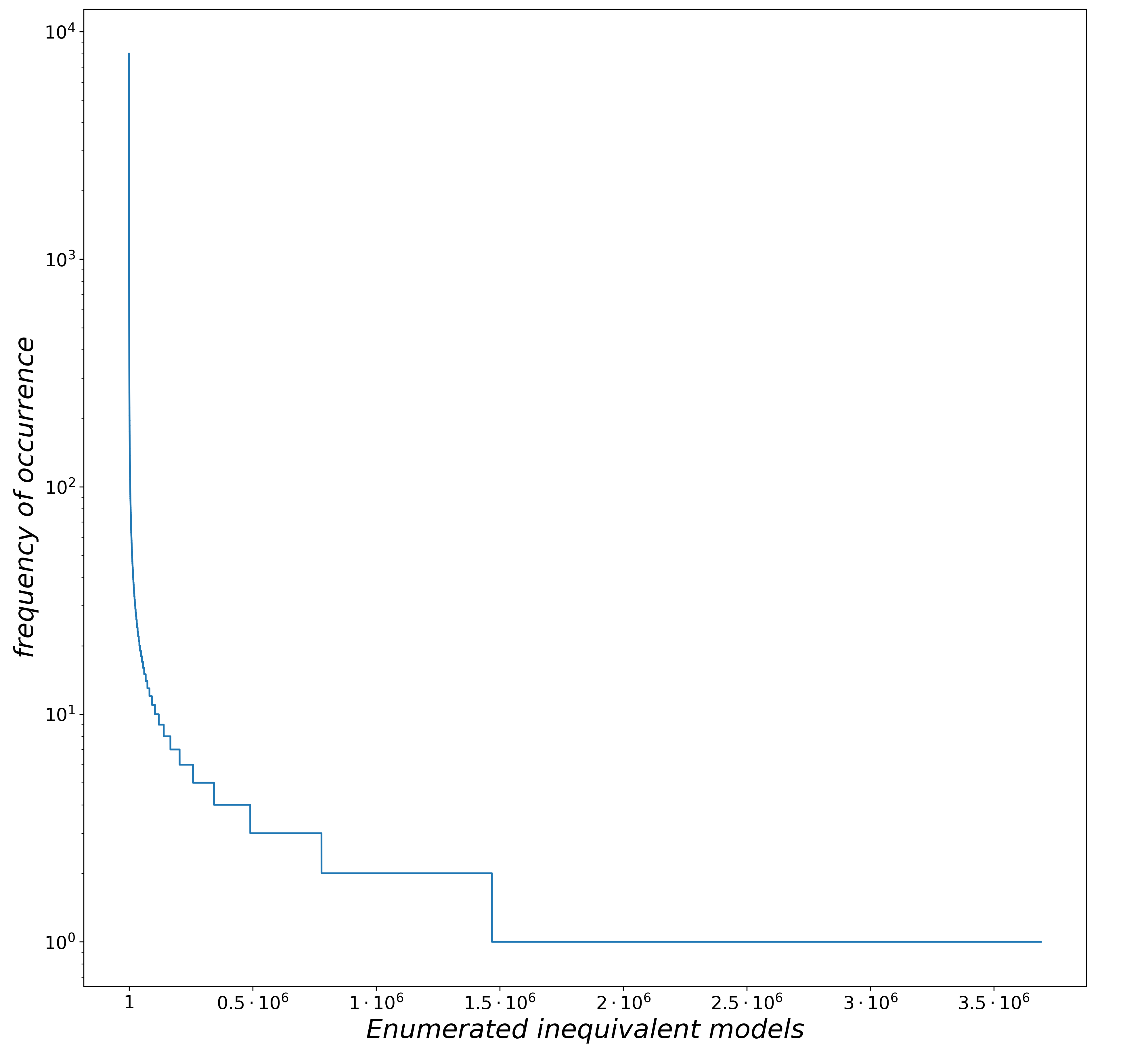
Figure 3: Logarithmic plot of the frequency of occurrence of inequivalent $\mathbbm{Z}_{6}$-II orbifold models. On the horizontal axis, the inequivalent models are enumerated from $1$ to $3\,690\,513$, while on the vertical axis we see the corresponding frequency of occurrence, i.e. model # 1 has a frequency of $8\,008$, see also table 2 for more details on some of these models.

3.1 The pseudo-GUT constraint $G_{n}(M)\geq G_{\mathrm{SM}}^{\prime}$

We want to avoid to produce phenomenologically uninteresting models that have a gauge group smaller than the SM gauge group factors $G_{\mathrm{SM}}^{\prime}=\mathrm{SU}(3)\times\mathrm{SU}(2)$. Hence, we can check how far the gauge group $G_{n}(M)$ is already broken at each step $n=1,\ldots,8$ in the algorithm illustrated in figure 1. Since additional shift vectors or Wilson lines can only break the gauge group further, i.e. $G_{n+1}(M)\subseteq G_{n}(M)$, the SM gauge group provides us with a lower bound on the breaking pattern at each step $n$. A fast way to check the size of the remaining gauge group $G_{n}(M)$ is to compute the number of unbroken roots $N_{\mathrm{sr}}$ after the first $n$ vectors $M_{k}$, for $k=1,\ldots,n$, have been chosen to specify a consistent gauge embedding matrix $M$,

$$N_{\mathrm{sr}}^{(\alpha)}(M)~{}=~{}\sum_{p\,\in\,\Phi_{\mathrm{E}_{8}}}\left(\prod\limits_{k\,=\,1}^{n}\delta\left(p\cdot M_{k}^{(\alpha)}\right)\right)\;,$$ (11)

for $\alpha=1,2$ corresponding to both $\mathrm{E}_{8}$ factors and $\Phi_{\mathrm{E}_{8}}$ is defined as the root system of $\mathrm{E}_{8}$ with 240 roots $p$. Furthermore, $\delta(x)=1,0$ depending on whether $x$ is integer or not, respectively. In the case of the SM we have six unbroken roots for $\mathrm{SU}(3)$ and two unbroken roots for the $\mathrm{SU}(2)$ factor, i.e. $N_{\mathrm{sr}}(\mathrm{SM})=8$. This is our lower bound at each step $n$ in the production of our model $M$ for the first $\mathrm{E}_{8}$ factor, i.e.

$$N_{\mathrm{sr}}^{(1)}(M)~{}\geq~{}8\quad\mathrm{at\ each\ step}\ n\;.$$ (12)

On the other hand, the second $\mathrm{E}_{8}$ factor is free to produce any additional hidden gauge groups. Note that $\mathrm{SU}(2)\times\mathrm{SU}(2)\times\mathrm{SU}(2)\times\mathrm{SU}(2)$ could fulfill the constraint (12) but is already broken too far. Due to this we demand in addition that one gauge factor of $G_{n}(M)$ has a root system that allows for $\mathrm{SU}(3)$, i.e. with six or more unbroken roots. If a newly chosen vector $M_{k}$ results in a gauge group breaking below these lower bounds, we neglect this vector and choose the same vector again, until it fulfills this constraint. In the following we call this constraint the pseudo-GUT constraint.

3.2 The Standard Model gauge group constraint: $\mathrm{SU}(3)\times\mathrm{SU}(2)\subseteq G_{4D}(M)$

The pseudo-GUT constraint is a necessary condition for a model to contain the non-Abelian gauge group factors $G_{\mathrm{SM}}^{\prime}=\mathrm{SU}(3)\times\mathrm{SU}(2)$ of the SM at each step of the construction of the gauge embedding matrix $M$. However, our search focuses on MSSM-like models with $\mathrm{SU}(3)_{\mathrm{C}}\times\mathrm{SU}(2)_{\mathrm{L}}\times\mathrm{U}(1)_{Y}$ gauge symmetry in 4D and not on grand unified models like Pati-Salam or $\mathrm{SU}(5)$. Hence, after we have chosen the last vector $M_{k}$ of our orbifold model (taking the geometrical constraints into account), we can check that the model $M$ has a 4D gauge symmetry

$$G_{4D}(M)~{}=~{}\mathrm{SU}(3)\times\mathrm{SU}(2)\times G_{\mathrm{hidden}}\;.$$ (13)

We denote this constraint by $\mathrm{SU}(3)\times\mathrm{SU}(2)\subseteq G_{4D}(M)$.

Due to the geometrical constraints, we first have to identify the last shift vector or Wilson line that can be chosen independently, i.e. which is not of order one and not equal to a previous vector. For example, for the $\mathbbm{Z}_{6}$-II orbifold geometry this results in the Wilson line $W_{6}$, as can be seen in table 2. However, note that for some other orbifold geometries like $\mathbbm{Z}_{3}\!\times\!\mathbbm{Z}_{6}$ $(2,2)$ all Wilson lines are fixed by the geometry, $W_{i}=(0^{16})$ for $i=1,\ldots,6$, and the second shift vector $V_{2}$ has to enable the $G_{4D}(M)$ constraint. The constraint is checked by computing the unbroken roots from the first $\mathrm{E}_{8}$ factor and the sizes of their orthogonal root systems. This means that in order to contain $\mathrm{SU}(3)\times\mathrm{SU}(2)$ at least two root systems, one of size six and another of size two, have to be present, where we allow for additional gauge group factors, also from the first $\mathrm{E}_{8}$ factor.

We implement the phenomenological constraints from section 3.1 and section 3.2 into our search algorithm and apply it to the test case of $\mathbbm{Z}_{6}$-II orbifold models. It turns out that the probability of finding an MSSM-like model increases by a factor $10$ from $\tfrac{1}{10\,000\,000}=10^{-7}$ in the case without the phenomenological constraints to $\tfrac{3}{2\,665\,463}\approx 10^{-6}$ in the case where the phenomenological constraints are applied. In addition, we use physical intuition that MSSM-like models are often related to a vanishing Wilson line [20] and perform a second search where we set $W_{5}=(0^{16})$ by hand. The results are summarized in table 3 (where the corresponding dataset is called phenomenology).

	dataset	condition	# models	# MSSM-like	# inequiv. MSSM-like
traditional	fundamental Weyl		$10\,000\,000$	1	1
	chamber
	phenomenology		$2\,665\,463$	3	3	130
		$W_{5}=(0^{16})$	$2\,551\,272$	509	129
contrast patterns	hidden $E_{8}$		$2\,543\,415$	12	11	136	415	468
		$W_{5}=(0^{16})$	$2\,609\,872$	863	135
	dynamic hidden $E_{8}$		$1\,876\,273$	3 299	245	395
		$W_{5}=(0^{16})$	$1\,231\,608$	8 455	321
		$W_{3}=(0^{16})$	$378\,604$	7	2
	U-sector		$4\,793\,146$	4 953	357	459
		$W_{5}=(0^{16})$	$3\,046\,262$	17 406	358

Table 3: Datasets created in the $\mathbbm{Z}_{6}$-II orbifold landscape. Each dataset incorporates all of the constraints, indicated by the names in the first column, of the datasets above. The fundamental Weyl chamber dataset utilizes the Weyl symmetry, see section 2.3, while the phenomenology dataset makes additionally use of the constraints developed in section 3. In the next rows, we apply our contrast patterns: first, we demand $N_{\mathrm{sr}}^{(2)}\geq 6$ from section 4.2.1 and obtain the hidden $E_{8}$ dataset. Note that in the dynamic search we modify this constraint as explained in section 4.2.2 to $N_{\mathrm{sr}}^{(2)}\geq X$ for $X\in\{8,10,12,\ldots,86\}$ and obtain the dynamic hidden $E_{8}$ dataset. Here, the case $X=6$ was disregarded since it was already sampled in the hidden $E_{8}$ dataset. Finally, the U-sector dataset was created using the U-sector contrast pattern from section 4.2.3 in addition. Note that we also made use of the additional conditions $W_{5}=(0^{16})$ or $W_{3}=W_{4}=(0^{16})$, where $W_{5}=(0^{16})$ is known to be beneficial for finding MSSM-like models, see ref. [20].

4 Contrast patterns for $\mathbbm{Z}_{6}$-II orbifolds

In the previous section, we discussed phenomenological constraints that can be checked easily during the search for MSSM-like orbifold models. Importantly, these conditions are absolutely necessary for a model to be MSSM-like (but not sufficient). Now, we want to extend this procedure to include additional constraints (so-called contrast patterns) for MSSM-like models by exploiting techniques from data mining. These new constraints will be determined by a statistical approach. Hence, demanding them can potentially rule out a few MSSM-like models. In other words, the new constraints are not necessarily satisfied for all MSSM-like models but they significantly enhance the probability for a given model to be MSSM-like. In this way, we will constrain the heterotic orbifold landscape further to the areas of MSSM-like models. Some of these areas are hardly accessible by the conventional search algorithm but easy to access due to the significantly enhanced probability given the additional constraints from the contrast patterns.

A contrast pattern $c$ can be defined as a pattern whose supports differ significantly among the datasets under contrast [43]. Here, the support is defined as

$$\mathrm{supp}(c,D)~{}=~{}\dfrac{|\{M\in D\ |\ M~{}\mathrm{satisfies}~{}c\}|}{|D|}\;,$$ (14)

where $D$ is a set of data points, i.e. orbifold models, and $c$ is a set of certain constraints that have to be fulfilled. In our case, we have two datasets that are under contrast: $D_{\text{MSSM-like}}$ and $D_{\text{\cancel{MSSM}-like}}$, which is the set of MSSM-like models and the complementary set, respectively. In other words, we are searching for constraints $c$ that are satisfied for nearly all MSSM-like models while they are violated by a huge fraction of MSSM-like models. In the ideal case, we can identify contrast patterns $c$ with $\mathrm{supp}(c,D_{\text{MSSM-like}})=1$ and $\mathrm{supp}(c,D_{\text{\cancel{MSSM}-like}})=0$. This can be formalized by defining the growth rate

$$\mathrm{gr}(c,D_{\text{MSSM-like}},D_{\text{\cancel{MSSM}-like}})~{}=~{}\dfrac{\mathrm{supp}(c,D_{\text{MSSM-like}})}{\mathrm{supp}(c,D_{\text{\cancel{MSSM}-like}})}\;,$$ (15)

which has to be maximized. In the following, we will often just write $\mathrm{gr}(c)$ if the datasets $D_{\text{MSSM-like}}$ and $D_{\text{\cancel{MSSM}-like}}$ are clear from the context.

To understand the growth rate better and get some intuition for its value, we rewrite it in terms of the probability $\hat{p}$. Here, the hat indicates that we estimate the probability by the sample proportion $\hat{p}(Y)=\nicefrac{{N_{Y}}}{{N}}$, where $Y\in\{$MSSM-like, MSSM-like$\}$ and the total sample size is given by $N=N_{\text{MSSM-like}}+N_{\text{\cancel{MSSM}-like}}$. Then, one finds

$$\mathrm{gr(c)}=\dfrac{\hat{p}^{c}(\text{MSSM-like})}{\hat{p}(\text{MSSM-like})}\dfrac{\hat{p}(\text{\cancel{MSSM}-like})}{\hat{p}^{c}(\text{\cancel{MSSM}-like})}\;,$$ (16)

where $\hat{p}^{c}(Y)=\nicefrac{{N^{c}_{Y}}}{{N^{c}}}$ with $N^{c}_{Y}=|\{M\in D_{Y}\ |\ M~{}\mathrm{satisfies}~{}c\}|$ is the probability of a model being $Y=$ MSSM-like or $Y=$ MSSM-like given the constraints $c$ and $\hat{p}(Y)$ is the corresponding probability without imposing the constraints $c$. Then, one can solve eq. (16) for $\hat{p}^{c}(\text{MSSM-like})$ as a function of $\hat{p}(\text{MSSM-like})$ as follows

$$\hat{p}^{c}(\text{MSSM-like})~{}=~{}\dfrac{\mathrm{gr(c)}\,\hat{p}(\text{MSSM-like})}{1+(\mathrm{gr(c)}-1)\hat{p}(\text{MSSM-like})}\;.$$ (17)

Here, one can observe several cases:

$$\hat{p}(\text{MSSM-like})~{}\ll~{}1\ :\ \hat{p}^{c}(\text{MSSM-like})~{}=~{}\text{gr(c)}\hat{p}(\text{MSSM-like})+\mathcal{O}\!\left(\hat{p}(\text{MSSM-like})^{2}\right)\;,$$ (18a)

$$\text{gr(c)}~{}=~{}1\ :\ \hat{p}^{c}(\text{MSSM-like})~{}=~{}\hat{p}(\text{MSSM-like})\;,$$ (18b)

$$\mathrm{gr(c)}~{}=~{}0\ :\ \hat{p}^{c}(\text{MSSM-like})~{}=~{}0\;,$$ (18c)

$$\mathrm{gr(c)}~{}\rightarrow~{}\infty\ :\ \hat{p}^{c}(\text{MSSM-like})~{}\rightarrow~{}1\;,$$ (18d)

where the Taylor expansion in eq. (18a) converges for $\hat{p}(\text{MSSM-like})<\tfrac{1}{|\mathrm{gr}(c)-1|}$. Now, eq. (18a) can be interpreted easily: For $\mathrm{gr}(c)<1$ we have a negative effect on our favored class of MSSM-like models. For $\mathrm{gr}(c)=1$ the effects on both classes cancel each other and for $\mathrm{gr}(c)>1$ we have a positive effect, i.e. a higher probability to find MSSM-like models in the subspace defined by the contrast patterns $c$.

However, before we can start to search for contrast patterns $c$, we have to define some (physical) quantities that possibly can lead to such patterns. This is known as feature engineering as explained in the next section.

4.1 Feature engineering

In this section, we will define (physical) quantities for a given orbifold model $M$. In the context of data mining, we will call such quantities features and their construction is called feature engineering. In general terms, feature engineering denotes the process of computing useful quantities from the raw data. For example, neural networks generate features in each hidden layer on their own during training. However, this is one of the biggest open problems of neural networks: it is in general very difficult to extract any meaning of the features that a neural network has learned on its own – these features hardly yield any knowledge gain. Alternatively, in this paper we will use physical intuition and knowledge of the system to create features. Then, after visualizing some of these features, we can use machine learning techniques (i.e. a decision tree) to quantify if our educated guess for a certain feature, or combinations of multiple features, leads to a correlation between these features and the property of $M$ being MSSM-like or not. If such a correlation exists (i.e. if $\mathrm{gr}(c)>1$), we have identified a promising contrast pattern $c$. Moreover, if we can check this pattern $c$ easily in the search algorithm displayed in figure 1, we can utilize it to reduce the search space in the heterotic orbifold landscape to areas where MSSM-like orbifold models accumulate. The advantage of this approach is obvious: by construction we have a straightforward physical interpretation of our features.

However, in general it is very difficult to identify useful features. In our case, we have tried many concepts, for instance, local GUTs, the breaking patterns of each shift vector and each Wilson line, the breaking patterns of certain combinations thereof, the number of non-Abelian gauge group factors in 4D, and many more. We know from section 2 that the 4D gauge group has a great impact and it can be checked easily at every step of the production of a model. Therefore, there is hope that additional features can be found from the 4D gauge group. When attempting to identify a promising feature, data visualization can be very useful: In figure 4, we plot the number of unbroken roots $N_{\mathrm{sr}}^{(\alpha)}$ from each $\mathrm{E}_{8}$ factor in a scatter plot against each other using the phenomenology dataset created in section 3. In addition, the respective histograms for the number of orbifold models with a certain number of unbroken roots are displayed in figure 4 for each axis (i.e. for each $\mathrm{E}_{8}$ factor).

Figure 4: Jointplot (see ref. [44]) of $N_{\mathrm{sr}}^{(1)}$ and $N_{\mathrm{sr}}^{(2)}$ for the complete phenomenology dataset of $\mathbbm{Z}_{6}$-II orbifold models, see table 3. Due to the constraint $\mathrm{SU}(3)\times\mathrm{SU}(2)\subseteq G_{4D}(M)$ from section 3.2 we have a bound $N_{\mathrm{sr}}^{(1)}\geq 8$ in this dataset. The central part shows a scatter plot, where MSSM-like and MSSM-like orbifold models are marked by blue circles and red boxes, respectively. Above and on the right hand side of the scatter plot we give the histogram on the number of models for given values of $N_{\mathrm{sr}}^{(1)}$ and $N_{\mathrm{sr}}^{(2)}$, respectively. Note that the number of MSSM-like models is negligible compared to the MSSM-like models in this dataset. Hence, the histograms visualize the frequency of occurrence for MSSM-like models only.

To see if the feature $N_{\mathrm{sr}}^{(\alpha)}$ has the potential to be useful as a contrast pattern, we have to pay attention to two aspects of this plot. First, we have to identify areas in this plot where no MSSM-like orbifold model is present. Second, it is important that such an area is not only qualitatively separated from MSSM-like orbifold models but also quantitatively interesting, i.e. highly populated with MSSM-like orbifold models. This aspect can be read off from the respective histogram in figure 4. By doing so, we identify the area $N_{\mathrm{sr}}^{(2)}<6$ that does not contain any MSSM-like $\mathbbm{Z}_{6}$-II orbifold model but is fairly high populated with MSSM-like models in our phenomenology dataset. Hence, the condition $N_{\mathrm{sr}}^{(2)}<6$ is our first promising candidate for a contrast pattern and we expect to get a strong reduction of the $\mathbbm{Z}_{6}$-II orbifold landscape by excluding this area form the search. In contrast, an example of an area that consists of MSSM-like $\mathbbm{Z}_{6}$-II models only but is irrelevant due to the small number of models is given by $N_{\mathrm{sr}}^{(2)}>42$ or $N_{\mathrm{sr}}^{(1)}>20$: the respective histograms (in figure 4, the vertical histogram on the right-hand side for $N_{\mathrm{sr}}^{(2)}>42$ and the horizontal histogram above the scatter plot for $N_{\mathrm{sr}}^{(1)}>20$) show that the number of $\mathbbm{Z}_{6}$-II orbifold models in these regions is very small.

In addition to the above features, we will also use the numbers of orbifold-invariant bulk matter fields as additional features. They are computed similar to the number of unbroken roots of the gauge group in eq. (11), with the difference of an additional displacement from the geometrical twist vector $v$, i.e. at each step $n$ of our search algorithm displayed in figure 1 we compute

$$N_{\mathrm{U}_{a}}^{(\alpha)}(M)~{}=~{}\sum_{p\,\in\,\Phi_{\mathrm{E}_{8}}}\prod\limits_{k\,=\,1}^{n}\delta\left(p\cdot M_{k}^{(\alpha)}-\Theta(2-k)\,q_{(a)}\cdot v_{(k)}\right)\;,$$ (19)

for $\alpha=1,2$ and $a=1,2,3$. Note that the term $q_{(a)}\cdot v_{(k)}$ in eq. (19) is turned off for the Wilson lines $M_{k}^{(\alpha)}$, $k=3,\ldots,8$, using

$$\Theta(x)~{}=~{}\begin{cases}0\quad\mathrm{if}&x<0\\ 1\quad\mathrm{if}&x\geq 0\;.\end{cases}$$ (20)

Furthermore, the vectors $q_{(1)}=(0,-1,0,0)$, $q_{(2)}=(0,0,-1,0)$ and $q_{(3)}=(0,0,0,-1)$ give rise to the three untwisted sectors $\mathrm{U}_{a}$, $a=1,2,3$, and correspond to the three directions of the internal vector-boson index of the ten-dimensional $\mathrm{E}_{8}\times\mathrm{E}_{8}$ gauge bosons, respectively. Finally, the twist vectors in eq. (19) are given by $v_{(1)}=(0,\tfrac{1}{6},\tfrac{1}{3},-\tfrac{1}{2})$ and $v_{(2)}=(0^{4})$ is not present for the $\mathbbm{Z}_{6}$-II orbifold geometry. Due to the $\delta$-condition in eq. (19) all features $N_{\mathrm{U}_{a}}^{(\alpha)}(M)$ and $N_{\mathrm{sr}}^{(\alpha)}(M)$ are independent.

	first $\mathrm{E}_{8}$				hidden $\mathrm{E}_{8}$
feature	$N_{\mathrm{sr}}^{(1)}$	$N_{\mathrm{U}_{1}}^{(1)}$	$N_{\mathrm{U}_{2}}^{(1)}$	$N_{\mathrm{U}_{3}}^{(1)}$	$N_{\mathrm{sr}}^{(2)}$	$N_{\mathrm{U}_{1}}^{(2)}$	$N_{\mathrm{U}_{2}}^{(2)}$	$N_{\mathrm{U}_{3}}^{(2)}$

Table 4: Overview table of the features that we use for contrast mining. Each feature is evaluated for all orbifold models $M$ of the dataset under investigation.

4.2 Decision tree and false negatives

In this section, we will use a decision tree [45] in order to identify those features from table 4 that correlate with the property of a model being MSSM-like or not. If such a correlation exists, the corresponding feature can be used as contrast pattern in our search algorithm for MSSM-like orbifold models. A decision tree belongs to the class of supervised machine learning and can be used for the purpose of classification or regression. In our case, we want to classify whether a given orbifold model is MSSM-like or not using simple true-or-false decisions on the features listed in table 4. Then, by analyzing the decisions made inside of the decision tree, we can identify those features that lead to successful contrast patterns.

In more detail, our decision tree is a function from some of the features listed in table 4 to the classification value denoted by $Y$, i.e. it is of the form

$$\left(N_{\mathrm{sr}}^{(1)}(M),N_{\mathrm{U}_{1}}^{(1)}(M),N_{\mathrm{U}_{2}}^{(1)}(M),N_{\mathrm{U}_{3}}^{(1)}(M),\ldots,\right)~{}\mapsto~{}Y_{\mathrm{predicted}}(M)\;,$$ (21)

where $Y_{\mathrm{predicted}}(M)\in\{\text{MSSM-like},\text{\cancel{MSSM}-like}\}$, and it can be applied to all orbifold models $M$. Note that we can compute for each orbifold model $M$ both, the features and the correct classification value $Y_{\mathrm{correct}}(M)\in\{\text{MSSM-like},\text{\cancel{MSSM}-like}\}$ using the orbifolder. Yet, the benefit of using a decision tree is given by the possibility to uncover unknown correlations between our features and the property $Y_{\mathrm{correct}}(M)$ of an orbifold model $M$ to be MSSM-like or not. Furthermore, it is by no means guaranteed that a function like eq. (21) exists. We will only know about its existence after we have trained and tested our decision tree.

In a first step, the decision tree has to be trained, i.e. the algorithm tries to learn the function (21). To do so, it needs a training set, i.e. a list of orbifold models, where for each orbifold model $M_{i}$ we have computed the values of our features and the correct classification values $Y_{\mathrm{correct}}(M_{i})$ using the orbifolder. More explicitly, the training set reads

training set $$= \{\{N_{\mathrm{sr}}^{(1)}(M_{1}),N_{\mathrm{U}_{1}}^{(1)}(M_{1}),N_{\mathrm{U}_{2}}^{(1)}(M_{1}),N_{\mathrm{U}_{3}}^{(1)}(M_{1}),\ldots,Y_{\mathrm{correct}}(M_{1})\},$$ (22)

$$\,\,\{N_{\mathrm{sr}}^{(1)}(M_{2}),N_{\mathrm{U}_{1}}^{(1)}(M_{2}),N_{\mathrm{U}_{2}}^{(1)}(M_{2}),N_{\mathrm{U}_{3}}^{(1)}(M_{2}),\ldots,Y_{\mathrm{correct}}(M_{2})\},\ldots\}\;,$$

and during training the decision tree tries to adjust the function eq. (21) such that $Y_{\mathrm{predicted}}(M)=Y_{\mathrm{correct}}(M)$ for all models $M$ from the training set. After training, we can evaluate the trained decision tree (21) on the so-called validation set

validation set $$= \{\{N_{\mathrm{sr}}^{(1)}(P_{1}),N_{\mathrm{U}_{1}}^{(1)}(P_{1}),N_{\mathrm{U}_{2}}^{(1)}(P_{1}),N_{U\mathrm{U}_{3}}^{(1)}(P_{1}),\ldots,Y_{\mathrm{correct}}(P_{1}))\},$$ (23)

$$\,\,\{N_{\mathrm{sr}}^{(1)}(P_{2}),N_{\mathrm{U}_{1}}^{(1)}(P_{2}),N_{\mathrm{U}_{2}}^{(1)}(P_{2}),N_{U\mathrm{U}_{3}}^{(1)}(P_{2}),\ldots,Y_{\mathrm{correct}}(P_{2})\},\ldots\}\;,$$

containing the features of some other orbifold models $P_{i}$. Then, we can compare the results $Y_{\mathrm{predicted}}(P_{i})$ of the decision tree (21) to the correct values $Y_{\mathrm{correct}}(P_{i})$ obtained from the orbifolder. In this way, we can check whether our decision tree was able to identify the function eq. (21) between our features and the property of a model being MSSM-like or not.

In practice, a decision tree will not be trained perfectly. First of all, it is possible that there is no exact functional dependency of the form eq. (21). Furthermore, even in the case when such a functional dependency would exist in principle, the decision tree might be unable to learn it, possibly because the training set was too small or imbalanced. In general, we can distinguish between two types of errors, i.e. cases where $Y_{\mathrm{correct}}(M)\neq Y_{\mathrm{predicted}}(M)$. They are called:

• false positives: $Y_{\mathrm{correct}}(M)=$ MSSM-like but $Y_{\mathrm{predicted}}(M)=$ MSSM-like

• false negatives: $Y_{\mathrm{correct}}(M)=$ MSSM-like but $Y_{\mathrm{predicted}}(M)=$ MSSM-like

Every classification process tries to minimize the number of false predictions. However, at a certain level it always comes to a trade-off between false positives and false negatives and we have to decide whether we want to suppress one of them for the drawback of raising the other one. In our case, a false positive classification by the decision tree is not a big problem since we can simply check each of these orbifold models afterwards explicitly using the orbifolder. However, in the case of a false negative classification the consequences are that we will loose an MSSM-like orbifold model. Since MSSM-like orbifold models are far too valuable to us, we want to minimize the number of false negative cases by all means, while we want to keep the number of false positives as low as possible. Therefore, we introduce a loss matrix $L$, which informs the machine learning algorithm about the different importance of certain models [46]. We choose a loss matrix

$$L=\left(\begin{array}[]{cc}0&10^{6}\\ 1&0\end{array}\right)~{},$$ (26)

where the two rows correspond to the correct value $Y_{\mathrm{correct}}(M)$ being either MSSM-like or not, and the two columns correspond to the predicted values $Y_{\mathrm{predicted}}(M)$ being either MSSM-like or not. Then, $L_{12}$ corresponds to the false negative cases of an MSSM-like orbifold model $M$ that has been classified by the decision tree to be $Y_{\mathrm{predicted}}(M)=$ MSSM-like. As this is very undesirable, the system is punished with a large loss value $L_{12}=10^{6}$. As discussed before, the other possible error of a false positive classification is not so severe. Hence, we set $L_{21}=1$. This will guide the decision tree algorithm towards suppressing the false negative cases such that we do not miss any MSSM-like orbifold models.

For later convenience, we will quantify the quality of the predictions by the recall. It is defined as the number of correct predictions of the MSSM-like class divided by the total number of MSSM-like orbifold models. Hence, if the number of false negatives for all MSSM-like orbifold models $P_{i}$ is zero, the recall is $1.00$ on the validation set and all MSSM-like orbifold models are assigned with the correct value $Y=$ MSSM-like.

In the following, we apply decision trees to our features in order to extract promising contrast patters.

4.2.1 The hidden $E_{8}$ contrast pattern

As a first step, we have to define our datasets. The training and validation set are created by a random split (using a validation size of 33%) of the phenomenology dataset from table 3 (based on the phenomenological constraints from section 3.1 and section 3.2). However, we add a small modification to the dataset to avoid data leakage. Data leakage refers to the mistake to inform the machine learning algorithm about data from the validation set during training. In this case, the machine learning algorithm might overfit on some of the data from the validation set even though the data was divided into training and validation set. As the performance of a machine learning model on the validation set is a measure for its ability to generalize to unseen data, this mistake has to be avoided. In our case this could happen if, for example, there exists an MSSM-like model that completely dominates all MSSM-like models with all of its equivalent copies. Then, this model would appear most likely in both, training and validation set. Hence, the machine learning algorithm would see this model during training. Moreover, the same model would dominate the results on the validation set and pretend that the learned predictions generalize to generic MSSM-like models. Therefore, to avoid data leakage we only use inequivalent MSSM-like models. Nevertheless, for the MSSM-like models we keep the equivalent models, since the frequency of occurrence gives us a notion of the size of the area that a certain split in the decision tree excludes. In more detail, we have to perform our search for MSSM-like orbifold models in the space $\mathbbm{Z}^{128}$ of gauge embedding matrices $\{M_{i}\}$, see eq. (2), even though we are interested in the space of physically inequivalent models $\{\mathrm{model}(M_{j})\}$, or more precisely, in the space of inequivalent massless particle spectra $\{\mathrm{spectrum}(M_{k})\}$. Now, we defined features that directly depend on $\mathrm{spectrum}(M)$, not on $d\in\mathbbm{Z}^{128}$ and our decision tree performs its splits based on these features. Consequently, a certain split in the decision tree will exclude all points $d\in\mathbbm{Z}^{128}$ that give rise to the same excluded features. In this way, a small restriction in feature space gives rise to a huge effect in the space $\mathbbm{Z}^{128}$ of gauge embedding matrices. Moreover, by not restricting the feature space too much, we leave enough room to discover new MSSM-like models, also in unexpected areas of the landscape. In contrast, if we had used only inequivalent MSSM-like models for the training of our decision tree, the decision tree would not care to exclude a single model even though it might actually correspond to a huge area in $\mathbbm{Z}^{128}$. At the end, we want to enhance the search algorithm. Hence, it is better to exclude a few models with extraordinary high frequency of occurrence than multiple models with very low one.

Figure 5: Decision tree on the phenomenology dataset from table 3, evaluated on the training set. We can extract the contrast pattern $N_{\mathrm{sr}}^{(2)}\leq 5$ for MSSM-like models from this tree, which we reformulate into a positive condition $N_{\mathrm{sr}}^{(2)}\geq 6$ for MSSM-like models. Let us explain the details at the example of the uppermost node. This node contains: (i) the condition $G^{\prime}_{SM}$ in both $E_{8}$? that has to be evaluated, (ii) samples=3 494 956 gives the total number of models in this node, (iii) value = $[89,3\,494\,867]$ gives the number of MSSM-like and MSSM-like models in this node, respectively, and, finally, (iv) class = MSSM-like is the prediction for all models in this intermediate node. The final prediction for the models is given by the leaf nodes.

Now, we train the decision tree on the training set. Here, we tune the hyperparameters such that we get a recall value for MSSM-like models of $1.00$ on the validation set. This is due to the fact that we want to find contrast patterns that are satisfied by all MSSM-like models contained in the validation set. During training, the decision tree identifies areas in feature space and assigns the two classes $\{\text{MSSM-like},\text{\cancel{MSSM}-like}\}$ to them, using the data from the training set. However, we want the decision tree to assign the class MSSM-like only to those areas that are also highly populated with MSSM-like models. In this way, we can be sure that the probability for an MSSM-like model is extremely small in these areas of MSSM-like models. This can be achieved using a technique called pruning. Consequently, the complexity of the decision tree is reduced to a minimum and we keep the possibility to find MSSM-like models in rather unexpected areas of the landscape.

The resulting decision tree is displayed in figure 5. We see that the intuition given by the scatter plot in figure 4 manifests in a lower bound on the number of unbroken roots from the hidden $\mathrm{E}_{8}$ factor: From the second node in the second line of the decision tree we can extract the condition

$$c_{\text{hidden $\mathrm{E}_{8}$}}~{}=~{}\Big{\{}N_{\mathrm{sr}}^{(2)}(M)~{}\geq~{}6\Big{\}}\;,$$ (27)

for a model $M$ to have a high probability to be MSSM-like. We call this condition the hidden $E_{8}$ contrast pattern. In principle, our decision tree contains additional splits. However, we want to stay conservative with our search and avoid too enthusiastic splits. Hence, we stay with the first and most important split for now. Based on the training set form our phenomenology dataset we can estimate the growth rate of the hidden $E_{8}$ contrast pattern to be

$$\mathrm{gr}\left(c_{\text{hidden $\mathrm{E}_{8}$}},D_{\text{MSSM-like}},D_{\text{\cancel{MSSM}-like}}\right)~{}=~{}\dfrac{1}{\tfrac{896\,169+551\,319}{3\,494\,867}}~{}\approx~{}2.4~{}>~{}1\;,$$ (28)

using eq. (15) with $\mathrm{supp}(c_{\text{hidden $\mathrm{E}_{8}$}},D_{\text{MSSM-like}})=1$ for our phenomenology dataset and the numbers for $\mathrm{supp}(c_{\text{hidden $\mathrm{E}_{8}$}},D_{\text{\cancel{MSSM}-like}})$ can be read off from figure 5. In other words, we can modify our search algorithm such that we would have avoided $2\,047\,379$ MSSM-like models in the training set. Hence, the contrast pattern (27) allows us to exclude a huge area in the $\mathbbm{Z}_{6}$-II orbifold landscape which statistically does not lead to MSSM-like models. Instead, we can invest the gained computing time to search in areas where the probability of a model to be MSSM-like is significantly increased.

We implement the hidden $E_{8}$ contrast pattern into our search algorithm displayed in figure 1 and perform an intensive search using in addition different constraints on the Wilson lines: First, we allow all Wilson lines to be non-trivial and then, motivated by ref. [20], we turn off $W_{5}$ by hand. The resulting dataset is called hidden $E_{8}$ and summarized in table 3. One observes an increase of the probability to find an MSSM-like model from

$$\hat{p}^{\text{phenomenology}}(\text{MSSM-like}) = \frac{512}{5\,216\,735}~{}\approx~{}10^{-4}\quad\mathrm{to}$$ (29a)

$$\hat{p}^{\text{hidden $\mathrm{E}_{8}$}}(\text{MSSM-like}) = \frac{875}{5\,153\,287}~{}\approx~{}2\cdot 10^{-4}\;,$$ (29b)

which is consistent with the estimated growth rate in eq. (28). However, these are the probabilities to find any MSSM-like model and it does not need to be inequivalent to the already known ones. Unfortunately, the total number of inequivalent MSSM-like models did not satisfy our expectations: it increased from 130 inequivalent MSSM-like models in the phenomenology dataset to 136 in the hidden $E_{8}$ dataset. In the next section, we will investigate the reasons for this and present a solution that will lead to many new inequivalent MSSM-like models.

4.2.2 The dynamic hidden $E_{8}$ contrast pattern

Next, we analyze the effect of the hidden $E_{8}$ contrast pattern in more detail in order to identify a way to improve this constraint further. To do so, we take the (equivalent) MSSM-like $\mathbbm{Z}_{6}$-II models from the hidden $E_{8}$ dataset and visualize how many MSSM-like models $M$ appear for various values of $N_{\mathrm{sr}}^{(2)}(M)$, see figure 6.

Figure 6: Bar chart of MSSM-like $\mathbbm{Z}_{6}$-II models $M$ found using the hidden $E_{8}$ contrast pattern $N_{\mathrm{sr}}^{(2)}(M)\geq 6$. On the horizontal axis we give $N^{(2)}_{\mathrm{sr}}(M)$ corresponding to the number of unbroken roots from the hidden $\mathrm{E}_{8}$. The vertical axis gives the corresponding frequency of occurrence. Each bar stands for an inequivalent MSSM-like model $M$. The number of copies of each model is shown by the height of the bar. As an example, take $N^{(2)}_{\mathrm{sr}}(M)=10$, i.e. the green bars: There are three inequivalent MSSM-like models, each represented by one bar. These inequivalent models have 6, 6 and 7 copies in the whole dataset, respectively. Note that in this chart only those MSSM-like models appear that have $G_{SM}^{\prime}$ only in one $\mathrm{E}_{8}$, since the notion of hidden $\mathrm{E}_{8}$ is ambiguous otherwise.

From this chart we see that the models with small numbers of unbroken roots $N^{(2)}_{\mathrm{sr}}(M)\in\{6,\ldots,14\}$ are heavily oversampled in the hidden $E_{8}$ dataset, while it seems to be very difficult to construct models with $N^{(2)}_{\mathrm{sr}}(M)\geq 30$. Moreover, note that especially for $N^{(2)}_{\mathrm{sr}}(M)=22$ the bar chart shows a lot of different bars, i.e. there are many inequivalent MSSM-like models with $N^{(2)}_{\mathrm{sr}}(M)=22$. This suggests that the diversity of inequivalent MSSM-like models may lie in some areas of the $\mathbbm{Z}_{6}$-II orbifold landscape where models have larger hidden sector gauge groups. Furthermore, we investigate the change of the growth rate for higher threshold values $X$ of our contrast pattern $N^{(2)}_{\mathrm{sr}}(M)\geq X$ and obtain table 5. Therefore, it seems very promising to change the threshold value $X=6$ of the contrast pattern $N^{(2)}_{\mathrm{sr}}(M)\geq X$ into a dynamic variable $X$. We call this new constraint dynamic hidden $E_{8}$. By applying this dynamic contrast pattern, we hope that the sampling among the various sizes of the hidden sector gets more balanced. Furthermore, we expect a boost in the number of MSSM-like models due to the increasing growth rate for higher values of $N^{(2)}_{\mathrm{sr}}(M)$.

$X$	6	8	10	12	…	20	22	…	30	32	…	40	42
$\mathrm{gr}(N^{(2)}_{\mathrm{sr}}(M)\geq X)$	1	5	6	6	…	12	26	…	48	75	…	73	82

Table 5: Change of the growth rate for higher threshold values $X$ of our contrast pattern $N^{(2)}_{\mathrm{sr}}(M)\geq X$, where the reference point is $\mathrm{gr}(N^{(2)}_{\mathrm{sr}}(M)\geq 6)=1$, since this analysis is done in the hidden $E_{8}$ dataset.

We perform an intensive search based on the dynamic hidden $E_{8}$ contrast pattern for various values of the threshold $X$ and different constraints on the Wilson lines: First, we allow all Wilson lines to be non-trivial, then we turn off either $W_{3}=W_{4}$ or $W_{5}$. As a result, we obtain a new dataset (which we also call dynamic hidden $E_{8}$), see table 3. Compared to the hidden $E_{8}$ dataset with 136 inequivalent MSSM-like $\mathbbm{Z}_{6}$-II models we now have in total 415 MSSM-like models. This is already more than in any existing $\mathbbm{Z}_{6}$-II search [19, 20, 17, 18]. Hence, we were able to significantly improve the search for inequivalent MSSM-like models in the $\mathbbm{Z}_{6}$-II orbifold landscape. Moreover, this search solves the puzzle of the absence of MSSM-like models in the case $W_{3}=W_{4}=(0^{16})$: So far, it was not possible to find any MSSM-like model if the order 3 Wilson line is turned off, even though there is no theoretical obstruction for such a model to exist. Now, we have identified two MSSM-like $\mathbbm{Z}_{6}$-II models with $W_{3}=W_{4}=(0^{16})$ as can be seen in table 3. These models are equipped with a phenomenologically appealing $\Delta(54)$ flavor symmetry. Thus, we present these models in some detail in section 5.

Figure 7: Bar chart of MSSM-like $\mathbbm{Z}_{6}$-II models $M$ found using the dynamic hidden $E_{8}$ contrast pattern, c.f. figure 6. Note that increasing the threshold value $X$ of the contrast pattern $N^{(2)}_{\mathrm{sr}}(M)\geq X$ leads to a deeper search in those areas of the $\mathbbm{Z}_{6}$-II orbifold landscape that were insufficiently sampled by the static search using $X=6$.

A few remarks are in order. It is clear that previous searches based on the traditional approach as well as those presented in this paper are in general not exhaustive. During any random search process the number of inequivalent MSSM-like models will follow a saturation curve [47]. Consequently, the effort for creating a new inequivalent MSSM-like model growth exponentially during sampling. Thus, we believe that any attempt to reach our result using a basic random search would take an unrealizable amount of computing time and should be considered only a theoretical possibility rather then an alternative approach. So, why is our new search strategy so successful? Astonishingly, it turns out that a huge fraction of the diversity of MSSM-like models lies in areas of the heterotic orbifold landscape where the hidden sector gauge group is large, see figure 7. In more detail, using the dynamic hidden $E_{8}$ contrast pattern we could (i) obtain many new MSSM-like models with $N^{(2)}_{\mathrm{sr}}(M)=X$ for $X\in\{34,36,44,46,56,60,62,72,74,84\}$ and (ii) resolve the richness of MSSM-like models for higher $X$ values, e.g. with $X\in\{30,40,42\}$. These large hidden sector gauge groups can have direct physical implications related to supersymmetry breaking via gaugino condensation at rather high energies [35] and have to be studied in more detail.

4.2.3 The U-sector contrast pattern

On the basis of our hidden $E_{8}$ and dynamic hidden $E_{8}$ datasets we want to search for further contrast patterns. To do so, we follow the same logic as in section 4.2.1 and apply a decision tree on the remaining features $N_{\mathrm{U}_{a}}^{(\alpha)}(M)$ to our new, combined dataset. For computational reasons we downsample our background of MSSM-like models. This means we only work with a fraction of $\sim 50\%$ of the total dataset. This is a valid approach since we have so much data that the actual statistics for the decision tree will not change in a relevant way even if the whole dataset had been given. Furthermore, for the rare and important MSSM-like models we keep all inequivalent MSSM-like models, as described in section 4.2.1.

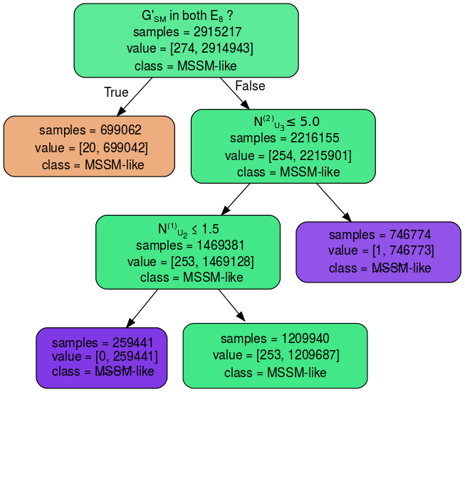
Figure 8: Decision tree on the hidden $E_{8}$ and dynamic hidden $E_{8}$ datasets from table 3, evaluated on the training set. We can extract the contrast pattern ($N_{\mathrm{U}_{2}}^{(1)}\geq 2$ and $N_{\mathrm{U}_{3}}^{(2)}\leq 5$) for MSSM-like models from this tree. One observes that this tree misclassifies one MSSM-like model after the $N_{\mathrm{U}_{3}}^{(2)}$-split in order to get better performance. See also figure 5 for further details.

Then, the decision tree is trained with the same aim as before to classify all MSSM-like models correctly in both, training and validation set. However, it turns out that this is rather difficult due to two MSSM-like models: One of these models is misclassified during training, see figure 8, the other one during validation. It turns out that these two MSSM-like models are the special $\Delta(54)$ models, where $W_{3}=W_{4}=(0^{16})$. Due to the fact that these models lie in a very specific area within the $\mathbbm{Z}_{6}$-II orbifold landscape, we decided to accept a misclassification of these models but with the benefit of obtaining a new contrast pattern that yields a further, significant reduction of the $\mathbbm{Z}_{6}$-II orbifold landscape. Doing so, we identify a new contrast pattern

$$c_{\text{U-sector}}~{}=~{}\Big{\{}N_{\mathrm{U}_{2}}^{(1)}(M)~{}\geq~{}2\;,\;N_{\mathrm{U}_{3}}^{(2)}(M)~{}\leq~{}5\Big{\}}\;,$$ (30)

for a model $M$ to have an increased probability to be MSSM-like. We call this contrast pattern U-sector as it gives bounds on the number of certain bulk matter fields, charged under the first or second $\mathrm{E}_{8}$ factor, depending on $\alpha=1,2$, respectively. Using this new constraint on top of the previous ones, the estimated growth rate reads

$$\mathrm{gr}\left(c_{\text{U-sector}},D_{\text{MSSM-like}}^{N_{\mathrm{sr}}},D_{\text{\cancel{MSSM}-like}}^{N_{\mathrm{sr}}}\right)~{}\approx~{}\dfrac{\scriptstyle{0.999}}{\tfrac{1\,209\,687}{2\,215\,901}}~{}\approx~{}1.8~{}>~{}1\;,$$ (31)

where $D^{N_{\mathrm{sr}}}$ is obtained by combining the datasets hidden $E_{8}$ and dynamic hidden $E_{8}$ from table 3. Some remarks on the subtleties of the U-sector constraints are in order:

• Contrary to the hidden $E_{8}$ contrast pattern, the U-sector contrast pattern can possibly exclude models which have $G_{\mathrm{SM}}^{\prime}$ in both $\mathrm{E}_{8}$ factors: in the case of $N_{\mathrm{sr}}^{(2)}(M)\geq 6$ models with $G_{\mathrm{SM}}^{\prime}$ in both $\mathrm{E}_{8}$ factors fulfill the even stronger condition $N_{\mathrm{sr}}^{(\alpha)}(M)\geq 8$ for $\alpha=1,2$. This can not be guaranteed for the U-sector constraint. Therefore, the growth rate in eq. (31) is estimated using only those models where $G_{\mathrm{SM}}^{\prime}$ is exclusively in the first $\mathrm{E}_{8}$ factor.

• Interestingly, the $\Delta(54)$ MSSM-like models excluded by the constraint $N_{\mathrm{U}_{3}}^{(2)}(M)\leq 5$ do obey the subsequent constraint $N_{\mathrm{U}_{2}}^{(1)}(M)\geq 2$ on the number of bulk matter from the $U_{2}$ sector and charged under the first $\mathrm{E}_{8}$. Even though the decision tree decided strictly correct (by taking the statistics into account for optimization) and misclassified these two MSSM-like models, it is still appealing that all MSSM-like models (with $G_{\mathrm{SM}}^{\prime}\in\mathrm{E}_{8}^{(1)}$) obey this constraint. This observation might be worth further investigations.

Implementing the U-sector contrast pattern into our search algorithm displayed in figure 1 and performing an intensive search (using all Wilson lines or turning off $W_{5}$ by hand), we obtain our final dataset, called U-sector, see table 3. The results show once more the strength of the contrast data mining technique applied to the heterotic orbifold landscape: The probability to find MSSM-like models has increased further as shown in figure 9 and the U-sector contrast pattern generalizes to the $\mathbbm{Z}_{6}$-II landscape such that we obtained many new inequivalent MSSM-like models. Starting from 395 inequivalent MSSM-like models in the dynamic hidden $E_{8}$ dataset we obtain now 459 models. Finally, combining all datasets yields in total 468 inequivalent MSSM-like $\mathbbm{Z}_{6}$-II models. 

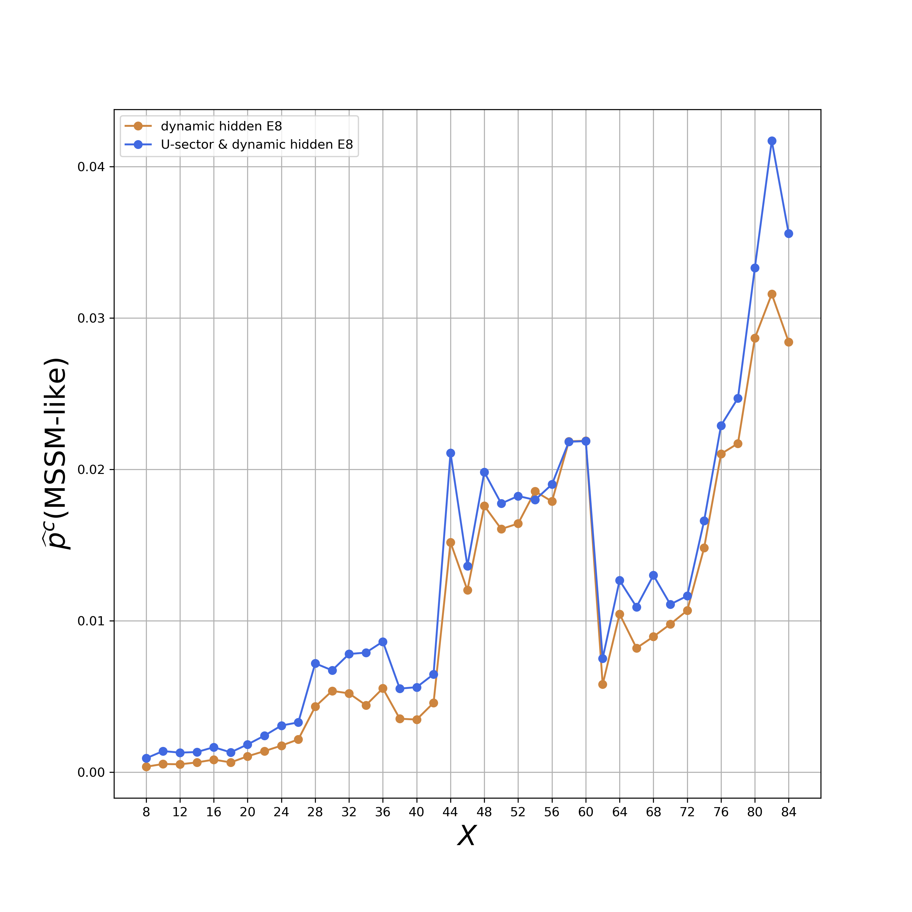
Figure 9: Comparison of two different dynamic hidden $E_{8}$ searches: (i) without and (ii) with the additional U-sector constraint. For both cases, we display the probability $\hat{p}^{c}(\text{MSSM-like})$ (estimated on the sample) to find MSSM-like models under the constraint of the respective contrast pattern $c$ as a function of the threshold value $X$, where $c$ is (i) $N_{\mathrm{sr}}^{(2)}\geq X$ and (ii) a combination of case (i) and the U-sector constraint, respectively.

To summarize, we were able to significantly exceed all previous searches for MSSM-like $\mathbbm{Z}_{6}$-II models [19, 20, 17, 18] by excluding those regions in the $\mathbbm{Z}_{6}$-II orbifold landscape where most likely no MSSM-like model exists. It is tempting to speculate that some of our contrast patterns might even be necessary conditions for all MSSM-like models. Moreover, we learned some general features of MSSM-like models that can be produced in the $\mathbbm{Z}_{6}$-II orbifold landscape: We were able to identify constraints on physical quantities that can be interpreted and analyzed directly. Later, in section 6, we will show that the hidden $E_{8}$ contrast pattern can be transferred to other orbifold geometries while the lower bound of this constraint will be sensitive to the orbifold geometry under consideration.

5 $\mathbbm{Z}_{6}$-II orbifold models with $\Delta(54)$ flavor symmetry

Out of the 468 inequivalent MSSM-like models based on the $\mathbbm{Z}_{6}$-II orbifold geometry, there are two models with vanishing Wilson lines in the $\mathbbm{Z}_{3}$ torus, i.e. $W_{3}=W_{4}=(0^{16})$. Hence, these MSSM-like models are equipped with a $\Delta(54)$ ($R$-) flavor symmetry [48, 49, 50], where localized matter fields transform in three-dimensional representations of $\Delta(54)$.

Both models are very similar. They are based on the same shift (shift No. 18 according to the enumeration of ref. [51]), but in different representations. This shift breaks the ten-dimensional $\mathrm{E}_{8}\times\mathrm{E}_{8}$ gauge group to

$$\mathrm{SO}(10)\times\mathrm{SU}(3)\times\mathrm{U}(1)\quad\mathrm{and}\quad\mathrm{SO}(12)\times\mathrm{SU}(2)\times\mathrm{U}(1)\;,$$ (32)

in the first and second $\mathrm{E}_{8}$, respectively. As a remark, this shift is different from the two local $\mathrm{SO}(10)$ shifts of ref. [19]. In a next step, $\mathrm{SO}(10)$ (and the hidden $\mathrm{SO}(12)\times\mathrm{SU}(2)$ gauge group) is broken by the Wilson lines $W_{5}$ and $W_{6}$ to the Standard Model gauge group, while the $\mathrm{SU}(3)$ factor remains unbroken as additional gauged $\mathrm{SU}(3)_{\mathrm{flavor}}$ flavor symmetry (Hence, the full flavor symmetry is actually $\mathrm{SU}(3)_{\mathrm{flavor}}\times\Delta(54)$). Consequently, both models share the same four-dimensional observable gauge group originating from the first $\mathrm{E}_{8}$ factor, i.e.

$$\mathrm{SU}(3)_{\mathrm{flavor}}\times\mathrm{SU}(3)_{\mathrm{C}}\times\mathrm{SU}(2)_{\mathrm{L}}\times\mathrm{U}(1)_{Y}\times\mathrm{U}(1)^{2}\times\mathrm{hidden\ sector}\;.$$ (33)

Some details of these special MSSM-like $\mathbbm{Z}_{6}$-II orbifold models are given in the following.

5.1 $\Delta(54)$ MSSM #1 from the $\mathbbm{Z}_{6}$-II orbifold

The first $\mathbbm{Z}_{6}$-II model with $\Delta(54)$ flavor symmetry is defined by the shift vector

$$V=\left(\tfrac{385}{12},\tfrac{103}{12},\tfrac{89}{12},\tfrac{55}{12},\tfrac{15}{4},\tfrac{41}{12},\tfrac{13}{4},\tfrac{7}{12}\right),\left(\tfrac{145}{4},\tfrac{139}{12},\tfrac{33}{4},\tfrac{25}{4},\tfrac{47}{12},\tfrac{11}{4},\tfrac{7}{4},-\tfrac{7}{4}\right)\;,$$ (34)

the Wilson lines $W_{3}=W_{4}=(0^{16})$, and

$$W_{5} = \left(\tfrac{17}{2},5,2,-1,1,\tfrac{5}{2},-1,-2\right),\left(5,1,-1,0,1,\tfrac{1}{2},0,\tfrac{3}{2}\right)\;,$$ (35a)

$$W_{6} = \left(\tfrac{1}{2},-\tfrac{3}{2},-\tfrac{1}{2},3,2,\tfrac{3}{2},0,1\right),\left(2,-\tfrac{3}{2},\tfrac{1}{2},-1,2,\tfrac{7}{2},0,-\tfrac{7}{2}\right)\;.$$ (35b)

It is called MSSM431 in the model-file “Z6-II_1_1.txt” [36] that can be loaded to the orbifolder. For his model, the hidden gauge group is broken to

$$\mathrm{SU}(3)\times\mathrm{SU}(3)\times\mathrm{U}(1)^{4}\;.$$ (36)

The massless string spectrum is summarized in table 6. Interestingly, the spectrum contains flavons that are triplets under both $\Delta(54)$ and $\mathrm{SU}(3)_{\mathrm{flavor}}$. Hence, their vacuum expectation values could break the full flavor group to a diagonal subgroup.

#	irrep	labels	#	irrep	labels
6	$\left(\boldsymbol{1};\boldsymbol{3},\boldsymbol{2};\boldsymbol{1},\boldsymbol{1}\right)_{-\tfrac{1}{6}}$	$q_{i}$	3	$\left(\boldsymbol{1};\bar{\boldsymbol{3}},\boldsymbol{2};\boldsymbol{1},\boldsymbol{1}\right)_{\tfrac{1}{6}}$	$\bar{q}_{i}$
1	$\left(\boldsymbol{3};\bar{\boldsymbol{3}},\boldsymbol{1};\boldsymbol{1},\boldsymbol{1}\right)_{\tfrac{2}{3}}$	$\bar{u}_{i}$
1	$\left(\bar{\boldsymbol{3}};\bar{\boldsymbol{3}},\boldsymbol{1};\boldsymbol{1},\boldsymbol{1}\right)_{-\tfrac{1}{3}}$	$\bar{d}_{i}$
5	$\left(\boldsymbol{1};\bar{\boldsymbol{3}},\boldsymbol{1};\boldsymbol{1},\boldsymbol{1}\right)_{-\tfrac{1}{3}}$	$\bar{d}_{i}$	5	$\left(\boldsymbol{1};\boldsymbol{3},\boldsymbol{1};\boldsymbol{1},\boldsymbol{1}\right)_{\tfrac{1}{3}}$	$d_{i}$
10	$\left(\boldsymbol{1};\boldsymbol{1},\boldsymbol{2};\boldsymbol{1},\boldsymbol{1}\right)_{\tfrac{1}{2}}$	$\ell_{i}$	7	$\left(\boldsymbol{1};\boldsymbol{1},\boldsymbol{2};\boldsymbol{1},\boldsymbol{1}\right)_{-\tfrac{1}{2}}$	$\bar{\ell}_{i}$
1	$\left(\boldsymbol{3};\boldsymbol{1},\boldsymbol{1};\boldsymbol{1},\boldsymbol{1}\right)_{-1}$	$\bar{e}_{1}$
12	$\left(\boldsymbol{1};\boldsymbol{1},\boldsymbol{1};\boldsymbol{1},\boldsymbol{1}\right)_{\tfrac{1}{2}}$	$s_{i}^{+}$	12	$\left(\boldsymbol{1};\boldsymbol{1},\boldsymbol{1};\boldsymbol{1},\boldsymbol{1}\right)_{-\tfrac{1}{2}}$	$s_{i}^{-}$
4	$\left(\boldsymbol{1};\boldsymbol{1},\boldsymbol{1};\boldsymbol{1},\bar{\boldsymbol{3}}\right)_{\tfrac{1}{2}}$	$s_{i}^{+}$	2	$\left(\boldsymbol{1};\boldsymbol{1},\boldsymbol{1};\boldsymbol{1},\boldsymbol{3}\right)_{-\tfrac{1}{2}}$	$s_{i}^{-}$
2	$\left(\boldsymbol{1};\boldsymbol{1},\boldsymbol{1};\boldsymbol{1},\boldsymbol{3}\right)_{\tfrac{1}{2}}$	$s_{i}^{+}$	4	$\left(\boldsymbol{1};\boldsymbol{1},\boldsymbol{1};\boldsymbol{1},\bar{\boldsymbol{3}}\right)_{-\tfrac{1}{2}}$	$s_{i}^{-}$
4	$\left(\boldsymbol{1};\boldsymbol{1},\boldsymbol{1};\bar{\boldsymbol{3}},\boldsymbol{1}\right)_{\tfrac{1}{2}}$	$s_{i}^{+}$	2	$\left(\boldsymbol{1};\boldsymbol{1},\boldsymbol{1};\boldsymbol{3},\boldsymbol{1}\right)_{-\tfrac{1}{2}}$	$s_{i}^{-}$
2	$\left(\boldsymbol{1};\boldsymbol{1},\boldsymbol{1};\boldsymbol{3},\boldsymbol{1}\right)_{\tfrac{1}{2}}$	$s_{i}^{+}$	4	$\left(\boldsymbol{1};\boldsymbol{1},\boldsymbol{1};\bar{\boldsymbol{3}},\boldsymbol{1}\right)_{-\tfrac{1}{2}}$	$s_{i}^{-}$
11	$\left(\bar{\boldsymbol{3}};\boldsymbol{1},\boldsymbol{1};\boldsymbol{1},\boldsymbol{1}\right)_{0}$	$f_{i}$	10	$\left(\boldsymbol{3};\boldsymbol{1},\boldsymbol{1};\boldsymbol{1},\boldsymbol{1}\right)_{0}$	$\bar{f}_{i}$
17	$\left(\boldsymbol{1};\boldsymbol{1},\boldsymbol{1};\boldsymbol{1},\boldsymbol{1}\right)_{0}$	$s_{i}^{0}$
7	$\left(\boldsymbol{1};\boldsymbol{1},\boldsymbol{1};\boldsymbol{3},\boldsymbol{1}\right)_{0}$	$s_{i}^{0}$	6	$\left(\boldsymbol{1};\boldsymbol{1},\boldsymbol{1};\bar{\boldsymbol{3}},\boldsymbol{1}\right)_{0}$	$s_{i}^{0}$
7	$\left(\boldsymbol{1};\boldsymbol{1},\boldsymbol{1};\boldsymbol{1},\boldsymbol{3}\right)_{0}$	$s_{i}^{0}$	6	$\left(\boldsymbol{1};\boldsymbol{1},\boldsymbol{1};\boldsymbol{1},\bar{\boldsymbol{3}}\right)_{0}$	$s_{i}^{0}$
1	$\left(\boldsymbol{1};\boldsymbol{1},\boldsymbol{1};\bar{\boldsymbol{3}},\boldsymbol{3}\right)_{0}$	$s_{i}^{0}$	1	$\left(\boldsymbol{1};\boldsymbol{1},\boldsymbol{1};\boldsymbol{3},\bar{\boldsymbol{3}}\right)_{0}$	$s_{i}^{0}$
1	$\left(\boldsymbol{1};\boldsymbol{1},\boldsymbol{1};\boldsymbol{3},\boldsymbol{3}\right)_{0}$	$s_{i}^{0}$

Table 6: Massless matter spectrum of the first $\mathbbm{Z}_{6}$-II model with $\Delta(54)$ flavor symmetry. Many SM matter fields build three-dimensional representations of $\Delta(54)$: For instance, all 6 quark-doublets $q_{i}$ combine to two three-dimensional representations of $\Delta(54)$, similar for all partners $\bar{q}_{i}$, 6 out of 10 lepton-doublets (or down-Higgs) $\ell_{i}$, and 3 out of 7 anti-lepton-doublets (or up-Higgs) $\bar{\ell}_{i}$. Furthermore, several SM singlets $s_{i}^{0}$ are three-dimensional representations of $\Delta(54)$. Finally, the SM singlets $f_{i}$ and $\bar{f}_{i}$ are flavons of $\mathrm{SU}(3)_{\mathrm{flavor}}$ (interestingly, some of these flavons are simultaneously triplets of $\Delta(54)$).

5.2 $\Delta(54)$ MSSM #2 from the $\mathbbm{Z}_{6}$-II orbifold

The second $\mathbbm{Z}_{6}$-II model with $\Delta(54)$ flavor symmetry is given by the shift vector

$$V=\left(\tfrac{247}{4},\tfrac{69}{4},\tfrac{61}{4},\tfrac{137}{12},\tfrac{101}{12},\tfrac{65}{12},\tfrac{11}{4},-\tfrac{1}{4}\right)\left(\tfrac{167}{3},\tfrac{83}{6},\tfrac{34}{3},\tfrac{55}{6},\tfrac{47}{6},\tfrac{29}{6},\tfrac{13}{6},\tfrac{1}{6}\right)\;,$$ (37)

the Wilson lines $W_{3}=W_{4}=(0^{16})$, and

$$W_{5} = \left(34,\tfrac{19}{2},\tfrac{15}{2},\tfrac{11}{2},\tfrac{11}{2},\tfrac{7}{2},\tfrac{1}{2},-3\right)\left(-\tfrac{113}{4},-\tfrac{23}{4},-\tfrac{17}{4},-\tfrac{13}{4},-\tfrac{27}{4},-\tfrac{17}{4},-\tfrac{3}{4},\tfrac{5}{4}\right)\;,$$ (38a)

$$W_{6} = \left(-\tfrac{11}{4},-\tfrac{1}{4},\tfrac{5}{4},-\tfrac{7}{4},-\tfrac{11}{4},\tfrac{1}{4},-\tfrac{1}{4},-\tfrac{11}{4}\right)\left(16,1,3,2,4,\tfrac{5}{2},-\tfrac{1}{2},-2\right)\;.$$ (38b)

It is called MSSM438 in the model-file “Z6-II_1_1.txt” [36]. In this case, the hidden gauge group is broken to

$$\mathrm{SU}(5)\times\mathrm{U}(1)^{4}\;,$$ (39)

in four dimensions and the massless string spectrum is given in table 10 in appendix A. Compared to the $\Delta(54)$ MSSM #1, $\mathrm{SU}(3)_{\mathrm{flavor}}$ and $\Delta(54)$ seem to have interchanged their role for many representations of quarks and leptons.

6 Geometry-dependent contrast patterns

The results from the previous sections were developed in the $\mathbbm{Z}_{6}$-II $(1,1)$ orbifold geometry. However, the basic insights from this analysis can be transferred easily to other orbifold geometries. Foremost, the concept of a hidden $E_{8}$ contrast pattern can be applied directly to other orbifold geometries: The number of unbroken roots from the hidden $\mathrm{E}_{8}$ is computed identically for all orbifold geometries and does not depend on some unknown sorting. Unfortunately, this is not given for the U-sector contrast pattern: The number of bulk matter fields $N_{\mathrm{U}_{a}}^{(\alpha)}$ for $a=1,2,3$ depends on the twist vectors of a given orbifold geometry, see eq. (19). Then, the sorting of $N_{\mathrm{U}_{1}}^{(\alpha)}$, $N_{\mathrm{U}_{2}}^{(\alpha)}$ and $N_{\mathrm{U}_{3}}^{(\alpha)}$ is determined by the sorting of the entries in the twist vectors, which is typically sorted from from small to large rotation angles. However, it is not clear why a particular U-sector might be special among the different sectors, i.e. if a special status of an U-sector is related to the sorting or to some nontrivial relation between all sectors.

Therefore, we begin with the dynamic hidden $E_{8}$ search and analyze the U-sector later. In order to apply the dynamic hidden $E_{8}$ contrast pattern to all $\mathbbm{Z}_{N}$ orbifold geometries, we first have to identify the lower bound of $N_{\mathrm{sr}}^{(2)}(M)$ (being 6 in eq. (27)) for each $\mathbbm{Z}_{N}$ orbifold geometry $\mathbbm{O}$. Thus, we define

$$X_{\mathrm{min}}(\mathbbm{O})~{}=~{}\mathrm{min}\left(\Big{\{}N_{\mathrm{sr}}^{(2)}(M)\ \Big{|}\ M\in D_{(\mathbbm{O}\text{ from \cite[cite]{[\@@bibref{}{Nilles:2014owa,Olguin-Trejo:2018wpw}{}{}]}})}\Big{\}}\right)\;.$$ (40)

To compute these bounds, we use the traditional searches of refs. [17, 18] as a background search and split the combined dataset into datasets $D_{(\mathbbm{O}\text{ from \cite[cite]{[\@@bibref{}{Nilles:2014owa,Olguin-Trejo:2018wpw}{}{}]}})}$ corresponding to the different $\mathbbm{Z}_{N}$ orbifold geometries $\mathbbm{O}$. Then, the conventional search in refs. [17, 18] can be seen as a search with $N_{\mathrm{sr}}^{(2)}\geq 0$ in our approach. Thus, we can analyze the results of the traditional search [17, 18] to obtain the lower bounds $X_{\mathrm{min}}(\mathbbm{O})$ for all $\mathbbm{Z}_{N}$ orbifold geometries. The results are stated in table 7. Moreover, the background datasets $D_{(\mathbbm{O}\text{ from \cite[cite]{[\@@bibref{}{Nilles:2014owa,Olguin-Trejo:2018wpw}{}{}]}})}$ allow us to focus the dynamic hidden $E_{8}$ contrast pattern on thresholds greater than $X_{\mathrm{min}}(\mathbbm{O})$, i.e. $N_{\mathrm{sr}}^{(2)}>X_{\mathrm{min}}(\mathbbm{O})$, in order to save computational resources in our search.

orbifold	$\mathbbm{Z}_{4}$	$\mathbbm{Z}_{6}$-I	$\mathbbm{Z}_{6}$-II	$\mathbbm{Z}_{7}$	$\mathbbm{Z}_{8}$-I			$\mathbbm{Z}_{8}$-II		$\mathbbm{Z}_{12}$-I	$\mathbbm{Z}_{12}$-II
geometry $\mathbbm{O}$	all	all	all	(1,1)	(1,1)	(2,1)	(3,1)	(1,1)	(2,1)	all	(1,1)
$X_{\mathrm{min}}(\mathbbm{O})$	4	12	6	56	6	6	4	0	4	4	6

Table 7: Lower bounds $X_{\mathrm{min}}(\mathbbm{O})$ on the number $N_{\mathrm{sr}}^{(2)}$ of unbroken roots from the hidden $\mathrm{E}_{8}$ factor for MSSM-like orbifold models from refs. [17, 18] for various $\mathbbm{Z}_{N}$ orbifold geometries $\mathbbm{O}$ (where “all” refers to the various lattices for a given $\mathbbm{Z}_{N}$ orbifold geometry, as given in the first column of table 8.).

First, let us state the results of our search in table 8: For each $\mathbbm{Z}_{N}$ orbifold geometry, we give the numbers of inequivalent MSSM-like orbifold models that we found using our dynamic hidden $E_{8}$ contrast pattern and compare these numbers to the literature. Several remarks are in order.

inequivalent MSSM-like orbifold models
orbifold		# MSSM-like	# MSSM-like	# MSSM-like using	# MSSM-like
geometry		from [17]	from [18]	contrast patterns	‘merged’
$\mathbbm{Z}_{4}$	(2,1)	128	138	125	179
	(3,1)	25	26	33	33
$\mathbbm{Z}_{6}$-I	(1,1)	31	30	31	31
	(2,1)	31	30	31	31
$\mathbbm{Z}_{6}$-II	(1,1)	348	363	468	481
	(2,1)	338	349	395	443
	(3,1)	350	351	415	482
	(4,1)	334	354	407	464
$\mathbbm{Z}_{7}$	(1,1)	0	1	1	1
$\mathbbm{Z}_{8}$-I	(1,1)	263	256	248	271
	(2,1)	164	155	144	164
	(3,1)	387	377	408	430
$\mathbbm{Z}_{8}$-II	(1,1)	638	1 833	1 259	2 289
	(2,1)	260	489	349	555
$\mathbbm{Z}_{12}$-I	(1,1)	365	556	610	625
	(2,1)	385	554	607	625
$\mathbbm{Z}_{12}$-II	(1,1)	211	352	365	435

Table 8: Table of inequivalent MSSM-like orbifold models for all $\mathbbm{Z}_{N}$ orbifold geometries, see also [36]. Note that the numbers of MSSM-like orbifold models listed in the third column differ from those in ref. [18]. This is due to an improvement of the orbifolder which has led to a better comparison of models and identified some duplicates in these sets. The last column, gives our final results: the numbers of inequivalent MSSM-like orbifold models obtained by merging the three datasets of the previous columns.

One can observe that the dynamic hidden $E_{8}$ search was able to find many new inequivalent MSSM-like orbifold models in almost all orbifold geometries. Foremost, the different $\mathbbm{Z}_{6}$-II orbifold geometries as well as the $\mathbbm{Z}_{12}$-I case have improved strongly using our contrast patterns. Note that for $\mathbbm{Z}_{6}$-II $(1,1)$, the 13 additional MSSM-like models from refs. [17, 18] fulfill all our constraints derived in section 4. Consequently, even though these models were missed in our search, they are part of our search area. Hence, these models would have been found in an extended search. A great success of our contrast patterns is also given by the appearance of the MSSM-like $\mathbbm{Z}_{7}$ model. This model was found so far only in refs. [38, 18] using an orbifold-specific search strategy, as described in appendix A of ref. [38]. Also the $\mathbbm{Z}_{6}$-I orbifold geometry is remarkable: In this case, we find a huge amount of equivalent MSSM-like models but only 31 inequivalent ones remain. These 31 inequivalent models were found very easily by searching in areas of the $\mathbbm{Z}_{6}$-I orbifold landscape with large hidden sector gauge groups, c.f. the lower bound $X_{\mathrm{min}}(\mathbbm{Z}_{6}\text{-I})=12$ given in table 7. Note that the lower bounds are computed for those models where $G_{\mathrm{SM}}^{\prime}$ appears in one $\mathrm{E}_{8}$ factor only. While most of the bounds in table 7 are weaker than $N_{\mathrm{sr}}^{(1)}\geq 8$ from section 3.2, we have to be careful in the cases of both $\mathbbm{Z}_{6}$-I orbifold geometries. There, we find a lower bound $X_{\mathrm{min}}($$\mathbbm{Z}_{6}$-I$)=12$. Thus, our search algorithm could in principle miss MSSM-like $\mathbbm{Z}_{6}$-I models where each $\mathrm{E}_{8}$ factor contains $G_{\mathrm{SM}}^{\prime}$. We analyze these problematic models separately and find a lower bound $X_{\mathrm{min}}($$\mathbbm{Z}_{6}$-I$)=10$ for these cases (because $(N_{\mathrm{sr}}^{(1)},N_{\mathrm{sr}}^{(2)})$ takes only the values $(8,12)$ and $(10,10)$ in the background dataset). This means that MSSM-like $\mathbbm{Z}_{6}$-I models which have $G_{\mathrm{SM}}^{\prime}$ in both $\mathrm{E}_{8}$ factors are contained in our search $N_{\mathrm{sr}}^{(2)}\geq 10$ for both $\mathbbm{Z}_{6}$-I orbifold geometries.

Furthermore, it seems that for some orbifold geometries like $\mathbbm{Z}_{8}$-II $(1,1)$ the conventional approach has some advantages. However, a comparison is difficult since it is not known how much computational power was invested to obtain these numbers. Moreover, for $\mathbbm{Z}_{8}$-II $(1,1)$ our contrast patterns seem to be less efficient since there is no lower bound for $N_{\mathrm{sr}}^{(2)}$, i.e. MSSM-like models with $N_{\mathrm{sr}}^{(2)}=0$ exist for $\mathbbm{Z}_{8}$-II $(1,1)$, and there are many inequivalent MSSM-like models for low values of $N_{\mathrm{sr}}^{(2)}$, which can be reached by the conventional search algorithm as well. Hence, on first sight it seems that our search algorithm is too complex for such geometries and the additional effort in computing constraints is not rewarded. However, this conclusion is premature: The merged datasets in table 8 show that our contrast patterns could still significantly improve the numbers of inequivalent MSSM-like orbifold models in these geometries. Thus, our search algorithm was able to find new MSSM-like orbifold models in corners of the landscape that were missed by the conventional approach.

On the basis of the ‘merged’ datasets we can now use decision trees to derive the U-sector constraints as in the case of the $\mathbbm{Z}_{6}$-II orbifold geometry. The results are given in table 9.

orbifold		$N_{\mathrm{U}_{1}}^{(1)}$	$N_{\mathrm{U}_{2}}^{(1)}$	$N_{\mathrm{U}_{3}}^{(1)}$	$N_{\mathrm{U}_{1}}^{(2)}$	$N_{\mathrm{U}_{2}}^{(2)}$	$N_{\mathrm{U}_{3}}^{(2)}$	gr(c)
geometry
$\mathbbm{Z}_{4}$	(2,1)			$\geq 4$			$\leq 1$	5.32
	(3,1)			$\geq 4$			$\leq 1$	6.92
$\mathbbm{Z}_{6}$-I	(1,1)	$\geq 13$		$\geq 14$				2.79
	(2,1)	$\geq 13$		$\geq 14$				2.78
$\mathbbm{Z}_{6}$-II	(1,1)		$\geq 2$				$\leq 5$	1.81
	(2,1)		$\geq 2$				$\leq 5$	1.60
	(3,1)		$\geq 2$				$\leq 5$	1.70
	(4,1)		$\geq 2$				$\leq 5$	1.86
$\mathbbm{Z}_{8}$-I	(1,1)			$\geq 4$			$\leq 25$	1.22
	(2,1)			$\geq 4$			$\leq 25$	1.23
	(3,1)			$\geq 8$				2.21
$\mathbbm{Z}_{8}$-II	(1,1)			$\geq 4$			$\leq 41$	1.61
	(2,1)			$\leq 3$			$\leq 1$	1.78
				$\geq 4$			$\leq 41$	1.01
$\mathbbm{Z}_{12}$-I	(1,1)	$\leq 10$		$\geq 2$				1.24
	(2,1)	$\leq 10$		$\geq 2$				1.24
$\mathbbm{Z}_{12}$-II	(1,1)	$\geq 2$					$\leq 5$	1.71

Table 9: U-sector constraints for various $\mathbbm{Z}_{N}$ orbifold geometries, based on the merged datasets of table 8. We neglect the $\mathbbm{Z}_{7}$ orbifold geometry because there is only one MSSM-like model available.

Let us analyze the resulting U-sector contrast patterns in some detail: In nearly all orbifold geometries it is possible to get a recall in the validation set of 1.00 and no MSSM-like model is missed in the training set. Only for the $\mathbbm{Z}_{6}$-II orbifold geometries $(1,1)$, $(2,1)$ and $(3,1)$ a very few false negative predictions were made either in the validation set or in the training set. Another special case is the $\mathbbm{Z}_{8}$-II $(2,1)$ orbifold geometry: In order to get a growth rate larger than one the decision tree had to split the set of MSSM-like models into two sets at the first node with a constraint on $N_{\mathrm{U}_{3}}^{(1)}$. Then, for both sets a second split takes $N_{\mathrm{U}_{3}}^{(2)}$ into account, resulting in a growth rate of 1.78 for the first set (containing only 3% of the MSSM-like $\mathbbm{Z}_{8}$-II $(2,1)$ models from the training set) and a growth rate of 1.01 for the second set (containing 97% of the models), respectively. In this context, let us mention that for $\mathbbm{Z}_{8}$-I $(1,1)$ it is possible to create another decision tree with a constraint ${c^{\prime}}_{\mathrm{U-sector}}=\big{\{}N_{\mathrm{U}_{3}}^{(1)}\geq 8,N_{\mathrm{U}_{3}}^{(2)}\leq 25\big{\}}$ that has a recall value of 1.00 and gr$({c^{\prime}}_{\mathrm{U-sector}})=2.18$, however, with the trade-off of missing one MSSM-like model from the training data.

Interestingly, it seems that the U-sector constraints in table 9 show some patterns on their own. Foremost, it is remarkable that for a given twist vector the exact orbifold geometry (i.e. the choice of the six-torus which is enumerated by the number $l=1,2,\ldots$ in the label $(l,1)$) does not have any significant effect. This could be used to extrapolate from one orbifold geometry to another. If the constraints are different within one twist vector one should be careful and probably take the weakest constraint, e.g. $N_{\mathrm{U}_{1}}^{(3)}\geq 4$ for $\mathbbm{Z}_{8}$-I. This can be seen as regularizing the machine learning model. One can use this insight to avoid overfitting and to use more statistics from other orbifold geometries. Additionally, one can observe that the hidden sector is completely dominated by a ‘$\leq$’ constraint in the U₃-sectors, while the visible sector favors ‘$\geq$’ (except for $\mathbbm{Z}_{12}$-I and $\mathbbm{Z}_{6}$-I). This shows that there is still more structure to explore in the heterotic orbifold landscape and, more importantly, that we are on the right track to obtain necessary conditions on both the observable $\mathrm{E}_{8}$ factor, containing the MSSM, and the hidden $\mathrm{E}_{8}$ factor.

7 Conclusion

In this paper, we have developed an advanced search strategy for MSSM-like orbifold models using the $\mathbbm{Z}_{6}$-II $(1,1)$ orbifold geometry as a test case. We obtained a significant improvement from 363 inequivalent MSSM-like models [18] to 481, see table 8. To do so, we used a technique called contrast data mining, where one identifies so-called contrast patterns that help to distinguish between MSSM-like models and others. In principle, this technique is easy to generalize to all orbifold geometries and, presumably, to other string compactifications. As a first step towards this, we analyzed all $\mathbbm{Z}_{N}$ orbifold geometries in section 6 and showed that in all cases our contrast patterns significantly enhance the known datasets of MSSM-like orbifold models, see table 8. Let us stress that this new search strategy is superior by orders of magnitudes with respect to the computing time. Theoretically, the conventional search algorithm can find all MSSM-like orbifold models. However, this would correspond to an unfeasible amount of computing time because the effort for finding a new MSSM-like model grows exponentially with the number of already constructed models. This fact was studied in detail in ref. [47] and can also be inferred from figures 3, 6 and 7. These figures show that the towers of already known orbifold models dominate the search and statistically keep growing before new orbifold models are expected to appear. Hence, with increasing search time the probability to find a new orbifold model is suppressed further and further.

Consequently, we believe that contrast patterns can be of great importance when studying the string landscape. In addition, contrast patterns are particularly useful as they have a clear physical interpretation. In our setup of heterotic orbifolds, we identified the following contrast patterns: the number of unbroken roots in the hidden $\mathrm{E}_{8}$ factor and the numbers of various bulk matter fields, charged under first or second $\mathrm{E}_{8}$ factor. Hence, our contrast patterns are related to bulk fields that originate from the compactification of the ten-dimensional $\mathrm{E}_{8}\times\mathrm{E}_{8}$ gauge bosons. Moreover, our contrast patterns have direct phenomenological implications, as they are important for supersymmetry breaking via hidden sector gaugino condensation [9, 35], gauge-Higgs unification [52, 53] and gauge-top unification [54]. Further studies along these lines have to follow.

Moreover, using the approach with contrast patterns it was possible to solve some long standing issues in the heterotic orbifold landscape, namely:

• We found many new MSSM-like orbifold models, especially in corners of the heterotic orbifold landscape that were hardly accessible by the conventional search algorithms, see table 8.

• As stated in table 3, it was possible to proof the existence of MSSM-like $\mathbbm{Z}_{6}$-II models with vanishing Wilson line of order three, i.e. $W_{3}=W_{4}=(0^{16})$. This is the first time that such models are described in the literature. They might be phenomenologically interesting as they are equipped with a $\Delta(54)$ flavor symmetry, see section 5.

• Furthermore, using the new technique we were able to reproduce the only known MSSM-like model in the $\mathbbm{Z}_{7}$ orbifold geometry [38, 18]. This model could not be found by any random search so far. Instead, it was found using a method (described in appendix A of ref. [38]) that is not feasible for most other orbifold geometries.

• Moreover, even though the main aim of our search algorithm is to find inequivalent MSSM-like orbifold models, we obtain in addition an important byproduct: our contrast patterns significantly increase the probability to find MSSM-like orbifold models in certain regions of the heterotic orbifold landscape. In future applications, the models that are classified as inequivalent by the orbifolder may differ in some other aspects, e.g. in their Yukawa couplings, see section 2.2. As soon as a preferred MSSM-like orbifold model is identified, our search algorithm allows to explore a specific part of the landscape in order to find models that have similar spectra but are not necessarily equivalent with respect to the full model.

• Also this work can be seen to be a fundamental step in applying further machine learning techniques to the heterotic orbifold landscape. In this paper, we are fighting the imbalance of the string theory datasets, i.e. we are trying to get enough data of the minority class, which is build up by the MSSM-like models. Especially, deep learning techniques are very sensible to unbalanced data and tend to perform worse than traditional machine learning methods.

Finally, we want to state some preferred properties of contrast pattern that should be kept in mind when constructing new features in the future. These properties are useful for implementation as well as for the impact of a new contrast pattern. The most important property is that a new feature can be checked quickly and easily, since it will be computed several times during the successive search algorithm. In addition, it is an advantage if a contrast pattern is testable at each step of the successive construction, see figure 1. Therefore, a new feature must be a monotonically decreasing (increasing) function with respect to the successive creation of shifts and Wilson lines. Moreover, in combination with the monotonic behavior the constraint has to be a lower (upper) bound on the model. For example, the minimal number of unbroken roots is a good contrast pattern since it can only decrease at each step in figure 1 and, therefore, it is a monotonically decreasing function with a lower bound. On the other side, the maximal number of bulk fields in a certain $U$-sector can only be checked at the last step in figure 1 since this number is also a monotonically decreasing function and any subsequently chosen Wilson line can decrease this value further. Hence, even though the number of bulk fields is a monotonically decreasing function with respect to the successive creation of shifts and Wilson lines, the $U$-sector contrast pattern is given by an upper bound, which weakens this contrast pattern.

In conclusion, this paper shows that techniques from data mining and machine learning can be applied successfully to the heterotic orbifold landscape and produce practical results, i.e. novel MSSM-like models that were out of reach using all traditional approaches so far. Further investigations in this direction have to be done in order to complete the set of contrast patterns. One might speculate that contrast patterns could ultimately help to identify an analytic formula for the construction of MSSM-like models in the heterotic orbifold landscape.

8 Acknowledgements

This work was supported by the Deutsche Forschungsgemeinschaft (SFB1258). We would like to thank Saúl Ramos-Sánchez for useful discussions.

Appendix A Spectrum of $\mathbbm{Z}_{6}$-II MSSM # 2 with $\Delta(54)$ flavor symmetry

#	irrep	labels	#	irrep	labels
1	$\left(\boldsymbol{3};\bar{\boldsymbol{3}},\boldsymbol{2};\boldsymbol{1}\right)_{\tfrac{1}{6}}$	$q_{i}$
6	$\left(\boldsymbol{1};\boldsymbol{3},\boldsymbol{1};\boldsymbol{1}\right)_{-\tfrac{2}{3}}$	$\bar{u}_{i}$	3	$\left(\boldsymbol{1};\bar{\boldsymbol{3}},\boldsymbol{1};\boldsymbol{1}\right)_{\tfrac{2}{3}}$	$u_{i}$
1	$\left(\bar{\boldsymbol{3}};\boldsymbol{3},\boldsymbol{1};\boldsymbol{1}\right)_{\tfrac{1}{3}}$	$\bar{d}_{i}$
4	$\left(\boldsymbol{1};\boldsymbol{3},\boldsymbol{1};\boldsymbol{1}\right)_{\tfrac{1}{3}}$	$\bar{d}_{i}$	4	$\left(\boldsymbol{1};\bar{\boldsymbol{3}},\boldsymbol{1};\boldsymbol{1}\right)_{-\tfrac{1}{3}}$	$d_{i}$
11	$\left(\boldsymbol{1};\boldsymbol{1},\boldsymbol{2};\boldsymbol{1}\right)_{-\tfrac{1}{2}}$	$\ell_{i}$	8	$\left(\boldsymbol{1};\boldsymbol{1},\boldsymbol{2};\boldsymbol{1}\right)_{\tfrac{1}{2}}$	$\bar{\ell}_{i}$
6	$\left(\boldsymbol{1};\boldsymbol{1},\boldsymbol{1};\boldsymbol{1}\right)_{1}$	$\bar{e}_{i}$	3	$\left(\boldsymbol{1};\boldsymbol{1},\boldsymbol{1};\boldsymbol{1}\right)_{-1}$	$e_{i}$
3	$\left(\boldsymbol{1};\bar{\boldsymbol{3}},\boldsymbol{1};\boldsymbol{1}\right)_{\tfrac{1}{6}}$	$\bar{v}_{i}$	3	$\left(\boldsymbol{1};\boldsymbol{3},\boldsymbol{1};\boldsymbol{1}\right)_{-\tfrac{1}{6}}$	$v_{i}$
12	$\left(\boldsymbol{1};\boldsymbol{1},\boldsymbol{1};\boldsymbol{1}\right)_{\tfrac{1}{2}}$	$s_{i}^{+}$	3	$\left(\bar{\boldsymbol{3}};\boldsymbol{1},\boldsymbol{1};\boldsymbol{1}\right)_{-\tfrac{1}{2}}$	$s_{i}^{-}$
2	$\left(\bar{\boldsymbol{3}};\boldsymbol{1},\boldsymbol{1};\boldsymbol{1}\right)_{\tfrac{1}{2}}$	$s_{i}^{+}$	3	$\left(\boldsymbol{3};\boldsymbol{1},\boldsymbol{1};\boldsymbol{1}\right)_{-\tfrac{1}{2}}$	$s_{i}^{i}$
15	$\left(\boldsymbol{1};\boldsymbol{1},\boldsymbol{2};\boldsymbol{1}\right)_{0}$	$m_{i}$
2	$\left(\boldsymbol{1};\boldsymbol{1},\boldsymbol{2};\boldsymbol{5}\right)_{0}$	$m_{i}$	1	$\left(\boldsymbol{1};\boldsymbol{1},\boldsymbol{2};\bar{\boldsymbol{5}}\right)_{0}$	$m_{i}$
25	$\left(\boldsymbol{1};\boldsymbol{1},\boldsymbol{1};\boldsymbol{1}\right)_{0}$	$s_{i}^{0}$
11	$\left(\bar{\boldsymbol{3}};\boldsymbol{1},\boldsymbol{1};\boldsymbol{1}\right)_{0}$	$\bar{f}_{i}$	10	$\left(\boldsymbol{3};\boldsymbol{1},\boldsymbol{1};\boldsymbol{1}\right)_{0}$	$f_{i}$
7	$\left(\boldsymbol{1};\boldsymbol{1},\boldsymbol{1};\bar{\boldsymbol{5}}\right)_{0}$	$s_{i}^{0}$	6	$\left(\boldsymbol{1};\boldsymbol{1},\boldsymbol{1};\boldsymbol{5}\right)_{0}$	$s_{i}^{0}$
2	$\left(\boldsymbol{1};\boldsymbol{1},\boldsymbol{1};\bar{\boldsymbol{10}}\right)_{0}$	$s_{i}^{0}$	1	$\left(\boldsymbol{1};\boldsymbol{1},\boldsymbol{1};\boldsymbol{10}\right)_{0}$	$s_{i}^{0}$

Table 10: Massless matter spectrum of the second $\mathbbm{Z}_{6}$-II model with $\Delta(54)$ flavor symmetry. Many SM matter fields build three-dimensional representations of $\Delta(54)$: For instance, all 6 up-quarks $\bar{u}_{i}$ combine to two three-dimensional representations of $\Delta(54)$. Furthermore, several SM singlets $s_{i}^{0}$ are three-dimensional representations of $\Delta(54)$. Finally, the SM singlets $f_{i}$ and $\bar{f}_{i}$ are flavons of $\mathrm{SU}(3)_{\mathrm{flavor}}$ (interestingly, some of these flavons are simultaneously triplets of $\Delta(54)$).

References

- [1] W. Lerche, D. Lüst, and A. N. Schellekens, Nucl. Phys. B287 (1987), 477.
- [2] M. R. Douglas, JHEP 05 (2003), 046, hep-th/0303194.
- [3] L. J. Dixon, J. A. Harvey, C. Vafa, and E. Witten, Nucl. Phys. B261 (1985), 678, [,678(1985)].
- [4] L. J. Dixon, J. A. Harvey, C. Vafa, and E. Witten, Nucl. Phys. B274 (1986), 285.
- [5] A. E. Faraggi, Nucl. Phys. B387 (1992), 239, arXiv:hep-th/9208024 [hep-th].
- [6] T. P. T. Dijkstra, L. R. Huiszoon, and A. N. Schellekens, Nucl. Phys. B710 (2005), 3, arXiv:hep-th/0411129 [hep-th].
- [7] V. Braun, Y.-H. He, B. A. Ovrut, and T. Pantev, Phys. Lett. B618 (2005), 252, arXiv:hep-th/0501070 [hep-th].
- [8] F. Gmeiner, R. Blumenhagen, G. Honecker, D. Lüst, and T. Weigand, JHEP 01 (2006), 004, arXiv:hep-th/0510170 [hep-th].
- [9] K. R. Dienes, Phys. Rev. D73 (2006), 106010, arXiv:hep-th/0602286 [hep-th].
- [10] R. Blumenhagen, B. Körs, D. Lüst, and S. Stieberger, Phys. Rept. 445 (2007), 1, arXiv:hep-th/0610327 [hep-th].
- [11] L. B. Anderson, J. Gray, A. Lukas, and E. Palti, Phys. Rev. D84 (2011), 106005, arXiv:1106.4804 [hep-th].
- [12] L. B. Anderson, J. Gray, A. Lukas, and E. Palti, JHEP 06 (2012), 113, arXiv:1202.1757 [hep-th].
- [13] M. Cvetič, D. Klevers, D. K. Mayorga Peña, P.-K. Oehlmann, and J. Reuter, JHEP 08 (2015), 087, arXiv:1503.02068 [hep-th].
- [14] M. Cvetič, L. Lin, M. Liu, and P.-K. Oehlmann, JHEP 09 (2018), 089, arXiv:1807.01320 [hep-th].
- [15] M. Cvetič, J. Halverson, L. Lin, M. Liu, and J. Tian, Phys. Rev. Lett. 123 (2019), no. 10, 101601, arXiv:1903.00009 [hep-th].
- [16] S. Groot Nibbelink and O. Loukas, JHEP 12 (2013), 044, arXiv:1308.5145 [hep-th].
- [17] H. P. Nilles and P. K. S. Vaudrevange, Mod. Phys. Lett. A30 (2015), no. 10, 1530008, arXiv:1403.1597 [hep-th].
- [18] Y. Olguin-Trejo, R. Pérez-Martínez, and S. Ramos-Sánchez, Phys. Rev. D98 (2018), no. 10, 106020, arXiv:1808.06622 [hep-th].
- [19] O. Lebedev, H. P. Nilles, S. Raby, S. Ramos-Sánchez, M. Ratz, P. K. S. Vaudrevange, and A. Wingerter, Phys. Lett. B645 (2007), 88, arXiv:hep-th/0611095 [hep-th].
- [20] O. Lebedev, H. P. Nilles, S. Ramos-Sánchez, M. Ratz, and P. K. S. Vaudrevange, Phys. Lett. B668 (2008), 331, arXiv:0807.4384 [hep-th].
- [21] D. K. Mayorga Peña, H. P. Nilles, and P.-K. Oehlmann, JHEP 12 (2012), 024, arXiv:1209.6041 [hep-th].
- [22] Y.-H. He, arXiv:1706.02714 [hep-th].
- [23] D. Krefl and R.-K. Seong, Phys. Rev. D96 (2017), no. 6, 066014, arXiv:1706.03346 [hep-th].
- [24] F. Ruehle, JHEP 08 (2017), 038, arXiv:1706.07024 [hep-th].
- [25] J. Carifio, J. Halverson, D. Krioukov, and B. D. Nelson, JHEP 09 (2017), 157, arXiv:1707.00655 [hep-th].
- [26] Y.-N. Wang and Z. Zhang, JHEP 08 (2018), 009, arXiv:1804.07296 [hep-th].
- [27] K. Bull, Y.-H. He, V. Jejjala, and C. Mishra, Phys. Lett. B785 (2018), 65, arXiv:1806.03121 [hep-th].
- [28] D. Klaewer and L. Schlechter, Phys. Lett. B789 (2019), 438, arXiv:1809.02547 [hep-th].
- [29] J. Halverson, B. Nelson, and F. Ruehle, JHEP 06 (2019), 003, arXiv:1903.11616 [hep-th].
- [30] A. Cole and G. Shiu, JHEP 03 (2019), 054, arXiv:1812.06960 [hep-th].
- [31] A. Cole, A. Schachner, and G. Shiu, arXiv:1907.10072 [hep-th].
- [32] K. Bull, Y.-H. He, V. Jejjala, and C. Mishra, Phys. Lett. B795 (2019), 700, arXiv:1903.03113 [hep-th].
- [33] A. Ashmore, Y.-H. He, and B. Ovrut, arXiv:1910.08605 [hep-th].
- [34] A. Mütter, E. Parr, and P. K. S. Vaudrevange, Nucl. Phys. B940 (2019), 113, arXiv:1811.05993 [hep-th].
- [35] O. Lebedev, H.-P. Nilles, S. Raby, S. Ramos-Sánchez, M. Ratz, P. K. S. Vaudrevange, and A. Wingerter, Phys. Rev. Lett. 98 (2007), 181602, arXiv:hep-th/0611203 [hep-th].
- [36] E. Parr and P. K. S. Vaudrevange, The model-files for the orbifolder, which contain the gauge embeddings of all MSSM-like orbifold models, can be found as arXiv ancillary files of this paper, 2019.
- [37] M. Fischer, M. Ratz, J. Torrado, and P. K. S. Vaudrevange, JHEP 01 (2013), 084, arXiv:1209.3906 [hep-th].
- [38] S. Ramos-Sánchez, Fortsch. Phys. 10 (2009), 907, arXiv:0812.3560 [hep-th], Ph.D.Thesis (Advisor: H.P. Nilles).
- [39] F. Plöger, S. Ramos-Sánchez, M. Ratz, and P. K. S. Vaudrevange, JHEP 04 (2007), 063, arXiv:hep-th/0702176 [hep-th].
- [40] H. P. Nilles, S. Ramos-Sánchez, P. K. S. Vaudrevange, and A. Wingerter, Comput. Phys. Commun. 183 (2012), 1363, arXiv:1110.5229 [hep-th], web page http://projects.hepforge.org/orbifolder/.
- [41] S. Ramos-Sánchez and P. K. S. Vaudrevange, JHEP 01 (2019), 055, arXiv:1811.00580 [hep-th].
- [42] J. Fuchs and C. Schweigert, Symmetries, Lie algebras and representations: A graduate course for physicists, Cambridge, UK: University Press, 1997, 438 p.
- [43] G. Dong and J. Bailey, Contrast data mining: Concepts, algorithms, and applications, 1st ed., Chapman & Hall/CRC, 2012.
- [44] M. Waskom, O. Botvinnik, D. O’Kane, P. Hobson, S. Lukauskas, D. C. Gemperline, T. Augspurger, Y. Halchenko, J. B. Cole, J. Warmenhoven, J. de Ruiter, C. Pye, S. Hoyer, J. Vanderplas, S. Villalba, G. Kunter, E. Quintero, P. Bachant, M. Martin, K. Meyer, A. Miles, Y. Ram, T. Yarkoni, M. L. Williams, C. Evans, C. Fitzgerald, Brian, C. Fonnesbeck, A. Lee, and A. Qalieh, mwaskom/seaborn: v0.8.1 (september 2017), September 2017.
- [45] F. Pedregosa, G. Varoquaux, A. Gramfort, V. Michel, B. Thirion, O. Grisel, M. Blondel, P. Prettenhofer, R. Weiss, V. Dubourg, J. Vanderplas, A. Passos, D. Cournapeau, M. Brucher, M. Perrot, and E. Duchesnay, Journal of Machine Learning Research 12 (2011), 2825.
- [46] C. M. Bishop, Pattern recognition and machine learning (information science and statistics), Springer-Verlag, Berlin, Heidelberg, 2006.
- [47] K. R. Dienes and M. Lennek, Phys. Rev. D75 (2007), 026008, hep-th/0610319.
- [48] T. Kobayashi, H. P. Nilles, F. Plöger, S. Raby, and M. Ratz, Nucl. Phys. B768 (2007), 135, arXiv:hep-ph/0611020 [hep-ph].
- [49] H. P. Nilles, M. Ratz, and P. K. S. Vaudrevange, Fortsch. Phys. 61 (2013), 493, arXiv:1204.2206 [hep-ph].
- [50] A. Baur, H. P. Nilles, A. Trautner, and P. K. S. Vaudrevange, arXiv:1908.00805 [hep-th].
- [51] Y. Katsuki, Y. Kawamura, T. Kobayashi, N. Ohtsubo, Y. Ono, and K. Tanioka, DPKU-8904 (1989).
- [52] L. J. Hall, Y. Nomura, and D. Tucker-Smith, Nucl. Phys. B639 (2002), 307, arXiv:hep-ph/0107331 [hep-ph].
- [53] M. Kubo, C. S. Lim, and H. Yamashita, Mod. Phys. Lett. A17 (2002), 2249, arXiv:hep-ph/0111327 [hep-ph].
- [54] P. Hosteins, R. Kappl, M. Ratz, and K. Schmidt-Hoberg, JHEP 07 (2009), 029, arXiv:0905.3323 [hep-ph].