New Quantum Structure of the Space-Time

Abstract

Abstract: Starting from quantum theory (instead of general relativity) to approach quantum gravity within a minimal setting allows us here to describe the quantum space-time structure and the quantum light cone. From the classical-quantum duality and quantum harmonic oscillator $(X,P)$ variables in global phase space we promote the space-time coordinates to quantum non-commuting operators. The phase space instanton $(X,P=iT)$ describes the hyperbolic quantum space-time structure and generates the quantum light cone. The classical Minkowski space-time null generators $X=\pm T$ dissapear at the quantum level due to the relevant quantum $[X,T]$ conmutator which is always non-zero. A new quantum Planck scale vacuum region emerges. We describe the quantum Rindler and quantum Schwarzshild-Kruskal space-time structures. The horizons and the $r=0$ space-time singularity are quantum mechanically erased. The four Kruskal regions merge inside a single quantum Planck scale ”world”. The quantum space-time structure consists of hyperbolic discrete levels of odd numbers $(X^{2}-T^{2})_{n}=(2n+1)$ (in Planck units ), $n=0,1,2...$. .($X_{n},T_{n}$) and the mass levels being $\sqrt{(2n+1)}$. A coherent picture emerges: large $n$ levels are semiclassical tending towards a classical continuum space-time. Low $n$ are quantum, the lowest mode ($n=0$) being the Planck scale. Two dual $(\pm)$ branches are present in the local variables ($\sqrt{2n+1}\pm\sqrt{2n}$) reflecting the duality of the large and small $n$ behaviours and covering the whole mass spectrum: from the largest astrophysical objects in branch (+) to the quantum elementary particles in branch (-) passing by the Planck mass. Black holes belong to both branches (+) and (-).
Norma.Sanchez@obspm.fr,    https://chalonge-devega.fr/sanchez

I Introduction and Results

Recently, we extended the known classical-quantum duality to include gravity and the Planck scale domain ref [1]. This led us to introduce more complete variables $O_{QG}$ fully taking into account all domains, classical and quantum gravity domains and their duality properties, passing by the Planck scale and the elementary particle range.

One of the results of such study is the classical-quantum duality of the Schwarzschild-Kruskal space-time.

In this paper we go further in exploring the space-time structure with quantum theory and the Planck scale domain. The classical-quantum duality including gravity and the QG variables are a key insight in this study. From the usual gravity (G) variables and quantum (Q) variables ($O_{G},O_{Q}$), we introduced QG variables $O_{QG}$ which in units of the corresponding Planck scale magnitude $o_{P}$ simply read:

$$O=\frac{1}{2}\;(\;x+\frac{1}{x}\;),\qquad O\equiv\frac{O_{QG}}{o_{P}},\qquad x\equiv\frac{O_{G}}{o_{P}}=\frac{o_{P}}{O_{Q}}$$ (1)

The $QG$ variables automatically are endowed with the symmetry

$$O(1/x)=O(x)\;\mbox{and satisfy}\;O(x=1)=1\;\mbox{at the Planck scale}.$$ (2)

QG variables are complete or global. Two values $x_{\pm}$ of the usual variables $O_{G}$ or $O_{Q}$ are necessary for each variable QG. The $(+)$ and $(-)$ branches precisely correspond to the two different and dual ways of reaching the Planck scale: from the quantum elementary particle side ($0\leq x\leq 1$) and from the classical/semiclassical gravity side ($1\leq x\leq\infty$). There is thus a classical-quantum duality between the two domains. The gravity domain is dual (in the precise sense of the wave-particle duality) of the quantum elementary particle domain through the Planck scale:

$$O_{G}=o_{P}^{2}\;O_{Q}^{-1}$$ (3)

Each of the sides of the duality Eq (1.3) accounts for only one domain: $Q$ or $G$ but not for both domains together. QG variables account for both of them, they contain the duality Eq.(1.3) and satisfy the QG duality Eq (1.2).

As the wave-particle duality, QG duality is general, it does not relate to the number of dimensions nor to any other condition.

In particular, length and time, basic QG variables $(X,T)$ in their respective Planck units are:

$$X=\frac{1}{2}\;(x+\frac{1}{x}),\quad X\;\equiv\;\frac{L_{QG}}{l_{P}}$$ (4)

$$T=\frac{1}{2}\;(\;t-\frac{1}{t}\;),\quad T\;\equiv\;\frac{T_{QG}}{t_{P}}$$ (5)

$l_{P}$ and $t_{P}$ being the Planck length and time respectively. The usual variables stand here in lowercase letters. QG mass and momemtum variables are similar to $(X,T)$:

$$P=\frac{1}{2}\;(p-\frac{1}{p}\;),\quad P\;\equiv\;\frac{P_{QG}}{p_{P}}$$ (6)

$$M=\frac{1}{2}\;(x+\frac{1}{x}),\quad M\;\equiv\;\frac{M_{QG}}{m_{P}},\quad x\equiv\frac{m}{m_{P}}$$ (7)

These are pure numbers (in Planck units), the space can be parametrized by lengths or masses. $m$ is the usual mass variable and $m_{P}$ is the Planck mass.

The complete manifold of QG variables requires several ”patches” or analytic extensions to cover the full sets $X\geq 1$ or $X\leq 1$:

$$x_{\pm}=X\pm\sqrt{X^{2}-1},\quad X\geq 1,\qquad x_{\pm}=X\pm\sqrt{1-X^{2}},\quad X\leq 1$$ (8)

The two $(X\geq 1)$, $(X\leq 1)$ domains being the classical and quantum domains respectively with their two $(\pm)$ branches each, and when $x_{+}=x_{-}$: $X=1,\;x_{\pm}=1$, (the Planck scale). The QG variables $(X,T)$ satisfy:

$$X(x)=X(1/x),\quad X(-x)=-X(x),\quad X(1)=1$$ (9)

$$T(t)=-T(1/t),\quad T(-t)=-T(t),\quad T(1)=0$$ (10)

QG variables can be also considered in phase-space ($X,P)$ with their full global analytic extension as we describe in this paper. Comparison of the QG variables with the complete Q-variables of the harmonic oscillator is enlighting, as we do in section II here.

In this paper, by promoting the QG variables $(X,T)$ to quantum non-commutative coordinates, further insight into the quantum space-time structure is obtained and new results do appear.

As already mentionned, we take quantum theory as the guide, and start by the ” prototype case”: the harmonic oscillator.

We find the quantum structure of the space-time arising from the relevant non-zero space-time commutator $[X,T]$, or non-zero quantum uncertainty $\Delta X\Delta T$ by considering quantum coordinates $(X,T)$. All other commutators are zero. The remaining transverse spatial coordinates $X_{\bot}$ have all their commutators zero.

The results of this paper are the following:

• We find the quantum light cone: It is generated by the quantum Planck hyperbolae $X^{2}-T^{2}=\pm[X,T]$ due to the quantum uncertainty $[X,T]=1$. They replace the classical light cone generators $X=\pm T$ which are quantum mechanically erased. Inside the Planck hyperbolae there is a enterely new quantum region within the Planck scale and below which is purely quantum vacuum or zero-point energy.

• In higher dimensions, the quantum commuting coordinates $(X,T)$ and the transverse non-commuting spatial coordinates $X_{\bot j}$ generate the quantum two-sheet hyperboloid $X^{2}-T^{2}+X_{\bot j}\;X_{\bot}^{j}=\pm 1$,   ${\bot}j=2,3,...(D-2)$, $D$ being the total space-time dimensions, $D=4$ in particular in the cases considered here.

• To quantize Minkowski space-time, we just consider quantum non-commutative coordinates $(X,T)$ with the usual (non deformed) canonical quantum commutator $[X,T]=1$, ($1$ is here $l_{P}^{2}$), and all other commutators zero. In light-cone coordinates

  $$U=\;\frac{1}{\sqrt{2}}\;(X-T),\qquad V=\;\frac{1}{\sqrt{2}}\;(X+T),$$

  the quadratic form (symmetric order of operators) $s^{2}=[UV+VU]=X^{2}-T^{2}=(2VU+1)$ determines the relevant part of the quantum distance. Upon identification $T=-iP$, the quantum coordinates $(U,V)$ for hyperbolic space-time are precisely the ($a,a^{+}$) operators for euclidean phase space (the phase space instanton) and as a consequence $VU$ is the Number operator. The expectation value $(s^{2})_{n}=(2n+1)$ has a minimal non zero value: $(s^{2})_{n=0}=1$ which is the zero point energy or Planck scale vacuum. Consistently, in quantum space-time:

  $$(T^{2}-X^{2})-1\geq 0:\;\mbox{{\it timelike}}$$

  $$(X^{2}-T^{2})-1\geq 0:\;\mbox{{\it spacelike}}$$

  $$(T^{2}-X^{2})-1=0,\;\mbox{{\it null}\;: the {\it"quantum light-cone"}}.$$

  This shows that only outside the null hyperbolae, that is outside the Planck scale vacuum region, such notions as distance, and timelike and spacelike signatures, can be defined, Section III and Figs 3, 4.

• Here we quantized the $(X,T)$ dimensions which are relevant to the light-cone space-time structure, as this is the case for the Rindler, Schwarzschild - Kruskal and other manifolds. The remaining spatial transverse dimensions $X_{\bot}$ are considered here as commuting coordinates. For instance, in Minkowski space-time:

  $$s^{2}=(X^{2}-T^{2}+X_{\bot j}X_{\bot}^{j}),\qquad{\bot j}=2,3,...(D-2).$$ (11)

  $$[X_{\bot j},X]=0=[X_{\bot j},T],\qquad[X_{\bot i},X_{\bot j}]=0,\qquad[P_{\bot i},P_{\bot j}]=0$$ (12)

  for all ${\bot}i,j=1,.....,(D-2)$,   $D$ being the total space-time dimensions.

  This corresponds to quantize the two-dimensional surface $(X,T)$ relevant for the light-cone structure, leaving the transverse spatial dimensions ${\bot}$ essentially unquantized (although they have zero commutators they could fluctuate). This is enough for considering the new features arising in the quantum light cone and in the quantum Rindler and the quantum Schwarzschild-Kruskal space-time structures, for which as is known, the relevant classical structures are in the $(X,T)$ dimensions and not in the transverse spatial ${\bot}$ ones. Quantum manifolds where the transverse space $X_{\bot}$ coordinates are non-commuting will be considered elsewhere.

• We find the quantum Rindler and the quantum Schwarzschild-Kruskal space-time structures. At the quantum level, the classical null horizons $X=\pm\;T$ are erased, and the $r=0$ classical singularity dissapears. The space-time structure turns out to be discretized in quantum hyperbolic levels $X_{n}^{2}-T_{n}^{2}=\pm(2n+1),\;n=0,1,2...$. For large $n$ the space-time becomes classical and continuum. Moreover, the classical singular $r=0$ hyperbolae are quantum mechanically excluded, they do not belong to any of the quantum allowed levels.

• We find the mass quantization for all masses. The quantum mass levels are associated to the quantum space-time structure. The global mass levels are $M_{n}=m_{P}\sqrt{2n+1}$   for all $n=0,1,2,...$. Two dual branches $m_{n\pm}=m_{P}\;[\sqrt{2n+1}\pm\sqrt{2n}\;]$ do appear for the usual mass variables, covering the whole mass range: from the Planck mass ($n=0$) till the largest astronomical masses: gravity branch (+), and from zero mass $(n=\infty)$ till near the Planck mass: elementary particle branch (-). For large $n$, masses increase as $m_{P}(2\sqrt{2n})$ in branch (+) while they decrease as $m_{P}/(2\sqrt{2n})$ in branch (-). For very large $n$ the spectrum becames continuum. Black holes belong to both branches (+) and (-); quantum strings have similar mass quantization. In the conclusions we comment on these aspects.

• The end of black hole evaporation is not the subject of this paper but our results here have implications for it. Black hole ends its evaporation in branch (-). We know from refs [2],[7],[8] that it decays like a quantum heavy particle in pure (non mixed) states. In its last phase (mass smaller than the Planck mass $m_{P}$), the state is not anymore like a black hole but like a heavy particle. We discuss more on it in the conclusions.

This paper is organized as follows: In Section II we describe quantum space-time as a quantum harmonic oscillator and its classical-quantum duality properties. In Section III we describe the quantum Rindler space-time and its structure. Section IV deals with the quantum Schwarzschild-Kruskal space-time and its properties. In Section V we treat the quantized whole mass spectrum. In Section VI we present our remarks and conclusions.

II Quantum Space-Time as a Harmonic Oscillator

Comparison of the QG variables to the harmonic oscillator variables is enlighting. Let us first consider the complete variables not yet promoted to quantum non-conmuting operators. The oscillator complete variables $(X,P)$ containing both the classical and quantum components are:

$$X_{Q}=\frac{l}{2}\;(\frac{l}{\hbar}\;p+\frac{\hbar}{l\;p}),\qquad P_{Q}=\frac{\hbar}{2l}\;(\frac{l}{\hbar}p-\frac{\hbar}{l\;p}\;),\qquad{l}=\frac{2\pi}{\omega}$$

being $l$ the length of the oscillator, (also expressed as $\sqrt{\hbar m/\omega}$.

Or, in dimensionless variables:

$$X=\frac{1}{2}\;(p+\frac{1}{p}),\qquad P=\;\frac{1}{2}\;(p-\frac{1}{p}),\quad p\equiv\frac{l}{\hbar}p,\qquad X\equiv\;\frac{X_{Q}}{l},\qquad P\;\equiv\frac{l}{\hbar}\;P_{Q}$$

There are two branches $p_{\pm}$ for each variable $X$ or $P$ and the two domains $X\geq 1$ and $X\leq 1$ are dual of each other, classical and quantum ones respectively:

• Classical: $X^{2}>>1$; Transition: $X^{2}\simeq 1$, $p_{+}=p_{-}=1$; Quantum: $X^{2}\leq 1$.

Or, in terms of the star variables $p=\exp p*$ :

$$X=\cosh p*,\quad P=\sinh p*,\quad X^{2}-P^{2}=1.$$

The value ${l}=1$, ie $\hbar=m\omega$, (quantum action and classical momentum equal) is here the analogous of the Planck scale for QG, ie the transition from the classical $(m\omega>>\hbar)$ regime to the quantum $(m\omega<<\hbar)$ regime. The hyperbolae $X^{2}-P^{2}=1$, or fully dimensional $X_{Q}^{2}/l^{2}-(l^{2}P_{Q}^{2})/\hbar^{2}=1,$ are the transition ”boundaries” between the classical or semiclassical and the quantum regions in the complete analytic extension of the ($X,P$) manifold. This is a hyperbolic phase space structure. Fig. 1 displays the four regions:

• Right and left exterior regions to the hyperbola $X^{2}-P^{2}=\pm 1$ , $\left|X\right|\geq P$ and $\left|X\right|\leq|P|$ are classical: $X>>1$: $m\omega>>\hbar$

• The hyperbolae $X^{2}-P^{2}=\pm 1$ are the transition boundaries $l\simeq 1:m\omega\simeq\hbar$. They separate the classical from the semiclassical and quantum regions.

• ”Future” and ”past” interior regions $P>0$ and $P<0$ are quantum: $X<<1$: $m\omega<<\hbar$

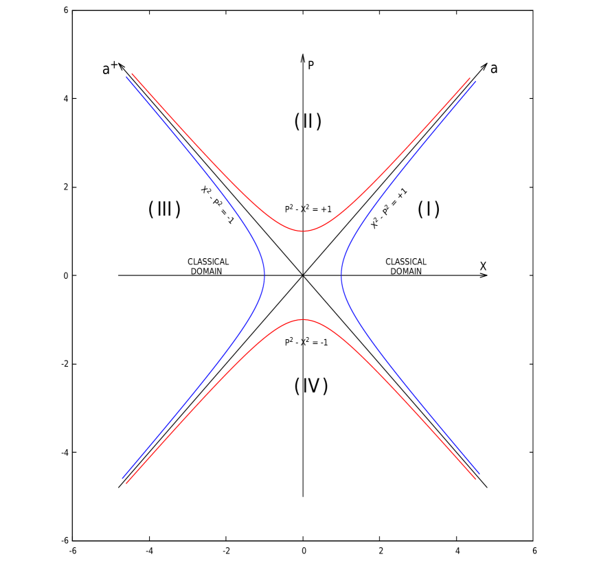
Figure 1: The complete analytic extension of the $(X,P)$ quantum harmonic oscillator variables and its classical and quantum domains: Hyperbolic phase space. The $(a,a^{+})$ operators are like light-cone coordinates. The instanton $P\rightarrow iP$, is the usual (elliptic) phase space with (dimensionless) hamiltonian $(X^{2}+P^{2})=2H$, (in units of the typical oscillator length).

Extension of $P$ to be purely imaginary: $P\rightarrow iP$, $p*\rightarrow ip*$, (ie instanton) goes from the hyperbolic to the elliptic phase space structure with the Hamiltonian $H=(X^{2}+P^{2})/2$, or in the dimensionfull variables:

$$H_{Q}=\frac{\omega\hbar}{2}\;(\frac{X_{Q}^{2}}{l^{2}}+\frac{l^{2}P_{Q}^{2}}{\hbar^{2}}),\qquad H\equiv\frac{H_{Q}}{\omega\hbar}$$

By promoting $(X,P)$ to be quantum operators, in terms of the $(a,a^{+})$ representation yields:

$$X=\;\frac{1}{\sqrt{2}}\;(a^{+}+a),\qquad P=\;\frac{i}{\sqrt{2}}\;(a^{+}-a),\qquad[a,a^{+}]=1,$$ (13)

$$2H=(X^{2}+P^{2})=(aa^{+}+a^{+}a)=2\;(a^{+}a+\frac{1}{2}),\qquad(X^{2}-P^{2})=(a^{2}+a^{+2})$$ (14)

$$[2H,P]=iX,\qquad\;[2H,X]=-iP,\qquad\;[X,P]=i,$$

$$\mbox{with the quantum levels}\;\;\epsilon_{n}=(n+\frac{1}{2}),\;\;n=0,1,...$$ (15)

These are the dimensionless levels, (otherwise they are multiplied by $\omega\hbar$).

The $(a,a^{+})$ operators are the light-cone type quantum coordinates of the phase space $(X,P)$:

$$a=\;\frac{1}{\sqrt{2}}\;(X+iP),\qquad a^{+}=\;\frac{1}{\sqrt{2}}\;(X-iP)$$ (16)

The temporal variable $T$ in the space-time configuration $(X,T)$ is like the (imaginary) momentum in phase space $(X,P)$: The identification $P=iT$ in Eqs (2.1)-(2.3) yields:

$$X=\;\frac{1}{\sqrt{2}}\;(a^{+}+a),\qquad T=\;\frac{1}{\sqrt{2}}\;(a^{+}-a),\qquad[a,a^{+}]=1,$$ (17)

$$2H=(X^{2}-T^{2})=2\;(a^{+}a+\frac{1}{2}),\;\qquad(X^{2}+T^{2})=(a^{2}+a^{+2}),$$ (18)

$$[2H,T]=X,\qquad\;[2H,X]=T,\qquad\;[X,T]=1,$$ (19)

$a^{+}\;a=N$ being the number operator.

Regions I, II, III, IV, corresponding to the exterior and interior regions to the hyperbolae $X^{2}\geq(T^{2}\pm 1)$, $X^{2}\leq(T^{2}\pm 1)$ respectively, are covered by patches similar to the (space-like) Eqs.(2.5)-(2.7). $X$ and $T$ are interchanged in the time-like regions, similar to the global hyperbolic structure Fig 1.

Given the quantum hyperbolic space-time structure above described , we can think then the quantum space-time coordinates $(X,T)$ as quantum harmonic oscillator coordinates $(X,T=iP)$, including quantum space-time fluctuations with length and mass in the Planck scale domain and quantized levels, as described by Eqs (2.5)-(2.7):

$$0\leq\;l\;\leq l_{P},\quad\epsilon_{n}=(n+\frac{1}{2}),\;\;n=1,2,...,\qquad\omega=2\pi/l$$

Expectation values of Eqs (2.6) yield

$$(X^{2}-T^{2})_{n}\;=\;2\;(n+\frac{1}{2})$$ (20)

The quantum algebra Eqs (2.5)-(2.7) describe the basic quantum space-time structure.

• When $[X,T]=0$, they yield the characteristic lines and light cones generators $X=\pm T$ of the classical space-time structure and its causal domains, (Fig.2).

• At the quantum level, the corresponding characteristic lines and light cone generators Eqs (2.6)-(2.8) are bent by the relevant $[X,T]$ commutator, they do not cross at $X=\pm T=0$ but are separated by the quantum hyperbolic region $2\epsilon_{0}$ due to the zero point energy (or quantum space-time width) $\epsilon_{0}=(1/2)[X,T]$:

  $$(X^{2}-T^{2})=\pm[X,T]=\pm 1,\;1=2\epsilon_{0},\;(n=0):\quad\mbox{the quantum light cone}$$ (21)

  $$[X,T]=0:\qquad X=\pm T:\qquad\mbox{the classical light cone}.$$

• The hyperbolae Eq.(2.9) are the quantum light cone. They quantum generalize the classical light cone $X=\pm T$ generators when $[X,T]=0$. The classical generators are the asymptotes for $T\rightarrow\pm\infty$. Quantum mechanically, $X$ is always different from $\pm T$ since $[X,T]$ is always different from zero. Figs 2-3 illustrate these properties: The well known classical (non quantum) light cone generators and the new quantum light cone (quantum Planck hyperbolae) due to the $2\epsilon_{0}$ zero-point energy.

• Quantum fluctuations and the quantum generated thickness make the space-time structure spread, and its signature or causal structure is quantum mechanically modified, entangled, or erased in the quantum Planck scale region.

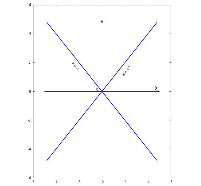
Figure 2: The classical light cone.

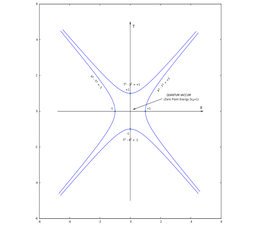
Figure 3: The quantum light cone (in units of the Planck length). It is generated by the quantum hyperbolae $T^{2}-X^{2}=\pm[X,T]=\pm 1$. For comparison, the classical limit: light cone generators $X=\pm T$, is shown in Fig. 2. A new quantum region does appear inside the four Planck scale hyperbolae: The Planck scale vacuum due to the zero-point energy $2\epsilon_{0}=1$. The four causal regions dissapear inside this Planck scale region. The classical conical vertex $X=\pm T=0$ spreaded, smeared or erased at the quantum level. This is due to the non-zero quantum commutator $[X,T]$ or $\Delta X\Delta T$ uncertainty Eqs (2.7).

The quantization condition Eq.(2.8) yields in this context the quantum levels of the space-time. The space-time hyperbolic structure is discretized in odd number levels, Fig 4. It yields for the global coordinates:

$$X_{n}=\sqrt{(2n+1)}\quad\mbox{ for all $n$ = 0, 1, 2, ... }$$

$$X_{n}\;{}_{\;\;n>>1}\;=\sqrt{2\;n}\;+\frac{1}{2\sqrt{2\;n}}+O(1/n^{3/2}),\qquad\mbox{large $n$}$$ (22)

$$X_{n}=1+n+O(n^{2}),\qquad\mbox{low $n$}$$ (23)

In terms of the local coordinates $x$ Eq.(1.4), it translates into the quantization:

$$x_{n\pm}=[\;X_{n}\pm\sqrt{X_{n}^{2}-1}\;]=[\;\sqrt{2n+1}\pm\sqrt{2n}\;]$$ (24)

The condition $X_{n}^{2}\geq 1$ simply implies $n\geq 0$: The $n=0$ value corresponds to the Planck scale $(X_{0}=1)$ :

$$x_{0+}=x_{0-}=1,\;\;n=0:\qquad\mbox{Planck scale}$$ (25)

$$x_{n\pm}=1\pm\sqrt{2\;n}\;+n+O(n^{2}),\qquad\mbox{low $n$}$$ (26)

$$x_{n+}=2\sqrt{2\;n}\;-\;\frac{1}{2\sqrt{2\;n}}+O(1/n^{3/2}),\quad x_{n-}=\frac{1}{2\sqrt{2\;n}}+O(1/n^{3/2}),\quad\mbox{large $n$}$$ (27)

Similar analysis holds for $T_{n}$ and the inverse local coordinates $t_{n\pm}$:

$$t_{n\pm}=[\;T_{n}\pm\sqrt{T_{n}^{2}+1}\;]=\sqrt{2}\;[\sqrt{2n+1}\pm\sqrt{(2n+1)+1/2}\;]$$ (28)

In the time-like regions, $X_{n}$ and $T_{n}$ are exchanged, thus covering the global quantum hyperbolic structure, as shown in Fig.4.

A coherent picture emerges:

• The large modes $n$ correspond to the semiclassical or classical states tending towards the classical continum space-time in the very large $n$ limit

• The low $n$ are quantum, with the lowest mode corresponding to the Planck scale $X_{0}=1$, $x_{0+}=x_{0}=1$.

• The two $x_{n\pm}$ values indicate the two different and dual ways of reaching the Planck scale: from the classical/semiclassical side $x_{n+}>>1$: the $(+)$ branch, and from the quantum $0\leq x_{n}\leq 1$ side: the $(-)$ branch. The large and low $n$ behaviours precisely account for these two dual classical-quantum domains.

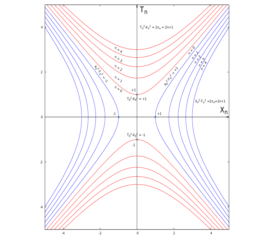
Figure 4: The quantum space-time and its hyperbolic structure. It turns out to be discretized in quantum hyperbolic levels of odd numbers (in units of the Planck length): $X_{n}^{2}-T_{n}^{2}=\pm(2n+1)$ (space-like regions), [$T_{n}^{2}-X_{n}^{2}=\pm(2n+1)$ in the timelike regions], $n=0,1,2,...$, $n=0$ being the Planck scale (zero point quantum energy). The $n=0$ quantum hyperbolae generate the quantum light cone, Fig. 3. Low $n$ levels are quantum and bent, large $n$ are classical, less bent tending asymptotically to a classical continum space-time. For comparison, the classical space time is shown in Fig.2

We see that in order to gain physical insight in the quantum Minkowski space-time structure, we can just consider quantum non-commutative coordinates $(X,T)$ with usual quantum commutator $[X,T]=1$, (1 is here $l_{P}^{2}$), and all other commutators zero. In light-cone coordinates

$$U=\;\frac{1}{\sqrt{2}}\;(X-T),\qquad V=\;\frac{1}{\sqrt{2}}\;(X+T),$$

the quadratic form (symmetric order of operators)

$$s^{2}=[UV+VU]=X^{2}-T^{2}=(2VU+1),$$ (29)

determines the relevant component of the quantum distance. This corresponds exactly to the analytic continuation of the euclidean operator $2H=(aa^{+}+a^{+}a)$. The quantum coordinates $(U,V)$ for hyperbolic space-time are the hyperbolic $(T=iP)$ operators ($a,a^{+}$) of euclidean phase space and $VU\equiv N$ is the Number operator. The expectation value $(s^{2})_{n}=(2n+1)$ has as minimal value: $(s^{2})^{1/2}_{n=0}=\pm 1$. Consistently, in quantum space-time we have:

$$(T^{2}-X^{2})-1\geq 0:\;\mbox{{\it timelike}}$$

$$(X^{2}-T^{2})-1\geq 0:\;\mbox{{\it spacelike}}$$

$$(T^{2}-X^{2})-(\pm 1)=0,\;\mbox{{\it null}, (the {\it quantum light-cone)}}.$$

This is so because only outside the null hyperbolae, ie outside the Planck vaccum region such notions as distance, and timelike and spacelike signatures can have a meaning, Figs 1, 2.

Here we quantized the $(X,T)$ dimensions which are relevant to the light-cone space-time structure. The remaining spatial transverse dimensions $X_{\bot}$ are considered here as commuting coordinates, ie having all their commutators zero. For instance, in quantum Minkowski space-time:

$$s^{2}=(X^{2}-T^{2}+X_{\bot j}X_{\bot}^{j}),\qquad{\bot j}=2,...(D-2)$$ (30)

$$[X_{\bot j},X]=0=[X_{\bot j},T],\qquad[X_{\bot i},X_{\bot j}]=0,\qquad[P_{\bot i},P_{\bot j}]=0$$ (31)

for all ${\bot}~{}i,j=1,.....,(D-2)$. $D$ being the total space-time dimensions. In particular $D=4$ in the cases considered here.

This corresponds to quantize the two-dimensional surface $(X,T)$ relevant for the light-cone structure, leaving the transverse spatial dimensions ${\bot}$ with zero commutators. This is enough for considering the new structure arising in the quantum light cone and in the quantum Rindler and quantum Schwarzschild-Kruskal space-times, for which as it is known, the relevant dimensions for the space-time structure are $(X,T)$, (and $x*,t*$) and not the transverse spatial ${\bot}$ dimensions.

This is like one harmonic oscillator in the light cone surface $(X,T)$, and no oscillator in the transverse spatial dimensions ${\bot}$. (Although the $X_{\bot j}$ variables have zero commutators, they could fluctuate).

Here we focus on the space-time quantum structure arising from the relevant non-zero conmutator $[X,T]$ and the quantum light cone. Thus, to follow on the same line of argument, we will consider below the quantum Rindler and the quantum Schwarzschild-Kruskal space-time structures. Other quantum manifolds where the transverse space $X_{\bot}$ coordinates are also non-commuting can be considered.

III Quantum Rindler-Minkowski Space-Time

The above quantum description is still more illustrative by considering the transformation:

$$X=\exp{(\kappa x*)}\;\cos(\kappa p*),\qquad P=\exp{(\kappa x*)}\;\sin(\kappa p*)$$ (32)

which is the Rindler phase space representation $(x*,p*)$ of the complete Minkowski phase space $(X,P)$. The parameter $\kappa$ is the dimensionless (in Planck units) acceleration. (Here we can express $\kappa=l_{P}/l=l_{P}\omega$). For classical, ie. non-quantum coordinates $(X,P)$ we have:

$$(X^{2}+P^{2})=\exp{(2\kappa x*)}=2\;H,\qquad(X^{2}-P^{2})=\exp{(2\kappa x*)}\;\cos(2\kappa p*)$$ (33)

We promote now $(X,P)$ to be quantum non-commuting operators, as well as $(x*,p*)$. We get:

$$(X^{2}+P^{2})=\exp{(2\kappa x*)}\;\cos(\kappa[x*,p*])$$ (34)

$$(X^{2}-P^{2})=\exp{(2\kappa x*)}\;\cos(2\kappa p*)$$ (35)

$$[X,P]=\exp{(2\kappa x*)}\;\sin(\kappa[x*,p*]),$$ (36)

where we used the usual exponential operator product:
$\exp({A})\exp({B})=\exp({B})\exp({A})\exp({[A,B]})$.

Eqs (3.3)-(3.5) describe the quantum Rindler phase space structure. The quantum Rindler space-time follows upon the identification $P=iT,p*=it*$:

$$X=\exp{(\kappa x*)}\;\cosh(\kappa t*),\qquad T=\exp{(\kappa x*)}\;\sinh(\kappa t*)$$

$$(X^{2}-T^{2})=\exp{(2\kappa x*)}\;\cosh(\kappa[x*,t*])$$ (37)

$$(X^{2}+T^{2})=\exp{(2\kappa x*)}\;\cosh(2\kappa t*)$$ (38)

$$[X,T]=\exp{(2\kappa x*)}\;\sinh(\kappa[x*,t*])$$ (39)

• We see the new terms appearing due to the quantum conmutators $[X,T]$ and $[x*,t*]$. At the classical level: $[X,T]=0$, $[x*,t*]=0$ and the known classical Rindler-Minkowski equations are recovered.

• $(X,T)$ and $(x*,t*)$ are quantum coordinates and Eqs (3.6)-(3.8) reveal the quantum structure of the Rindler-Minkowski space-time, their classical, semiclassical and quantum regions and the classical-quantum duality between them. Eqs (3.6) and (3.8) yield:

  $$(X^{2}-T^{2})=\pm\sqrt{\exp{(4\kappa x*)}+[X,T]^{2}}$$ (40)

• We see the role played by the quantum non-zero commutators. Also, if the commutators would not be c-numbers, the r.h.s. of Eqs (3.6)-(3.8) would be just the first terms of the exponential operator expansions, but this does not affect the general conclusions here. From Eqs (3.6)-(3.8), expectations values and quantum dispersions can be obtained.

• Eq (3.9) quantum generalize the classical space-time Rindler ”trajectories”:

  $$(X^{2}-T^{2})_{classical}=\exp{(2\kappa x*)},\qquad[X,T]=0\;\mbox{\it{classically}}$$ (41)

  The quantum analogue of the trajectories ($x*$ = constant) are bendt by the non-zero commutator (quantum uncertainty or quantum width) as well as the generating Rindler’s light-cone. The classical Rindler’s horizons $(x*=-\infty)$ $X=\pm T$ are quantum mechanically erased, replaced by

  $$(X^{2}-T^{2})=\pm\;[X,T]=\pm\;1:\;\;\;\mbox{{\it quantum} Planck scale hyperbolae,}$$ (42)

  which are the quantum ”light cone”. At the quantum level, the classical null generators $X=\pm T$ spread and disappear near and inside the quantum Planck scale vacuum region Eqs (2.9), Fig (3)

• The quantum algebra Eqs (3.6)-(3.8) and the quantum dispersions and fluctuations imply that the four space-time regions (classically I, II, III, IV), are spreaded or ”fuzzy”, entangled or erased at the quantum level, near and inside the Planck domain delimitated by the four Planck scale hyperbolae Eq (3.11), Figs 3 and 4.

• Fig 4 shows the quantum discrete levels of Minkowski-Rindler space-time and all the previous discussion applies here

  $$X_{n}^{2}-T_{n}^{2}=\pm(2n+1),\qquad n=0,1,2,...$$ (43)

  ”Exterior” Rindler regions to the Planck scale hyperbolaes $(X^{2}-T^{2})_{n=0}$ = $\pm 1$ contain the quantum, semiclassical and classical behaviours, from $n=0$ and the low $n$ to the large ones, which became more classical and less bendt, in agreement with the classical-quantum duality of space-time structure.

• The interior region to the $n=0$ levels is the full quantum Planck scale domain. The ”future” and ”past” regions are composed by levels from the very quantum (the Planck $n=0$ hyperbolae and low $n$), to the semiclassical and classical (large $n$) levels $(X_{n},T_{n})$.

• The Rindler levels $(x*_{n\pm},t*_{n\pm})$ follow from Eqs (2.13)-(2.17) for $(x_{n\pm},t_{n\pm})$:

  $$x_{n\pm}=\exp{(\kappa x*_{n\pm})}=[\;X_{n}\pm\sqrt{X_{n}^{2}-1}\;]=[\;\sqrt{2n+1}\pm\sqrt{2n}\;]$$ (44)

  $$t_{n\pm}=\exp{(\kappa t*_{n\pm})}=[\;T_{n}\pm\sqrt{T_{n}^{2}+1}\;]=[\sqrt{2n+1}\pm\sqrt{(2n+1)+1/2}\;]$$ (45)

• Due to the quantum space-time width, quantum light-cone or quantum dispersion and fluctuations, and the quantum Planck scale nature of the interior region, the difference between the four causal regions I, II, III, IV is quantum mechanically erased in the Planck scale region. The classical copies or halves (I, II) and (III, IV) became one only quantum world.

• This provides further support to the antipodal identification of the two space-time copies which are classically or semiclassically the space and time reflections of each other and which are classical-quantum duals of each other, and therefore supports the antipodally symmetric quantum theory, refs [3], [4], [5], [6]. The classical/semiclassical antipodal space-time symmetry and the CPT symmetry belong to the general QG classical-quantum duality symmetry ref [1].

IV Quantum Schwarzschild-Kruskal Space-Time

Let us now go beyond the classical Schwarzschild-Kruskal space-time structure and extend to it the findings of the sections II, III above.

We have seen in ref [1] that in the complete analytic extension or global structure of the Kruskal space-time underlies a classical-quantum duality structure: The external or visible region and its mirror copy are the classical or semiclassical gravitational domains while the internal region is fully quantum gravitational -Planck scale- domain. A duality symmetry between the two external regions, and between the internal and external parts shows up as a classical - quantum duality. External and internal regions meaning now with respect to the hyperbolae $X^{2}-T^{2}=\pm 1$.

In order to go beyond the classical - quantum dual structure of the Schwarzschild-Kruskal space-time and to account for a quantum Schwarzshild-Kruskal description of space-time, we proceed as with the quantum Minkowski-Rindler space-time variables in previous section. The phase space and space-time coordinate transformations are the same in both Rindler and Schwarzschild cases. The classical Kruskal phase space coordinates $(X,P)$ in terms of the Schwarzschild phase-space representation $(x*,p*)$ are given by

$$X=\exp{(\kappa x*)}\cos(\kappa p*),\qquad\;P=\exp{(\kappa x*)}\sin(\kappa p*)$$ (46)

$$(X^{2}+P^{2})=\exp{(2\kappa x*)}\;=2\;H,\qquad(X^{2}-P^{2})=\exp{(2\kappa x*)}\cos(2\kappa p*)$$ (47)

with the Schwarzschild star coordinate $x*$:

$$\qquad\exp(\kappa x*)=\sqrt{2\kappa r-1}\;\exp(\kappa r),\quad 2\kappa r>1$$ (48)

being $\kappa$ the dimensionless (in Planck units) gravity acceleration or surface gravity. Another patch similar to Eqs (4.1)-(4.3) but with $X$ and $P$ exchanged and $x*$ defined by $\exp(\kappa x*)=\sqrt{1-2\kappa r}\;\exp(\kappa r)$, holds for $2\kappa r<1$.

By promoting $(X,P)$ to be quantum coordinates, ie non-commuting operators, and similarly for $(x*,p*)$, yields Eqs (3.3)-(3.5). They provide in this case the quantum Kruskal’s phase space coordinates $(X,P)$ in terms of the quantum Schwarzschild coordinates $(x*,p*)$ with $x*$ given by Eq. (4.3). The corresponding quantum Kruskal’s space-time follow upon the identification: $P=iT,\;p*=it*$. In terms of Schwarzschild’s space-time coordinates $(x*,t*)$ it yields:

$$X=\exp{(\kappa x*)}\cosh(\kappa t*),\qquad\;T=\exp{(\kappa x*)}\sinh(\kappa t*)$$ (49)

$$(X^{2}-T^{2})=\exp{(2\kappa x*)}\;\cosh(\kappa[x*,t*])$$ (50)

$$(X^{2}+T^{2})=\exp{(2\kappa x*)}\;\cosh(2\kappa t*)$$ (51)

$$[X,T]=\exp{(2\kappa x*)}\;\sinh(\kappa[x*,t*])$$ (52)

We see the new terms appearing due to the quantum conmutators. At the classical level:

$$[X,T]=0,\qquad[x*,t*]=0\quad(\mbox{classically})$$

and the known classical Schwarzschild-Kruskal equations are recovered.

Eqs (4.5)-(4.7) describe the quantum Schwarzschild-Kruskal space-time structure and its properties, we analyze them below. Upon the identification $P=iT$, the quantum Kruskal ligth-cone variables

$$U=\frac{1}{\sqrt{2}}(X-T),\quad V=\frac{1}{\sqrt{2}}(X+T)$$ (53)

in hyperbolic space are the $(a,a^{+})$ operators Eqs (2.4). The quadratic form (symmetric order of operators):

$$2H=UV+VU=X^{2}-T^{2}=(2UV+1),\qquad UV=N\equiv\mbox{number operator},$$

yields the quantum hyperbolic structure and the discrete hyperbolic space-time levels:

$$X_{n}^{2}-T_{n}^{2}=(2n+1)\quad\mbox{and}\quad T_{n}^{2}-X_{n}^{2}=(2n+1),\qquad(n=0,1,...)$$ (54)

The amplitudes $(X_{n},T_{n})$ are $\sqrt{2n+1}$ and follow the same Eqs (2.10)-(2.12) and Fig 4. We describe the quantum structure below.

IV.1 IV. No horizon, no space-time singularity and only one Kruskal world

From Eqs (4.5)-(4.7), expectation values and quantum dispersions can be obtained. For instance, the equation for the quantum hyperbolic ”trajectories” is

$$(X^{2}-T^{2})=\pm\sqrt{\exp{(4\kappa x*)}+[X,T]^{2}}=\pm\sqrt{(1-2\kappa r)^{2}\exp{(4\kappa r)}+[X,T]^{2}}$$ (55)

The characteristic lines and what classically were the light-cone generating horizons $X=\pm T$ (at $2\kappa r=1$, or $x*=-\infty$) are now:

$$X=\pm\sqrt{\;T^{2}+[X,T]^{2}\;}\quad\mbox{at $2\kappa r=1$:}\quad X\neq\pm T\;,\;\mbox{{\it no horizons} }$$ (56)

We see that $X\neq\pm T$ at $2\kappa r=1$ and the null horizons are erased.

Similarly, in the interior regions the classical hyperbolae $(T^{2}-X^{2})_{classical}=\pm 1$ which described the known past and future classical singularity $r=0,(x*=0)$ are now replaced by :

$$(T^{2}-X^{2})=\pm\sqrt{\;1+[X,T]^{2}\;}=\pm\sqrt{2}\quad\mbox{at $r=0$:}\quad(T^{2}-X^{2})\neq\pm 1\;\mbox{{\it no singularity}}$$

$$(T^{2}-X^{2})_{classical}=\pm 1\quad\mbox{at $r=0$ \; {\it classically}}$$ (57)

The classical singularity $r=0=x*$ is quantum mechanically smeared or erased which is what is expected in a quantum space-time description.

• The right and left ”exterior” regions to the quantum Planck hyperbolae
  $(X^{2}-T^{2})_{n=0}=\pm 1$ in Fig. 4 contain all quantum, semiclassical and classical allowed levels from the $n=0$ (Planck scale), low $n$ (quantum) to the intermediate and large $n$ (classical) behaviours.

• Similarly, the future and past regions to the quantum Planck hyperbolae
  $(T^{2}-X^{2})_{n=0}=\pm 1$, contain all allowed levels and behaviours. There is not $r=0=x*$ singularity boundary in the quantum space-time.

• $(T^{2}-X^{2})_{n=0}=\pm 1$ are the quantum -Planck scale- hyperbolae which replace the classical null horizons $(X=\pm T)_{classical}$ at $x*=-\infty,2\kappa r=1$ in the quantum space-time.

• $(T^{2}-X^{2})=\pm\sqrt{2}$ are the quantum hyperbolae which replace the classical singularity: $(T^{2}-X^{2})_{classical}(r=0)=\pm 1$. Moreover, the quantum hyperbolae $(T^{2}-X^{2})=\pm\sqrt{2}$ lie outside the allowed quantum hyperbolic levels. They do not correspond to any of the allowed quantum levels Eqs (4.10), $n=0,1,2,...$ and therefore, they are excluded at the quantum level: The singularity is removed out from the quantum space-time.

• There are no singularity boundaries at $(T^{2}-X^{2})(2\kappa r=1)=\pm 1$ nor at $(T^{2}-X^{2})=\pm\sqrt{2}$ at the quantum level. The quantum space-time extends without boundary beyond the Planck hyperbolae $(T^{2}-X^{2})(n=0)=\pm 1$ towards all levels: from the more quantum (low $n$) levels to the classical (large $n$) ones, as shown in Fig.4.

• The internal region to the four quantum Planck hyperbolae $(T^{2}-X^{2})(n=0)=\pm 1$ is totally quantum and within the Planck scale: this is the quantum vacuum or ”zero point Planck energy” region. This confirms and expands our result in ref [1] about the quantum interior region of the black hole.

• The null horizons disappeared at the quantum level. Due to the quantum $[X,T]$ commutator, quantum $(X,T)$ dispersions and fluctuations, the difference between the four classical Kruskal regions (I, II, III, IV) dissapears in the Planck scale domain.

  This provides further support to the antipodal identification of the two Kruskal copies which are classically and semiclassically the space-time reflection of each other, and which translates into the CPT symmetry and antipodally symmetric states refs [3],[4],[5],[6].

• The levels in terms of the Schwarzschild variables $(x*_{n\pm},t*_{n\pm})$ follow from Eqs (3.13), (3.14) for $(x_{n\pm},t_{n\pm})$, being $x=\exp{(\kappa x*)}$, and $t=\exp{(\kappa t*)}$:

  $$x_{n\pm}=[\;\sqrt{2\kappa r_{n\pm}-1}\;]\;\exp{(\kappa r_{n\pm})}=[\;\sqrt{2n+1}\pm\sqrt{2n}\;]$$ (58)

  $$t_{n\pm}=[\;\sqrt{2n+1}\pm\sqrt{(2n+1)+1/2}\;],$$ (59)

  which complete all the levels. Their large $n$ and low $n$ behaviours follow Eqs (2.14)-(2.16) and their respective clasical-quantum duality properties.

V Mass quantization. The whole mass spectrum

$(X_{n},T_{n}),(x_{n},t_{n})$ are given in Planck (length and time) units. In terms of the mass global variables $X=M/m_{P}$, or the local ones $x=m/m_{P}$, Eqs (1.4), (1.7), it translates into the mass levels:

$$M_{n}=m_{P}\sqrt{(2n+1)},\qquad\mbox{all}\;\;n=0,1,2,....$$ (60)

$$M_{n}\;{}_{n>>1}\;=\;m_{P}\;[\sqrt{2\;n}\;+\frac{1}{2\sqrt{2\;n}}+O(1/n^{3/2})\;],$$ (61)

$$m_{n\pm}=[\;M_{n}\pm\sqrt{M_{n}^{2}-m_{P}^{2}}\;],$$ (62)

The condition $M_{n}^{2}\geq m_{P}^{2}$ simply corresponds to the whole spectrum $n\geq 0$:

$$m_{n\pm}=m_{P}\;[\;\sqrt{2n+1}\pm\sqrt{2n}\;]$$ (63)

$$m_{0+}=m_{0-}=M_{0}=m_{P},\qquad n=0:\;\mbox{Planck mass $m_{P}$}$$ (64)

$$m_{n+}=m_{P}\;[\;2\sqrt{2\;n}\;-\;\frac{1}{2\sqrt{2n}}+O(1/n^{3/2})\;],\quad\mbox{large $n$ \; $=>\;\;m_{+}$ larger than $m_{P}$}$$ (65)

$$m_{n-}=\frac{m_{P}}{2\sqrt{2\;n}}+O(1/n^{3/2}),\quad\mbox{large $n$ \; $=>\;\;m_{-}$ smaller than $m_{P}$}$$ (66)

• The mass quantization here holds for all masses, not only for black holes. Namely, the quantum mass levels are associated to the quantum space-time structure. Space-time can be parametrized by masses (”mass coordinates”), just related to length and time, as the QG variables, on the same footing as space and time variables. In Planck units, any of these variables (or another convenient set) can be used.

• The two ($\pm$) dual mass branches (classical and quantum) Eqs (5.4)-(5.7) correspond to the large and small masses with respect to the Planck mass $m_{P}$, they cover the whole mass range: From the Planck mass: branch (+), and from zero mass till near the Planck mass: branch (-).

• As $n$ increases, masses in the branch (+) increase from $m_{P}$ covering all the mass spectrum of gravitational objects till the largest masses. Masses are quantized as $m_{P}(2\sqrt{2n})$ as the dominant term, Eq (5.6). For very large $n$ the spectrum becames continuum. Macroscopic objects and astronomical masses belong to this branch (gravitationnal branch).

• As $n$ increases, masses in the branch (-) decrease: The branch (-) covers the masses smaller than $m_{P}$ from the zero mass to masses remaining smaller than the Planck mass: large $n$ behaviour of branch (-) Eq.(5.7). The quantum elementary particle masses belong to this branch (quantum particle branch).

• Black hole masses belong to both branches (+) and (-). Branch (+) covers all macroscopic and astrophysical black holes as well as semiclassical black hole quantization $\sqrt{n}$ till masses nearby the Planck mass.

• The microscopic black holes, quantum black holes (with masses near the Planck mass and smaller till the zero mass, ie as a consequence of black hole evaporation), belong to the branch (-). The branches (+) and (-) cover all the black hole masses. The black hole masses in the process of black hole evaporation go from branches (+) to (-). Black hole ends its evaporation in branch (-) decaying as a pure quantum state.

• Black hole evaporation is not the subject of this paper but our results here have implications for it. The last stage of black hole evaporation and its quantum decay belong to the quantum branch (-). Black hole evaporation is thermal (ie a mixed state) in its semiclassical gravity phase (Hawking radiation) and it is non thermal in its last quantum stage (pure quantum decay) refs [2], [7], [8]. In its last phase (mass smaller than the Planck mass $m_{P}$), the state is not anymore a black hole, but a pure (non mixed) quantum state, decaying like a quantum heavy particle.

VI Conclusions

• We have investigated here the quantum space-time structure arising from the relevant non-zero space-time commutator $[X,T]$, or non-zero quantum uncertainty $\Delta X\Delta T$ by considering quantum coordinates $(X,T)$. The remaining transverse spatial coordinates $X_{\bot}$ have all their commutators zero. This is enough to capture the essential features of the new quantum space-time structure.

• We found the quantum light cone: It is generated by the quantum Planck hyperbolae $X^{2}-T^{2}=\pm[X,T]$ due to the quantum uncertainty $[X,T]=1$ They replace the classical light cone generators $X=\pm T$ which are quantum mechanically erased. Inside the four Planck hyperbolae there is a enterely new quantum region within the Planck scale and below which is a purely quantum vacuum or zero-point Planck energy region

• The quantum non-commuting coordinates $(X,T)$ and the transverse commuting spatial coordinates $X_{\bot j}$ generate the quantum two-sheet hyperboloid $X^{2}-T^{2}+X_{\bot j}X_{\bot}^{j}=\pm 1$.

• We found the quantum Rindler and the quantum Schwarzschild-Kruskal space-time structures: we considered the relevant quantum non-commutative coordinates and the quantum hyperbolic ”light cone” hyperbolae. They generalize the classical known Schwarzschild-Kruskal structures and yield them in the classical case (zero quantum commutators). At the quantum level, the classical null horizons $X=\pm\;T$ are erased, and the $r=0$ classical singularity dissapears. Interestingly enough, the Kruskal space-time structure turns out to be discretized in quantum hyperbolic levels $(X_{n}^{2}-T_{n}^{2})=\pm(2n+1),\,n=0,1,2...$. Moreover, the $r=0$ singular -hyperbola is quantum mechanically excluded, it does not belong to any of the quantum allowed levels.

• The quantum Schwarzschild-Kruskal space-time extends without boundary and without any singularity in quantum discrete allowed levels beyond the quantum Planck hyperbolae $X_{0}^{2}-T_{0}^{2}=\pm 1$, from the Planck scale $(n=0)$ and the very quantum levels (low $n$) to the quasi-classical and classical levels (intermediate and large $n$), and asymptotically tend to a continuum classical space-time for very large $n$.

• The quantum mass levels here hold for all masses. The two ($\pm$) dual mass branches correspond to the larger and smaller masses with respect to the Planck mass $m_{P}$ respectively, they cover the whole mass range from the Planck mass in branch (+) untill the largest astronomical masses, and from zero mass in branch (-) in the elementary particle domain till near the Planck mass. As $n$ increases, masses in the branch (+) increase (as $2\sqrt{2n}$). For very large $n$ the spectrum becames continuum. Masses in the branch (-) decrease in the large $n$ behaviour, precisely as $1/(2\sqrt{2n})$, the dual of branch (+). The whole mass levels are provided in Section V above. Black hole masses belong to both branches (+) and (-).

• The quantum end of black hole evaporation is not the central issue of this paper, but our results here have consequences for this problem which we will discuss elsewhere: The quantum black hole decays into elementary particle states, that is to say pure (non mixed) quantum states, in discrete levels and other implications ref [9].

• We can similarly think in quantum string coordinates (collection of point oscillators) to describe the quantum space-time structure, (which is different from strings propagating on a fixed space-time background). This yields similar results to the results found here with a quantum hyperbolic space-time width and hyperbolic structure for the characteristic lines and light cone generators, or for the space-time horizons ref [9].

  Moreover, we see that the mass quantization $m_{P}\sqrt{n}$ we found here, ie Eq (5.1), Eq (5.4), is like the string mass quantization $M_{n}=m_{s}\sqrt{n}$, $n=0,1,...$ with the Planck mass $m_{P}$ instead of the fundamental string mass $m_{s}$, ie $G/c^{2}$ instead of the string constant $\alpha^{\prime}$.

• Here we focused on the space-time quantum structure arising from the relevant non-zero commutator $[X,T]$: the quantum light cone which is relevant for the Minkowski, Rindler and the Schwarzschild-Kruskal quantum space-time structures.

  Quantizing the higher dimensional transverse dimensions $X_{\bot j}$ does not change the basic new quantum structure here. In another manifolds, there will be specific $(D-2)$ spatial transverse contributions. Quantum non-commuting transverse coordinates important for another type of manifolds will be considered elsewhere, ref [9].

ACKNOWLEDGEMENTS

The author thanks G.’t Hooft for interesting and stimulating communications on several occasions, M. Ramon Medrano for useful discussions and encouredgement and F.Sevre for help with the figures. The author acknowledges the French National Center of Scientific Research (CNRS) for Emeritus contract. This work was performed in LERMA-CNRS-Observatoire de Paris- PSL Research University-Sorbonne Université Pierre et Marie Curie.

REFERENCES

REFERENCES

- (1) N. G. Sanchez, The Classical-Quantum Duality of Nature including Gravity, to appear in International Journal of Modern Physics D, IJMPD vol 18 (2018) World Scientific Pub Co.
- (2) N. G. Sanchez, IJMPA 19, 4173 (2004).
-
(3)
N. Sanchez, Semiclassical quantum gravity in two and
four dimensions, in Gravitation in Astrophysics Cargese 1986,
NATO ASI Series B156 pp 371-381, Eds B.Carter and J.B. Hartle Plenum Press N.Y. (1987);
N. Sanchez and B.F. Whiting, Nucl. Phys. B283, 605 (1987). - (4) G. W. Gibbons, Nucl. Phys. B271, 497 (1986); N. Sanchez, Nucl. Phys B294, 1111 (1987); G. Domenech, M.L. Levinas and N. Sanchez, IJMPA 3, 2567 (1988)
- (5) G. ’t Hooft, Found. Phys., 49(9), 1185 (2016)
- (6) G. ’t Hooft, arXiv:1605.05119 and arXiv:1605.05119 (2016)
- (7) M. Ramon Medrano and N. Sanchez, Phys Rev D61, 084030 (2000); IJMPA 22, 6089 (2007) and references therein.
- (8) D. J. Cirilo-Lombardo and N.G. Sanchez, IJMPA 23, 975 (2008).
- (9) N. G. Sanchez, in preparation.