Radiation reaction in electron-beam interactions with high-intensity lasers

Abstract

Charged particles accelerated by electromagnetic fields emit radiation, which must, by the conservation of momentum, exert a recoil on the emitting particle. The force of this recoil, known as radiation reaction, strongly affects the dynamics of ultrarelativistic electrons in intense electromagnetic fields. Such environments are found astrophysically, e.g. in neutron star magnetospheres, and will be created in laser-matter experiments in the next generation of high-intensity laser facilities. In many of these scenarios, the energy of an individual photon of the radiation can be comparable to the energy of the emitting particle, which necessitates modelling not only of radiation reaction, but quantum radiation reaction. The worldwide development of multi-petawatt laser systems in large-scale facilities, and the expectation that they will create focussed electromagnetic fields with unprecedented intensities $>10^{23}~{}\mathrm{W}\text{cm}^{-2}$, has motivated renewed interest in these effects. In this paper I review theoretical and experimental progress towards understanding radiation reaction, and quantum effects on the same, in high-intensity laser fields that are probed with ultrarelativistic electron beams. In particular, we will discuss how analytical and numerical methods give insight into new kinds of radiation-reaction-induced dynamics, as well as how the same physics can be explored in experiments at currently existing laser facilities.

I Introduction

It is a well-established experimental fact that charged particles, accelerating under the action of externally imposed electromagnetic fields, emit radiation (Liénard, 1898; Wiechert, 1900). The characteristics of this radiation depend strongly upon the magnitude of the acceleration as well as the shape of the particle trajectory. For example, if relativistic electrons are made to oscillate transversely by a field configuration that has some characteristic frequency $\omega_{0}$, they will emit radiation that has characteristic frequency $2\gamma^{2}\omega_{0}$, where $\gamma$ is their Lorentz factor. Given $\omega_{0}$ corresponding to a wavelength of one micron and an electron energy of order 100 MeV, this easily approaches the 100s of keV or multi-MeV range (Corde et al., 2013).

The total power radiated, as we shall see, increases strongly with $\gamma$ and the magnitude of the acceleration. We can then ask: as radiation carries energy and momentum, how do we account for the recoil it must exert on the particle? Equivalently, how do we determine the trajectory when one electromagnetic force acting on the particle is imposed externally and the other arises from the particle itself? That this remains an active and interesting area of research is a testament not only to the challenges in measuring radiation reaction effects experimentally (Samarin et al., 2017), but also to the difficulties of the theory itself (Di Piazza et al., 2012; Burton and Noble, 2014). The ‘correct’ formulation of radiation reaction within classical electrodynamics has not yet been absolutely established, nor has the complete corresponding theory in quantum electrodynamics. While these points are undoubtedly of fundamental interest, it is important to note that radiation reaction and quantum effects will be unavoidable in experiments with high-intensity lasers and therefore these questions are of immense practical interest as well.

This is motivated by the fast-paced development of large-scale, multipetawatt laser facilities (Danson et al., 2019): today’s facilities reach focussed intensities of order $10^{22}~{}\mathrm{W}\text{cm}^{-2}$ (Bahk et al., 2004; Sung et al., 2017; Kiriyama et al., 2018), and those upcoming, such as Apollon (Papadopoulos et al., 2016), ELI-Beamlines (Weber et al., 2017) and Nuclear Physics (Gales et al., 2018), aim to reach more than $10^{23}~{}\mathrm{W}\text{cm}^{-2}$, with the added capability of providing multiple laser pulses to the same target chamber. At these intensities, radiation reaction will be comparable in magnitude to the Lorentz force, rather than being a small correction, as is familiar from storage rings or synchrotrons. Furthermore, significant quantum corrections to radiation reaction are expected (Di Piazza et al., 2012), which profoundly alters the nature of particle dynamics in strong fields.

The purpose of this review is to introduce the means by which radiation reaction, and quantum effects on the same, are understood, how they are incorporated into numerical simulations, and how they can be measured in experiments. While there is now an extensive body of literature considering experimental prospects with future laser systems, our particular focus will be the relevance to today’s high-intensity lasers. It is important to note that much of the same physics can be explored by probing such a laser with an ultrarelativistic electron beam. Previously such experiments demanded a large conventional accelerator (Bula et al., 1996; Burke et al., 1997), but now ‘all-optical’ realization of the colliding beams geometry is possible thanks to ongoing advances in laser-wakefield acceleration (Esarey et al., 2009; Bulanov et al., 2011a). Indeed, the first experiments to measure radiation-reaction effects in this configuration have recently been reported by Cole et al. (2018); Poder et al. (2018). This review attempts to provide the theory context for the interest in their results.

Let us begin by introducing the various parameters that determine the importance of radiation emission, radiation reaction, and quantum effects. We work throughout in natural units such that the reduced Planck’s constant $\hbar$, the speed of light $c$ and the vacuum permittivity $\varepsilon_{0}$ are all equal to unity: $\hbar=c=\varepsilon_{0}=1$. In these units the fine-structure constant $\alpha=e^{2}/(4\pi)$, where $e$ is the elementary charge.

It will be helpful to consider the concrete example shown in fig. 1. Here an electron is accelerated by a circularly polarized, monochromatic plane electromagnetic wave. The wave has angular frequency $\omega_{0}$ and dimensionless amplitude $a_{0}=eE_{0}/(m\omega_{0})$, where $E_{0}$ is the magnitude of the electric field and $m$ is the electron mass. $a_{0}$ is sometimes called the strength parameter or the normalized vector potential, and it can be shown to be both Lorentz- and gauge-invariant (Heinzl and Ilderton, 2009). The solution to the equations of motion, where the force is given by the Lorentz force only, can be found in many textbooks (see Gibbon (2005) for example), so we will only summarize it here.

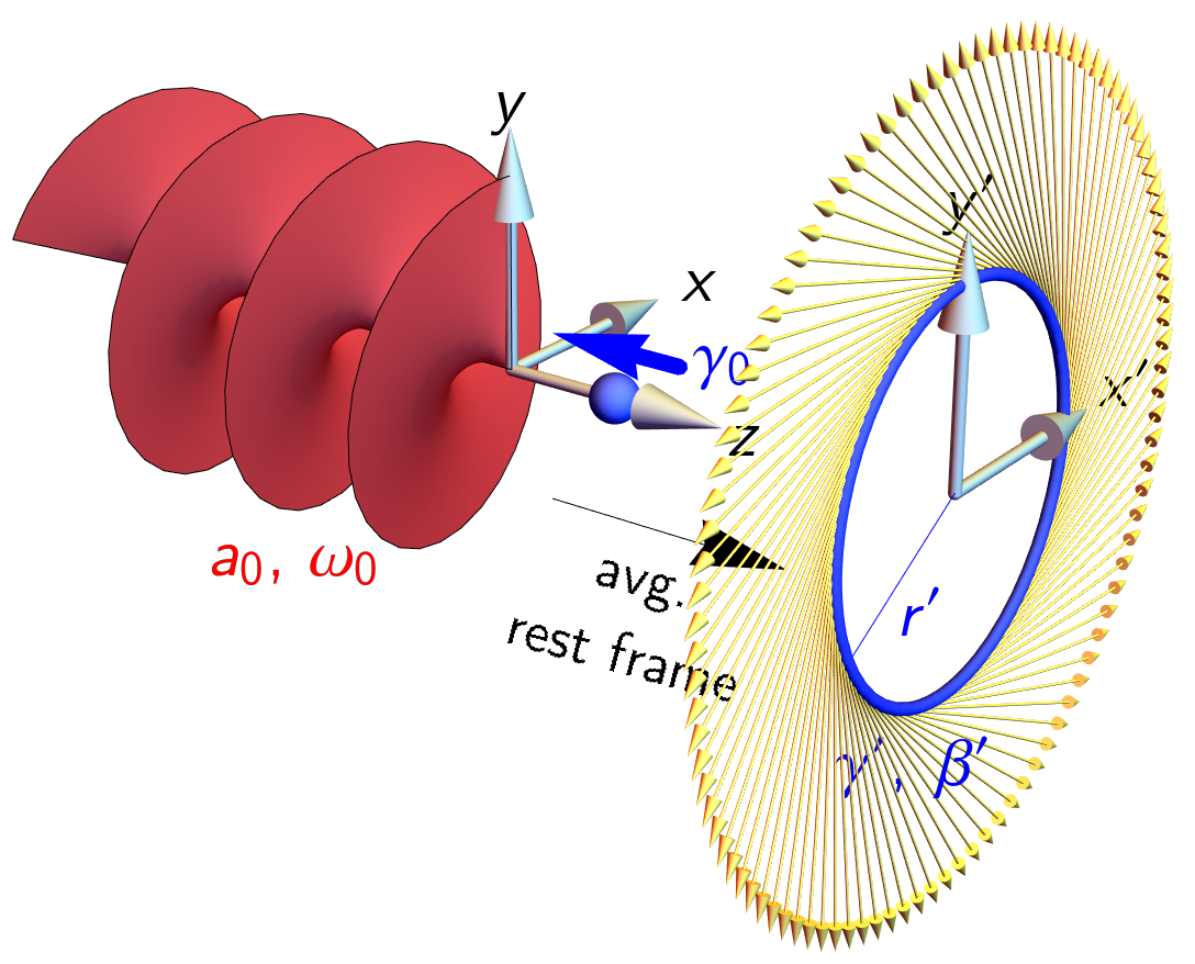
Figure 1: Interaction of an electron (initial Lorentz factor $\gamma_{0}$) and a circularly polarized electromagnetic wave (frequency $\omega_{0}$ and normalized amplitude $a_{0}$). In its average rest frame the electron is accelerated on a circular trajectory, with Lorentz factor $\gamma^{\prime}=(1+a_{0}^{2})^{1/2}$, velocity $\beta^{\prime}$ and radius $r^{\prime}$. The acceleration leads to the emission of synchrotron radiation, which has characteristic frequency $\omega^{\prime}\simeq\gamma^{\prime 3}/r^{\prime}$.

The electromagnetic field tensor for the wave is $eF_{\mu\nu}=ma_{0}\sum_{i}f_{i}^{\prime}(\phi)(k_{\mu}\varepsilon^{i}_{\nu}-k_{\nu}\varepsilon^{i}_{\mu})$, where $k$ is the wavevector, primes denote differentiation with respect to phase $\phi=k.x$, and the $\varepsilon_{1,2}$ are constant polarization vectors that satisfy $\varepsilon_{i}^{2}=-1$ and $k.\varepsilon_{i}=0$. Then the four-momentum of the electron $p$ may be written in terms of the potential $eA_{\mu}=ma_{0}\sum_{i}f_{i}(\phi)\varepsilon^{i}_{\mu}$:

$$p^{\mu}(\phi)=p_{0}^{\mu}+eA^{\mu}-\left(\frac{eA.p_{0}}{k.p_{0}}+\frac{e^{2}A^{2}}{2k.p_{0}}\right)k^{\mu}.$$ (1)

Translational symmetry guarantees that $k.p=k.p_{0}$. The electron trajectory $x^{\mu}(\phi)=\int(p^{\mu}/k.p)\,\mathrm{d}\phi$.

Let us say that the electron initially counterpropagates into a circularly polarized, monochromatic wave, with velocity $\beta_{0}$ and Lorentz factor $\gamma_{0}$. The electron is accelerated by the wave in the longitudinal direction, parallel to its wavevector, reaching a steady drift velocity of $\beta_{d}$. Transforming to the electron’s average rest frame (ARF), as shown in fig. 1, we find that the electron executes circular motion with Lorentz factor $\gamma^{\prime}=(1+a_{0}^{2})^{1/2}$, velocity $\beta^{\prime}=a_{0}(1+a_{0}^{2})^{-1/2}$ and radius $r^{\prime}=a_{0}/[\gamma_{0}(1+\beta_{0})\omega_{0}]$. That $\gamma^{\prime}$ is constant tells us that there is a phase shift of $\pi/2$ between the rotation of the velocity and electric field vectors $\mathbf{v}$ and $\mathbf{E}$, so $\mathbf{v}\cdot\mathbf{E}=0$ and the external field does no work on the charge.

The instantaneous acceleration of the charge is non-zero so the electron emits radiation while describing this orbit. We can use classical synchrotron theory (Sokolov and Ternov, 1968) to calculate the energy radiated in a single cycle $\mathcal{E}_{\text{rad}}$, as a fraction $f$ of the electron energy in the ARF $\gamma^{\prime}m$, with the result $f=\mathcal{E}_{\text{rad}}/(\gamma^{\prime}m)=4\pi R_{c}/3$. The magnitude of the radiation losses is controlled by the invariant classical radiation reaction parameter (Di Piazza et al., 2010)

$$R_{c} \equiv\frac{\alpha a_{0}^{2}\gamma_{0}(1+\beta_{0})\omega_{0}}{m}$$ (2)

$$\simeq 0.13\left(\frac{\mathcal{E}_{0}}{500~{}\text{MeV}}\right)\left(\frac{I_{0}}{10^{22}~{}\text{Wcm}^{-2}}\right)\left(\frac{\lambda}{{\mu\mathrm{m}}}\right).$$ (3)

Here $\mathcal{E}_{0}$ is the initial energy of the electron, $I_{0}=E_{0}^{2}$ the laser intensity and $\lambda=2\pi/\omega_{0}$ its wavelength.

If we define ‘significant’ radiation damping to be an energy loss of approximately 10% per period (Thomas et al., 2012), we find the threshold to be $R_{c}\gtrsim 0.024$, or $a_{0}\gamma_{0}^{1/2}\gtrsim 7\times 10^{2}$ for a laser with a wavelength of $0.8~{}{\mu\mathrm{m}}$. At this point the force on the electron due to radiative losses must be included in the equations of motion. We can see this directly by comparing the magnitudes of the radiation reaction and Lorentz forces. Estimating the former as $F_{\text{rad}}=\mathcal{E}_{\text{rad}}/(2\pi r^{\prime})$ and the Lorentz force as $F_{\text{ext}}=\gamma^{\prime}m/r^{\prime}$, we have that $F_{\text{rad}}/F_{\text{ext}}\simeq 2R_{c}/3$. For $R_{c}\gtrsim 1$ we enter the radiation-dominated regime (Bulanov et al., 2004; Koga et al., 2005; Hadad et al., 2010).

We will discuss how the recoil due to radiation emission is included in classical electrodynamics in section II.1. Before doing so, let us also consider the spectral characteristics of the radiation emitted by the accelerated electron. In principle the periodicity of the motion, and its infinite duration, means that the frequency spectrum is made up of harmonics of the ARF cyclotron frequency. However, recall that at large $\gamma^{\prime}\simeq a_{0}$, relativistic beaming means that most of the radiation is emitted in the forward direction into a cone with half-angle $1/\gamma^{\prime}$. The length of the overlap between the electron trajectory and this cone defines the formation length $l_{f}$, which is the characteristic distance over which radiation is emitted (Ter-Mikaelian, 1953; Klein, 1999). A straightforward geometrical calculation gives the ratio between $l_{f}$ and the circumference of the orbit $C=2\pi r^{\prime}$

$$\frac{l_{f}}{C}\simeq\frac{1}{2\pi a_{0}}.$$ (4)

The invariance of $a_{0}$ suggests we could have reached this result in a covariant way; indeed, a full determination of the size of the phase interval that contributes to emission gives the same result, even quantum mechanically (Ritus, 1985).

The smallness of the formation zone means that the spectrum is broadband, with frequency components up to a characteristic value $\omega^{\prime}\simeq\gamma^{\prime 3}/r^{\prime}$. Comparing this characteristic frequency to the cyclotron frequency (in the average rest frame) $\omega_{c}=1/r^{\prime}$ gives us a measure of the classical nonlinearity:

$$\frac{\omega^{\prime}}{\omega_{c}}\simeq a_{0}^{3}.$$ (5)

At $a_{0}\gg 1$, the radiation is made up of very high harmonics and is therefore well-separated from the background. The ratio between the frequency $\omega^{\prime}$ and the electron energy in the ARF $\chi=\omega^{\prime}/(\gamma^{\prime}m)$ is another useful invariant parameter

$$\chi \equiv\frac{a_{0}\gamma_{0}(1+\beta_{0})\omega_{0}}{m}$$ (6)

$$\simeq 0.29\left(\frac{\mathcal{E}_{0}}{500~{}\text{MeV}}\right)\left(\frac{I_{0}}{10^{22}~{}\text{Wcm}^{-2}}\right)^{1/2}.$$ (7)

Restoring factors of $\hbar$ and $c$ we can show that $\chi\propto\hbar$, unlike $R_{c}$. It therefore parametrizes the importance of quantum effects on radiation reaction (Ritus, 1985; Erber, 1966), as can be seen by the fact that if $\chi\sim 1$, an individual photon of the radiation can carry off a substantial fraction of the electron’s energy. By setting $\gamma_{0}=1$ in eq. 6, we can show that $\chi$ is equal to the ratio of the electric field in the instantaneous rest frame of the electron to the so-called critical field of QED (Sauter, 1931; Heisenberg and Euler, 1936)

$$E_{\text{cr}}\equiv\frac{m^{2}}{e}=1.326\times 10^{18}~{}\text{Vm}^{-1},$$ (8)

which famously marks the threshold for nonperturbative electron-positron pair creation from the vacuum (Schwinger, 1951).

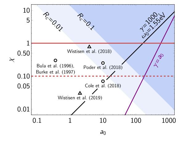
Figure 2: The importance, and type, of radiation reaction effects can be parametrized by $a_{0}$, the normalized intensity of the laser field or classical nonlinearity parameter, and $\chi$, the quantum nonlinearity parameter. Classical radiation damping becomes strong when $R_{c}=\alpha a_{0}\chi>0.01$ (light blue) and dominates when $R_{c}>0.1$ (darker blue). Quantum corrections to the spectrum become necessary when $\chi>0.1$. Electron-positron pair creation and QED cascades are important for $\chi>1$. Experiments that have explored quantum effects with intense lasers are shown by open circles (Bula et al., 1996; Burke et al., 1997; Cole et al., 2018; Poder et al., 2018). Two recent experiments with lepton beams and aligned crystals are shown by triangles (Wistisen et al., 2018, 2019); here the perpendicular component of the lepton momentum $p_{\perp}$ is used to define an equivalent classical nonlinearity parameter $a_{0}\simeq p_{\perp}/m$.

The two parameters $R_{c}$ and $\chi$ allow us to characterize the importance of classical and quantum radiation reaction respectively. We show these as functions of $a_{0}$ and $\chi$, the classical and quantum nonlinearity parameters, in fig. 2. It is evident that, as $a_{0}$ increases, it requires less and less electron energy to enter the radiation-dominated regime. Indeed, if the acceleration is provided entirely by the laser so that $\gamma\simeq a_{0}$, radiation reaction becomes dominant at about the same $a_{0}$ that quantum effects become important, assuming that $\omega_{0}$ corresponds to a wavelength of $0.8~{}{\mu\mathrm{m}}$. However, for $a_{0}\lesssim 50$ as is accessible with existing lasers (Bahk et al., 2004; Sung et al., 2017; Kiriyama et al., 2018), it is not possible to probe radiation reaction via direct illumination of a plasma. Instead, the experiments illustrated in fig. 2 have used pre-accelerated electrons to explore the strong-field regime, thereby boosting both $R_{c}$ and $\chi$. (Note that, as $R_{c}$ is defined on a per-cycle basis, it would be possible for classical radiation reaction effects to be large in long laser pulses while remaining below the threshold for quantum effects.) The next generation of laser facilities will reach $a_{0}$ in excess of 100, perhaps even $1000$ (Papadopoulos et al., 2016; Weber et al., 2017; Gales et al., 2018). The plasma dynamics explored in such experiments will be strongly affected by radiation reaction and quantum effects.

II Theory of radiation reaction

II.1 Classical radiation reaction

In classical electrodynamics, radiation reaction is the response of a charged particle to the field of its own radiation (Lorentz, 1904; Abraham, 1905). The first equation of motion to include both the external and self-induced electromagnetic forces in a manifestly covariant and self-consistent way was obtained by Dirac (1938). This solution starts from the coupled Maxwell’s and Lorentz equations and features a mass renormalization that is needed to eliminate divergences associated with a point-like charge (Erber, 1961; Teitelboim, 1971). The result is generally referred to as the Lorentz-Abraham-Dirac (LAD) equation. For an electron with four-velocity $u$, charge $-e$ and mass $m$ it reads

$$\frac{\mathrm{d}u^{\mu}}{\mathrm{d}\tau}=-\frac{e}{m}F^{\mu\nu}u_{\nu}+\frac{e^{2}}{6\pi m}\left(\frac{\mathrm{d}^{2}u^{\mu}}{\mathrm{d}\tau^{2}}+u^{\mu}\frac{\mathrm{d}u_{\nu}}{\mathrm{d}\tau}\frac{\mathrm{d}u^{\nu}}{\mathrm{d}\tau}\right)$$ (9)

where $\tau$ is the proper time. Here $F_{\mu\nu}$ is the field tensor for the externally applied electromagnetic field, so it is the second term that accounts for the self-force. Although the LAD equation is an exact solution of the Maxwell-Lorentz system, using it directly turns out to be problematic. The momentum derivative $\frac{\mathrm{d}^{2}u^{\mu}}{\mathrm{d}\tau^{2}}$ in the RR term leads to so-called runaway solutions, in which the electron energy increases exponentially in the absence of external fields, and to pre-acceleration, in which the momentum changes in advance of a change in the applied field (Spohn, 2004; Yaghjian, 2006; Rohrlich, 2007). These issues have prompted searches for alternative classical theories of radiation reaction (Mo and Papas, 1971; Bonnor, 1974; Eliezer, 1948; Ford and O’Connell, 1991; Sokolov, 2009) that have more satisfactory properties (see the review by Burton and Noble (2014) for details).

The most widely used classical theory is that proposed by Landau and Lifshitz (1987). They realized that if the second (RR) term in eq. 9 were much smaller than the first in the instantaneous rest frame of the charge, it would be possible to reduce the order of the LAD equation by substituting $\frac{\mathrm{d}u}{\mathrm{d}\tau}\to\frac{e}{m}F^{\mu\nu}u_{\nu}$ in the RR term. The result, called the Landau-Lifshitz equation, is first-order in the electron momentum and free from the pathological solutions of the LAD equation (Burton and Noble, 2014):

$$\frac{\mathrm{d}u^{\mu}}{\mathrm{d}\tau}=-\frac{e}{m}F^{\mu\nu}u_{\nu}+\frac{e^{4}}{6\pi m}\left[-\frac{m}{e}(\partial_{\alpha}F^{\mu\nu})u_{\nu}u^{\alpha}\right.\\ \left.+F^{\mu\nu}F_{\nu\alpha}u^{\alpha}+(F^{\nu\alpha}u_{\alpha})^{2}u^{\mu}\right].$$ (10)

The following two conditions for the characteristic length scale $L$ over which the field varies and its magnitude $E$ must be fulfilled in the instantaneous rest frame for the order reduction procedure to be valid: $L\gg\lambda_{C}$ and $E\ll E_{\text{cr}}/\alpha$, where $\lambda_{C}=1/m$ is the Compton length. Note that both of these are automatically fulfilled in the realm of classical electrodynamics (Di Piazza et al., 2012), as quantum effects can only be neglected when $L\gg\lambda_{C}$ and $E\ll E_{\text{cr}}$. The former condition ensures that the electron wavefunction is well-localized and the latter means recoil at the level of the individual photon is negligible (Di Piazza et al., 2012). One reason to favour the Landau-Lifshitz equation is that all physical solutions of the LAD equation are solutions of the Landau-Lifshitz equation (Spohn, 2000).

Once the trajectories are determined, the self-consistent radiation is obtained from the Liénard-Wiechert potentials, which give the electric and magnetic fields of a charge in arbitrary motion (Jackson, 1999). The spectral intensity of the radiation from an ensemble of $N_{e}$ electrons, the energy radiated per unit frequency $\omega$ and solid angle $\Omega$, is given in the far field by

$$\frac{\mathrm{d}^{2}\mathcal{E}}{\mathrm{d}\omega\mathrm{d}\Omega}=\frac{\alpha\omega^{2}}{4\pi^{2}}\left|\sum_{k=1}^{N_{e}}\int_{-\infty}^{\infty}\mathbf{n}\times(\mathbf{n}\times\mathbf{v}_{k})e^{i\omega(t-\mathbf{n}\cdot\mathbf{r}_{k})}\,\mathrm{d}t\right|^{2}$$ (11)

where $\mathbf{n}$ the observation direction, and $\mathbf{r}_{k}$ and $\mathbf{v}_{k}$ are the position and velocity of the $k$th particle at time $t$ (Jackson, 1999).

II.1.1 In plane electromagnetic waves

Among the other useful properties of eq. 10 is that it can be solved exactly if the external field is a plane electromagnetic wave (Di Piazza, 2008). Taking this field to be $eF_{\mu\nu}=ma_{0}\sum_{i}f_{i}^{\prime}(\phi)(k_{\mu}\varepsilon^{i}_{\nu}-k_{\nu}\varepsilon^{i}_{\mu})$, using the same definitions as in section I, eq. 10 is most conveniently expressed in terms of the lightfront momentum $u^{-}\equiv k.p/(m\omega_{0})$, scaled perpendicular momenta $\tilde{u}_{x,y}\equiv u_{x,y}/u^{-}$, and phase $\phi$:

$$\frac{\mathrm{d}u^{-}}{\mathrm{d}\phi}=-\frac{2\alpha a_{0}^{2}\omega_{0}}{3m}[f^{\prime}_{1}(\phi)^{2}+f^{\prime}_{2}(\phi)^{2}]{u^{-}}^{2},$$ (12)

and

$$\frac{\mathrm{d}\tilde{u}_{i}}{\mathrm{d}\phi}=\frac{a_{0}f_{i}^{\prime}(\phi)}{u^{-}}+\frac{2\alpha a_{0}\omega_{0}f_{i}^{\prime\prime}(\phi)}{3m}.$$ (13)

The remaining component $u^{+}$ is determined by the mass-shell condition $u^{-}u^{+}-u_{x}^{2}-u_{y}^{2}=1$ and the position by integration of $\omega_{0}x^{\mu}(\phi)=\int_{-\infty}^{\phi}(u^{\mu}/u^{-})\,\mathrm{d}\phi$. Equation 12 admits the solution

$$u^{-}=\frac{u^{-}_{0}}{1+\frac{2}{3}R_{c}I(\phi)},$$ (14)

where $u^{-}_{0}$ is the initial lightfront momentum, the classical radiation reaction parameter $R_{c}=a_{0}^{2}u^{-}_{0}\omega_{0}/m$ as in eq. 2, and $I(\phi)=\int_{-\infty}^{\phi}[f_{1}^{\prime}(\psi)^{2}+f_{2}^{\prime}(\psi)^{2}]\,\mathrm{d}\psi$. The choice of notation here reflects the fact that $f^{\prime}(\phi)$ is proportional to the electric field and so $I(\phi)$ is like an integrated energy flux. We use eq. 14 to solve eq. 13, obtaining $\tilde{u}_{i}(\phi)$ and then

$$u_{i}=\frac{1}{1+\frac{2}{3}R_{c}I(\phi)}\left[u_{i,0}+a_{0}f_{i}(\phi)+\frac{2R_{c}}{3}H(\phi)+\frac{2R_{c}}{3a_{0}}f_{i}^{\prime}(\phi)\right],$$ (15)

where $u_{i,0}$ is the initial value of the perpendicular momentum component $i$ and $H_{i}(\phi)=\int_{-\infty}^{\phi}\!f_{i}^{\prime}(\psi)I(\psi)\,\mathrm{d}\psi$. The electron trajectory in the absence of radiation reaction is obtained by setting $\alpha=0$, in which case we recover eq. 1 as expected. Note that the lightfront momentum $u^{-}$ is no longer conserved, once radiation reaction is taken into account (Harvey et al., 2011).

In section I we estimated that the electron would radiate in a single cycle a fraction $4\pi R_{c}/3$ of its total energy. Using our analytical result eq. 14 and assuming $\gamma\gg 1$ so that $u^{-}\simeq 2\gamma$, we can show this fraction is actually $\mathcal{E}_{\text{rad}}/(\gamma_{0}m)=(4\pi R_{c}/3)/(1+4\pi R_{c}/3)$. Here the denominator represents radiation-reaction corrections to the energy loss, guaranteeing that $\mathcal{E}_{\text{rad}}/(\gamma_{0}m)<1$. With these corrections, the energy emitted, according to the Larmor formula, is equal to the energy lost, according to the Landau-Lifshitz equation (see Appendix A of Di Piazza (2018) for a direct calculation of momentum conservation).

The emission spectrum eq. 11 may also be expressed in terms of an integral over phase. The number of photons scattered per unit (scaled) frequency $s=\omega/\omega_{0}$ and solid angle is (Esarey et al., 1993; Hartemann et al., 2010)

$$\frac{\mathrm{d}^{2}N_{\gamma}}{\mathrm{d}s\mathrm{d}\Omega}=\frac{\alpha s}{4\pi^{2}}\left|\sum_{k=1}^{N_{e}}\int_{-\infty}^{\infty}\!\frac{\varepsilon^{\prime}.u_{k}\exp(-isn.\xi_{k})}{(u^{-}_{k})^{2}}\,\mathrm{d}\phi\right|^{2}$$ (16)

where the scaled four-position $\xi\equiv\omega_{0}x$, and $\varepsilon^{\prime}$ and $n$ are the four-polarization and propagation direction of the scattered photon. Given these relations and the analytically determined trajectory, we can numerically evaluate the number of photons scattered to given frequency and polar angle by integrating eq. 16, summed over polarizations, over all azimuthal angles $0\leq\varphi<2\pi$.

II.2 Quantum corrections: suppression and stochasticity

We showed in fig. 2 that in many scenarios of interest, reaching the regime where radiation reaction becomes important automatically makes quantum effects important as well. This raises the question: what is the quantum picture of radiation reaction? Let us revisit the example we studied classically in section I, that of an electron emitting radiation under acceleration by a strong electromagnetic wave. One might instinctively liken this scenario to inverse Compton scattering, as energy and momentum are automatically conserved when the electron absorbs a photon (or photons) from the plane wave and emits another, higher energy photon. However, the recoil is proportional to $\hbar$ and vanishes in the classical limit; we would then recover Thomson scattering rather than radiation reaction.

The solution is that, in the regime $a_{0}\gg 1$ and $\chi\lesssim 1$, quantum radiation reaction can be identified with the recoil on the electron due its emission of multiple, incoherent photons (Di Piazza et al., 2010). These conditions express the following: $a_{0}\gg 1$ means that the formation length is much smaller than the wavelength of the external field, by eq. 4, so the coherent contribution is suppressed; and $\chi\lesssim 1$ means pair creation can be neglected. The latter is important because QED is inherently a many-body theory and it is possible for the final state to contain many more electrons than the initial state. As the number of photons $N_{\gamma}\propto\alpha\propto 1/\hbar$ and the momentum change of the electron $\propto\hbar$ for each photon, we have that the total momentum change $\propto\hbar^{0}$ and therefore a classical limit exists (Di Piazza et al., 2012). This suggests that one way to determine the ‘correct’ theory of classical radiation reaction is to start with a QED result and take the limit $\hbar\to 0$. This has been accomplished for both the momentum change (Krivitski and Tsytovich, 1991; Ilderton and Torgrimsson, 2013a) and the position (Ilderton and Torgrimsson, 2013b). In particular, Ilderton and Torgrimsson (2013b) were able to show that, to first order in $\alpha$, only the LAD, Landau-Lifshitz and Eliezer-Ford-O’Connell formulations of radiation reaction were consistent with QED.

In both the classical and quantum regimes, the force of radiation reaction is directed antiparallel to the electron’s instantaneous momentum, and its magnitude depends on the parameter $\chi$. We defined this earlier for the particular case of an electron in an electromagnetic wave [see eq. 6]. In a general electromagnetic field $F_{\mu\nu}$,

$$\chi=\frac{\sqrt{-(F_{\mu\nu}p^{\nu})^{2}}}{mE_{\text{cr}}}=\frac{\gamma}{E_{\text{cr}}}\sqrt{(\mathbf{E}+\mathbf{v}\times\mathbf{B})^{2}-(\mathbf{v}\cdot\mathbf{E})^{2}},$$ (17)

where $p=\gamma m(1,\mathbf{v})$ is the electron four-momentum. $\chi$ depends on the instantaneous transverse acceleration induced by the external field: in a plane EM wave, where $\mathbf{E}$ and $\mathbf{B}$ have the same magnitude and are perpendicular to each other, $\chi=\gamma\left|\mathbf{E}\right|(1-\cos\theta)/E_{\text{cr}}$, where $\theta$ is the angle between the electron momentum and the laser wavevector, and it is therefore largest in counterpropagation. A curious consequence of eq. 17 is the existence of a radiation-free direction: no matter the configuration of $\mathbf{E}$ and $\mathbf{B}$, there exists a particular $\mathbf{v}$ that makes $\chi$ vanish (Gonoskov and Marklund, 2018). Electrons in extremely strong fields tend to align themselves with this direction, any transverse momentum they have being rapidly radiated away (Gonoskov and Marklund, 2018). As this direction is determined purely by the fields, the self-consistent evolutions of particles and fields is determined by hydrodynamic equations (Samsonov et al., 2018).

The larger the value of $\chi$, the greater the differences between the quantum and classical predictions of radiation emission. Classically there is no upper limit on the frequency spectrum, whereas in the quantum theory there appears a cutoff that guarantees $\omega<\gamma m$. Besides this cutoff, spin-flip transitions enhance the spectrum at high energy (Uggerhøj, 2005). Let us work in the synchrotron limit, wherein the field may be considered constant over the formation length (i.e. $l_{f}\ll\lambda$, using eq. 4). The classical emission spectrum, the energy radiated per unit frequency $\omega=x\gamma m$ and time by an electron with quantum parameter $\chi$ and Lorentz factor $\gamma$, is

$$\frac{\mathrm{d}\mathcal{P}_{\text{cl}}}{\mathrm{d}\omega} =\frac{\alpha\omega}{\sqrt{3}\pi\gamma^{2}}\left[2K_{2/3}(\xi)-\int_{\xi}^{\infty}\!K_{1/3}(y)\,\mathrm{d}y\right], \xi =\frac{2x}{3\chi}.$$ (18)

Two quantum corrections emerge when $\chi$ is no longer much smaller than one: the non-negligible recoil of an individual photon means that the spectrum has a cutoff at $x=1$; and the spin contribution to the radiation must be included. The former can be included directly by modifying $\xi=2x/(3\chi)\to 2x/[3\chi(1-x)]$ in eq. 18, which yields the spectrum of a spinless electron (shown in orange in fig. 3). A neat exposition of this simple substitution is given by Lindhard (1991) in terms of the correspondence principle (see also Sørensen (1996)). Then when the spin contribution is added, we obtain the full QED result (Erber, 1966; Ritus, 1985; Baier et al., 1998)

$$\frac{\mathrm{d}\mathcal{P}_{\text{q}}}{\mathrm{d}\omega} =\frac{\alpha\omega}{\sqrt{3}\pi\gamma^{2}}\left[\left(1-x+\frac{1}{1-x}\right)K_{2/3}(\xi)-\int_{\xi}^{\infty}\!K_{1/3}(y)\,\mathrm{d}y\right], \xi =\frac{2x}{3\chi(1-x)},$$ (19)

where we quote the spin-averaged and polarization-summed result. This is shown in blue in fig. 3. The number spectrum $\frac{\mathrm{d}N_{\gamma}}{\mathrm{d}\omega}=\omega^{-1}\frac{\mathrm{d}\mathcal{P}_{\text{q}}}{\mathrm{d}\omega}(\chi,\gamma)$ has an integrable singularity $\propto\omega^{-2/3}$ in the limit $\omega\to 0$. The total number of photons $N_{\gamma}=\int\frac{\mathrm{d}N_{\gamma}}{\mathrm{d}\omega}\mathrm{d}\omega$ is finite.

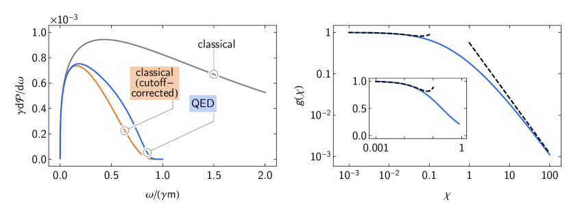
Figure 3: (left) Quantum corrections to the emission spectrum $\mathrm{d}\mathcal{P}/\mathrm{d}\omega$ at $\chi=1$: the classical [eq. 18] and quantum-corrected spectra [eq. 19]. (right) These corrections cause the total radiated power to be reduced by a factor $g(\chi)$: the full result (blue) and limiting expressions (black, dashed).

The combined effect of these corrections is to reduce the instantaneous power radiated by an electron. This reduction is quantified by the factor $g(\chi)=\mathcal{P}_{\text{q}}/\mathcal{P}_{\text{cl}}$, which takes the form (Erber, 1966; Sokolov and Ternov, 1968)

$$g(\chi) =\frac{9\sqrt{3}}{8\pi}\int_{0}^{\infty}\left[\frac{2u^{2}K_{5/3}(u)}{(2+3\chi u)^{2}}+\frac{36\chi^{2}u^{3}K_{2/3}(u)}{(2+3\chi u)^{4}}\right]\mathrm{d}u$$ (20)

$$=\begin{cases}1-\frac{55\sqrt{3}}{16}\chi+48\chi^{2}&\chi\ll 1\\ \frac{16\Gamma(2/3)}{3^{1/3}27}\chi^{-4/3}&\chi\gg 1\end{cases}$$ (21)

where $K$ is a modified Bessel function of the second kind and $\Gamma(2/3)\simeq 1.354$. The limiting expressions given in eq. 21 are within 5% of the full result for $\chi<0.05$ and $\chi>200$ respectively. A simple analytical approximation to eq. 20 that is accurate to 2% for arbitrary $\chi$ is $g(\chi)\simeq[1+4.8(1+\chi)\ln(1+1.7\chi)+2.44\chi^{2}]^{-2/3}$ (Baier et al., 1998). The changes to the classical radiation spectrum and the magnitude of $g(\chi)$ are shown in fig. 3. Note that the total power $\mathcal{P}_{\text{q}}=2\alpha m^{2}\chi^{2}g(\chi)/3$ always increases with increasing $\chi$. $g(\chi)$ is sometimes referred to as the ‘Gaunt factor’ (Ridgers et al., 2017), as it is a multiplicative (quantum) correction to a classical result, first derived in the context of absorption (Gaunt, 1930).

Figure 3 shows that the radiated power at $\chi\sim 1$ is less than $20\%$ of its classically predicted value. While this suppression does have a marked effect on the particle dynamics, it is not the only quantum effect. As is discussed in section I, $\chi$ is the ratio between the energies of the typical photon and the emitting electron. When this approaches unity, even a single emission can carry off a large fraction of the electron energy, and the concept of a continuously radiating particle breaks down. Instead, electrons lose energy probabilistically, in discrete portions. The importance of this discreteness may be estimated by comparing the typical time interval between emissions, $\Delta t=\langle\omega\rangle/\mathcal{P}$, with the timescale of the laser field $1/\omega_{0}$ (Gonoskov et al., 2015). Equation 19 yields for the average photon energy $\langle\omega\rangle\simeq 0.429\,\chi\gamma m$ for $\chi\ll 1$ and $0.25\,\gamma m$ for $\chi\gg 1$; the radiated power $\mathcal{P}=2\alpha m^{2}\chi^{2}g(\chi)/3$. We find

$$\omega_{0}\Delta t\simeq\begin{cases}44\,a_{0}^{-1}&\chi\ll 1\\ 58\,[\gamma\omega_{0}/(a_{0}m)]^{1/3}&\chi\gg 1\end{cases}.$$ (22)

We expect stochastic effects to be at their most significant when $\omega_{0}\Delta t\gtrsim 1$, which implies that the total number of emissions in an interaction is relatively small but $\chi$ is large.

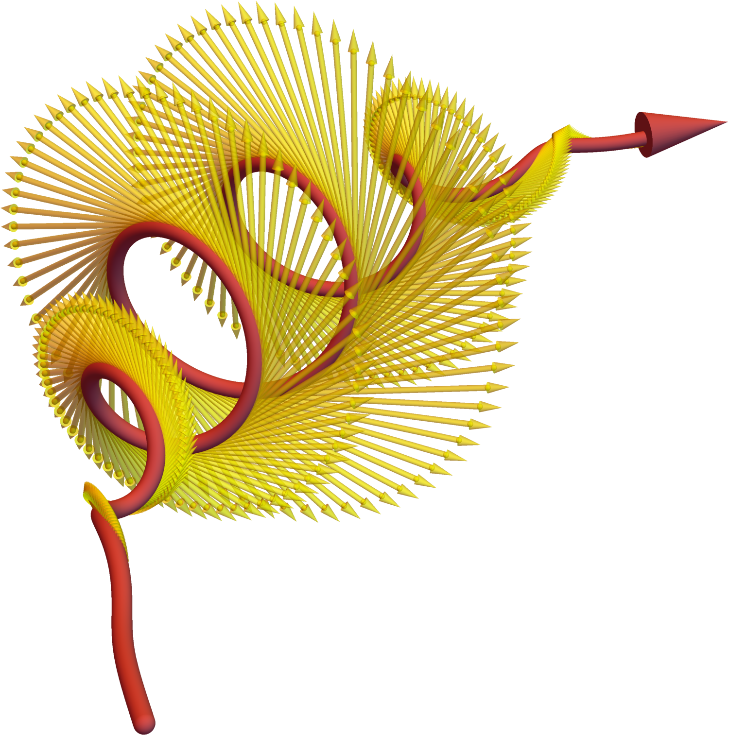
Figure 4: In the classical picture, radiation reaction is a continuous drag force that arises from the emission of very many photons that individually have vanishingly low energies (left). In the quantum regime, however, the electrons emits a finite number of photons, any or all of which can exert a significant recoil on the electron. The probabilistic nature of emission leads to radically altered electron dynamics, with implications for laser-matter interactions beyond the current intensity frontier. From Blackburn (2015).

A description of how stochastic energy losses can be modelled follows in section III.2. For now, it suffices to interpret eq. 19 as the (energy-weighted) probability distribution of the photons emitted at a particular instant of time. Even though two electrons may have the same $\chi$ and $\gamma$, they can emit photons of different energies (or none at all) and thereby experience different recoils. Contrast this with the classical picture, in which the continuous energy loss is driven by the emission of many photons that individually have vanishingly small energies (see fig. 4).

Consider, for example, the interaction of a beam of electrons with a plane electromagnetic wave, where the Lorentz factors of the electrons are distributed $\gamma\sim\frac{\mathrm{d}N_{e}}{\mathrm{d}\gamma}$. The distribution is characterized by a mean $\mu\equiv\langle\gamma\rangle$ and variance $\sigma^{2}\equiv\langle\gamma^{2}\rangle-\mu^{2}$. Under classical radiation reaction, higher energy electrons are guaranteed to radiate more than their lower energy counterparts ($\mathcal{P}\propto\gamma^{2}$), with the result that both the mean and the variance of $\gamma$ decrease over the course of the interaction (Neitz and Di Piazza, 2013). This is still the case if the radiated power is reduced by the Gaunt factor $g(\chi)$, i.e. a ‘modified classical’ model is assumed (see section III.1), because radiation losses remain deterministic (Yoffe et al., 2015).

Under quantum radiation reaction, radiation losses are inherently probabilistic. While $\mu$ will still decrease (more energetic electrons radiate more energy on average), the width of the distribution $\sigma^{2}$ can actually grow (Neitz and Di Piazza, 2013; Vranic et al., 2016a). Ridgers et al. (2017) derive the following equations for the temporal evolution of these quantities, under quantum radiation reaction:

$$\frac{\mathrm{d}\mu}{\mathrm{d}t} =-\frac{2\alpha m}{3}\langle\chi^{2}g(\chi)\rangle$$ (23)

$$\frac{\mathrm{d}\sigma^{2}}{\mathrm{d}t} =-\frac{4\alpha m}{3}\langle(\gamma-\mu)\chi^{2}g(\chi)\rangle+\frac{55\alpha m}{24\sqrt{3}}\langle\gamma\chi^{3}g_{2}(\chi)\rangle,$$ (24)

where $\langle\cdots\rangle$ denotes the population average and $g_{2}(\chi)=\int\!\chi\,\mathrm{d}\mathcal{P}_{\text{q}}/\int\!\chi\,\mathrm{d}\mathcal{P}_{\text{cl}}$ is the second moment of the emission spectrum. Only the first term of eq. 24 is non-zero in the classical limit, and it is guaranteed to be negative. The second term represents stochastic effects and is always positive. Broadly speaking, the latter is dominant if $\chi$ is large, the interaction is short, or the initial variance is small (Ridgers et al., 2017; Niel et al., 2018). The evolution of higher order moments, such as the skewness of the distribution, are considered in Niel et al. (2018).

A distinct consequence of stochasticity is straggling (Shen and White, 1972), where an electron that radiates less (or no) energy than expected enters regions of phase space that would otherwise be forbidden. Unlike stochastic broadening, which can occur in a static, homogeneous electromagnetic field, straggling requires the field to have some non-trivial spatiotemporal structure. If an unusually long interval passes between emissions, an electron may be accelerated to a higher energy or sample the fields at locations other than those along the classical trajectory (Duclous et al., 2011). In a laser pulse with a temporal envelope, for example, electrons that traverse the intensity ramp without radiating reach larger values of $\chi$ than would be possible under continuous radiation reaction; this enhances high-energy photon production and electron-positron pair creation (Blackburn et al., 2014). If the laser duration is short enough, it is probable that the electron passes through the pulse without emitting at all, in so-called quenching of radiation losses (Harvey et al., 2017).

The quantum effects we have discussed in this section emerge, in principle, from analytical results including the emission spectrum [eq. 19]. While further analytical progress can be made in the quantum regime, using the theory of strong-field QED (see section III.2), modelling more realistic laser–electron-beam or laser-plasma interactions generally requires numerical simulations. Much effort has been devoted to the development, improvement, benchmarking and deployment of such simulation tools over the last few years. In the following section we review these continuing developments.

III Numerical modelling and simulations

III.1 Classical regime

A natural starting point is the modelling of classical radiation reaction effects. In the absence of quantum corrections, we have all the ingredients we need to formulate a self-consistent picture of radiation emission and radiation reaction. We showed in section I how using only the Lorentz force to determine the charge’s motion and therefore its emission led to an inconsistency in energy balance. This is remedied by using either eq. 9 or eq. 10 as the equation of motion, in which case the energy carried away in radiation matches that which is lost by the electron.

Implementations of classical radiation reaction in plasma simulation codes have largely favoured the Landau-Lifshitz equation (or a high-energy approximation thereto), as it is first-order in the momentum and the additional computational cost is not large (Tamburini et al., 2010; Harvey et al., 2011; Green and Harvey, 2015; Vranic et al., 2016b). These codes have not only been used to study radiation reaction effects in laser-plasma interactions (Chen et al., 2011; Nakamura et al., 2012; Vranic et al., 2014; Tamburini et al., 2014; Yoffe et al., 2015; Liseykina et al., 2016), but also whether there are observable differences between models of the same (Bulanov et al., 2011b; Kravets et al., 2013). The radiation reaction force proposed by Sokolov (2009) has also been implemented in some codes (Sokolov et al., 2011; Capdessus et al., 2012), but note that it is not consistent with the classical limit of QED (Ilderton and Torgrimsson, 2013b). It is also possible to solve the LAD equation numerically via integration backward in time (Koga, 2004).

Given data on the trajectories of an ensemble of electrons (usually a subset of the all electrons in the simulations), eq. 11 can be used to obtain the far-field spectrum in a simulation where classical radiation reaction effects are included (Thomas et al., 2012; Schlegel and Tikhonchuk, 2012; Martins et al., 2016). Equation 11 is valid across the full range of $\omega$ (pace the quantum cutoff at $\omega=\gamma m$), including the low-frequency region of the spectrum where collective effects are important: $\omega<n_{e}^{1/3}$, where $n_{e}$ is the electron number density. This region does not, however, contribute very much to radiation reaction; this is dominated by photons near the synchrotron critical energy $\omega_{c}\gg n_{e}^{1/3}$. Thus the spectrum can be divided into coherent and incoherent parts, that are well separated in terms of their energy (Gonoskov et al., 2015). In the latter region, the order of the summation and integration in eq. 11 can be exchanged, and the total spectrum determined by summing over the single-particle spectra.

In a particle-in-cell code for example, the electromagnetic field is defined on a grid of discrete points and advanced self-consistently using currents that are deposited onto the same grid (Dawson, 1983). Defining the grid spacing to be $\Delta$, this scheme will directly resolve electromagnetic radiation that has a frequency less than the Nyquist frequency $\pi/\Delta$. Given appropriately high resolution, this accounts for the coherent radiation generated by the collective dynamics of the ensemble of particles. The recoil arising from higher frequency components, which cannot be resolved on the grid, and in any case as a self-interaction is neglected, is accounted for by the radiation reaction force.

Further simplification is possible if the interference of emission from different parts of the trajectory is negligible. As indicated in section I, at high intensity $a_{0}\gg 1$, the formation length of the radiation is much smaller than the timescale of the external field (see eq. 4). This being the case, rather than using eq. 11, we may integrate the local emission spectrum eq. 18 over the particle trajectory, assuming that, at high $\gamma$, the radiation is emitted predominantly in direction parallel to the electron’s instantaneous velocity (Esarey et al., 1993; Reville and Kirk, 2010; Wallin et al., 2015). The approach is naturally extended to account for quantum effects, by substituting for the classical synchrotron spectrum eq. 18 the equivalent result in QED, eq. 19.

One consequence of doing so is that the radiated power is reduced by the factor $g(\chi)$, given in eq. 20. This should be reflected in a reduction in the magnitude of the radiation-reaction force. Consequently, a straightforward, phenomenological way to model quantum radiation reaction is to use a version of eq. 10 where the second term is scaled by $g(\chi)$. This ‘modified classical’ model has been used in studies of laser–electron-beam (Thomas et al., 2012; Blackburn et al., 2014; Yoffe et al., 2015) and laser-plasma interactions (Kirk et al., 2009; Zhang et al., 2015) as a basis of comparison with a fully stochastic model (shortly to be introduced), as well as in experimental data analysis (Wistisen et al., 2018; Poder et al., 2018). It has been shown that this approach yields the correct equation of motion for the average energy of an ensemble of electrons in the quantum regime (Ridgers et al., 2017; Niel et al., 2018). It is, however, deterministic, and therefore neglects the stochastic effects we discussed in section II.2.

III.2 Quantum regime: the ‘semiclassical’ approach

In section II.2 we discussed how ‘quantum radiation reaction’ could be identified with the recoil arising from multiple, incoherent emission of photons. Indeed, if $\chi\gtrsim 1$, any or all of these photons can exert a significant momentum change individually. Figure 2 tells us that we generally require $a_{0}\gg 1$ to enter the quantum radiation reaction regime with lasers, which necessitates a nonperturbative approach to the theory. This is provided by strong-field QED, which separates the electromagnetic field into a fixed background, treated exactly, and a fluctuating part, treated perturbatively (Furry, 1951); see the reviews by Ritus (1985); Di Piazza et al. (2012); Heinzl (2012) or a tutorial overview by Seipt (2017) which discusses photon emission in particular.

Although it is the most general and accurate approach, strong-field QED is seldom used to model experimentally relevant configurations of laser-electron interaction (Blackburn et al., 2018). In a scattering-matrix calculation, the object is to obtain the probability of transition between asymptotic free states; as such, complete information about the spatiotemporal structure of the background field is required. Analytical results have only been obtained in field configurations that possess high symmetry (Heinzl and Ilderton, 2017), e.g. plane EM waves (Ritus, 1985) or static magnetic fields (Erber, 1966). The assumption that the background is fixed also means that back-reaction effects are neglected, even though it is expected that QED cascades will cause significant depletion of energy from those background fields (Bell and Kirk, 2008; Fedotov et al., 2010; Bulanov et al., 2010). Furthermore, the expected number of interactions per initial particle (the multiplicity) is much greater than one in many interaction scenarios. At present, cutting-edge results are those in which the final state contains only two additional particles, e.g. double Compton scattering (Seipt and Kämpfer, 2012; Mackenroth and Di Piazza, 2013; King, 2015; Dinu and Torgrimsson, 2019) and trident pair creation (Hu et al., 2010; Ilderton, 2011; King and Ruhl, 2013; Dinu and Torgrimsson, 2018; Mackenroth and Di Piazza, 2018), due to the complexity of the calculations.

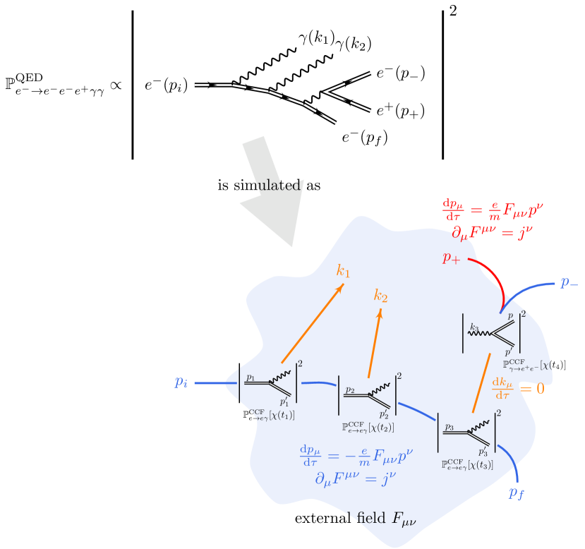
Figure 5: A general strong-field QED interaction, featuring the emission and creation of multiple photons and electron-positron pairs, is simulated ‘semiclassically’ by breaking it down into a chain of first-order processes (electrons, photons and positrons in blue, orange and red, respectively). Between these pointlike, instantaneous events, the particles follow classical trajectories guided by the Lorentz force: $\dot{p}_{\mu}=\pm eF_{\mu\nu}p^{\nu}/m$ and $\dot{X}^{\mu}=p^{\mu}/m$, dots denoting differentiation with respect to proper time $\tau$. Modification of the external field $F_{\mu\nu}$ is driven by the classical currents $j^{\mu}(x)=\pm(e/m)\int p^{\mu}(\tau)\delta^{4}[x-X(\tau)]\,\mathrm{d}\tau$. The probability rates and spectra for the first-order processes are those for a constant, crossed field, and depend on the local value of the quantum parameter $\chi(t)=\left|F_{\mu\nu}[X(t)]p^{\nu}(t)\right|/(mE_{\text{cr}})$.

The need to overcome these issues has motivated the development of numerical schemes that can model quantum processes at high multiplicity in general electromagnetic fields. In this article we characterize these schemes as ‘semiclassical’, by virtue of the fact that they factorize a QED process into a chain of first-order processes that occur in vanishingly small regions linked by classically determined trajectories, as illustrated in fig. 5. The rates and spectra for the individual interactions are calculated for the equivalent interaction in a constant, crossed field, which may be generalized to an arbitrary field configuration under certain conditions. The first key result is that, at $a_{0}\gg 1$, the formation length of a photon (or an electron-positron pair) is much smaller than the length scale over which the background field varies (see section I) and so emission may be treated as occurring instantaneously (Ritus, 1985). The second is that if $\chi^{2}\gg\left|\mathfrak{F}\right|,\left|\mathfrak{g}\right|$ and $\mathfrak{F}^{2},\mathfrak{g}^{2}\ll 1$, where $\mathfrak{F}=(\mathbf{E}^{2}-\mathbf{B}^{2})/E_{\text{cr}}^{2}$ and $\mathfrak{g}=\mathbf{E}\cdot\mathbf{B}/E_{\text{cr}}^{2}$ are the two field invariants, the probability of a QED process is well approximated by its value in a constant, crossed field: $P(\chi,\mathfrak{F},\mathfrak{g})\simeq P(\chi,0,0)+O(\mathfrak{F})+O(\mathfrak{g})$ [see Appendix B of Baier et al. (1998)]. The combination of the two is called the locally constant, crossed field approximation (LCFA). The first requires the laser intensity to be large, whereas the second requires the particle to be ultrarelativistic and the background to be weak (as compared to the critical field of QED). We will discuss the validity of these approximations, and efforts to benchmark them, in section III.3.

Within this framework, the laser-beam (or laser-plasma) interaction is essentially treated classically, and quantum interactions such as high-energy photon emission added by hand. The evolution of the electron distribution function $\mathcal{F}=\mathcal{F}(t,\mathbf{r},\mathbf{p})$, including the classical effect of the background field and stochastic photon emission, is given by (Elkina et al., 2011; Ridgers et al., 2017)

$$\frac{\partial\mathcal{F}}{\partial t}+\frac{\mathbf{p}}{\gamma m}\cdot\frac{\partial\mathcal{F}}{\partial\mathbf{r}}-e\left(\mathbf{E}+\frac{\mathbf{p}\times\mathbf{B}}{\gamma m}\right)\cdot\frac{\partial\mathcal{F}}{\partial\mathbf{p}}\\ =-\mathcal{F}\int W_{\gamma}(\mathbf{p},\mathbf{k}^{\prime})\,\mathrm{d}^{3}\mathbf{k}^{\prime}+\int\mathcal{F}(\mathbf{p}^{\prime})W_{\gamma}(\mathbf{p}^{\prime},\mathbf{p}^{\prime}-\mathbf{p})\,\mathrm{d}^{3}\mathbf{p}^{\prime},$$ (25)

where $W_{\gamma}(\mathbf{p},\mathbf{k}^{\prime})$ is the probability rate for an electron with momentum $\mathbf{p}$ to emit a photon with momentum $\mathbf{k}^{\prime}$. A direct approach to kinetic equations of this kind is to solve them numerically (Sokolov et al., 2010; Bulanov et al., 2013; Neitz and Di Piazza, 2013), or reduce them by means of a Fokker-Planck expansion in the limit $\chi\ll 1$ (Niel et al., 2018). However, the most popular is a Monte Carlo implementation of the emission operator [the right hand side of eq. 25], which naturally extends single-particle or particle-in-cell codes that solve for the classical evolution of the distribution function in the presence of externally prescribed, or self-consistent, electromagnetic fields (Duclous et al., 2011; Elkina et al., 2011). This method is discussed in detail in Ridgers et al. (2014); Gonoskov et al. (2015), so we only summarize it here for photon emission.

The electron distribution function is represented by an ensemble of macroparticles, which represent a large number $w$ of real particles ($w$ is often called the weight). The trajectory of a macroelectron between discrete emission events is determined solely by the Lorentz force. Each is assigned an optical depth against emission $T=-\log(1-R)$ for pseudorandom $0\leq R<1$, which evolves as $\frac{\mathrm{d}T}{\mathrm{d}t}=-W_{\gamma}$, where $W_{\gamma}$ is the probability rate of emission, until the point where it falls below zero. Emission is deemed to occur instantaneously at this point and $T$ is reset. The energy of the photon $\omega^{\prime}=\left|\mathbf{k}^{\prime}\right|$ is pseudorandomly sampled from the quantum emission spectrum $\frac{\mathrm{d}N_{\gamma}}{\mathrm{d}\omega}=\omega^{-1}\frac{\mathrm{d}\mathcal{P}_{\text{q}}}{\mathrm{d}\omega}(\chi,\gamma)$ [see eq. 19] and the electron recoil determined by the conservation of momentum $\mathbf{p}=\mathbf{p}^{\prime}+\mathbf{k}^{\prime}$ and the assumption that $\mathbf{k}^{\prime}\parallel\mathbf{p}$ if $\gamma\gg 1$. If desired, a macrophoton with the same weight as the emitting macroelectron can be added to the simulation. Electron-positron pair creation by photons in strong electromagnetic fields is modelled in an analogous way to photon emission (Ridgers et al., 2014; Gonoskov et al., 2015).

Thus there are two distinct descriptions of the electromagnetic field. One component is treated as a classical field (in a PIC code, this would be discretized on the simulation grid) and the other as a set of particles. In principle this leads to double-counting; however, as we discussed in section III.1, the former lies at much lower frequency than the photons that make up synchrotron emission, and has a distinct origin in the form of externally generated fields (such as a laser pulse) or the collective motion of a plasma. Coherent effects are much less important for the high-frequency components, which justifies describing them as particles (Gonoskov et al., 2015).

III.3 Benchmarking, extensions and open questions

The validity of the simulation approach discussed in section III.2 relies on the assumption that a high-order QED process in a strong electromagnetic background field may be factorized into a chain of first-order processes, each of which is well approximated by the equivalent process in a constant, crossed field. It is generally expected that this reduction works in scenarios where $a_{0}\gg 1$ and $\chi^{2}\gg\left|\mathfrak{F}\right|,\left|\mathfrak{g}\right|$ (Ritus, 1985; Baier et al., 1998). However, these asymptotic conditions do not give quantitative bounds on the error made by semiclassical simulations. As these are the primary tool by which we predict radiation reaction effects in high-intensity lasers, it is important that they are benchmarked and that the approximations are examined.

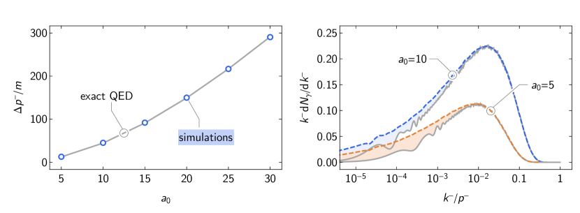
Figure 6: Comparison between exact QED (grey) and simulation results (blue and orange) for single nonlinear Compton scattering of an electron in a two-cycle, circularly polarized laser pulse: (left) the lightfront momentum loss as a function of laser amplitude $a_{0}$; and (right) exemplary photon spectra. Adapted from Blackburn et al. (2018).

One approach is to compare, directly, the predictions of strong-field QED and simulations. We focus here on results for single nonlinear Compton scattering (Harvey et al., 2015; Di Piazza et al., 2018; Blackburn et al., 2018), the emission of one and only one photon in the interaction of an electron with an intense, pulsed plane EM wave, by virtue of its close relation to radiation reaction. It is shown that the condition $a_{0}\gg 1$ is necessary, but not sufficient, for the applicability of the LCFA: we also require that $a_{0}^{3}/\chi\gg 1$ for interference effects to be suppressed (Dinu et al., 2016). These interference effects are manifest in the low-energy part of the photon emission spectrum $x=\omega^{\prime}/(\gamma m)<\chi/a_{0}^{3}$, as the formation length for such photons is comparable in size to the wavelength of the background field. Semiclassical simulations strongly overestimate the number of photons emitted in this part of the spectrum because they exclude nonlocal effects (Harvey et al., 2015; Di Piazza et al., 2018). Nevertheless, they are much more accurate with respect to the total energy loss (and therefore to radiation reaction), because this depends on the power spectrum, to which the low-energy photons do not contribute significantly (Blackburn et al., 2018). This is shown in fig. 6, which compares the predictions of exact QED and semiclassical simulations for an electron with $p^{-}_{0}/m\simeq 2\gamma_{0}=2000$ colliding with a two-cycle laser pulse with normalized amplitude $a_{0}$ and wavelength $\lambda=0.8~{}{\mu\mathrm{m}}$. There is remarkably good agreement between the two even for $a_{0}=5$.

An additional point of comparison in Blackburn et al. (2018) is the number of photons absorbed from the background field in the process of emitting a high-energy photon. This transfer of energy from the background field to the electron is required by momentum conservation. Without emission, there would be no such transfer of energy. This is consistent with the classical picture, in which plane waves do no work in the absence of radiation reaction. Strong-field QED calculations depend crucially on the fixed nature of the background field; however, for single nonlinear Compton scattering, near-total depletion of the field is predicted at $a_{0}\gtrsim 1000$ (Seipt et al., 2017). The theory must therefore allow for changes to the background (Ilderton and Seipt, 2018). Within the semiclassical approach, depletion is accounted for by the action of the classical currents through the $\mathbf{j}\cdot\mathbf{E}$ term in Poynting’s theorem. Quantum effects are manifest in how photon emission (and pair creation), modify those classical currents, as illustrated in fig. 5. In Blackburn et al. (2018), the classical work done on the electron is shown to agree well with the number of absorbed photons predicted by exact QED. This is consistent with the results of Meuren et al. (2016), which indicate that the ‘classical’ dominates the ‘quantum’ component of depletion, the latter associated with absorption over the formation length, if $a_{0}\gg 1$.

The failure of the semiclassical approach to reproduce the low-energy part of the photon spectrum arises from the localization of emission. Most notably, the number spectrum $\frac{\mathrm{d}N_{\gamma}}{\mathrm{d}\omega}=\omega^{-1}\frac{\mathrm{d}\mathcal{P}_{\text{q}}}{\mathrm{d}\omega}(\chi,\gamma)$ [see eq. 19] diverges as $\omega^{-2/3}$ as $\omega\to 0$. This can be partially ameliorated by the use of emission rates that take nonlocal effects into account. Di Piazza et al. (2019) suggest replacing the LCFA spectrum in the region $x\lesssim\chi/a_{0}^{3}$ with the equivalent, finite, result for a monochromatic plane wave, which they adapt for use in arbitrary electromagnetic field configurations. Ilderton et al. (2019) propose an approach based on formal corrections to the LCFA, in which the emission rates depend on the field gradients as well as magnitudes.

While the studies discussed above have given insight into the limitations of the LCFA, they do not examine the applicability of the factorization shown in fig. 5, as this requires by definition the calculation of a higher order QED process. At the time of writing, there are no direct comparisons of semiclassical simulations and strong-field QED for either double Compton scattering (emission of two photons) or trident pair creation (emission of a photon which decays into an electron-positron pair). Factorization, also called the cascade approximation, has been examined directly within strong-field QED for the trident process in a constant crossed field (King and Ruhl, 2013) and in a pulsed plane wave (Dinu and Torgrimsson, 2018; Mackenroth and Di Piazza, 2018). In the latter it is shown that at $a_{0}=50$ and an electron energy of 5 GeV, the error is approximately one part in a thousand.

The dominance of the cascade contribution makes it important to consider whether the propagation of the electron between individual tree-level process, as shown in fig. 5, is done accurately. In the standard implementation, this is done by solving a classical equation of motion including only the Lorentz force (Ridgers et al., 2014; Gonoskov et al., 2015). The evolution of the electron’s spin is usually neglected and emission calculated using unpolarized rates, such as eq. 19. King (2015) show that the accuracy of modelling double Compton scattering in a constant crossed field as two sequential emissions with unpolarized rates is better than a few per cent. There are, however, scenarios, where the spin degree of freedom influences the dynamics to a larger degree. Modelling these interactions with semiclassical simulations requires spin-resolved emission rates (Sokolov and Ternov, 1968; Seipt et al., 2018) and an equation of motion for the electron spin (Thomas, 1926; Bargmann et al., 1959). In a rotating electric field, as found at the magnetic node of an electromagnetic standing wave (Bell and Kirk, 2008), where the spin does not precess between emissions, the asymmetric probability of emission between different spin states leads to rapid, near-complete polarization of the electron population (Del Sorbo et al., 2017, 2018). Similarly, an electron beam interacting with a linearly polarized laser pulse can acquire a polarization of a few per cent (Seipt et al., 2018). To make this larger, it is necessary to break the symmetry in the field oscillations, which can be accomplished by introducing a small ellipticity to the pulse (Li et al., 2019), or by superposition of a second colour (Song et al., 2019; Chen et al., 2019; Seipt et al., 2019).

A more fundamental limitation on the applicability of the LCFA is that the emission rates are calculated at tree level only. The importance of loop corrections to the strong-field QED vertex grows as $\alpha\chi^{2/3}$ in a constant, crossed field (Morozov et al., 1981), leading to speculation that $\alpha\chi^{2/3}$ is the ‘true’ expansion parameter of strong-field QED (Narozhny, 1980). When $\chi\simeq 1600$, this parameter becomes of order unity and the meaning of a perturbative expansion in the dynamical electromagnetic field breaks down. The recent review by Fedotov (2017) has prompted renewed interest in this regime; recent calculations of the one-loop polarization and mass operators (Podszus and Di Piazza, 2019) and photon emission and helicity flip (Ilderton, 2019) in a general plane-wave background have confirmed that the power-law scaling of radiative corrections pertains strictly to the high-intensity limit $a_{0}^{3}/\chi\gg 1$. In the high-energy limit, radiative corrections grow logarithmically, as in ordinary (i.e., non-strong-field) QED (Podszus and Di Piazza, 2019; Ilderton, 2019).

The difficulty in probing the regime $\alpha\chi^{2/3}\gtrsim 1$ is the associated strength of radiative energy losses, which suppress $\gamma$ and so $\chi$ (Fedotov, 2017). Overcoming this barrier at the desired $\chi$ requires the interaction duration to be very short. The beam-beam geometry proposed by Yakimenko et al. (2019) exploits the Lorentz contraction of the Coulomb field of a compressed (100 nm), ultrarelativistic (100 GeV) electron beam, which is probed by another beam of the same energy. In the laser-electron-beam scenario considered by Blackburn et al. (2019), collisions at oblique incidence are proposed for reaching $\chi\gtrsim 100$, exploiting the fact that the diameter of a laser focal spot is typically much smaller than the duration of its temporal profile. Even higher $\chi$ is reached in the combined laser-plasma, laser-beam interaction proposed by Baumann and Pukhov (2019). While it seems possible to approach the fully nonperturbative regime experimentally, albeit for extreme collision parameters, there is no suitable theory at $\alpha\chi^{2/3}\gtrsim 1$, and quantitative predictions are lacking in this area.

IV Experimental geometries, results and prospects

IV.1 Geometries

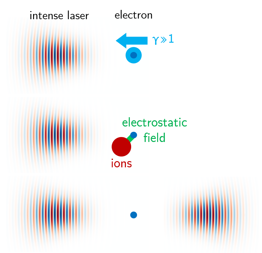
Figure 7: Tightly focussed laser pulses can ponderomotively expel electrons from the region of highest intensity, suppressing the onset of radiation-reaction and quantum effects. There are three typical experimental geometries that ensure that energetic electrons are embedded in strong EM fields as desired: (top) laser–particle-beam, (centre) laser-plasma, and (bottom) laser-laser.

It may be appreciated that the radiation-reaction and quantum effects under consideration here, as particle-driven processes, can only become important if electrons or positrons are actually embedded within electromagnetic fields of suitable strength. However, the estimates in section I were made for a plane EM wave, in which case the electron is guaranteed to interact with the entire wave, including the point of highest intensity. In reality, such intensities are reached by compressing the laser energy into ultrashort pulses (Strickland and Mourou, 1985) that are focussed to spot sizes close to the diffraction limit (Bahk et al., 2004; Sung et al., 2017; Kiriyama et al., 2018). The steep spatiotemporal gradients in intensity that result mean that laser pulses can ponderomotively expel electrons from the focal region, in both vacuum (Malka et al., 1997; Thévenet et al., 2016) and plasma (Esarey et al., 2009), curtailing the interaction long before the particles experience high $a_{0}$ or $\chi$.

The literature contains many possible experimental configurations designed to explore or exploit radiation reaction and quantum effects. These configurations can be divided, broadly, into three categories, based on how they ensure the spatial coincidence between particles and strong fields. Figure 7 illustrates the three categories. In the first (laser–particle-beam), the electrons are accelerated to ultrarelativistic energies before they encounter the laser pulse. The effective ‘mass increase’ makes the beam rigid and so it passes through the entirety of the laser pulse, avoiding substantial deflection and ensuring that it is exposed to the strongest electromagnetic fields. Concretely, the ponderomotive force is suppressed at high $\gamma$: $\mathrm{d}\langle\mathbf{p}\rangle/\mathrm{d}t=-m\mathbf{\nabla}\langle a^{2}\rangle/(2\langle\gamma\rangle)$, where $\langle\cdot\rangle$ denotes a cycle-averaged quantity (Quesnel and Mora, 1998). It should be noted that it is possible for radiation reaction to amplify this force to the point that it can prevent an arbitrarily energetic electron from penetrating the laser field (Zhidkov et al., 2014; Fedotov et al., 2014); however, this requires $a_{0}\gtrsim 300$, far in excess of what it is available at present. In today’s high-intensity lasers, ultrarelativistic electrons can reach the nonlinear quantum regime $\chi\sim 1$ even for $a_{0}\sim 10$ (see fig. 2).

In the second (laser-plasma), the electrons are electrostatically bound to a population of ions, which are substantially more massive and therefore less mobile. Large-scale displacement of the electrons away from the laser fields is then suppressed by the emergence of plasma fields. If the plasma is overdense, i.e. opaque to the laser light, then only electrons in a thin layer near the surface experience the full laser intensity and are accelerated to relativistic energies. However, the high density of electrons in this region means that a significant fraction of the laser energy is converted to high-energy radiation, leading to, for example, dense bursts of $\gamma$ rays and positrons (Ridgers et al., 2012; Brady et al., 2012), reduced efficiency of ion acceleration (Tamburini et al., 2010) and the generation of long-lived quasistatic magnetic fields (Liseykina et al., 2016). If the target is close to underdense, by contrast, the laser can propagate through the plasma bulk and the interaction is volumetric in nature. The combination of laser and induced plasma fields, as well as radiation reaction, leads to confinement and acceleration of the electrons, and copious emission of radiation (Stark et al., 2016; Zhu et al., 2016; Vranic et al., 2018).

Finally, electrons can be trapped in the collision of more than one laser pulse (laser-laser), where they interact with an electromagnetic standing, rather than travelling, wave (Bulanov et al., 2010). Radiation reaction induces a rich set of dynamics in this configuration (Ji et al., 2014; Gonoskov et al., 2014; Esirkepov et al., 2015; Kirk, 2016). The fact that standing waves can do work in reaccelerating the particles after they recoil means that, at intensities $\gtrsim 10^{24}~{}\mathrm{W}\text{cm}^{-2}$, the emitted photons seed avalanches of electron-positron pair creation (Bell and Kirk, 2008); this intensity threshold is lowered in suitable multibeam setups (Gelfer et al., 2015; Vranic et al., 2017; Gong et al., 2017). The case of optimal focussing is achieved in a dipole field (Bassett, 1986), where the peak $a_{0}\simeq 780\mathcal{P}^{1/2}[\text{PW}]$ (Gonoskov et al., 2012). Such extreme intensities, at moderate power, are the reason this configuration has been studied as means of high-energy photon production (Gonoskov et al., 2017; Magnusson et al., 2019).

It is important to note that the distinction between the three categories defined here is not absolute. Mixing between them occurs in, for example, the interaction of a linearly polarized laser pulse with relativistically underdense plasma: here re-injected electron synchrotron emission, the radiation emission when electrons are pulled backwards into the oncoming laser by a charge-separation field (Brady et al., 2012), exhibits features of both the ‘laser-plasma’ and ‘laser-beam’ geometries. Furthermore, the exponential growth of particle number in a QED cascade driven by multiple laser pulses can create an electron-positron plasma of sufficient density to shield the interior from the laser pulse (Grismayer et al., 2016), leading to a transition between the ‘laser-laser’ and ‘laser-plasma’ categories. Twin-sided illumination of a foil has features of both ab initio (Zhang et al., 2015).

IV.2 ‘All-optical’ colliding beams

This paper focuses on the first of the three configurations discussed in section IV.1, laser–particle-beam, for the reason that it allows $\chi>0.1$ to be reached at lower $a_{0}$ than would be required in a laser-plasma or laser-laser interaction. As is shown in fig. 2 and by eq. 6, given a 500-MeV electron beam, quantum effects on radiation reaction can be reached even at an intensity of $10^{21}~{}\mathrm{W}\text{cm}^{-2}$. The colliding beams geometry therefore represents a promising first step towards experimental exploration of the radiation-dominated or nonlinear quantum regimes.

Thus far we have not specified the source of ultrarelativistic electrons. The theoretical description of the interaction does not depend on the source, of course, but it is of immense practical importance. Furthermore, the characteristics of the source (its energy, bandwidth, emittance, etc.) are key determining factors in the viability of measuring radiation-reaction or quantum effects. For example, the fact that electron beam energy spectra are expected to broaden due to stochastic effects makes the variance of the spectrum, $\sigma^{2}$, an attractive signature of the quantum nature of radiation reaction (Neitz and Di Piazza, 2013; Vranic et al., 2016a). However, such broadening can occur classically in the interaction of an electron beam with a focussed laser pulse, because components of the beam can encounter different intensities and therefore lose different amounts of energy (Harvey et al., 2016). Thus a crucial role is played by the initial energy spread and size of the incident electron beam (Samarin et al., 2017).

In fact, it was pioneering experiments with a conventional, radio-frequency (RF), linear accelerator that provided the first demonstration of nonlinear quantum effects in a strong laser field: nonlinearities were measured in Compton scattering (Bula et al., 1996) and Breit-Wheeler electron-positron pair creation (Burke et al., 1997) in Experiment 144 at the Stanford Linear Accelerator (SLAC) facility. In this experiment, the $46.6$ GeV electron beam was collided with a laser pulse of intensity $1.3\times 10^{18}~{}\mathrm{W}\text{cm}^{-2}$, duration $1.4$ ps and wavelength $527$ nm ($a_{0}\simeq 0.4$, $\chi=0.3$) (Bamber et al., 1999). The pair creation mechanism was reported to be the multiphoton Breit-Wheeler process, as $n=4$ laser photons were required in addition to each multi-GeV $\gamma$ ray (emitted by the electron in Compton scattering) to overcome the mass threshold. In total, $106\pm 14$ positrons were observed over the series of 22,000 laser shots. The yield was strongly limited because, even though the electron energy was sufficient to reach a quantum parameter $\chi\sim 0.3$, in the regime $a_{0}\ll 1$, the pair creation probability is suppressed as $a_{0}^{2n}$, where $n$, the number of participating photons, was found to be $n\simeq 5$ (Burke et al., 1997). Similarly, the photon emission process was weakly nonlinear, with harmonics of the fundamental Compton energy up to $n=4$ observed (Bula et al., 1996). At the time of writing, this experiment had yet to be repeated at a conventional linear accelerator, though concrete proposals have now been made to do so at DESY (Abramowicz et al., 2019) and FACET-II (Meuren, 2019). While the electron beams will be less energetic ($17.5$ and $10$ GeV respectively), the laser intensity will be higher ($2\lesssim a_{0}\lesssim 10$), so the transition from the multiphoton to the tunnelling regimes could be explored.

One of the challenges that must be overcome in realizing these experiments is that, as discussed in section IV.1, lasers reach high intensity by focussing and compressing energy into a small spatiotemporal volume. Thus the region in which the electromagnetic fields are strong is only a few microns in radius, assuming diffraction-limited focussing and optical drivers ($\omega\sim 1$ eV), which is much smaller than the size of the focussed electron beam from a conventional accelerator. This limits the number of electrons that interact with the laser, reducing the relevant signal, as well as making the alignment and timing of the beams more difficult (Samarin et al., 2017). In the ‘all-optical’ geometry, these are overcome by using a dual-laser setup (Bulanov et al., 2011a): one laser provides the high-intensity ‘target’, and the other is used to accelerate electrons in a plasma wakefield.

Laser-driven wakefield acceleration has undergone remarkable progress over the last two decades: from the first quasi-monoenergetic relativistic beams (Mangles et al., 2004; Geddes et al., 2004; Faure et al., 2004), they now produce electron beams with near- to multi-GeV energies (Kneip et al., 2009; Wang et al., 2013; Gonsalves et al., 2019). Briefly, an intense laser pulse travels through a low-density plasma, exciting, via its ponderomotive effect, a trailing nonlinear plasma wave that traps and accelerates electrons (Esarey et al., 2009). As the medium is a plasma, already ionized and therefore immune to electrostatic breakdown, the accelerating gradients are much higher than in a conventional RF accelerator: GeV energies can be reached in only a few centimetres of propagation. Furthermore, as the size of the accelerating structure is only a few microns (at typical plasma densities $n_{e}\sim 10^{18}~{}\text{cm}^{-3}$, the plasma wavelength $\sim 20~{}{\mu\mathrm{m}}$), the electron beams produced in wakefield acceleration are similarly micron-scale, with durations of order 10 fs.

Besides the high energy and the small size of the electron beam, we have the intrinsic synchronizations of the electron beam with the accelerating laser pulse, and of the accelerating laser pulse with the target laser pulse, if the two emerge from amplifier chains that are seeded by the same oscillator. Thus the ‘all-optical’ laser-electron-beam collision is promising as a compact source of bright, ultrashort bursts of high-energy $\gamma$ rays (Chen et al., 2013; Sarri et al., 2014; Yan et al., 2017). Now, with advances in laser technology, a multibeam facility is capable of reaching the radiation-reaction and nonlinear quantum regimes. Recently two such experiments were performed using the Gemini laser at the Rutherford Appleton Laboratory (Cole et al., 2018; Poder et al., 2018), a dual-beam system that delivers twin synchronized pulses of duration $45$ fs and energy $\sim 10$ J, with a peak $a_{0}\simeq 20$: we discuss these experiments in detail in section IV.3. Upcoming laser facilities, such as Apollon (Papadopoulos et al., 2016) or ELI (Weber et al., 2017; Gales et al., 2018), aim for laser-electron collisions at even higher intensity: see, for example, Lobet et al. (2017) for simulations of dual-beam interactions at $a_{0}\simeq 200$.

Not all high-intensity laser facilities have dual-beam capability. An alternative all-optical configuration, introduced by Ta Phuoc et al. (2012), employs a single laser pulse as accelerator and target: a foil is placed at the end of a gas jet, into which a laser is focussed to drive a wakefield and accelerate electrons; when the laser pulse reaches the foil, it is reflected from the ionized surface back onto the trailing electrons. This guarantees temporal and spatial overlap of the two beams, but precludes the possibility of separately optimizing the two laser pulses; in Ta Phuoc et al. (2012) the electron energies $\simeq 100$ MeV and the peak $a_{0}\simeq 1.5$, so radiation reaction effects were negligible. Simulations of similar single-pulse geometries predict the efficient production of multi-MeV photons at $a_{0}>50$ (Huang et al., 2019) and electron-positron pairs at $a_{0}\gtrsim 300$ (Liu et al., 2016; Gu et al., 2018).

IV.3 Recent results

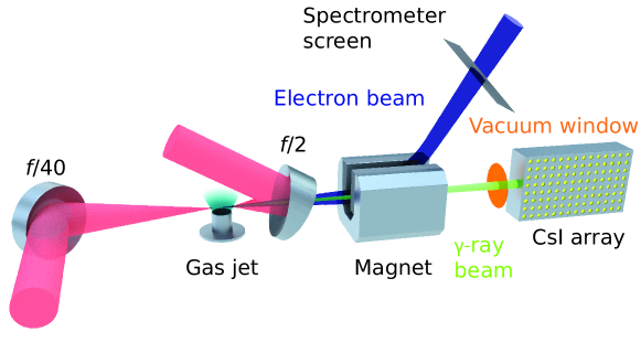
Figure 8: Layout of an all-optical colliding-beams experiment. A hole in the short-focal-length ($F/2$) optic allows for counterpropagation of the electron beam, which is accelerated by a laser wakefield in a gas jet, and the high-intensity laser pulse. The decelerated electrons, the $\gamma$ rays they emit in the collision, and the accelerating laser pulse, pass through this hole before being blocked or diagnosed as appropriate. The collision is timed to occur close to the rear of the gas jet (on the right-hand side, as viewed in the figure), before the electron beam can diverge significantly, which maximizes overlap between the beams. Reproduced from Cole et al. (2018).

The Gemini laser of the Central Laser Facility (Rutherford Appleton Laboratory, UK) is a petawatt-class dual-beam system (Hooker et al., 2006), well-suited for the all-optical colliding beams experiments discussed in section IV.2. It delivers two, synchronized, linearly polarized laser pulses of duration $45~{}\mathrm{fs}$, energy 10 J and wavelength $0.8~{}{\mu\mathrm{m}}$. Available focussing optics include long-focal-length mirrors ($F/20$ and $F/40$) for laser-wakefield acceleration and, most importantly, a short-focal-length ($F/2$) off-axis parabolic mirror with an $F/7$ hole in its centre (Cole et al., 2018; Poder et al., 2018). The latter allows for direct counterpropagation of the two laser beams, the geometry in which $\chi$ is largest (see eq. 17): the more weakly focussed laser that drives the wakefield passes through the hole and is subsequently blocked, avoiding backreflection in the amplifier chains; the accelerated electron beam, and any radiation produced in the collision with the tightly focussed laser, can pass through to reach the diagnostics. Both the experiments that will be described in this section used this geometry, which is illustrated in fig. 8, but with different electron acceleration stages.

In Cole et al. (2018), the accelerating laser pulse was focussed onto the leading edge of a supersonic helium gas jet, producing a ${\sim}15$ mm plasma acceleration stage with peak density $n_{e}\simeq 3.7\times 10^{18}~{}\text{cm}^{-3}$. The use of a gas jet allowed the second laser pulse to be focussed close to the point where the electron beam emerges from the plasma (at the rear edge), so the collision between electron beam and laser pulse took place when the former was much smaller than the latter (approximately $1~{}{\mu\mathrm{m}}^{2}$ rather than $20~{}{\mu\mathrm{m}}^{2}$, which includes the effect of a systematic time delay between the two). The advantages of using a gas cell, as in Poder et al. (2018), are the higher electron beam energies and significantly better shot-to-shot stability. However, in this case, the second laser pulse must be focussed further downstream of the acceleration stage (approximately 1 cm), by which point the electron beam has expanded to become comparable in size to the laser. Thus full 3D simulations were required for theoretical modelling of the interaction, whereas 1D (plane-wave) simulations were sufficient in Cole et al. (2018).

Fluctuations in the pointing and timing of the two lasers, as well as systematic drifts in the latter, mean that the overlap between electron beam and target laser pulse varies from shot to shot. It is helpful, therefore, to gather as large a dataset as possible (with the second, high-intensity, laser pulse both on and off), in which case high-repetition-rate laser systems are at a clear advantage. However, this is not nearly so important as being able to identify ‘successful’ collisions when they occur; even a small set of collisions ($N\sim 10$) can provide statistically significant evidence of radiation reaction when this is done. This speaks to the importance of measuring both the electron and $\gamma$-ray spectra on a shot-to-shot basis; identifying coincidences between the two provides stronger evidence of radiation reaction than could be obtained by either alone.

In Cole et al. (2018), successful shots were distinguished by measuring the total signal in the $\gamma$-ray detector $S_{\gamma}\propto N_{e}a^{2}\langle\gamma^{2}\rangle$ (background-corrected), where $N_{e}$ is the total number of electrons in the beam, $\langle\gamma^{2}\rangle$ their mean squared Lorentz factor, and $a$ an overlap-dependent, effective value for $a_{0}$ (the former two can be extracted from the measured electron spectra). Over a sequence of 18 shots (eight beam-on, i.e. with the $f/2$ beam on, ten beam-off), four were measured with a normalized CsI signal, $\hat{S}_{\gamma}=S_{\gamma}/(N_{e}\langle\gamma^{2}\rangle)\propto a^{2}$, four standard deviations above the background level. These four also had electron beam energies below 500 MeV (as identified by a strong peak feature in the measured spectra), whereas the ten beam-off shots had a mean energy of $550\pm 20$ MeV. The probability of measuring four or more beams with energy below 500 MeV in a sample of eight, given this fluctuation alone, is approximately 10%. However, the probability that four beams have this lower energy and a significantly higher $\gamma$-ray signal is the considerably smaller 0.3%.

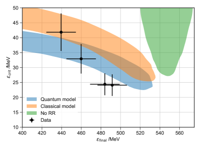
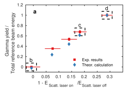
Figure 9: Experimental evidence of radiation reaction: (left) in Cole et al. (2018), the post-collision electron beam energies and critical energies of the $\gamma$-ray spectra (black points), are consistent with theoretical simulations that include radiation reaction, with slightly better agreement for the stochastic model; (right) in Poder et al. (2018), the fractional reduction in the total electron beam energy is correlated with the total $\gamma$-ray signal, with the best agreement with theory given by the ‘modified classical’ model (see section III.1). Details are given in the main text.

Statistically significant evidence of radiation reaction was obtained by correlating the electron beam energy with the critical energy of the $\gamma$-ray spectrum $\varepsilon_{\text{crit}}$, a parameter characterizing the hardness of the spectrum. This was accomplished by fitting the depth-resolved scintillator output to a parametrized spectrum $dN_{\gamma}/d\omega\propto\omega^{-2/3}\exp(-\omega/\varepsilon_{\text{crit}})$, having first characterized its response to monoenergetic photons in the energy range $2<\omega[\text{MeV}]<500$ with Geant4 simulations (see details in Behm et al. (2018)). This choice of parametrization approximately reproduces a synchrotron-like spectral shape, with an exponential rollover at high energy and a scaling like $\omega^{-2/3}$ at low energy. The four successful shots demonstrate a negative correlation between the final electron energy and $\varepsilon_{\text{crit}}$, as is shown in fig. 9; this is consistent with radiation-reaction effects, as the hardest photon spectra should come from electron beams that have lost the most energy. The probability to observe this negative correlation and to have electron energy lower than 500 MeV on all four successful shots is 0.03%, which qualifies, under the usual three-sigma threshold, as evidence of radiation reaction.

Simulations of the collision confirmed that the critical energies and electron energy loss were consistent with theoretical expectations of radiation reaction. The coloured regions in fig. 9 give the areas in which 68% (i.e. one sigma) of results would be found for a large ensemble of ‘numerical experiments’, given the measured fluctuations in the pre-collision electron energy spectra and the collision $a_{0}$, and under specific models of radiation reaction. The results exclude the ‘no RR’ model, in which the electrons radiate, but do not recoil. They are more consistent with the stochastic, quantum model discussed in section III.2 than the deterministic, classical model of Landau-Lifshitz: however, it is important to note that both models are consistent with the data at the two-sigma level. Subsequent analysis has confirmed that the ‘modified classical’ model discussed in section III.1, which includes the quantum suppression factor $g(\chi)$, given in eq. 20, but not the stochasticity of emission, gives practically the same region as the quantum model (Cole, 2018), as is stated in Cole et al. (2018). This is because the electron beam energy effectively parametrizes the mean of the spectrum, the evolution of which depends only on $g(\chi)$ according to eq. 23; to see stochastic effects, we must consider instead the width of the distribution (Neitz and Di Piazza, 2013; Vranic et al., 2016a; Ridgers et al., 2017). Given electron beams with narrower initial energy spectra, it would be possible to identify stochastic effects (or their absence) by correlating the mean and variance of the final electron energy spectra (Arran et al., 2019).

Evidence of radiation reaction was also obtained in the experiment reported by Poder et al. (2018), by a complementary form of analysis. The total CsI signal was used to discriminate successful collisions: the signal normalized to the total energy in a reference (beam-off) shot $S_{\gamma}/(N_{e}\langle\gamma\rangle)$ was observed to be linearly correlated with the percentage energy loss of the electron beam (as compared against a reference beam, see fig. 9). Three shots were selected as exemplary cases of poor, moderate and strong overlap, according to these two values, with corresponding strength of radiation-reaction effects. This shots are labelled (b), (c) and (d) respectively in the right-hand panel of fig. 9. The analysis then focussed on comparison of the measured electron energy spectra against those predicted by simulations under various models of radiation reaction. These comparisons showed that the Landau-Lifshitz equation, i.e. classical radiation reaction, overestimated the energy loss, with a quality of fit of $R^{2}=0.87$. Simulations with the ‘modified classical’ model improved the agreement to $R^{2}=0.96$; this was found to give better agreement than the fully stochastic model, in which case $R^{2}=0.92$. This discrepancy was attributed to possible failure of the LCFA as the collision $a_{0}\simeq 10$. Nevertheless, by considering the detailed shape of electron energy spectra, it was possible to find clear evidence of radiation reaction, as well as signatures of quantum corrections.

V Summary and outlook

Let us now consider the relation between the results of these two experiments discussed in section IV.3. Both present clear evidence that radiation reaction, in some form, has taken place. The reduction in the electron energies, the total $\gamma$-ray signal, and, in Cole et al. (2018), the spectral shape of the latter, are all broadly consistent with each other. The differences arise in the comparison of different models of radiation reaction, bearing in mind that, in the regime where $\chi\simeq 0.1$, $a_{0}\simeq 10$, quantum corrections are expected to be non-negligible, but not large, and the intensity is not so large that the LCFA is beyond question. The use of simulations that rely on this approximation is, however, necessary because the number of photons emitted, per electron in the beam, is much larger than unity, and therefore an exact calculation from QED is intractable at present (see section III.3). In Cole et al. (2018), the shot-to-shot fluctuations in the electron beam energy and alignment, and the fact that the electron spectrum is analyzed by means of a single value rather than its complete shape, mean that all three models (classical, modified classical, and quantum) are not distinguishable from each other at level of two standard deviations. At the one-standard-deviation level, the two models that include quantum corrections provide better agreement.

Poder et al. (2018), with significantly more stable electron beams, are able to confirm that the classical model is not consistent with the data either. However, the fact that neither the modified classical or quantum models provide a very good fit to the data leaves open the question of whether it is the failure of the LCFA or, as they state, “incomplete knowledge of the local properties of the laser field.” Accurate determination of the initial conditions, in both the electron beam and the laser pulse, will be of unquestioned importance for upcoming experiments that aim to discern the properties of radiation reaction in strong fields. It will be vital to characterize the uncertainties in both the experimental conditions and the theoretical models in our simulations, which are inevitably based on certain approximations.

Nevertheless, these results demonstrate the capability of currently available high-intensity lasers to probe new physical regimes, where radiation reaction and quantum processes become the important, if not dominant, dynamical effects. These experiments provide vital data in the unexplored region of parameter space $\chi\gtrsim 0.1$, $a_{0}\gg 1$ (see fig. 2), allowing us to examine critically our theoretical and simulation approaches to the modelling of particle dynamics in strong electromagnetic fields. The current mismatch between simulations and experimental data has prompted, and will continue to prompt, new ideas in how to resolve the discrepancy: from the development of analysis techniques that are robust against shot-to-shot fluctuations (Baird et al., 2019; Arran et al., 2019), to improved simulation methodologies (Di Piazza et al., 2019; Ilderton et al., 2019). These are accompanied by renewed examination of the approximations underlying our simulations (see section III.3). The development of theoretical approaches that can go beyond the plane-wave configuration, the background field approximation, or low multiplicity, in strong-field QED is vital if this theory is to be applied directly in experimentally relevant scenarios. There is also undoubtedly a need to gather more experimental data and explore a wider parameter space, increasing the electron beam energy and laser intensity, i.e. $\chi$ and $a_{0}$. Not only will this make radiation reaction and quantum corrections more distinct, it will also allow us to measure nonlinear electron-positron pair creation by the $\gamma$ rays emitted by the colliding electron beam (Sokolov et al., 2010; Bulanov et al., 2013; Lobet et al., 2017; Blackburn et al., 2017), a strong-field QED process without classical analogue. Such findings will underpin the study of particle and plasma dynamics in strong electromagnetic fields for many years to come.