Origin of the Magnetic Spin Hall Effect: Spin Current Vorticity in the Fermi Sea

Abstract

The interplay of spin-orbit coupling (SOC) and magnetism gives rise to a plethora of charge-to-spin conversion phenomena that harbor great potential for spintronics applications. In addition to the spin Hall effect, magnets may exhibit a magnetic spin Hall effect (MSHE), as was recently discovered [Kimata et al., Nature 565, 627-630 (2019)]. To date, the MSHE is still awaiting its intuitive explanation. Here we relate the MSHE to the vorticity of spin currents in the Fermi sea, which explains pictorially the origin of the MSHE. For all magnetic Laue groups that allow for nonzero spin current vorticities the related tensor elements of the MSH conductivity are given. Minimal requirements for the occurrence of a MSHE are compatibility with either a magnetization or a magnetic toroidal quadrupole. This finding implies in particular that the MSHE is expected in all ferromagnets with sufficiently large SOC. To substantiate our symmetry analysis, we present various models, in particular a two-dimensional magnetized Rashba electron gas, that corroborate an interpretation by means of spin current vortices. Considering thermally induced spin transport and the magnetic spin Nernst effect in magnetic insulators, which are brought about by magnons, our findings for electron transport can be carried over to the realm of spincaloritronics, heat-to-spin conversion, and energy harvesting.

I From the conventional to the magnetic spin Hall effect

The spin Hall effect (SHE) Sinova et al. (2015) and its inverse are without doubt important discoveries Kato et al. (2004); Wunderlich et al. (2005); Saitoh et al. (2006); Valenzuela and Tinkham (2006); Zhao et al. (2006) in the field of spintronics Wolf et al. (2001); Žutić et al. (2004). They serve not only as ‘working horses’ for generating and detecting spin currents Jungwirth et al. (2012) but also as key ingredients in spin-orbit torque devices for electric magnetization switching Chernyshov et al. (2009); Liu et al. (2011, 2012). Compared to spin-transfer torque devices Slonczewski (1996); Berger (1996); Ralph and Stiles (2008); Brataas et al. (2012); Khvalkovskiy et al. (2013), spin-orbit torque devices are faster, more robust, and consume less power upon operation Gambardella and Miron (2011); Jabeur et al. (2014); Prenat et al. (2016); for a recent review see Ref. Li et al., 2018.

While the anomalous Hall effect (AHE) in a magnet Nagaosa et al. (2010) produces a transverse charge current density upon applying an electric field $\boldsymbol{E}$, the SHE in a nonmagnet produces a transverse spin current density $\langle\boldsymbol{j}^{\gamma}\rangle=\underline{\sigma}^{\gamma}\boldsymbol{E}$ ($\gamma=x,y,z$ indicates the transported spin component). Mathematically, the SHE is quantified by the antisymmetric part of the spin conductivity tensor $\underline{\sigma}^{\gamma}$. For example, the $\sigma^{z}_{xy}$ element comprises $z$-polarized spin currents in $x$ direction as a response to an electric field in $y$ direction.

In a simple picture, the intrinsic SHE S. Murakami and Zhang (2003); Sinova et al. (2004) is explained by spinning electrons that experience a spin-dependent Magnus force caused by spin-orbit coupling (SOC). It appears as if ‘built-in’ spin-dependent magnetic fields evoke spin-dependent Lorentz forces that result in a transverse pure spin current. The extrinsic SHE Dyakonov and Perel (1971); Hirsch (1999); Zhang (2000) is covered by Mott scattering at defects Mott (1929).

Since the SHE does not rely on broken time-reversal symmetry (TRS), it is featured in nonmagnetic metals Guo et al. (2008) or semiconductors Kato et al. (2004). Imposing few demands on a material’s properties, a SHE can be expected in any material with sufficiently large SOC (or, instead of SOC, with a noncollinear magnetic texture Zhang et al. (2018a)). From a mathematical perspective the existence of an SHE can be traced to the transformation behavior of the sum

$$\sigma_{xy}^{z}-\sigma_{yx}^{z}+\sigma_{yz}^{x}-\sigma_{zy}^{x}+\sigma_{zx}^{y}-\sigma_{xz}^{y},$$ (1)

of antisymmetric spin conductivity tensor elements traditionally associated with a SHE (applied field, current flow direction, and transported spin component are mutually orthogonal). Taking time-reversal evenness for granted, this sum behaves like an electric monopole (space-inversion even, scalar). For there are no crystalline symmetries (reflections, rotations, inversions) that could render such an object zero, a SHE can basically occur in any material. For the rest of this Paper, we refer to this SHE as ‘conventional SHE.’

To combine the virtues of transverse spin transport with magnetic recording, the conventional SHE was studied in magnetic materials with broken TRS (ferromagnets Miao et al. (2013); Taniguchi et al. (2015); Tian et al. (2016); Wu et al. (2017); Das et al. (2017); Humphries et al. (2017); Amin et al. (2018); Gibbons et al. (2018); Bose et al. (2018); Baek et al. (2018); Omori et al. (2019); Amin et al. (2019); Qu et al. (2019); Wang et al. (2019) or antiferromagnets Železný et al. (2017, 2018); Zhang et al. (2018a); Chen et al. (2018); Kimata et al. (2019)), which revealed various phenomena associated with the interplay of SOC and magnetism. For example, ferromagnetic metals exhibit an (inverse) conventional SHE Miao et al. (2013); unaffected by magnetization reversal Tian et al. (2016) it is time-reversal even.

Since charge currents in ferromagnets are intrinsically spin-polarized, transverse AHE currents are spin-polarized as well and are used to generate spin torques Taniguchi et al. (2015); Das et al. (2017). This effect is sometimes referred to as anomalous SHE Das et al. (2017), but is fundamentally a conventional SHE. Since these spin currents are tied to the AHE charge currents, the spin accumulations brought about by this effect can be manipulated by varying the magnetization direction Gibbons et al. (2018); Amin et al. (2019); Qu et al. (2019). This finding can be understood by considering symmetries. For a nonmagnetic cubic material only the components in Eq. (1) are allowed nonzero. In contrast, a ferromagnetic material magnetized along a generic direction has a lower symmetry: there are no constraints that prohibit ‘populating’ the entire spin conductivity tensor. Upon manipulation of the magnetization, an electric field in, say, $y$ direction causes an arbitrary spin polarization flowing in, e. g., $x$ direction. This offers greater versatility for spin torque applications than the conventional SHE in nonmagnetic cubic materials (nonmagnetic and noncubic materials also admit of greater versatility and nontraditional tensor elements Wimmer et al. (2015); Seemann et al. (2015); MacNeill et al. (2016); Zhou et al. (2019), but they do not offer external means, such as magnetization, to manipulate spin polarizations).

Since TRS is intrinsically broken in magnets, one expects that spin accumulations brought about by transverse spin currents have two components, one that does not reverse under magnetization reversal (we will refer this effect as SHE, a subset of which is the conventional SHE) and a second that is reversed under magnetization reversal. This opposite behavior under time reversal causes different restrictions imposed by the magnetic point-group symmetry Seemann et al. (2015); Železný et al. (2017) on the two types of spin accumulations. In particular, the latter magnetism-induced accumulations do not have to be parallelly polarized to the SHE spin accumulations. Such signatures were observed in Ref. Humphries et al., 2017.

The disentanglement of spin current contributions odd or even under time reversal has been elucidated in Ref. Železný et al., 2017. In essence, the spin conductivity tensor in Kubo transport theory is decomposed into a time-reversal even part and a time-reversal odd part. Upon disregarding spin-dependent scattering, skew scattering, and side jumps, the time-reversal even part is associated with ‘intrinsic’ contributions to the spin conductivity, a contribution given solely in terms of band structure properties (in the so-called clean limit) Železný et al. (2017). Likewise, the time-reversal odd part is associated with ‘extrinsic’ contributions that depend on relaxation times Železný et al. (2017). The latter gives rise to the magnetism-induced effects. In systems with low symmetry both parts contribute to all components of $\underline{\sigma}^{\gamma}$ and, in particular, to its antisymmetric part: the time-reversal even part gives rise to the SHE and the odd part to the magnetic spin Hall effect (MSHE) Železný et al. (2017); Chen et al. (2018); Kimata et al. (2019).

The MSHE has recently been experimentally detected in the noncollinear antiferromagnet Mn₃Sn Kimata et al. (2019), and the aforementioned results of Ref. Humphries et al., 2017 on ferromagnets can also be considered proof of the MSHE (in Ref. Davidson et al., 2019 referred to as ‘transverse SHE with spin rotation’). Although instances of the MSHE have been identified, an intuitive picture that explains how and under which circumstances this effect comes about is missing.

II Chiral vortices of spin currents: Summary of this Paper

We offer a vivid microscopic picture of the MSHE by relating it to the spin current vorticity (SCV) of the Fermi sea or, equivalently, to the circulation of spin currents about the Fermi surface.

In a rough draft, magnetic materials feature spin current whirlpools (or vortices) in reciprocal space for each of the three spin directions $\gamma=x,y,z$; as usual for angular quantities, we denote the axis of a vortex by a vector $\boldsymbol{\omega}^{\gamma}$. Similar to water whirlpools (in real space), whose handedness leads to an asymmetric deflection of plane water waves, the spin current whirlpools (in reciprocal space) cause an asymmetric deflection of the respective spin component. Since the spin current vortices occur in reciprocal space, they are delocalized in real space and, hence, do not act as scattering centers (like defects) but rather like an overall vortical background. To rephrase this statement in mathematical terms: although spin transport is treated within the constant relaxation time approximation that does not capture asymmetric scattering at defects (thereby ruling out extrinsic skew scattering and side jump contributions), the MSHE is captured, because the spin current itself—but not the scattering—is chiral.

In terms of SCVs, the time-reversal odd nature of the MSHE is easily understood as a reversal of a vortex’s handedness that results in opposite deflection. Then, a reversal of the magnetic texture has to reverse the spin accumulations brought about by the MSHE spin currents as well; recall that SHE spin currents remain unaffected.

In order to show that these spin current vortices may exist we analyze all magnetic Laue groups (MLGs) with respect to their compatibility with a nonzero SCV, thereby identifying all possible MSHE scenarios.

One especially simple scenario is a ferromagnet with SOC: assuming a tetragonal ferromagnet with magnetization $\boldsymbol{M}$ in $z$ direction we find the SCVs

$$\boldsymbol{\omega}^{x}\upuparrows\hat{\boldsymbol{y}},\quad\boldsymbol{\omega}^{y}\upuparrows-\hat{\boldsymbol{x}},\quad\text{and}\quad\boldsymbol{\omega}^{z}=\boldsymbol{0}.$$ (2)

For the $z$ spin component, the Fermi sea is loosely speaking ‘calm’ and does not cause an MSHE. In contrast, the $x$ and $y$ spin components ‘experience a rough chiral Fermi sea’: the nonzero vorticities cause MSHEs. More precisely, the MSHE for the $x$ ($y$) spin component takes place in the $xz$ ($yz$) plane. Consequently, such ferromagnets exhibit nonzero antisymmetric parts of $\sigma^{\gamma}_{\gamma z}$ (and $\sigma^{\gamma}_{z\gamma}$) as long as $\gamma=x,y$; the transported spin component, the electric field, and the flow direction of the spin current lie within a plane that contains the magnetization. This is why the MSHE spin currents are pure: the transverse AHE charge currents compatible with a magnetization in $z$ direction flow within the $xy$ plane (i. e., normal to the magnetization).

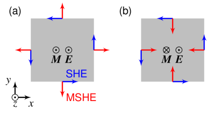
Figure 1: Conventional and magnetic spin Hall effect in ferromagnets with magnetization $\boldsymbol{M}$ along (a) $z$ direction and (b) $-z$ direction (e. g., MLG $4/mm^{\prime}m^{\prime}$). Upon application of an electric field $\boldsymbol{E}$ in $z$ direction (and a charge current in the same direction) spin accumulates at the boundaries of the sample. Those associated with the conventional spin Hall effect (SHE) are indicated by blue arrows, those with the MSHE by red arrows. Magnetization reversal acts only on the MSHE accumulations.

To elaborate on the difference to the SHE, let us assume that an electric field $\boldsymbol{E}\parallel\boldsymbol{M}\parallel\hat{\boldsymbol{z}}$ is applied, as depicted in Fig. 1. Due to the (conventional) SHE spin conductivity tensor elements ($\sigma^{x}_{yz}=-\sigma^{y}_{xz}$) spin is accumulated within the surface planes of the sample (blue arrows). The polarization of these spin accumulations is orthogonal to both $\boldsymbol{E}$ and the surface normal. Being time-reversal even, it does not flip under magnetization reversal [compare panel (a) vs. (b)]. In contrast, the MSHE ($\sigma^{x}_{xz}=\sigma^{y}_{yz}$) causes additional accumulations polarized normal to the surface planes (red arrows). Their time-reversal odd nature forces a flip upon magnetization reversal, as is represented by the reversed red arrows in panel (b).

Thus, the MSHE allows to generate a spin accumulation orthogonal to the conventional SHE spin accumulation. In scenarios in which the magnetization of the ferromagnet is fixed this feature may result in the decisive spin accumulation direction necessary to perform a particular spin torque switching. For example, the field-free magnetization switching of a perpendicularly magnetized film observed in Ref. Baek et al., 2018 may be explained in terms of MSHE spin accumulations. We emphasize that the existence of spin current vortices is a bulk property that gives rise to bulk MSHE spin currents, which, in turn, cause spin accumulations at the edges or interfaces. Additional interface effects, as those accounted for in Refs. Amin et al., 2018, Baek et al., 2018, and Hönemann et al., 2019, come on top.

That the SHE and MSHE cause spin accumulations pointing in orthogonal directions is a speciality of the MLGs $4/mm^{\prime}m^{\prime}$, $4^{\prime}/mm^{\prime}m$, and $m^{\prime}m^{\prime}m$, which allow for the ‘clearest’ disentanglement of MSHE and SHE. For other MLGs there is at least one element of the spin conductivity tensor that carries simultaneously contributions from the SHE and the MSHE, leaving the behavior under time-reversal (texture reversal) as the only distinguishing characteristic.

Apart from three-dimensional ferromagnets, two-dimensional electron gases (2DEGs) appear highly attractive. 2DEGs are well known for their efficient charge-to-spin conversion due to large Rashba SOC Lesne et al. (2016), magnetism in combination with superconductivity Brinkman et al. (2007); Reyren et al. (2007); Bert et al. (2011); Dikin et al. (2011); Li et al. (2011); Joshua et al. (2012), and electrical controllability Caviglia et al. (2008). Recent progress in achieving room temperature magnetism in 2DEGs Zhang et al. (2018b) suggests to investigate the MSHE in these systems. To do so we consider a minimal Rashba Hamiltonian with warping and an exchange field whose direction provides a handle to switch between different MLGs. It turns out that upon in-plane rotation of the field, the MSHE of in-plane polarized spins is manipulated but also that of out-of-plane polarized spins. Similar conclusions hold for topological Dirac surface states, as in Sn-doped Bi₂Te₃ Fu (2009) (e. g., in the presence of exchange fields due to proximity to a ferromagnetic normal insulator Eremeev et al. (2013)), and for the noncollinear antiferromagnet Mn₃Sn.

Instead of an electric field, a temperature gradient may be utilized to cause thermodynamic non-equilibrium and spin transport. As above for the SHE and the MSHE, time-reversal even transverse spin transport is then referred to as spin Nernst effect (SNE), and the time-reversal odd partner is termed magnetic SNE (MSNE). Since the spin current vortices in reciprocal space exist irrespective of the driving force, the existence of an MSHE immediately implies that of an MSNE. Recalling that the symmetry analysis is independent of the type of spin carriers, it applies just as well to magnetic insulators, in which spin is transported by magnons. We present a proof of principle by considering antiferromagnetic spin textures, as in Mn₃Sn, and demonstrate that the magnetic excitations give rise to nonzero spin current vortices and, thus, to a magnonic MSNE. Therefore, the results of this Paper can be carried over to the realm of spincaloritronics in magnetic insulators, where they may inspire studies of novel heat-to-spin conversion mechanisms and energy harvesting concepts.

The remainder of the Paper is organized as follows. In Sec. III the theoretical framework within which we describe spin transport is introduced. We disentangle time-reversal even from odd contributions in Sec. III.1, isolate the MSHE and introduce the SCV interpretation in Sec. III.2. Then, we turn to the symmetry analysis of all MLGs and summarize key findings in Sec. III.3. These are elaborated on in Sec. IV by considering specific toy models; the latter serve to underline the minimal requirements for a nonzero MSHE (Sec. IV.1), to make connection to magnetized Rashba materials (Sec. IV.2, and to demonstrate the magnonic MSNE (Sec. IV.3). We discuss the relation of our work to literature in Sec. V and summarize in Sec. VI.

III Linear-response theory of the magnetic spin Hall effect

The elements of the optical spin conductivity tensor read Seemann et al. (2015)

$$\sigma^{\gamma}_{\mu\nu}(\varpi)=\frac{1}{V}\int_{0}^{\infty}\mathrm{d}t\,\mathrm{e}^{\mathrm{i}\varpi t}\int_{0}^{\beta}\mathrm{d}\kappa\left\langle J_{\nu}J^{\gamma}_{\mu}(t+\mathrm{i}\hbar\kappa)\right\rangle$$ (3)

in Kubo linear-response theory Kubo et al. (1957); Mahan (2000). $J_{\nu}$, $J^{\gamma}_{\mu}$, $\varpi$, $V$, and $\beta$ are the total charge and spin current operators, the frequency of $\boldsymbol{E}(\varpi)$, the system’s volume, and the inverse temperature, respectively. The shape of $\underline{\sigma}^{\gamma}$ was derived for all MLGs by symmetry arguments in Ref. Seemann et al., 2015. However, such a superordinate symmetry approach neither provides insights into the character of the MSHE nor does it identify the MSHE contributions to the tensor elements. The latter requires to decompose $\underline{\sigma}^{\gamma}$.

III.1 Decomposition of the spin conductivity tensor

We work in the limit of non-interacting electrons described by the Hamiltonian

$$H=\sum_{\boldsymbol{k}}\boldsymbol{\varPsi}^{\dagger}_{\boldsymbol{k}}\underline{H}_{\boldsymbol{k}}\boldsymbol{\varPsi}_{\boldsymbol{k}}$$ (4)

in crystal momentum ($\boldsymbol{k}$) representation. $\boldsymbol{\varPsi}^{\dagger}_{\boldsymbol{k}}$ ($\boldsymbol{\varPsi}_{\boldsymbol{k}}$) is a vector of electronic creation (annihilation) operators; its index runs over spin, orbitals, and basis lattice sites. The eigenenergies $\varepsilon_{n\boldsymbol{k}}$ and corresponding eigenvectors $|n\rangle=|u_{n\boldsymbol{k}}\rangle$, which represent the lattice-periodic part of a Bloch wavefunction with band index $n$, are obtained from diagonalizing the Hamilton kernel $\underline{H}_{\boldsymbol{k}}$.

The dc spin conductivity then reads

$$\sigma^{\gamma}_{\mu\nu}\equiv\mathrm{Re}\left[\lim_{\varpi\to 0}\sigma^{\gamma}_{\mu\nu}(\varpi)\right]=\sigma^{\gamma,\mathrm{odd}}_{\mu\nu}+\sigma^{\gamma,\mathrm{even}}_{\mu\nu},$$ (5)

with the two contributions Železný et al. (2017)

$$\sigma^{\gamma,\mathrm{odd}}_{\mu\nu} =\frac{\hbar^{2}\varGamma}{V}\sum_{n,m,\boldsymbol{k}}\frac{f_{m\boldsymbol{k}}-f_{n\boldsymbol{k}}}{\varepsilon_{n\boldsymbol{k}}-\varepsilon_{m\boldsymbol{k}}}\frac{\mathrm{Re}\left(\langle n|\underline{J}^{\gamma}_{\boldsymbol{k},\mu}|m\rangle\langle m|\underline{J}_{\boldsymbol{k},\nu}|n\rangle\right)}{\left(\varepsilon_{n\boldsymbol{k}}-\varepsilon_{m\boldsymbol{k}}\right)^{2}+\left(\hbar\varGamma\right)^{2}},$$ (6a)

$$\sigma^{\gamma,\mathrm{even}}_{\mu\nu} =-\frac{\hbar}{V}\sum_{n,m,\boldsymbol{k}}\left(f_{m\boldsymbol{k}}-f_{n\boldsymbol{k}}\right)\frac{\mathrm{Im}\left(\langle n|\underline{J}^{\gamma}_{\boldsymbol{k},\mu}|m\rangle\langle m|\underline{J}_{\boldsymbol{k},\nu}|n\rangle\right)}{\left(\varepsilon_{n\boldsymbol{k}}-\varepsilon_{m\boldsymbol{k}}\right)^{2}+\left(\hbar\varGamma\right)^{2}}.$$ (6b)

$f_{n\boldsymbol{k}}=(\mathrm{e}^{\beta(\varepsilon_{n\boldsymbol{k}}-\varepsilon_{\mathrm{F}})}+1)^{-1}$ is the Fermi distribution function with Fermi energy $\varepsilon_{\mathrm{F}}$. $\hbar\varGamma$ is an artificial spectral broadening and the total currents are decomposed into their Fourier kernels $\underline{J}^{\gamma}_{\boldsymbol{k},\mu}$ and $\underline{J}_{\boldsymbol{k},\nu}=-e\underline{v}_{\boldsymbol{k},\nu}=-e\hbar^{-1}\partial\underline{H}_{\boldsymbol{k}}/\partial k_{\nu}$ (in the $\boldsymbol{\varPsi}_{\boldsymbol{k}}$ basis), respectively.

The superscripts of $\sigma^{\gamma,\mathrm{odd}}_{\mu\nu}$ and $\sigma^{\gamma,\mathrm{even}}_{\mu\nu}$ indicate their behavior under time-reversal. We recall that spin (charge) current is time-reversal even (odd) and that the TR operator comprises complex conjugation Železný et al. (2017). The behavior under time reversal can be addressed by a reversal of the magnetic texture (a collection $\{\boldsymbol{m}_{i}\}$ of magnetic moments):

$$\sigma^{\gamma,\mathrm{odd}}_{\mu\nu}[\{\boldsymbol{m}_{i}\}] =-\sigma^{\gamma,\mathrm{odd}}_{\mu\nu}[-\{\boldsymbol{m}_{i}\}],$$ (7)

$$\sigma^{\gamma,\mathrm{even}}_{\mu\nu}[\{\boldsymbol{m}_{i}\}] =\sigma^{\gamma,\mathrm{even}}_{\mu\nu}[-\{\boldsymbol{m}_{i}\}].$$

In an experiment these contributions can be disentangled by measuring the spin accumulations brought about by the spin currents for both the original and the reversed texture.

Following up on Eq. (6a), a MSHE was identified by symmetry arguments for Mn${}_{3}X$ ($X=\mathrm{Sn,Ga,Ge}$) in Ref. Železný et al., 2017 (see the first entry in the right column of Tab. I of that paper and consider $\sigma^{x}_{xy}\neq\sigma^{x}_{yx}$, which makes the antisymmetric part of $\underline{\sigma}^{x}$ nonzero). The term MSHE was coined in Refs. Chen et al., 2018; Kimata et al., 2019, the latter of which reported on its experimental observation in Mn₃Sn.

In what follows we concentrate on $\sigma^{\gamma,\mathrm{odd}}_{\mu\nu}$, because $\sigma^{\gamma,\mathrm{even}}_{\mu\nu}$ is related to the intrinsic SHE Sinova et al. (2004) which is of minor interest in this Paper. We decompose $\sigma^{\gamma,\mathrm{odd}}_{\mu\nu}$ into intraband contributions ($n=m$)

$$\sigma^{\gamma,\mathrm{odd}}_{\mu\nu,\mathrm{intra}} =\frac{1}{\varGamma V}\sum_{n,\boldsymbol{k}}J^{\gamma}_{n\boldsymbol{k},\mu}J_{n\boldsymbol{k},\nu}\left(-\frac{\partial f_{n\boldsymbol{k}}}{\partial\varepsilon}\right)$$ (8)

and interband contributions given by Eq. (6a) with the sum restricted to $n\neq m$. $J^{\gamma}_{n\boldsymbol{k},\mu}\equiv\langle n|\underline{J}^{\gamma}_{\boldsymbol{k},\mu}|n\rangle$ is the spin and $J_{n\boldsymbol{k},\nu}\equiv-e\langle n|\underline{v}_{\boldsymbol{k},\nu}|n\rangle=-ev_{n\boldsymbol{k},\nu}$ the charge current expectation value; $v_{n\boldsymbol{k},\nu}=\hbar^{-1}\partial\varepsilon_{n\boldsymbol{k}}/\partial k_{\nu}$ is the group velocity and $e>0$ the elementary charge. We note in passing that Eq. (8) can also be derived within the semiclassical Boltzmann transport theory, assuming a constant relaxation time. For $\varGamma\to 0$, $\sigma^{\gamma,\mathrm{odd}}_{\mu\nu,\mathrm{intra}}$ diverges while the interband contributions converge to a constant. From here on, we thus drop the specifiers ‘odd’ and ‘intra’, work in the ‘almost clean’ limit ($\hbar\varGamma>0$ is the smallest energy scale), and focus on the dominating intraband contribution in Eq. (8).

III.2 Identification of the MSHE contributions

The antisymmetric part

$$\underline{\sigma}^{\gamma,\mathrm{(a)}}\equiv\frac{\underline{\sigma}^{\gamma}-\underline{\sigma}^{\gamma,\mathrm{T}}}{2}$$ (9)

of the time-odd spin conductivity tensor describes the MSHE. Since any antisymmetric matrix can be represented by a vector, we introduce the $\gamma$-spin MSHE vector as $[\boldsymbol{\sigma}^{\gamma}_{\mathrm{MSHE}}]_{\times}=\underline{\sigma}^{\gamma,\mathrm{(a)}}$, written compactly as [cf. eq. (8)]

$$\boldsymbol{\sigma}^{\gamma}_{\mathrm{MSHE}}\equiv\begin{pmatrix}\sigma^{\gamma,\mathrm{(a)}}_{yz}\\ \sigma^{\gamma,\mathrm{(a)}}_{zx}\\ \sigma^{\gamma,\mathrm{(a)}}_{xy}\end{pmatrix}=\frac{1}{2\varGamma V}\sum_{n,\boldsymbol{k}}\boldsymbol{J}^{\gamma}_{n\boldsymbol{k}}\times\boldsymbol{J}_{n\boldsymbol{k}}\left(-\frac{\partial f_{n\boldsymbol{k}}}{\partial\varepsilon}\right).$$ (10)

At zero temperature, $-\partial f_{n\boldsymbol{k}}/\partial\varepsilon=\delta(\varepsilon_{n\boldsymbol{k}}-\varepsilon_{\mathrm{F}})$ allows to replace the $\boldsymbol{k}$ summation by an integral over the Fermi surface,

$$\boldsymbol{\sigma}^{\gamma}_{\mathrm{MSHE}}=\frac{e}{2\hbar\varGamma(2\pi)^{3}}\sum_{n}\oint_{\varepsilon_{n}=\varepsilon_{\mathrm{F}}}\hat{\boldsymbol{v}}_{n\boldsymbol{k}}\times\boldsymbol{J}^{\gamma}_{n\boldsymbol{k}}\,\mathrm{d}S$$ (11)

($\hat{\boldsymbol{v}}_{n\boldsymbol{k}}=\boldsymbol{v}_{n\boldsymbol{k}}/v_{n\boldsymbol{k}}$ is the local normal of the Fermi surface). This integral measures the tangential vector flow of $\boldsymbol{J}^{\gamma}_{n\boldsymbol{k}}$ on the Fermi surface. $\boldsymbol{\sigma}^{\gamma}_{\mathrm{MSHE}}$ is nonzero if there is an integrated sense of rotation of the spin current about the Fermi surface.

Alternatively, we write Eq. (11) as a Fermi sea integral,

$$\boldsymbol{\sigma}^{\gamma}_{\mathrm{MSHE}}=\frac{e}{2\hbar\varGamma(2\pi)^{3}}\boldsymbol{\omega}^{\gamma}(\varepsilon_{\mathrm{F}}),$$ (12)

over the net spin current vorticity (SCV)

$$\boldsymbol{\omega}^{\gamma}(\varepsilon_{\mathrm{F}})\equiv\sum_{n}\iiint_{\varepsilon_{n}\leq\varepsilon_{\mathrm{F}}}\boldsymbol{\omega}^{\gamma}_{n\boldsymbol{k}}\,\mathrm{d}^{3}k,\quad\boldsymbol{\omega}^{\gamma}_{n\boldsymbol{k}}\equiv\boldsymbol{\nabla}_{\boldsymbol{k}}\times\boldsymbol{J}^{\gamma}_{n\boldsymbol{k}},$$ (13)

that is defined in analogy to the vorticity of a fluid Landau and Lifshitz (2013). $\boldsymbol{\omega}^{\gamma}_{n\boldsymbol{k}}$ describes the local rotation, shear or curvature of $\boldsymbol{J}^{\gamma}_{n\boldsymbol{k}}$. Figuratively speaking, the vorticity of a vector field is nonzero at those points at which a paddle wheel would start to rotate (note that integrals over fully occupied bands are zero, i. e., each band has a vanishing total SCV).

Equations (11) – (13) are our main findings. They show that a MSHE is a result of the spin current circulation about the Fermi surface [Eq. (11)] or, put differently, a result of a finite SCV in the Fermi sea [Eq. (12)].

For illustration we stretch the analogy to fluid vortices and recall the time-reversal asymmetric propagation of an acoustic wave through a fluid with a vortex Roux and Fink (1995), briefly laid out in the introduction. The broken TRS in magnets causes SCVs $\boldsymbol{\omega}^{\gamma}$ for each spin component $\gamma=x,y,z$ in the Fermi sea, which is experienced by the $\gamma$ spin component of an electron’s Bloch wave propagating through the crystal. A consequence is a Hall-like deflection within the plane normal to $\boldsymbol{\omega}^{\gamma}$ of that spin component. Time reversal is equivalent to inversion of the vortex’s circulation direction ($\boldsymbol{\omega}^{\gamma}\to-\boldsymbol{\omega}^{\gamma}$), which signifies the time-odd signature of the MSHE.

Considering reciprocal space, a simple picture may be helpful. In a two-dimensional crystal with a single Fermi line, the spin current vector field $\boldsymbol{J}^{\gamma}_{\boldsymbol{k}}$ may look as depicted in Fig. 2 (we suppressed the band index). The integral of the $\boldsymbol{k}$-dependent vorticity over the Fermi sea is proportional to the magnetic spin Hall conductivity. In scenario (a), $\boldsymbol{J}^{\gamma}_{\boldsymbol{k}}$ is irrotational and, thus, has zero vorticity. In (b) $\boldsymbol{J}^{\gamma}_{\boldsymbol{k}}$ shows local vorticity that integrates to zero due to symmetry. And in (c), the Fermi surface cuts out a region with nonzero vorticity causing a MSHE. To check the behavior under time reversal recall the mapping $\boldsymbol{J}^{\gamma}_{\boldsymbol{k}}$ to $\boldsymbol{J}^{\gamma}_{-\boldsymbol{k}}$, which reverses the circulation direction.

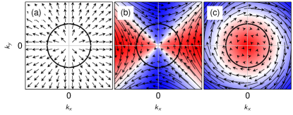
Figure 2: Vorticities of spin current vector fields in reciprocal space. Red/white/blue color indicates positive/zero/blue vorticity in a region about the origin. The integral over the vorticity within the Fermi surface, indicated by black circles, is proportional to the magnetic spin Hall conductivity. (a) The irrotational source field has zero vorticity. (b) The quadrupolar field has locally nonzero vorticity but zero integral. (c) A general vortex with vorticity of varying sign.

One may discuss the effect in terms of a shift of the Fermi surface that is caused by the redistribution of electrons. An electric field $\boldsymbol{E}$ along $-x$ direction produces a shift in positive $k_{x}$ direction (accounting for the negative electron charge). For the situation in Fig. 2(a), this displacement does not yield a transversal response since $\langle\boldsymbol{j}^{\gamma}\rangle\parallel\hat{\boldsymbol{x}}$. However, for (b) and (c) $\langle\boldsymbol{j}^{\gamma}\rangle\parallel\hat{\boldsymbol{y}}$ and $\langle\boldsymbol{j}^{\gamma}\rangle\parallel-\hat{\boldsymbol{y}}$, respectively. If $\boldsymbol{E}$ is along the $-y$ direction (shift in positive $k_{y}$ direction), $\langle\boldsymbol{j}^{\gamma}\rangle\parallel\hat{\boldsymbol{x}}$ for both (b) and (c). Hence, only a finite SCV, as depicted in (c), fixes the sign of $\langle\boldsymbol{j}^{\gamma}\rangle\times\boldsymbol{E}$, thereby causing a nonzero antisymmetric part of $\underline{\sigma}^{\gamma}$, that is a MSHE. The scenario (b) gives rise to a symmetric part of $\underline{\sigma}^{\gamma}$, conceivably referred to as ‘planar magnetic spin Hall effect’.

III.3 Symmetry analysis

Although breaking of TRS is necessary for a nonzero local SCV $\boldsymbol{\omega}^{\gamma}_{n\boldsymbol{k}}$, it is not sufficient because symmetries of the magnetic crystal may render the SCV integral in Eq. (13) zero [cf. Fig. 2(b)]. In what follows we derive which MLGs do or do not allow for a MSHE. The restriction to MLGs—instead to magnetic point groups—is feasible because $\underline{\sigma}^{\gamma}$ is related to the correlation function of a spin current and a charge current [Eq. (3)]. Both currents change sign upon inversion; thus, the presence or absence of inversion symmetry does not impose restrictions on the shape of the spin conductivity tensor. One may then augment each magnetic point group with the element of space inversion to map it onto the set of MLGs. Recall that the considerably smaller number of MLGs facilitates the analysis. This argumentation is in line with Refs. Kleiner (1966, 1967, 1969); Seemann et al. (2015). We like to refer the reader to Ref. Seemann et al. (2015) for mappings of magnetic point groups onto MLGs.

We combine the three spin-dependent MSHE vectors of Eq. (12) to the MSHE tensor

$$\underline{\sigma}_{\mathrm{MSHE}}\equiv\left(\boldsymbol{\sigma}^{x}_{\mathrm{MSHE}},\boldsymbol{\sigma}^{y}_{\mathrm{MSHE}},\boldsymbol{\sigma}^{z}_{\mathrm{MSHE}}\right)\propto\underline{\omega}\equiv\left(\boldsymbol{\omega}^{x},\boldsymbol{\omega}^{y},\boldsymbol{\omega}^{z}\right).$$ (14)

Equation (14) links the elements of $\underline{\sigma}_{\mathrm{MSHE}}$ to those of the SCV tensor $\underline{\omega}$, the latter itself constructed from the three spin current vorticity vectors given in Eq. (13) (argument $\varepsilon_{\mathrm{F}}$ suppressed). $\underline{\omega}$ can be decomposed into three contributions:

$$\underline{\omega}=\omega\underline{I}+[\boldsymbol{\varOmega}]_{\times}+\underline{W},$$ (15)

that is a scalar $\omega=\operatorname{Tr}(\underline{\omega})/3$, a vector $[\boldsymbol{\varOmega}]_{\times}=(\underline{\omega}-\underline{\omega}^{\mathrm{T}})/2$, and a traceless symmetric tensor $\underline{W}=(\underline{\omega}+\underline{\omega}^{\mathrm{T}})/2-\omega\underline{I}$, with $\underline{I}$ the $3\times 3$ identity matrix. Recalling that $\underline{\omega}$ is time-reversal odd but space-inversion even and calling to mind the transformation properties of electromagnetic multipoles Nanz (2016), one finds that $\omega$, $\boldsymbol{\varOmega}$, and $\underline{W}$ transform as a magnetic toroidal monopole (Jahn symbol $a$, Ref. Jahn, 1949), a magnetic dipole ($eaV$), and a magnetic toroidal quadrupole ($a[V^{2}]$), respectively. Such a multipole decomposition is in line with Ref. Hayami et al., 2018 [cf. Eqs. (D20) and (D21) of that publication].

Utilizing the Mtensor application Gallego et al. (2019) of the Bilbao Crystallographic Server Aroyo et al. (2006a, b, 2011), we identified all MLGs permitting these multipoles. By virtue of Eqs. (10) and (14) these results are carried forward to $\underline{\sigma}_{\mathrm{MSHE}}$ and $\underline{\sigma}^{\gamma,\mathrm{(a)}}$; a summary is given in Table 1. The results of the symmetry analysis are not restricted to the intraband approximation (i. e., the interpretation in terms of SCVs) but apply to Eq. (6a) as well [one may consider the summand in Eq. (6a) as a generalization of the SCV to interband contributions]. We now list and discuss illustrative key findings.

Table 1: Symmetry analysis of the MSHE. The columns give magnetic Laue groups (MLGs), components of the spin current vorticity (SCV) $\underline{\omega}$, and elements of spin conductivity $\underline{\sigma}^{\gamma}$ that are compatible with an MSHE.

MLG	Admitted elements of SCV tensor $\underline{\omega}$			MSHE part of spin conductivity tensor $\underline{\sigma}^{\gamma}$
	$\omega$	$\boldsymbol{\varOmega}$	$\underline{W}$	$\underline{\sigma}^{x,\mathrm{(a)}}$	$\underline{\sigma}^{y,\mathrm{(a)}}$	$\underline{\sigma}^{z,\mathrm{(a)}}$
$\bar{1}$	$\omega$	$\varOmega_{x}$, $\varOmega_{y}$, $\varOmega_{z}$	$W_{x}^{x}$, $W_{y}^{y}$, $W_{z}^{z}$, $W_{x}^{y}$, $W_{x}^{z}$, $W_{y}^{z}$	$\begin{pmatrix}0&\sigma^{x}_{xy}&\sigma^{x}_{xz}\\ -\sigma^{x}_{xy}&0&\sigma_{yz}^{x}\\ -\sigma^{x}_{xz}&-\sigma_{yz}^{x}&0\end{pmatrix}$	$\begin{pmatrix}0&\sigma^{y}_{xy}&\sigma_{xz}^{y}\\ -\sigma^{y}_{xy}&0&\sigma^{y}_{yz}\\ -\sigma_{xz}^{y}&-\sigma^{y}_{yz}&0\end{pmatrix}$	$\begin{pmatrix}0&\sigma_{xy}^{z}&\sigma^{z}_{xz}\\ -\sigma_{xy}^{z}&0&\sigma^{z}_{yz}\\ -\sigma^{z}_{xz}&-\sigma^{z}_{yz}&0\end{pmatrix}$
$2/m$	$\omega$	$\varOmega_{y}$	$W_{x}^{x}$, $W_{y}^{y}$, $W_{z}^{z}$, $W_{x}^{z}$	$\begin{pmatrix}0&\sigma^{x}_{xy}&0\\ -\sigma^{x}_{xy}&0&\sigma_{yz}^{x}\\ 0&-\sigma_{yz}^{x}&0\end{pmatrix}$	$\begin{pmatrix}0&0&\sigma_{xz}^{y}\\ 0&0&0\\ -\sigma_{xz}^{y}&0&0\end{pmatrix}$	$\begin{pmatrix}0&\sigma_{xy}^{z}&0\\ -\sigma_{xy}^{z}&0&\sigma^{z}_{yz}\\ 0&-\sigma^{z}_{yz}&0\end{pmatrix}$
$mmm$	$\omega$	$-$	$W_{x}^{x}$, $W_{y}^{y}$, $W_{z}^{z}$	$\begin{pmatrix}0&0&0\\ 0&0&\sigma_{yz}^{x}\\ 0&-\sigma_{yz}^{x}&0\end{pmatrix}$	$\begin{pmatrix}0&0&\sigma_{xz}^{y}\\ 0&0&0\\ -\sigma_{xz}^{y}&0&0\end{pmatrix}$	$\begin{pmatrix}0&\sigma_{xy}^{z}&0\\ -\sigma_{xy}^{z}&0&0\\ 0&0&0\end{pmatrix}$
$4/m$	$\omega$	$\varOmega_{z}$	$W_{x}^{x}=W_{y}^{y}$, $W_{z}^{z}$	$\begin{pmatrix}0&0&\sigma_{xz}^{x}\\ 0&0&\sigma_{yz}^{x}\\ -\sigma_{xz}^{x}&-\sigma_{yz}^{x}&0\end{pmatrix}$	$\begin{pmatrix}0&0&-\sigma_{yz}^{x}\\ 0&0&\sigma_{xz}^{x}\\ \sigma_{yz}^{x}&-\sigma_{xz}^{x}&0\end{pmatrix}$	$\begin{pmatrix}0&\sigma_{xy}^{z}&0\\ -\sigma_{xy}^{z}&0&0\\ 0&0&0\end{pmatrix}$
$6/m$
$\bar{3}$
$4/mmm$	$\omega$	$-$	$W_{x}^{x}=W_{y}^{y}$, $W_{z}^{z}$	$\begin{pmatrix}0&0&0\\ 0&0&\sigma_{yz}^{x}\\ 0&-\sigma_{yz}^{x}&0\end{pmatrix}$	$\begin{pmatrix}0&0&-\sigma_{yz}^{x}\\ 0&0&0\\ \sigma_{yz}^{x}&0&0\end{pmatrix}$	$\begin{pmatrix}0&\sigma_{xy}^{z}&0\\ -\sigma_{xy}^{z}&0&0\\ 0&0&0\end{pmatrix}$
$6/mmm$
$\bar{3}m$
$m\bar{3}$	$\omega$	$-$	$W_{x}^{x}=W_{y}^{y}=W_{z}^{z}$	$\begin{pmatrix}0&0&0\\ 0&0&\sigma_{yz}^{x}\\ 0&-\sigma_{yz}^{x}&0\end{pmatrix}$	$\begin{pmatrix}0&0&-\sigma_{yz}^{x}\\ 0&0&0\\ \sigma_{yz}^{x}&0&0\end{pmatrix}$	$\begin{pmatrix}0&\sigma_{yz}^{x}&0\\ -\sigma_{yz}^{x}&0&0\\ 0&0&0\end{pmatrix}$
$m\bar{3}m$
$2^{\prime}/m^{\prime}$	$-$	$\varOmega_{x}$, $\varOmega_{z}$	$W_{x}^{y}$, $W_{y}^{z}$	$\begin{pmatrix}0&0&\sigma_{xz}^{x}\\ 0&0&0\\ -\sigma_{xz}^{x}&0&0\end{pmatrix}$	$\begin{pmatrix}0&\sigma_{xy}^{y}&0\\ -\sigma_{xy}^{y}&0&\sigma_{yz}^{y}\\ 0&-\sigma_{yz}^{y}&0\end{pmatrix}$	$\begin{pmatrix}0&0&\sigma_{xz}^{z}\\ 0&0&0\\ -\sigma_{xz}^{z}&0&0\end{pmatrix}$
$m^{\prime}m^{\prime}m$	$-$	$\varOmega_{z}$	$W_{x}^{y}$	$\begin{pmatrix}0&0&\sigma_{xz}^{x}\\ 0&0&0\\ -\sigma_{xz}^{x}&0&0\end{pmatrix}$	$\begin{pmatrix}0&0&0\\ 0&0&\sigma_{yz}^{y}\\ 0&-\sigma_{yz}^{y}&0\end{pmatrix}$	$-$
$4^{\prime}/m$	$-$	$-$	$W_{x}^{y}$, $W_{x}^{x}=-W_{y}^{y}$	$\begin{pmatrix}0&0&\sigma_{xz}^{x}\\ 0&0&\sigma_{yz}^{x}\\ -\sigma_{xz}^{x}&-\sigma_{yz}^{x}&0\end{pmatrix}$	$\begin{pmatrix}0&0&\sigma_{yz}^{x}\\ 0&0&-\sigma_{xz}^{x}\\ -\sigma_{yz}^{x}&\sigma_{xz}^{x}&0\end{pmatrix}$	$-$
$4^{\prime}/mm^{\prime}m$	$-$	$-$	$W_{x}^{y}$	$\begin{pmatrix}0&0&\sigma_{xz}^{x}\\ 0&0&0\\ -\sigma_{xz}^{x}&0&0\end{pmatrix}$	$\begin{pmatrix}0&0&0\\ 0&0&-\sigma_{xz}^{x}\\ 0&\sigma_{xz}^{x}&0\end{pmatrix}$	$-$
$4/mm^{\prime}m^{\prime}$	$-$	$\varOmega_{z}$	$-$	$\begin{pmatrix}0&0&\sigma_{xz}^{x}\\ 0&0&0\\ -\sigma_{xz}^{x}&0&0\end{pmatrix}$	$\begin{pmatrix}0&0&0\\ 0&0&\sigma_{xz}^{x}\\ 0&-\sigma_{xz}^{x}&0\end{pmatrix}$	$-$
$6/mm^{\prime}m^{\prime}$
$\bar{3}m^{\prime}$

(i) Any MLG that contains pure time-reversal $1^{\prime}$ (reversal of the magnetic texture maps the crystal onto itself modulo a translation) is incompatible with a SCV and a MSHE because $\omega$, $\boldsymbol{\varOmega}$, and $\underline{W}$ transform as magnetic multipoles.

(ii) The MLG $m\bar{3}m$ of cubic systems does not allow for a magnetization ($\boldsymbol{\varOmega}=\boldsymbol{0}$) but for $\omega$ and $W_{x}^{x}=W_{y}^{y}=W_{z}^{z}$, from which

$$\stackrel{{\scriptstyle\mathrm{Eq.~{}\eqref{eq:vorticity-decomp}}}}{{\to}}\omega_{x}^{x}=\omega_{y}^{y}=\omega_{z}^{z} \stackrel{{\scriptstyle\mathrm{Eq.~{}\eqref{eq:connectionMSHEvorticity}}}}{{\to}}\sigma_{\mathrm{MSHE},x}^{x}=\sigma_{\mathrm{MSHE},y}^{y}=\sigma_{\mathrm{MSHE},z}^{z}$$

$$\stackrel{{\scriptstyle\mathrm{Eq.~{}\eqref{eq:MSHEvector}}}}{{\to}}\sigma^{x,\mathrm{(a)}}_{yz}=\sigma^{y,\mathrm{(a)}}_{zx}=\sigma^{z,\mathrm{(a)}}_{xy}$$

follows. MSHEs with mutually orthogonal spin, flow, and force directions are expected, a situation known from the SHE in nonmagnetic cubic materials. The SHE and MSHE can be disentangled by their opposite time-reversal signature which can be probed by a reversal of the magnetic texture Kimata et al. (2019).

(iii) The MLG $4/mm^{\prime}m^{\prime}$ admits of a magnetization, $\boldsymbol{\varOmega}=(0,0,\varOmega_{z})^{\mathrm{T}}$, but neither of $\omega$ nor of $\underline{W}$. We find

$$W_{x}^{y}=0,\;\varOmega_{z}\neq 0 \stackrel{{\scriptstyle\mathrm{Eq.~{}\eqref{eq:vorticity-decomp}}}}{{\to}}\omega_{x}^{y}=-\omega_{y}^{x}\stackrel{{\scriptstyle\mathrm{Eq.~{}\eqref{eq:connectionMSHEvorticity},\eqref{eq:MSHEvector}}}}{{\to}}\sigma^{y,\mathrm{(a)}}_{yz}=-\sigma^{x,\mathrm{(a)}}_{zx}.$$

In contrast to the anomalous Hall effect (AHE), a magnetization (along $z$) does not cause transverse transport within a plane perpendicular to it ($xy$ plane), but in planes that contain itself ($xz$ and $yz$ planes). Only the transported spin component has to be normal to the magnetization ($x$ and $y$). Moreover, it has to lie within the plane of transport. Thus, although tetragonal ferromagnets allow both for the AHE and the MSHE, the spin current attributed to the MSHE is a pure spin current because the AHE-induced current flows in a different plane. This scenario was outlined in Sec. II via Eq. (2).

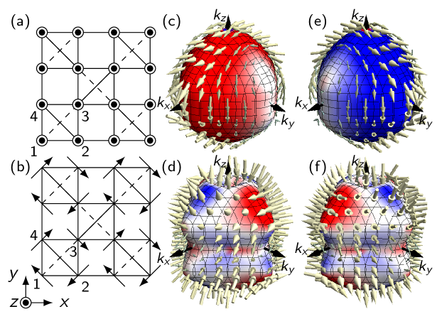
Figure 3: MSHE in the pyrochlore lattice for (a) ferromagnetic (MLG $4/mm^{\prime}m^{\prime}$) and (b) antiferromagnetic textures (MLG $4^{\prime}/mm^{\prime}m$). The pyrochlore lattice is projected onto the $xy$ plane, such that the tetrahedra appear as squares. (c) and (d) depict Fermi surfaces with arrows indicating $\boldsymbol{J}^{x}_{\boldsymbol{k}}$ and the color scale depicts the $y$ component of $\hat{\boldsymbol{v}}_{\boldsymbol{k}}\times\boldsymbol{J}^{x}_{\boldsymbol{k}}$ (blue/white/red indicates negative/zero/positive values; the value range is symmetric about zero). (e) and (f) as (c) and (d) but for $\boldsymbol{J}^{y}_{\boldsymbol{k}}$ and the $x$ component of $\hat{\boldsymbol{v}}_{\boldsymbol{k}}\times\boldsymbol{J}^{y}_{\boldsymbol{k}}$.

(iv) A magnetic toroidal quadrupole $\underline{W}$ also allows for the spin transport discussed in (iii). Consider the MLG $4^{\prime}/mm^{\prime}m$ that permits only a nonzero $W_{x}^{y}$, which translates to $\sigma^{y,\mathrm{(a)}}_{yz}=\sigma^{x,\mathrm{(a)}}_{zx}$. Compared to (iii), only the relation of the signs of nonzero components has changed. For a geometry as depicted in Fig. 1 (four-fold rotational axis aligned with the $z$ direction), this reversed sign translates into a MSHE spin accumulation with a polarization that alternates between pointing parallel and antiparallel to the surface normal.

(v) The MLG $m^{\prime}m^{\prime}m$ combines the scenarios of (iii) and (iv): $\varOmega_{z}$, $W_{x}^{y}$, $\sigma^{y,\mathrm{(a)}}_{yz}$, and $\sigma^{x,\mathrm{(a)}}_{zx}$ may be nonzero but there is no additional symmetry-imposed relation between the latter two.

(vi) An MSHE has been experimentally established in the noncollinear antiferromagnet Mn₃Sn Kimata et al. (2019) that—depending on the spin orientation—belongs either to the MLG $2^{\prime}/m^{\prime}$ or to $2/m$ . These are the same MLGs we shall discuss in the context of a magnetized Rashba electron gas with warping (Sec. IV.2). Please note that the MLG $2/m$ allows for $\sigma_{xy}^{z}\not=0$, that is a MSHE in the $xy$ plane with out-of-plane polarized spins currents (a geometry similar to the conventional SHE), whereas $2^{\prime}/m^{\prime}$ does not. Thus, upon rotation of the coplanar magnetic texture of Mn₃Sn, one could switch the MLGs and thereby engineer the transport of out-of-plane polarized spins; this effect awaits experimental verification (the experimental setup in Ref. Kimata et al., 2019 was sensitive to in-plane spin polarizations).

IV Examples

With the above results at hand, we now address selected examples for various MLGs. Section IV.1 focuses on minimal requirements for a MSHE and illustrates its interpretation in terms of spin current vorticities. In Sec. IV.2 we make contact with Rashba materials whose MLGs cover Mn₃Sn. Finally, we consider a magnetic spin Nernst effect in insulating materials (Sec. IV.3).

IV.1 Minimal requirements for a MSHE

According to the points (iii) and (iv) in Section III.3, compatibility of a MLG with either a magnetization (e. g., MLG $4/mm^{\prime}m^{\prime}$) or a magnetic toroidal quadrupole (e. g., MLG $4^{\prime}/mm^{\prime}m$) suffices for a MSHE. To show explicitly the spin current vortex about the Fermi surface [in the sense of Eq. (11)], we consider the $sd$ Hamiltonian

$$H=\sum_{\langle ij\rangle}\boldsymbol{c}_{i}^{\dagger}\left(t+\mathrm{i}\alpha\boldsymbol{\tau}\cdot\hat{\boldsymbol{d}}_{ij}\right)\boldsymbol{c}_{j}+J\sum_{i}\boldsymbol{c}_{i}^{\dagger}\left(\boldsymbol{\tau}\cdot\hat{\boldsymbol{m}}_{i}\right)\boldsymbol{c}_{i}$$ (16)

on the pyrochlore lattice [Fig. 3(a)] which consists of corner-sharing tetrahedra Bzdušek et al. (2015). $\boldsymbol{c}^{\dagger}_{i}$ ($\boldsymbol{c}_{i}$) creates (annihilates) an electron spinor at site $i$, $\boldsymbol{\tau}^{\mathrm{T}}=(\underline{\tau}^{x},\underline{\tau}^{y},\underline{\tau}^{z})$ is the vector of Pauli matrices. The hopping (with amplitude $t$) of electrons is accompanied by a spin rotation due to SOC (with amplitude $\alpha$). The unit vectors

$$\hat{\boldsymbol{d}}_{12}=\frac{\sqrt{2}}{2}\begin{pmatrix}-1\\ 0\\ 1\end{pmatrix},\quad\hat{\boldsymbol{d}}_{13}=\frac{\sqrt{2}}{2}\begin{pmatrix}1\\ -1\\ 0\end{pmatrix},\quad\hat{\boldsymbol{d}}_{14}=\frac{\sqrt{2}}{2}\begin{pmatrix}0\\ 1\\ -1\end{pmatrix},$$ (17)

$$\hat{\boldsymbol{d}}_{23}=\frac{\sqrt{2}}{2}\begin{pmatrix}0\\ 1\\ 1\end{pmatrix},\quad\hat{\boldsymbol{d}}_{24}=\frac{\sqrt{2}}{2}\begin{pmatrix}-1\\ -1\\ 0\end{pmatrix},\quad\hat{\boldsymbol{d}}_{34}=\frac{\sqrt{2}}{2}\begin{pmatrix}1\\ 0\\ 1\end{pmatrix}$$

specify the directions of the effective SOC. Each of the $\hat{\boldsymbol{d}}_{ij}$ is orthogonal to the $i$–$j$ bond and lies within a face of a cube that encloses a tetrahedron. $\hat{\boldsymbol{d}}_{ij}=-\hat{\boldsymbol{d}}_{ji}$ implies $\sum_{j=1}^{4}\hat{\boldsymbol{d}}_{ij}=\boldsymbol{0}$ for each $i=1,\ldots,4$.

Via Hund’s coupling $J$, the electron spins are connected with the local magnetic moments $\hat{\boldsymbol{m}}_{i}$ (black arrows in Fig. 3). The ferromagnetic texture in (a), with $\hat{\boldsymbol{m}}_{i}=(0,0,1)^{\mathrm{T}}$, belongs to the MLG $4/mm^{\prime}m^{\prime}$, while the antiferromagnetic texture in (b) belongs to $4^{\prime}/mm^{\prime}m$ (the notation of the MLGs matches that of the respective magnetic point groups):

$$\hat{\boldsymbol{m}}_{1}=\frac{\sqrt{2}}{2}\begin{pmatrix}-1\\ 1\\ 0\end{pmatrix},\quad\hat{\boldsymbol{m}}_{2}=\frac{\sqrt{2}}{2}\begin{pmatrix}-1\\ -1\\ 0\end{pmatrix},$$ (18)

$$\hat{\boldsymbol{m}}_{3}=\frac{\sqrt{2}}{2}\begin{pmatrix}1\\ -1\\ 0\end{pmatrix},\quad\hat{\boldsymbol{m}}_{4}=\frac{\sqrt{2}}{2}\begin{pmatrix}1\\ 1\\ 0\end{pmatrix}.$$

The latter MLG $4^{\prime}/mm^{\prime}m$ is compatible with a magnetic toroidal quadrupole ($W_{x}^{y}\neq 0$), which is evident from the texture itself: the quadruple of spins labelled ${1,2,3,4}$ in Fig. 3(b) produces a toroidal dipole moment

$$\boldsymbol{T}\propto\sum_{i=1}^{4}\boldsymbol{r}_{i}\times\hat{\boldsymbol{m}}_{i},$$ (19)

in which coordinates $\boldsymbol{r}_{i}$ are taken with respect to the tetrahedron’s center of mass. We obtain $\boldsymbol{T}=(0,0,T_{z})^{\mathrm{T}}$ with $T_{z}<0$, i. e., the toroidal dipole points into the paper plane. However, any neighboring tetrahedron features magnetic moments with an opposite circulation direction, giving rise to the opposite toroidal dipole moment ($T_{z}>0$). The regular array of alternating up and down-pointing toroidal dipoles causes a zero net toroidal dipole (as expected for $4^{\prime}/mm^{\prime}m$ because the Jahn symbol $aV$ of $\boldsymbol{T}$) but a nonzero net magnetic toroidal quadrupole Suzuki et al. (2019).

We have diagonalized the Hamiltonian (16) in reciprocal space. Since the magnetic unit cell contains the same number of sites as the structural unit cell, there are four electronic bands (not shown). Fig. 3(c)–(f) show representative iso-energy cuts (Fermi surfaces) with the arrows depicting $\boldsymbol{J}^{x}_{\boldsymbol{k}}$ [in panels (c) and (d); band index suppressed] and $\boldsymbol{J}^{y}_{\boldsymbol{k}}$ [in panels (e) and (f)], respectively. The color scales visualize particular integrands in Eq. (11): the $y$ component of $\hat{\boldsymbol{v}}_{\boldsymbol{k}}\times\boldsymbol{J}^{x}_{\boldsymbol{k}}$ in (c) and (d) and the $x$ component of $\hat{\boldsymbol{v}}_{\boldsymbol{k}}\times\boldsymbol{J}^{y}_{\boldsymbol{k}}$ in (e) and (f). The spin current is defined as usual by $\underline{J}^{\gamma}_{\boldsymbol{k},\mu}=\frac{1}{2}\{\underline{s}^{\gamma},\underline{v}_{\boldsymbol{k},\mu}\}$ ($\underline{s}^{\gamma}$ $\gamma$-spin operator).

The spin current circulation about the Fermi surface, that is the spin current vortex, is clearly identified in panels (c) and (e). The respective integrals

$$\sigma_{zx}^{x,\mathrm{(a)}}\propto\sum_{n}\oint_{\varepsilon_{n}=\varepsilon_{\mathrm{F}}}\left.\hat{\boldsymbol{v}}_{n\boldsymbol{k}}\times\boldsymbol{J}^{x}_{n\boldsymbol{k}}\right|_{y}\,\mathrm{d}S$$ (20)

and

$$\sigma_{yz}^{y,\mathrm{(a)}}\propto\sum_{n}\oint_{\varepsilon_{n}=\varepsilon_{\mathrm{F}}}\left.\hat{\boldsymbol{v}}_{n\boldsymbol{k}}\times\boldsymbol{J}^{y}_{n\boldsymbol{k}}\right|_{x}\,\mathrm{d}S$$ (21)

are nonzero [either red (c) or blue color (e) dominates]. Due to the symmetry of the value range, one finds

$$-\sigma_{zx}^{x,\mathrm{(a)}}=\sigma_{xz}^{x,\mathrm{(a)}}=\sigma_{yz}^{y,\mathrm{(a)}},$$ (22)

as was confirmed numerically. These findings agree fully with point (iii) of Sec. III.3 and with the $4/mm^{\prime}m^{\prime}$ row of Table 1.

A similar, albeit less striking observation can be made for panels (d) and (f). Red dominates slightly over blue in both cases, visualizing nonzero integrals for $\sigma_{zx}^{x}$ and $\sigma_{yz}^{y}$. In accordance with point (iv) of Sec. III.3 and the entry for $4^{\prime}/mm^{\prime}m$ in Table 1,

$$\sigma_{zx}^{x,\mathrm{(a)}}=-\sigma_{xz}^{x,\mathrm{(a)}}=\sigma_{yz}^{y,\mathrm{(a)}}$$ (23)

holds.

For all other components of $\hat{\boldsymbol{v}}_{\boldsymbol{k}}\times\boldsymbol{J}^{\gamma}_{\boldsymbol{k}}$ that are not shown in Fig. 3, the color distribution on the Fermi surface—blue and red appear equally—indicate magnetic spin Hall conductivities of zero, in agreement with Table 1.

IV.2 MSHE in Rashba materials

For the three-dimensional models addressed in the preceding section, we concentrated on the spin current circulation about the Fermi surface. Similar conclusions can be drawn from calculated SCVs which one could represent as ‘vortex lines’ of the field $\boldsymbol{J}^{\gamma}_{\boldsymbol{k}}$. Since this makes for hardly interpretable three-dimensional pictures, we focus now on a two-dimensional model for which the SCV is clearly identified.

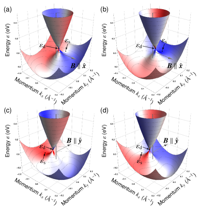
Figure 4: Two-dimensional electron gas with Rashba SOC and in-plane magnetic field along $x$ [(a) and (b)] or $y$ [(c), (d)]. $\varepsilon_{\mathrm{d}}$ and $\varepsilon_{\mathrm{s}}$ are the energy of the degeneracy point and of the saddle point. The color scales represent spin current vorticities $\omega^{x}_{\boldsymbol{k},z}$ [(a), (c)] and $\omega^{y}_{\boldsymbol{k},z}$ [(b), (d); blue/white/red color indicates negative/zero/positive values]. For details, see text.

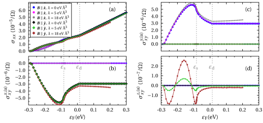
Figure 5: Charge conductivity [(a)] and MSHE [(b)-(d)] in a Rashba system with in-plane magnetic field $\boldsymbol{B}$ and hexagonal warping. Model parameters as for Fig. 4, except for the warping strength $\lambda=$18\text{\,}\mathrm{eV}\text{\,}{\mathrm{\SIUnitSymbolAngstrom}}^{3}$$. For $\lambda=$18\text{\,}\mathrm{eV}\text{\,}{\mathrm{\SIUnitSymbolAngstrom}}^{3}$$, the model is applicable only for $\varepsilon<$0.2\text{\,}\mathrm{eV}$$. For comparison, systems without ($\lambda=0$) and with reduced warping ($\lambda=$5\text{\,}\mathrm{eV}\text{\,}{\mathrm{\SIUnitSymbolAngstrom}}^{3}$$) are considered. Circles (squares) for $\boldsymbol{B}\parallel\hat{\boldsymbol{x}}$ ($\boldsymbol{B}\parallel\hat{\boldsymbol{y}}$); $\underline{\sigma}^{\gamma,\mathrm{(a)}}$ multiplied by $\frac{2e}{\hbar}$ to better compare with the charge conductivity.

IV.2.1 Magnetized Rashba model and its band structure

Recent progress on magnetism in two-dimensional electron gases motivates to demonstrate the existence of SCVs in an in-plane magnetized Rashba model with Hamiltonian

$$\underline{H} =\underbrace{\frac{\hbar^{2}k^{2}}{2m}+\alpha_{\mathrm{R}}\left(k_{x}\underline{\tau}^{y}-k_{y}\underline{\tau}^{x}\right)}_{\underline{H}_{\mathrm{R}}}+\underbrace{\mu_{\mathrm{B}}\boldsymbol{B}\cdot\boldsymbol{\tau}}_{\underline{H}_{\mathrm{Zee}}},$$ (24)

($\underline{\tau}^{i}$ Pauli matrices, $m$ effective mass, and $\alpha_{\mathrm{R}}$ Rashba parameter); hexagonal warping is accounted for later. The continuous rotational symmetry of $\underline{H}_{\mathrm{R}}$ is broken by an in-plane exchange field $\boldsymbol{B}=(B_{x},B_{y},0)^{\mathrm{T}}$ ($\mu_{\mathrm{B}}$ Bohr’s magneton). The set of parameters ($m=0.32\,m_{\mathrm{e}}$, $\alpha_{\mathrm{R}}=2.95\,$\mathrm{eV}\text{\,}\mathrm{\SIUnitSymbolAngstrom}$$, with $m_{\mathrm{e}}$ electron mass) corresponds to those of the ordered $(\sqrt{3}\times\sqrt{3})R30^{\circ}$ Bi/Ag$(111)$ surface alloy Ast et al. (2007); Meier et al. (2008); Bentmann et al. (2009); Frantzeskakis and Grioni (2011); we set $\mu_{\mathrm{B}}B=0.1\,\mathrm{eV}$.

For $\boldsymbol{B}$ in $x$ direction, the two bands are degenerate at a point on the $k_{y}$ axis [panels (a) and (b) of Fig. 4; at energy $\varepsilon_{\mathrm{d}}$]; likewise for $\boldsymbol{B}$ along $y$, the bands are degenerate at a point on the $k_{x}$ axis [(c) and (d)]. On top of that, the lower band has a saddle point at energy $\varepsilon_{\mathrm{s}}$. Overall, the band structure merely exhibits a $k_{x}\to-k_{x}$ [(a), (b)] or a $k_{y}\to-k_{y}$ symmetry [(c), (d)], rendering iso-energy lines anisotropic.

IV.2.2 Symmetries, spin current vorticities, and spin conductivity

With $\boldsymbol{B}$ in $x$ direction ($y$ direction), the model shows nonzero $\varOmega_{x}$ ($\varOmega_{y}$) and, thus, nonzero $\sigma^{y,\mathrm{(a)}}_{xy}$ ($\sigma^{x,\mathrm{(a)}}_{xy}$). Recall that transport takes place in a plane containing the magnetization and that the transported spin component is orthogonal to the magnetization. Since we focus on transport in the $xy$ plane, we consider neither $\sigma^{z,\mathrm{(a)}}_{xz}$ nor $\sigma^{z,\mathrm{(a)}}_{yz}$ although allowed by $\varOmega_{x}$ or $\varOmega_{y}$.

The momentum-resolved SCVs, shown by color in Fig. 4, exhibit a band antisymmetry, $\omega^{x}_{1,\boldsymbol{k},z}=-\omega^{x}_{2,\boldsymbol{k},z}$ and $\omega^{y}_{1,\boldsymbol{k},z}=-\omega^{y}_{2,\boldsymbol{k},z}$ ($1$ and $2$ band indices), which is a feature of a two-band model. Moreover, the SCVs exhibit the following reflection (anti-)symmetries:

$$\boldsymbol{B} \parallel\hat{\boldsymbol{x}}:\quad\omega^{x}_{n,k_{x},k_{y},z}=-\omega^{x}_{n,-k_{x},k_{y},z},\quad\omega^{y}_{n,k_{x},k_{y},z}=\omega^{y}_{n,-k_{x},k_{y},z},$$ (25a)

$$\boldsymbol{B} \parallel\hat{\boldsymbol{y}}:\quad\omega^{x}_{n,k_{x},k_{y},z}=\omega^{x}_{n,k_{x},-k_{y},z},\quad\omega^{y}_{n,k_{x},k_{y},z}=-\omega^{y}_{n,k_{x},-k_{y},z}.$$ (25b)

Even without explicit calculations one verifies that any Fermi sea integral over $\omega^{x}_{\boldsymbol{k},z}$ for $\boldsymbol{B}\parallel\hat{\boldsymbol{x}}$ [panel (a)] or $\omega^{y}_{\boldsymbol{k},z}$ for $\boldsymbol{B}\parallel\hat{\boldsymbol{y}}$ [panel (d)] equals zero due to these antisymmetries. Equation (12) gives $\sigma^{x,\mathrm{(a)}}_{xy}=0$ for $\boldsymbol{B}\parallel\hat{\boldsymbol{x}}$ and $\sigma^{y,\mathrm{(a)}}_{xy}=0$ for $\boldsymbol{B}\parallel\hat{\boldsymbol{y}}$. In contrast, the integrals over $\omega^{y}_{\boldsymbol{k},z}$ for $\boldsymbol{B}\parallel\hat{\boldsymbol{x}}$ (b) or $\omega^{x}_{\boldsymbol{k},z}$ for $\boldsymbol{B}\parallel\hat{\boldsymbol{x}}$ (c) are nonzero, as becomes especially plausible for low energies, at which only red (b) or blue (c) shows up.

For a quantitative analysis, we address the energy dependence of the magnetic spin Hall conductivity. First, we recall that of the charge conductivity $\sigma_{xx}$, as shown in Fig. 5(a). For low Fermi energies $\varepsilon_{\mathrm{F}}$, the direction of the magnetic field strongly affects the shape of the iso-energy lines, leading to different $\sigma_{xx}$ for $\boldsymbol{B}\parallel\hat{\boldsymbol{x}}$ and $\boldsymbol{B}\parallel\hat{\boldsymbol{y}}$, respectively [compare blue and black symbols in Fig. 5(a)]. At higher energies SOC dominates over exchange and, thus, the shape of the iso-energy lines depends marginally on the direction of $\boldsymbol{B}$: there is barely a difference in $\sigma_{xx}$ for $\boldsymbol{B}\parallel\hat{\boldsymbol{x}}$ and $\boldsymbol{B}\parallel\hat{\boldsymbol{y}}$.

For understanding better the energy dependence of the MSHE depicted in Figs. 5(b)–(d), we inspect the SCVs $\omega_{\boldsymbol{k},z}^{x}$, $\omega_{\boldsymbol{k},z}^{y}$, and $\omega_{\boldsymbol{k},z}^{z}$ for $\boldsymbol{B}\parallel\hat{\boldsymbol{x}}$ and $\boldsymbol{B}\parallel\hat{\boldsymbol{y}}$, respectively (Figs. 6 and 7). As expected, $\sigma_{xy}^{x,\mathrm{(a)}}$ ($\sigma_{xy}^{y,\mathrm{(a)}}$) vanishes for $B_{y}=0$ ($B_{x}=0$), which is illustrated in Fig. 6(a) [Fig. 7(b)]: the contributions from Fermi sea regions with positive and negative SCV cancel. In contrast, a finite conductivity $\sigma_{xy}^{y,\mathrm{(a)}}$ ($\sigma_{xy}^{x,\mathrm{(a)}}$) occurs due to incomplete cancellation [Figs. 6(b) and 7(a)].

As sketched in Fig. 4, the bands are degenerate at $\varepsilon_{\mathrm{d}}\approx$8\text{\,}\mathrm{meV}$$. For Fermi levels below the degeneracy, only the lower band is occupied. Increasing the Fermi level from the band edge, the absolute value of $\sigma_{xy}^{y,\mathrm{(a)}}$ ($\sigma_{xy}^{x,\mathrm{(a)}}$) increases [cf. Figs. 5(c) and (b)] due to the growing number of states contributing to the MSHE [cf. black, blue, and green Fermi lines in Figs. 6 or 7].

Around the saddle point at $\varepsilon_{\mathrm{s}}\approx-$83\text{\,}\mathrm{meV}$$ the SCV changes sign and the states contribute oppositely to the magnetic spin Hall conductivity, leading to an extremum of $\sigma_{xy}^{y,\mathrm{(a)}}$ ($\sigma_{xy}^{x,\mathrm{(a)}}$) close to $\varepsilon_{\mathrm{s}}$.

Above $\varepsilon_{\mathrm{d}}$, both bands are occupied (in Figs. 6 and 7, the inner iso-energy line corresponds to the upper band, the outer to the lower band). Only the SCV of the lower band is shown, but the upper band’s SCV differs from the lower band’s only by sign. Thus, regions in $\boldsymbol{k}$ space in which both bands are occupied do not contribute to $\sigma_{xy}^{\gamma,\mathrm{(a)}}$.

With increasing $\varepsilon_{\mathrm{F}}$ the additional contribution of the lower band’s states to the MSHE is compensated by the states in the upper band, thus, $\sigma_{xy}^{y,\mathrm{(a)}}$ and $\sigma_{xy}^{x,\mathrm{(a)}}$ are almost independent of $\varepsilon_{\mathrm{F}}$.

The magnetic spin Hall angle, defined as $\alpha^{\gamma}_{\mathrm{SH}}=\frac{2e}{\hbar}\times 2\sigma^{\gamma,\mathrm{(a)}}_{xy}/(\sigma_{xx}+\sigma_{yy})$ is sizable (up to $70\%$) near the band edge and decreases for larger $\varepsilon_{\mathrm{F}}$. Above $\varepsilon_{\mathrm{d}}$, it is in the order of $10\%$, which may be considered substantial. Its energy dependence is dominated by the almost linear energy dependence of the charge conductivity.

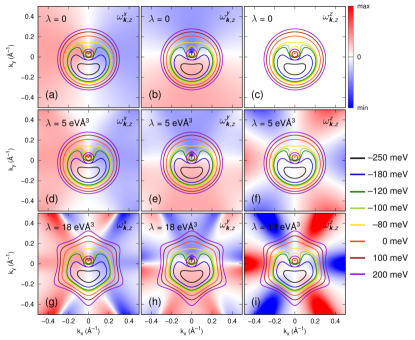
Figure 6: Spin current vorticity (red/blue color scale) and iso-energy lines (colored lines) of the lower band of Rashba systems with and without hexagonal warping in the presence of an in-plane magnetic field $\boldsymbol{B}\parallel\hat{\boldsymbol{x}}$. Model parameters as in Fig. 5.

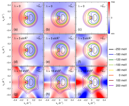
Figure 7: As Fig. 6 but for $\boldsymbol{B}\parallel\hat{\boldsymbol{y}}$.

IV.2.3 Effect of hexagonal warping

To come closer to realistic materials, a hexagonal warping term

$$\underline{H}_{\mathrm{w}}=\frac{\mathrm{i}\lambda}{2}\left(k_{+}^{3}-k_{-}^{3}\right)\underline{\tau}^{z},\quad k_{\pm}=k_{x}\pm\mathrm{i}k_{y},$$ (26)

is added to the Hamiltonian  (24). For $(\sqrt{3}\times\sqrt{3})R30^{\circ}$ Bi/Ag$(111)$, the strength of the warping is $\lambda=$18\text{\,}\mathrm{eV}\text{\,}{\mathrm{\SIUnitSymbolAngstrom}}^{3}$$ Frantzeskakis and Grioni (2011). Similar to the exchange field, $\underline{H}_{\mathrm{w}}$ breaks the continuous rotation symmetry of $\underline{H}_{\mathrm{R}}$, leaving the $xz$ plane as a mirror plane.

For $\boldsymbol{B}\parallel\hat{\boldsymbol{y}}$ this mirror plane is retained (MLG $2/m$; Table 1). Since $\underline{H}_{\mathrm{w}}$ introduces a spin-$z$ component [notice $\underline{\tau}^{z}$ in Eq. (26)], we expect nonzero $\sigma_{xy}^{z,\mathrm{(a)}}$ [associated with $W_{z}^{z}$, as explained in (ii); cf.  Fig. 5(b) and (d)]. For weak warping ($\lambda=$5\text{\,}\mathrm{eV}\text{\,}{\mathrm{\SIUnitSymbolAngstrom}}^{3}$$), the band structure as well as the SCV $\omega_{\boldsymbol{k},z}^{x}$ appear mildly affected by the additional SOC [Fig. 7(d)]. Thus, $\sigma_{xy}^{x,\mathrm{(a)}}$ is weakly influenced by warping. However, a finite spin current vorticity $\omega_{\boldsymbol{k},z}^{z}$ gives rise to a nonzero $\sigma_{xy}^{z,\mathrm{(a)}}$. The sign changes of $\sigma_{xy}^{z,\mathrm{(a)}}$ for $\varepsilon_{\mathrm{F}}<\varepsilon_{\mathrm{s}}$ are due the anisotropy of the Fermi lines and the alternating sign of $\omega_{\boldsymbol{k},z}^{z}$ in reciprocal space [Fig. 7(f) and (i)].

For stronger warping ($\lambda=$18\text{\,}\mathrm{eV}\text{\,}{\mathrm{\SIUnitSymbolAngstrom}}^{3}$$), the energy dispersion and $\omega_{\boldsymbol{k},z}^{x}$ are remarkably modified, which leads to a slightly enhanced MSH conductivity $\sigma_{xy}^{x,\mathrm{(a)}}$ at any $\varepsilon_{\text{F}}$. Furthermore, the absolute value of $\sigma_{xy}^{z,\mathrm{(a)}}$ is increased.

$\boldsymbol{B}\parallel\hat{\boldsymbol{x}}$ makes the $xz$ plane a time-reversal mirror plane (MLG $2^{\prime}/m^{\prime}$; Table 1). Instead of $\sigma_{xy}^{x,\mathrm{(a)}}$ and $\sigma_{xy}^{z,\mathrm{(a)}}$, only $\sigma_{xy}^{y,\mathrm{(a)}}$ is now nonzero [Fig. 5(b)], and its energy dependence is equivalent to that of $\sigma_{xy}^{x,\mathrm{(a)}}$ for $\boldsymbol{B}\parallel\hat{\boldsymbol{y}}$. Note in particular that Figs. 6 (f) and (i) demonstrate that the Fermi sea integral over $\omega_{\boldsymbol{k},z}^{z}$ vanishes for symmetry reasons.

IV.2.4 Concluding remarks and applicability to real materials

To conclude, in-plane magnetized Rashba 2DEGs exhibit a MSHE with in-plane polarized spin current ($\sigma^{x,(a)}_{xy}$ and $\sigma^{y,(a)}_{xy}$) if warping is negligibly small. By rotating the in-plane $\boldsymbol{B}$ field, the transported spin components can be manipulated. On top of that, the interplay of warping and the direction of $\boldsymbol{B}$ allows for nonzero $\sigma^{z,(a)}_{xy}$, thereby causing out-of-plane polarized spin accumulations at the edges of the sample (similar to the conventional SHE). Upon continuous rotation of $\boldsymbol{B}$, the magnetic spin Hall conductivity $\sigma^{z,(a)}_{xy}$ alternates from positive ($\boldsymbol{B}\parallel\hat{\boldsymbol{y}}$) via zero ($\boldsymbol{B}\parallel\pm\hat{\boldsymbol{x}}$) to negative ($\boldsymbol{B}\parallel-\hat{\boldsymbol{y}}$) values.

A similar effect is expected for the warped topological Dirac surface states in Sn-doped Bi₂Te₃ Fu (2009); the exchange field could be induced by proximity to a ferromagnetic insulator Eremeev et al. (2013), a strategy giving rise to an AHE Mogi et al. (2019). Another example is the noncollinear antiferromagnet Mn₃Sn with spin textures as shown in Figs. 8(a) and (d). While the manipulation of in-plane polarized MSHE spin currents by an in-plane field has been successfully demonstrated in Ref. Kimata et al., 2019, the manipulation of the out-of-plane polarized MSHE awaits its experimental confirmation.

The Rashba model for a 2DEG is easily extended to three dimensions, in order to cover multiferroic Rashba semiconductors with bulk Rashba SOC, an example being like (GeMn)Te Krempaský et al. (2016, 2018); Yoshimi et al. (2018). In equilibrium, the magnetization of (GeMn)Te is parallel to the direction of the ferroelectric polarization Krempaský et al. (2016); it is conceivable that an in-plane field causes considerable in-plane canting and a MSHE.

IV.3 Magnetic spin Nernst effect

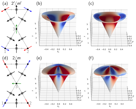
Figure 8: Magnon SCVs for two antiferromagnetic textures on the kagome lattice. Top row: MLG $2^{\prime}/m^{\prime}$. (a) Colored arrows at the vertices and black arrows at the bond centers indicate the spin texture and the DMI vectors for counter-clockwise circulation, respectively. (b) and (c) Dispersion relation of the lowest band in the vicinity of the Brillouin zone center. Color scales indicate the value of the SCVs (b) $\omega^{x}_{\boldsymbol{k},z}$ and (c) $\omega^{y}_{\boldsymbol{k},z}$ (red/white/blue stands for positive/zero/negative SCV). Bottom row: as top row but for the MLG $2/m$. (e) and (f) depict $\omega^{x}_{\boldsymbol{k},z}$ and $\omega^{y}_{\boldsymbol{k},z}$, respectively.

The symmetry considerations of Sec. III.3 apply also to the magnetic spin Nernst effect (MSNE) $\langle\boldsymbol{j}^{\gamma}\rangle=\underline{\alpha}^{\gamma}\,(-\boldsymbol{\nabla}T)$ ($\boldsymbol{\nabla}T$ temperature gradient) which is determined by the antisymmetric part of the magnetothermal conductivity $\underline{\alpha}^{\gamma}$. Within linear-response theory

$$\alpha^{\gamma}_{\mu\nu}(\varpi)= \frac{1}{TV}\int_{0}^{\infty}\mathrm{d}t\,\mathrm{e}^{\mathrm{i}\varpi t}\int_{0}^{\beta}\mathrm{d}\kappa\left\langle Q_{\nu}J^{\gamma}_{\mu}(t+\mathrm{i}\hbar\kappa)\right\rangle+\tilde{\alpha}^{\gamma}_{\mu\nu}(\varpi)$$ (27)

($Q_{\nu}$ total heat current) Han and Lee (2017). $\tilde{\alpha}^{\gamma}_{\mu\nu}(\varpi)$ accounts for circulating equilibrium currents that do not contribute to transport Qin et al. (2011). As far as the intraband contribution is concerned, we write

$$\alpha^{\gamma,\mathrm{odd}}_{\mu\nu,\mathrm{intra}} =\frac{1}{\varGamma TV}\sum_{n,\boldsymbol{k}}J^{\gamma}_{n\boldsymbol{k},\mu}Q_{n\boldsymbol{k},\nu}\left(-\frac{\partial f_{n\boldsymbol{k}}}{\partial\varepsilon}\right)$$ (28)

and derive the MSNE vector

$$\boldsymbol{\alpha}^{\gamma}_{\mathrm{MSNE}} \equiv\frac{1}{2\varGamma TV}\sum_{n,\boldsymbol{k}}\boldsymbol{J}^{\gamma}_{n\boldsymbol{k}}\times\boldsymbol{Q}_{n\boldsymbol{k}}\left(-\frac{\partial f_{n\boldsymbol{k}}}{\partial\varepsilon}\right)$$

$$=-\frac{1}{2\hbar\varGamma T(2\pi)^{3}}\sum_{n}\int_{-\infty}^{\infty}\mathrm{d}\varepsilon\left(\varepsilon-\varepsilon_{\mathrm{F}}\right)\boldsymbol{\omega}^{\gamma}(\varepsilon)\left(-\frac{\partial f_{n\boldsymbol{k}}}{\partial\varepsilon}\right)$$ (29)

using $\boldsymbol{Q}_{n\boldsymbol{k}}=(\varepsilon_{n\boldsymbol{k}}-\varepsilon_{\mathrm{F}})\,\boldsymbol{v}_{n\boldsymbol{k}}$. The SCV $\boldsymbol{\omega}^{\gamma}(\varepsilon)$ at energy $\varepsilon$ is obtained from Eq. (13) by replacing $\varepsilon_{\mathrm{F}}$ by $\varepsilon$. Overall, $\boldsymbol{\alpha}^{\gamma}_{\mathrm{MSNE}}$ and $\boldsymbol{\sigma}^{\gamma}_{\mathrm{MSHE}}$ obey the Mott relation

$$\boldsymbol{\alpha}^{\gamma}_{\mathrm{MSNE}} =-\frac{1}{T}\int_{-\infty}^{\infty}\mathrm{d}\varepsilon\left(-\frac{\partial f_{n\boldsymbol{k}}}{\partial\varepsilon}\right)\frac{\varepsilon-\mu}{e}\boldsymbol{\sigma}^{\gamma}_{\mathrm{MSHE}}(T=0,\varepsilon).$$ (30)

Thus, the symmetry restrictions on $\boldsymbol{\sigma}^{\gamma}_{\mathrm{MSHE}}$ also apply to $\boldsymbol{\alpha}^{\gamma}_{\mathrm{MSNE}}$ and, in particular, the MSNE is also related to the SCV. Consequently, a nonzero MSHE implies a nonzero MSNE.

We now demonstrate the MSNE in magnetic insulators in which $\nabla_{\nu}T$ causes magnonic spin currents. Although the Fermi-Dirac distribution $f_{n\boldsymbol{k}}$ in Eq. (30) has to be replaced by the Bose-Einstein distribution $\rho_{n\boldsymbol{k}}=(\mathrm{e}^{\beta\varepsilon_{n\boldsymbol{k}}}-1)^{-1}$ and the charge current has to be replaced by the particle current, the connection to the SCV remains. Thus, our aim is to show explicitly the existence of a magnonic SCV.

Inspired by the antiferromagnetic magnetic texture of the kagome-lattice compound Mn₃Sn—for which a MSHE was demonstrated in Ref. Kimata et al., 2019—we consider the spin-wave excitations of this texture. Assuming that the kagome plane is not a mirror plane of a surrounding crystal, a minimal spin Hamiltonian reads Elhajal et al. (2002)

$$H=\frac{1}{2\hbar^{2}}\sum_{\langle i,j\rangle}\left(J\boldsymbol{S}_{i}\cdot\boldsymbol{S}_{j}+D_{\parallel}\hat{\boldsymbol{d}}_{ij}\cdot\boldsymbol{S}_{i}\times\boldsymbol{S}_{j}+D_{z}\hat{\boldsymbol{z}}_{ij}\cdot\boldsymbol{S}_{i}\times\boldsymbol{S}_{j}\right).$$ (31)

$J>0$ and $D_{\parallel}$ parametrize the antiferromagnetic exchange and the in-plane Dzyaloshinskii-Moriya interaction [DMI; the unit vectors $\hat{\boldsymbol{d}}_{ij}$ are depicted in Fig. 8(a)], respectively. $D_{z}>0$ is the strength of out-of-plane DMI, with $\hat{\boldsymbol{z}}_{ij}=\pm\hat{\boldsymbol{z}}$; the upper (lower) sign is for (anti-)cyclic indices $ij$.

The out-of-plane DMI $D_{z}>0$ prefers the coplanar magnetic texture of Fig. 8(a) as the classical ground state over the coplanar all-in–all-out configuration (our sign convention is opposite to that in Ref. Elhajal et al., 2002). The corresponding classical ground state energy is independent of $D_{\parallel}$ as long as $|D_{\parallel}/D_{z}|$ is smaller than a critical value (otherwise a canted all-in–all-out texture becomes the energetic minimum Elhajal et al. (2002)). The irrelevance of $D_{\parallel}$ as far as the classical energy is concerned imposes an accidental rotational degeneracy: the spins can be rotated about the $z$ axis without a classical energy penalty, in particular by $\uppi/2$ [Fig. 8(d)]. Since the two textures belong to different magnetic point groups—(a) $2^{\prime}/m^{\prime}$ and (d) $2/m$—there seems to be a ‘classical’ ambiguity concerning spin transport. This ambiguity is lifted upon performing linear spin-wave theory about the two classical magnetic ground states. Following Ref. Mook et al., 2019a, we find that the order-by-quantum-disorder mechanism (harmonic zero-point fluctuations contribute to the ground state energy) prefers texture (a) over (d). Nonetheless, it is instructive to study the SCV for both textures to appreciate the effect of magnetic point group symmetries (details of the linear spin wave theory calculation are given in Appendix A).

We concentrate on low energies because these are most relevant when accounting for thermal occupation (Bose-Einstein distribution). The SCVs $\omega^{x}_{\boldsymbol{k},z}$ and $\omega^{y}_{\boldsymbol{k},z}$ of the lowest magnon band in the vicinity of the Brillouin zone center are given for the MLG $2^{\prime}/m^{\prime}$ in Fig. 8(b) and (e) as well as for the MLG $2/m$ in (c) and (f).

Inspection of panels (b) and (f) tells that for each state $\boldsymbol{k}$ there is a state $\boldsymbol{k}^{\prime}$ with the same energy but with opposite SCV ($\varepsilon_{1,\boldsymbol{k}}=\varepsilon_{1,\boldsymbol{k}^{\prime}}$, $\omega^{\gamma}_{1,\boldsymbol{k},z}=-\omega^{\gamma}_{1,\boldsymbol{k}^{\prime},z}$), a symmetry also found in the Rashba model (Sec. IV.2). Irrespective of the distribution function, the local contributions to the integrated $\omega_{z}^{\gamma}(\varepsilon)$ [Eq. (29)] cancel out: $\alpha_{xy}^{x,(a)}=0$ for the $2^{\prime}/m^{\prime}$ texture and $\alpha_{xy}^{y,(a)}=0$ for the $2/m$ texture. In contrast, the SCVs in Fig. 8(c) and (e) do not exhibit such an antisymmetry and thus have nonzero integral: $\alpha_{xy}^{y,(a)}\neq 0$ for the $2^{\prime}/m^{\prime}$ texture and $\alpha_{xy}^{x,(a)}\neq 0$ for the $2/m$ texture. These findings agree with the $2\times 2$ $xy$ subtensors of $\underline{\sigma}^{x,(a)}$ and $\underline{\sigma}^{y,(a)}$ for both MLGs (Table 1),

$$\underline{\alpha}^{x,(a)}_{2^{\prime}/m^{\prime}}=\begin{pmatrix}0&0\\ 0&0\end{pmatrix}\mbox{\quad and\quad}\underline{\alpha}^{y,(a)}_{2^{\prime}/m^{\prime}}=\begin{pmatrix}0&\alpha^{y}_{xy}\\ -\alpha^{y}_{xy}&0\end{pmatrix},$$ (32a)

$$\underline{\alpha}^{x,(a)}_{2/m}=\begin{pmatrix}0&\alpha^{x}_{xy}\\ -\alpha^{x}_{xy}&0\end{pmatrix}\mbox{\quad and\quad}\underline{\alpha}^{y,(a)}_{2/m}=\begin{pmatrix}0&0\\ 0&0\end{pmatrix}.$$ (32b)

One could expect a finite $\alpha^{z}_{xy}$ for $2/m$, as is the case for the electronic Rashba model studied in Sec. IV.2. For the texture has no out-of-plane component and the magnon spin is defined with respect to the spin directions offered by the ground state texture (Ref. Okuma, 2017 and Appendix A), this component cannot be captured within the present framework. One may regard this a shortcoming of the definition of magnon spin that has to be treated in the future.

V Discussion

As known from the Barnett effect Barnett (1915), a rotating magnetic object is magnetized due to the coupling of angular velocity and spin. Similarly, the vorticity of a fluid couples to spin. Such effects are studied, for example, in nuclear physics Kharzeev et al. (2016) or in the context of spin hydrodynamic generation Takahashi et al. (2016); Matsuo et al. (2017a, b); Doornenbal et al. (2019). Concerning the latter, spin currents brought about by the vorticity of a confined fluid generate nonequilibrium spin voltages. These examples have in common that a vorticity of a fluid in real space is involved. In contrast, the SCV studied here ‘lives’ in momentum space. To put the SCV into a wider context, we show that the concept of vorticity is tightly connected to extrinsic contributions to Hall effects.

Within semiclassical Boltzmann transport theory (e. g., Ref. Popescu et al., 2018) the extrinsic skew scattering contribution to the AHE is given by

$$\boldsymbol{\sigma}^{\mathrm{skew}}_{\mathrm{AHE}} =\frac{1}{2V}\sum_{n\boldsymbol{k}}\boldsymbol{J}_{n\boldsymbol{k}}\times\boldsymbol{\varLambda}_{n\boldsymbol{k}}\left(-\frac{\partial f_{n\boldsymbol{k}}}{\partial\varepsilon}\right),$$ (33)

for which an AHE vector is constructed similar to the MSHE vector in Eq. (10). For a small electric field and a linearized Boltzmann equation, the vectorial mean free path $\boldsymbol{\varLambda}_{n\boldsymbol{k}}$ is obtained from Popescu et al. (2018)

$$\boldsymbol{\varLambda}_{n\boldsymbol{k}}=\frac{1}{\varGamma_{n\boldsymbol{k}}}\left(\boldsymbol{v}_{n\boldsymbol{k}}+\sum_{n^{\prime},\boldsymbol{k}^{\prime}}P^{n\leftarrow n^{\prime}}_{\boldsymbol{k}\leftarrow\boldsymbol{k}^{\prime}}\boldsymbol{\varLambda}_{n^{\prime}\boldsymbol{k}^{\prime}}\right).$$ (34)

$\varGamma_{n\boldsymbol{k}}=\sum_{\boldsymbol{k}^{\prime}}P^{n^{\prime}\leftarrow n}_{\boldsymbol{k}^{\prime}\leftarrow\boldsymbol{k}}$ is the relaxation rate and $P^{n\leftarrow n^{\prime}}_{\boldsymbol{k}\leftarrow\boldsymbol{k}^{\prime}}$ is the scattering rate from a state $(n^{\prime},\boldsymbol{k}^{\prime})$ into a state $(n,\boldsymbol{k})$. The same steps that lead to the SCV yield

$$\boldsymbol{\sigma}^{\mathrm{skew}}_{\mathrm{AHE}} =\frac{-e}{2\hbar(2\pi)^{3}}\sum_{n}\oint_{\varepsilon_{n}=\varepsilon_{\mathrm{F}}}\hat{\boldsymbol{v}}_{n\boldsymbol{k}}\times\boldsymbol{\varLambda}_{n\boldsymbol{k}}\,\mathrm{d}S$$ (35a)

$$=\frac{-e}{2\hbar(2\pi)^{3}}\sum_{n}\iiint_{\varepsilon_{n}\leq\varepsilon_{\mathrm{F}}}\boldsymbol{\nabla}_{\boldsymbol{k}}\times\boldsymbol{\varLambda}_{n\boldsymbol{k}}\,\mathrm{d}^{3}k$$ (35b)

for zero temperature and $\boldsymbol{J}_{n\boldsymbol{k}}=-e\boldsymbol{v}_{n\boldsymbol{k}}$. $\boldsymbol{\nabla}_{\boldsymbol{k}}\times\boldsymbol{\varLambda}_{n\boldsymbol{k}}$ is the vorticity of the mean free path ($\boldsymbol{\varLambda}$ vorticity for short). This means that a scattering process contributes to the AHE if it causes a vorticity in the mean free path; the latter is brought about by the scattering-in terms [sum in Eq. (34)]. To capture the skew scattering contributions to the AHE, the scattering-in terms have to be taken into account, since one finds $\boldsymbol{\boldsymbol{\sigma}}^{\mathrm{skew}}_{\mathrm{AHE}}=\boldsymbol{0}$ if these terms are neglected (e. g. in relaxation time approximation $\boldsymbol{\varLambda}_{n\boldsymbol{k}}=\boldsymbol{v}_{n\boldsymbol{k}}/\varGamma_{n\boldsymbol{k}}$). This reasoning complies with established results for the AHE Nagaosa et al. (2010).

A skewness of the scattering is not necessary for a nonzero SCV, for the latter may be nonzero even in case of a constant relaxation rate $\varGamma_{n\boldsymbol{k}}=\varGamma$ (this is the case considered so far). If the relaxation rate depends on momentum one can still write the MSH conductivity in the form of Eqs. (12) and (13) but with a renormalized SCV

$$\frac{\boldsymbol{\omega}^{\gamma}_{n\boldsymbol{k}}}{\varGamma} \to\tilde{\boldsymbol{\omega}}^{\gamma}_{n\boldsymbol{k}}=\frac{1}{\varGamma_{n\boldsymbol{k}}}\boldsymbol{\omega}^{\gamma}_{n\boldsymbol{k}}-\boldsymbol{J}^{\gamma}_{n\boldsymbol{k}}\times\boldsymbol{\nabla}_{\boldsymbol{k}}\frac{1}{\varGamma_{n\boldsymbol{k}}}.$$ (36)

The original SCV $\boldsymbol{\omega}^{\gamma}_{n\boldsymbol{k}}$ can hence be considered the backbone of the MSHE, on top of which come corrections from skew scattering, side jump or a momentum-dependent relaxation time. Future work may address the MSHE within a quantum kinetic approach, thereby taking into account the electrons’ SU($2$) nature and spin-dependent scattering.

In order to avoid the ill definition of spin current, the authors of Ref. Kimata et al., 2019 considered the MSHE in terms of spin-accumulation rather than of spin-current responses. Such a reasoning fits to present experiments in which spin accumulations rather than spin currents are measured. Nonetheless, the observed spin accumulations may arise from two contributions: a local production (as for the Edelstein effect Aronov and Lyanda-Geller (1989); Edelstein (1990)) and a transport of spins from the bulk toward the edges of the sample.

Compared to the spin current operator $\boldsymbol{J}^{\gamma}$, the velocity does not appear in the time-reversal odd spin operator $s^{\gamma}$. Replacing $\boldsymbol{J}^{\gamma}$ by $s^{\gamma}$ in the Kubo formula implies then that the time-reversal odd and even parts change roles; consequently, spin accumulations brought about by the MSHE appear in the intrinsic part Kimata et al. (2019) and stay finite for $\varGamma\to 0$. The latter finding is to be contrasted with the present theory which predicts a divergence of the bulk spin current in this limit [Eq. (8)]. This variance in one and the same limit suggests that the two underlying mechanisms are fundamentally distinct. To disentangle their relative contribution we propose that future experiments may clarify the role of relaxation processes when taking the clean limit.

VI Concluding remarks

We identified spin current vortices in the Fermi sea as origin of the MSHE. Spin current whirls in reciprocal space provide not only a vivid interpretation of the MSHE but also corroborate that the MSHE has a bulk contribution. Future investigations in which the importance of the bulk and the interfacial contributions is considered could tell how to maximize the MSHE signal. It goes without saying that, due to Onsager’s reciprocity relation Onsager (1931), the SCV also covers an inverse MSHE, that is a transverse charge current caused by a spin bias.

Having identified all magnetic Laue groups that allow for spin current vortices, we demonstrated that any ferromagnet potentially features an MSHE; furthermore, antiferromagnets whose MLG permits a magnetic toroidal quadrupole exhibit an MSHE as well. Two pyrochlore models served as examples (Sec. IV.1) with magnetic textures exhibiting the multipole associated with the MSH conductivities. To issue a caveat, we note that compatibility with a magnetic multipole does not necessitate the presence of the multipole. For example, a completely compensated antiferromagnetic texture may still exhibit symmetries that permit a magnetization, an observation that was appreciated in the context of the AHE for both collinear Šmejkal et al. (2019) as well as noncollinear antiferromagnets Chen et al. (2014); Kübler and Felser (2014); Suzuki et al. (2017). To name two examples: the kagome magnet discussed in Sec. IV.3 admits of a magnetization without exhibiting a net moment, and the magnetic warped Rashba model in Sec. IV.2 admits of magnetic toroidal quadrupoles although the magnetic texture is collinear.

Besides three-dimensional materials, in-plane magnetized Rashba 2DEGs with warping provide a playground for investigating a MSHE. A feature they have in common with Mn₃Sn is the option to manipulate out-of-plane polarized spin currents by rotation of the in-plane magnetic texture. The magnetization provides thus an external means to engineer spin accumulations.

Turning to magnons and replacing the electric field by a temperature gradient, our approach supports that a MSNE is expected but awaits experimental detection. The magnonic MSNE extends the family of magnonic pendants of electronic transport phenomena Mook et al. (2018), its potential for energy harvesting and nonelectronic spin transport remains to be investigated. A candidate material for a proof-of-principle is the ferromagnetic pyrochlore Lu₂V₂O₇. It realizes the magnonic version of the ferromagnetic pyrochlore model of Sec. IV.1 Elhajal et al. (2005) and is known for a thermal Hall effect Onose et al. (2010); Ideue et al. (2012) and for Weyl magnons Mook et al. (2016). For a magnetization and temperature gradient along the $[001]$ direction, we expect magnon-mediated accumulations of magnetic moments, in analogy to the spin accumulations shown in Fig. 1.

Appendix A Linear spin wave theory

We provide some background information on the results presented in Sec. IV.3.

The directions $\hat{\boldsymbol{z}}_{i}$ of the spins in the classical ground state define a local coordinate system $\{\hat{\boldsymbol{x}}_{i},\hat{\boldsymbol{y}}_{i},\hat{\boldsymbol{z}}_{i}\}$. After a (truncated) Holstein-Primakoff transformation Holstein and Primakoff (1940)

$$\frac{\boldsymbol{S}_{i}}{\hbar}\approx\sqrt{\frac{S}{2}}\left[\left(\psi_{i}+\psi_{i}^{\dagger}\right)\hat{\boldsymbol{x}}_{i}-\mathrm{i}\left(\psi_{i}-\psi_{i}^{\dagger}\right)\hat{\boldsymbol{y}}_{i}\right]+\left(S-\psi^{\dagger}_{i}\psi_{i}\right)\hat{\boldsymbol{z}}_{i},$$ (37)

from spin operators to bosonic creation and annihilation operators ($\psi^{\dagger}_{i}$ and $\psi_{i}$), the bilinear Hamiltonian reads

$$H_{2}=\frac{1}{2}\sum_{\boldsymbol{k}}\boldsymbol{\varPsi}^{\dagger}_{\boldsymbol{k}}\underline{H}_{\boldsymbol{k}}\boldsymbol{\varPsi}_{\boldsymbol{k}}$$ (38)

after a Fourier transformation. The vector

$$\boldsymbol{\varPsi}^{\dagger}_{\boldsymbol{k}}=\quantity(\psi^{\dagger}_{1,\boldsymbol{k}},\psi^{\dagger}_{2,\boldsymbol{k}},\psi^{\dagger}_{3,\boldsymbol{k}},\psi_{1,-\boldsymbol{k}},\psi_{2,-\boldsymbol{k}},\psi_{3,-\boldsymbol{k}})$$ (39)

comprises the Fourier transformed bosonic operators $\psi^{(\dagger)}_{n,\boldsymbol{k}}$ ($n=1,2,3$ labels the basis atoms). The linear spin wave kernel

$$\underline{H}_{\boldsymbol{k}} =\frac{S}{2}\begin{pmatrix}\underline{A}_{\boldsymbol{k}}&\underline{B}_{\boldsymbol{k}}\\ \underline{B}^{\dagger}_{\boldsymbol{k}}&\underline{A}^{\ast}_{\boldsymbol{k}}\end{pmatrix}$$ (40)

is built from the submatrices

$$\underline{A}_{\boldsymbol{k}} =\begin{pmatrix}4\left(\sqrt{3}D_{z}+J\right)&q_{1}c_{1}&q_{2}c_{2}\\ q_{1}^{*}c_{1}&4\left(\sqrt{3}D_{z}+J\right)&q_{3}c_{3}\\ q_{2}^{*}c_{2}&q_{3}^{*}c_{3}&4\left(\sqrt{3}D_{z}+J\right)\end{pmatrix}$$ (41)

and

$$\underline{B}_{\boldsymbol{k}} =\begin{pmatrix}0&q_{4}c_{1}&q_{5}c_{2}\\ q_{4}c_{1}&0&q_{6}c_{3}\\ q_{5}c_{2}&q_{6}c_{3}&0\end{pmatrix},$$ (42)

with the $\boldsymbol{k}$-dependent cosines

$$c_{1} =\cos\quantity(ak_{y}),$$ (43a)

$$c_{2} =\cos\left(\frac{a\left(\sqrt{3}k_{x}-k_{y}\right)}{2}\right),$$ (43b)

$$c_{3} =\cos\left(\frac{a\left(\sqrt{3}k_{x}+k_{y}\right)}{2}\right).$$ (43c)

Since the classical ground state is (accidentally) degenerate—the spins can be rigidly rotated within the $xy$ plane without energy cost—the $q_{i}$ ($i=1,\ldots,6$) depend on the chosen ground state.

Here, we consider two textures. The first texture, shown in Fig 8(a), is a representative of the MLG $2^{\prime}/m^{\prime}$; its $q_{i}$ read

$$q_{1} =-\sqrt{3}D_{z}+2\mathrm{i}D_{\parallel}+J,$$ (44a)

$$q_{2} =-\sqrt{3}D_{z}+\mathrm{i}D_{\parallel}+J,$$ (44b)

$$q_{3} =-\sqrt{3}D_{z}-\mathrm{i}D_{\parallel}+J,$$ (44c)

$$q_{4} =-\left(\sqrt{3}D_{z}+3J\right),$$ (44d)

$$q_{5} =-\left(\sqrt{3}D_{z}+3\mathrm{i}D_{\parallel}+3J\right),$$ (44e)

$$q_{6} =-\sqrt{3}D_{z}+3\mathrm{i}D_{\parallel}-3J.$$ (44f)

The second, rotated texture, shown in Fig 8(d), belongs to the MLG $2/m$,

$$q_{1} =-\sqrt{3}D_{z}+J,$$ (45a)

$$q_{2} =-\sqrt{3}D_{z}-\sqrt{3}\mathrm{i}D_{\parallel}+J,$$ (45b)

$$q_{3} =-\sqrt{3}D_{z}-\sqrt{3}\mathrm{i}D_{\parallel}+J,$$ (45c)

$$q_{4} =-\sqrt{3}D_{z}+2\sqrt{3}\mathrm{i}D_{\parallel}-3J,$$ (45d)

$$q_{5} =-\left(\sqrt{3}D_{z}+\sqrt{3}\mathrm{i}D_{\parallel}+3J\right),$$ (45e)

$$q_{6} =q_{5}.$$ (45f)

Next, we diagonalize the bilinear Hamiltonian

$$H_{2}=\frac{1}{2}\sum_{\boldsymbol{k}}\boldsymbol{\varPhi}^{\dagger}_{\boldsymbol{k}}\underline{\mathcal{E}}_{\boldsymbol{k}}\boldsymbol{\varPhi}_{\boldsymbol{k}}.$$ (46)

$\underline{\mathcal{E}}_{\boldsymbol{k}}=\operatorname{\mathop{\mathrm{diag}}}(\varepsilon_{1,\boldsymbol{k}},\varepsilon_{2,\boldsymbol{k}},\varepsilon_{3,\boldsymbol{k}},\varepsilon_{1,-\boldsymbol{k}},\varepsilon_{2,-\boldsymbol{k}},\varepsilon_{3,-\boldsymbol{k}})$ contains the eigenvalues, and $\boldsymbol{\varPhi}_{\boldsymbol{k}}=\quantity(\varPhi_{1,\boldsymbol{k}},\varPhi_{2,\boldsymbol{k}},\varPhi_{3,\boldsymbol{k}},\varPhi^{\dagger}_{1,-\boldsymbol{k}},\varPhi^{\dagger}_{2,-\boldsymbol{k}},\varPhi^{\dagger}_{3,-\boldsymbol{k}})$ is a linear combination of the old bosonic operators,

$$\boldsymbol{\varPhi}^{\dagger}_{\boldsymbol{k}} =\boldsymbol{\varPsi}^{\dagger}_{\boldsymbol{k}}\underline{T}^{\dagger}_{\boldsymbol{k}}.$$ (47)

$\underline{T}_{\boldsymbol{k}}$ diagonalizes $\underline{H}_{\boldsymbol{k}}$ and retains the bosonic commutation rules,

$$\underline{T}^{\dagger}_{\boldsymbol{k}}\,\underline{\varSigma}\,\underline{T}_{\boldsymbol{k}}=\underline{\varSigma},\quad\underline{\varSigma}=\mathrm{diag}(1,1,1,-1,-1,-1).$$ (48)

This procedure follows Ref. Colpa, 1978.

The expectation value of the magnonic spin current of the $n$-th band is defined as Mook et al. (2019b)

$$J^{\gamma}_{n\boldsymbol{k},\mu}=\frac{1}{2}\left.\underline{T}^{\dagger}_{\boldsymbol{k}}\left(\underline{v}_{\boldsymbol{k},\mu}\,\underline{\varSigma}\,\underline{s}^{\gamma}+\underline{s}^{\gamma}\,\underline{\varSigma}\,\underline{v}_{\boldsymbol{k},\mu}\right)\underline{T}_{\boldsymbol{k}}\right|_{n,n},$$ (49)

in which $\underline{v}_{\boldsymbol{k},\mu}=\hbar^{-1}\partial\underline{H}_{\boldsymbol{k}}/\partial k_{\mu}$ is the velocity operator and $\underline{s}^{\gamma}=\mathrm{diag}(z_{1}^{\gamma},z_{2}^{\gamma},z_{3}^{\gamma},z_{1}^{\gamma},z_{2}^{\gamma},z_{3}^{\gamma})$ contains the $\gamma=x,y,z$ coordinate of the local spin directions for the ground state. The magnonic SCV $\boldsymbol{\nabla}_{\boldsymbol{k}}\times\boldsymbol{J}^{\gamma}_{n\boldsymbol{k}}$ is computed numerically; cf. Fig. 8.

References

- Sinova et al. (2015) Jairo Sinova, Sergio O. Valenzuela, J. Wunderlich, C. H. Back, and T. Jungwirth, “Spin Hall effects,” Rev. Mod. Phys. 87, 1213–1260 (2015).
- Kato et al. (2004) Yuichiro K. Kato, Roberto C. Myers, Arthur C. Gossard, and David D. Awschalom, “Observation of the spin Hall effect in semiconductors,” Science 306, 1910–1913 (2004).
- Wunderlich et al. (2005) J. Wunderlich, B. Kaestner, J. Sinova, and T. Jungwirth, “Experimental observation of the spin-Hall effect in a two-dimensional spin-orbit coupled semiconductor system,” Phys. Rev. Lett. 94, 047204 (2005).
- Saitoh et al. (2006) E. Saitoh, M. Ueda, H. Miyajima, and G. Tatara, “Conversion of spin current into charge current at room temperature: Inverse spin-Hall effect,” Applied Physics Letters 88, 182509 (2006).
- Valenzuela and Tinkham (2006) S. O. Valenzuela and M. Tinkham, “Direct electronic measurement of the spin Hall effect,” Nature 442, 176–179 (2006).
- Zhao et al. (2006) Hui Zhao, Eric J. Loren, H. M. van Driel, and Arthur L. Smirl, “Coherence control of Hall charge and spin currents,” Phys. Rev. Lett. 96, 246601 (2006).
- Wolf et al. (2001) S. A. Wolf, D. D. Awschalom, R. A. Buhrman, J. M. Daughton, S. Von Molnar, M. L. Roukes, A. Yu Chtchelkanova, and D. M. Treger, “Spintronics: a spin-based electronics vision for the future,” Science 294, 1488–1495 (2001).
- Žutić et al. (2004) Igor Žutić, Jaroslav Fabian, and S. Das Sarma, “Spintronics: Fundamentals and applications,” Rev. Mod. Phys. 76, 323–410 (2004).
- Jungwirth et al. (2012) Tomas Jungwirth, Jörg Wunderlich, and Kamil Olejník, “Spin Hall effect devices,” Nature materials 11, 382 (2012).
- Chernyshov et al. (2009) Alexandr Chernyshov, Mason Overby, Xinyu Liu, Jacek K. Furdyna, Yuli Lyanda-Geller, and Leonid P. Rokhinson, “Evidence for reversible control of magnetization in a ferromagnetic material by means of spin–orbit magnetic field,” Nature Physics 5, 656 (2009).
- Liu et al. (2011) Luqiao Liu, Takahiro Moriyama, D. C. Ralph, and R. A. Buhrman, “Spin-torque ferromagnetic resonance induced by the spin Hall effect,” Phys. Rev. Lett. 106, 036601 (2011).
- Liu et al. (2012) L. Liu, C.-F. Pai, Y. Li, H. W. Tseng, D. C. Ralph, and R. A. Buhrman, “Spin-torque switching with the giant spin Hall effect of tantalum,” Science 336, 555–558 (2012).
- Slonczewski (1996) J.C. Slonczewski, “Current-driven excitation of magnetic multilayers,” Journal of Magnetism and Magnetic Materials 159, L1–L7 (1996).
- Berger (1996) L. Berger, “Emission of spin waves by a magnetic multilayer traversed by a current,” Phys. Rev. B 54, 9353–9358 (1996).
- Ralph and Stiles (2008) D.C. Ralph and M.D. Stiles, “Spin transfer torques,” Journal of Magnetism and Magnetic Materials 320, 1190–1216 (2008).
- Brataas et al. (2012) Arne Brataas, Andrew D. Kent, and Hideo Ohno, “Current-induced torques in magnetic materials,” Nature Materials 11, 372–381 (2012).
- Khvalkovskiy et al. (2013) A. V. Khvalkovskiy, D. Apalkov, S. Watts, R. Chepulskii, R. S. Beach, A. Ong, X. Tang, A. Driskill-Smith, W. H. Butler, P. B. Visscher, D. Lottis, E. Chen, V. Nikitin, and M. Krounbi, “Basic principles of STT-MRAM cell operation in memory arrays,” Journal of Physics D: Applied Physics 46, 074001 (2013).
- Gambardella and Miron (2011) Pietro Gambardella and Ioan Mihai Miron, “Current-induced spin–orbit torques,” Philosophical Transactions of the Royal Society A: Mathematical, Physical and Engineering Sciences 369, 3175–3197 (2011).
- Jabeur et al. (2014) Kotb Jabeur, Gregory Di Pendina, Fabrice Bernard-Granger, and Guillaume Prenat, “Spin orbit torque non-volatile flip-flop for high speed and low energy applications,” IEEE Electron Device Letters 35, 408–410 (2014).
- Prenat et al. (2016) Guillaume Prenat, Kotb Jabeur, Pierre Vanhauwaert, Gregory Di Pendina, Fabian Oboril, Rajendra Bishnoi, Mojtaba Ebrahimi, Nathalie Lamard, Olivier Boulle, Kevin Garello, Juergen Langer, Berthold Ocker, Marie-Claire Cyrille, Pietro Gambardella, Mehdi Tahoori, and Gilles Gaudin, “Ultra-fast and high-reliability SOT-MRAM: From cache replacement to normally-off computing,” IEEE Transactions on Multi-Scale Computing Systems 2, 49–60 (2016).
- Li et al. (2018) Yucai Li, Kevin William Edmonds, Xionghua Liu, Houzhi Zheng, and Kaiyou Wang, “Manipulation of magnetization by spin-orbit torque,” Advanced Quantum Technologies 2, 1800052 (2018).
- Nagaosa et al. (2010) Naoto Nagaosa, Jairo Sinova, Shigeki Onoda, A. H. MacDonald, and N. P. Ong, “Anomalous Hall effect,” Rev. Mod. Phys. 82, 1539–1592 (2010).
- S. Murakami and Zhang (2003) N. Nagaosa S. Murakami and S.-C. Zhang, “Dissipationless quantum spin current at room temperature,” Science 301, 1348–1351 (2003).
- Sinova et al. (2004) Jairo Sinova, Dimitrie Culcer, Q. Niu, N. A. Sinitsyn, T. Jungwirth, and A. H. MacDonald, “Universal intrinsic spin Hall effect,” Phys. Rev. Lett. 92, 126603 (2004).
- Dyakonov and Perel (1971) M.I. Dyakonov and V.I. Perel, “Current-induced spin orientation of electrons in semiconductors,” Physics Letters A 35, 459–460 (1971).
- Hirsch (1999) J. E. Hirsch, “Spin Hall effect,” Phys. Rev. Lett. 83, 1834–1837 (1999).
- Zhang (2000) Shufeng Zhang, “Spin Hall effect in the presence of spin diffusion,” Phys. Rev. Lett. 85, 393–396 (2000).
- Mott (1929) N. F. Mott, “The scattering of fast electrons by atomic nuclei,” Proceedings of the Royal Society A: Mathematical, Physical and Engineering Sciences 124, 425–442 (1929).
- Guo et al. (2008) G. Y. Guo, S. Murakami, T.-W. Chen, and N. Nagaosa, “Intrinsic spin Hall effect in platinum: First-principles calculations,” Phys. Rev. Lett. 100, 096401 (2008).
- Zhang et al. (2018a) Yang Zhang, Jakub Železnỳ, Yan Sun, Jeroen van den Brink, and Binghai Yan, “Spin Hall effect emerging from a noncollinear magnetic lattice without spin–orbit coupling,” New Journal of Physics 20, 073028 (2018a).
- Miao et al. (2013) B. F. Miao, S. Y. Huang, D. Qu, and C. L. Chien, “Inverse spin Hall effect in a ferromagnetic metal,” Phys. Rev. Lett. 111, 066602 (2013).
- Taniguchi et al. (2015) Tomohiro Taniguchi, J. Grollier, and M. D. Stiles, “Spin-transfer torques generated by the anomalous Hall effect and anisotropic magnetoresistance,” Phys. Rev. Applied 3, 044001 (2015).
- Tian et al. (2016) Dai Tian, Yufan Li, D. Qu, S. Y. Huang, Xiaofeng Jin, and C. L. Chien, “Manipulation of pure spin current in ferromagnetic metals independent of magnetization,” Phys. Rev. B 94, 020403 (2016).
- Wu et al. (2017) H. Wu, X. Wang, L. Huang, J.Y. Qin, C. Fang, X. Zhang, C.H. Wan, and X.F. Han, “Separation of inverse spin Hall effect and anomalous Nernst effect in ferromagnetic metals,” Journal of Magnetism and Magnetic Materials 441, 149–153 (2017).
- Das et al. (2017) K. S. Das, W. Y. Schoemaker, B. J. van Wees, and I. J. Vera-Marun, “Spin injection and detection via the anomalous spin Hall effect of a ferromagnetic metal,” Phys. Rev. B 96, 220408 (2017).
- Humphries et al. (2017) Alisha M. Humphries, Tao Wang, Eric R. J. Edwards, Shane R. Allen, Justin M. Shaw, Hans T. Nembach, John Q. Xiao, T. J. Silva, and Xin Fan, “Observation of spin-orbit effects with spin rotation symmetry,” Nature Communications 8, 911 (2017).
- Amin et al. (2018) V. P. Amin, J. Zemen, and M. D. Stiles, “Interface-generated spin currents,” Phys. Rev. Lett. 121, 136805 (2018).
- Gibbons et al. (2018) Jonathan D. Gibbons, David MacNeill, Robert A. Buhrman, and Daniel C. Ralph, “Reorientable spin direction for spin current produced by the anomalous Hall effect,” Phys. Rev. Applied 9, 064033 (2018).
- Bose et al. (2018) Arnab Bose, D. D. Lam, S. Bhuktare, S. Dutta, H. Singh, Y. Jibiki, M. Goto, S. Miwa, and A. A. Tulapurkar, “Observation of anomalous spin torque generated by a ferromagnet,” Phys. Rev. Applied 9, 064026 (2018).
- Baek et al. (2018) Seung-heon C. Baek, Vivek P. Amin, Young-Wan Oh, Gyungchoon Go, Seung-Jae Lee, Geun-Hee Lee, Kab-Jin Kim, M. D. Stiles, Byong-Guk Park, and Kyung-Jin Lee, “Spin currents and spin-orbit torques in ferromagnetic trilayers,” Nature Materials 17, 509–513 (2018).
- Omori et al. (2019) Yasutomo Omori, Edurne Sagasta, Yasuhiro Niimi, Martin Gradhand, Luis E. Hueso, Fèlix Casanova, and YoshiChika Otani, “Relation between spin Hall effect and anomalous Hall effect in ferromagnetic metals,” Phys. Rev. B 99, 014403 (2019).
- Amin et al. (2019) V. P. Amin, Junwen Li, M. D. Stiles, and P. M. Haney, “Intrinsic spin currents in ferromagnets,” (2019).
- Qu et al. (2019) Guanxiong Qu, Kohji Nakamura, and Masamitsu Hayashi, “Magnetization direction dependent spin Hall effect in 3d ferromagnets,” (2019), arXiv:1901.10740 .
- Wang et al. (2019) Wenrui Wang, Tao Wang, Vivek P. Amin, Yang Wang, Anil Radhakrishnan, Angie Davidson, Shane R. Allen, T. J. Silva, Hendrik Ohldag, Davor Balzar, Barry L. Zink, Paul M. Haney, John Q. Xiao, David G. Cahill, Virginia O. Lorenz, and Xin Fan, “Anomalous spin-orbit torques in magnetic single-layer films,” Nature Nanotechnology 14, 819–824 (2019).
- Železný et al. (2017) Jakub Železný, Yang Zhang, Claudia Felser, and Binghai Yan, “Spin-polarized current in noncollinear antiferromagnets,” Phys. Rev. Lett. 119, 187204 (2017).
- Železný et al. (2018) J. Železný, P. Wadley, K. Olejník, A. Hoffmann, and H. Ohno, “Spin transport and spin torque in antiferromagnetic devices,” Nature Physics 14, 220–228 (2018).
- Chen et al. (2018) Hua Chen, Qian Niu, and Allan H. MacDonald, “Spin Hall effect without spin currents in magnetic insulators,” (2018), arXiv:1803.01294 .
- Kimata et al. (2019) Motoi Kimata, Hua Chen, Kouta Kondou, Satoshi Sugimoto, Prasanta K. Muduli, Muhammad Ikhlas, Yasutomo Omori, Takahiro Tomita, Allan H. MacDonald, Satoru Nakatsuji, and Yoshichika Otani, “Magnetic and magnetic inverse spin Hall effects in a non-collinear antiferromagnet,” Nature (2019), 10.1038/s41586-018-0853-0.
- Wimmer et al. (2015) S. Wimmer, M. Seemann, K. Chadova, D. Ködderitzsch, and H. Ebert, “Spin-orbit-induced longitudinal spin-polarized currents in nonmagnetic solids,” Phys. Rev. B 92, 041101 (2015).
- Seemann et al. (2015) M. Seemann, D. Ködderitzsch, S. Wimmer, and H. Ebert, “Symmetry-imposed shape of linear response tensors,” Phys. Rev. B 92, 155138 (2015).
- MacNeill et al. (2016) D. MacNeill, G. M. Stiehl, M. H. D. Guimaraes, R. A. Buhrman, J. Park, and D. C. Ralph, “Control of spin-orbit torques through crystal symmetry in wte2/ferromagnet bilayers,” Nature Physics 13, 300 EP – (2016), article.
- Zhou et al. (2019) Jiaqi Zhou, Junfeng Qiao, Arnaud Bournel, and Weisheng Zhao, “Intrinsic spin Hall conductivity of the semimetals MoTe2 and WTe2,” Phys. Rev. B 99, 060408 (2019).
- Davidson et al. (2019) Angie Davidson, Vivek P. Amin, Wafa S. Aljuaid, Paul M. Haney, and Xin Fan, “Perspectives of electrically generated spin currents in ferromagnetic materials,” (2019), arXiv:1906.11772 .
- Hönemann et al. (2019) Albert Hönemann, Christian Herschbach, Dmitry V. Fedorov, Martin Gradhand, and Ingrid Mertig, “Spin and charge currents induced by the spin Hall and anomalous Hall effects upon crossing ferromagnetic/nonmagnetic interfaces,” Phys. Rev. B 99, 024420 (2019).
- Lesne et al. (2016) E. Lesne, Yu Fu, S. Oyarzun, J. C. Rojas-Sánchez, D. C. Vaz, H. Naganuma, G. Sicoli, J.-P. Attané, M. Jamet, E. Jacquet, J.-M. George, A. Barthélémy, H. Jaffrès, A. Fert, M. Bibes, and L. Vila, “Highly efficient and tunable spin-to-charge conversion through Rashba coupling at oxide interfaces,” Nature Materials 15, 1261–1266 (2016).
- Brinkman et al. (2007) A. Brinkman, M. Huijben, M. van Zalk, J. Huijben, U. Zeitler, J. C. Maan, W. G. van der Wiel, G. Rijnders, D. H. A. Blank, and H. Hilgenkamp, “Magnetic effects at the interface between non-magnetic oxides,” Nature Materials 6, 493–496 (2007).
- Reyren et al. (2007) N. Reyren, S. Thiel, A. D. Caviglia, L. F. Kourkoutis, G. Hammerl, C. Richter, C. W. Schneider, T. Kopp, A.-S. Ruetschi, D. Jaccard, M. Gabay, D. A. Muller, J.-M. Triscone, and J. Mannhart, “Superconducting interfaces between insulating oxides,” Science 317, 1196–1199 (2007).
- Bert et al. (2011) Julie A. Bert, Beena Kalisky, Christopher Bell, Minu Kim, Yasuyuki Hikita, Harold Y. Hwang, and Kathryn A. Moler, “Direct imaging of the coexistence of ferromagnetism and superconductivity at the LaAlO3/SrTiO3 interface,” Nature Physics 7, 767–771 (2011).
- Dikin et al. (2011) D. A. Dikin, M. Mehta, C. W. Bark, C. M. Folkman, C. B. Eom, and V. Chandrasekhar, “Coexistence of superconductivity and ferromagnetism in two dimensions,” Phys. Rev. Lett. 107, 056802 (2011).
- Li et al. (2011) Lu Li, C. Richter, J. Mannhart, and R. C. Ashoori, “Coexistence of magnetic order and two-dimensional superconductivity at LaAlO3/SrTiO3 interfaces,” Nature Physics 7, 762–766 (2011).
- Joshua et al. (2012) Arjun Joshua, S Pecker, J Ruhman, E Altman, and S Ilani, “A universal critical density underlying the physics of electrons at the LaAlO3/SrTiO3 interface,” Nature communications 3, 1129 (2012).
- Caviglia et al. (2008) A. D. Caviglia, S. Gariglio, N. Reyren, D. Jaccard, T. Schneider, M. Gabay, S. Thiel, G. Hammerl, J. Mannhart, and J.-M. Triscone, “Electric field control of the LaAlO3/SrTiO3 interface ground state,” Nature 456, 624–627 (2008).
- Zhang et al. (2018b) Hongrui Zhang, Xi Yan, Hui Zhang, Fei Wang, Youdi Gu, Xingkun Ning, Tahira Khan, Rui Li, Yuansha Chen, Wei Liu, Shufang Wang, Baogen Shen, and Jirong Sun, “Magnetic two-dimensional electron gases with high Curie temperatures at LaAlO3/SrTiOfe interfaces,” Phys. Rev. B 97, 155150 (2018b).
- Fu (2009) Liang Fu, “Hexagonal warping effects in the surface states of the topological insulator Bi2Te3,” Phys. Rev. Lett. 103, 266801 (2009).
- Eremeev et al. (2013) S. V. Eremeev, V. N. Men’shov, V. V. Tugushev, P. M. Echenique, and E. V. Chulkov, “Magnetic proximity effect at the three-dimensional topological insulator/magnetic insulator interface,” Phys. Rev. B 88, 144430 (2013).
- Kubo et al. (1957) Ryogo Kubo, Mario Yokota, and Sadao Nakajima, “Statistical-mechanical theory of irreversible processes. II. Response to thermal disturbance,” Journal of the Physical Society of Japan 12, 1203–1211 (1957).
- Mahan (2000) Gerald D. Mahan, Many-Particle Physics (Springer Science + Business Media, 2000).
- Landau and Lifshitz (2013) L D Landau and E. M. Lifshitz, Fluid Mechanics: Landau and Lifshitz: Course of Theoretical Physics, Volume 6 (Pergamon, 2013).
- Roux and Fink (1995) Ph. Roux and M. Fink, “Experimental evidence in acoustics of the violation of time-reversal invariance induced by vorticity,” EPL (Europhysics Letters) 32, 25 (1995).
- Kleiner (1966) W. H. Kleiner, “Space-time symmetry of transport coefficients,” Phys. Rev. 142, 318–326 (1966).
- Kleiner (1967) W. H. Kleiner, “Space-time symmetry restrictions on transport coefficients. ii. Two theories compared,” Phys. Rev. 153, 726–727 (1967).
- Kleiner (1969) W. H. Kleiner, “Space-time symmetry restrictions on transport coefficients. iii. Thermogalvanomagnetic coefficients,” Phys. Rev. 182, 705–709 (1969).
- Nanz (2016) Stefan Nanz, “Why another multipole family?” in Toroidal Multipole Moments in Classical Electrodynamics (Springer Fachmedien Wiesbaden, 2016) pp. 5–11.
- Jahn (1949) H. A. Jahn, “Note on the Bhagavantam–Suranarayana method of enumerating the physical constants of crystals,” Acta Crystallographica 2, 30–33 (1949).
- Hayami et al. (2018) Satoru Hayami, Megumi Yatsushiro, Yuki Yanagi, and Hiroaki Kusunose, “Classification of atomic-scale multipoles under crystallographic point groups and application to linear response tensors,” Phys. Rev. B 98, 165110 (2018).
- Gallego et al. (2019) Samuel V. Gallego, Jesus Etxebarria, Luis Elcoro, Emre S. Tasci, and J. Manuel Perez-Mato, “Automatic calculation of symmetry-adapted tensors in magnetic and non-magnetic materials: a new tool of the Bilbao Crystallographic Server,” Acta Crystallographica Section A 75, 438–447 (2019).
- Aroyo et al. (2006a) Mois Ilia Aroyo, Juan Manuel Perez-Mato, Cesar Capillas, Eli Kroumova, Svetoslav Ivantchev, Gotzon Madariaga, Asen Kirov, and Hans Wondratschek, “Bilbao crystallographic server: I. Databases and crystallographic computing programs,” Zeitschrift für Kristallographie - Crystalline Materials 221 (2006a), 10.1524/zkri.2006.221.1.15.
- Aroyo et al. (2006b) Mois I. Aroyo, Asen Kirov, Cesar Capillas, J. M. Perez-Mato, and Hans Wondratschek, “Bilbao crystallographic server. II. Representations of crystallographic point groups and space groups,” Acta Crystallographica Section A Foundations of Crystallography 62, 115–128 (2006b).
- Aroyo et al. (2011) Mois I. Aroyo, J.M. Perez-Mato, D. Orobengoa, E. Tasci, G. De La Flor, and A. Kirov, “Crystallography online: Bilbao crystallographic server,” Bulgarian Chemical Communications 43, 183–197 (2011).
- Note (1) If the spin orientation breaks all crystal symmetries, Mn3Sn belongs to the MLG , which is, however, unlikely in the absence of a magnetic field, because of anisotropies along high symmetry directions of the lattice.
- Bzdušek et al. (2015) Tomáš Bzdušek, Andreas Rüegg, and Manfred Sigrist, “Weyl semimetal from spontaneous inversion symmetry breaking in pyrochlore oxides,” Phys. Rev. B 91, 165105 (2015).
- Suzuki et al. (2019) M.-T. Suzuki, T. Nomoto, R. Arita, Y. Yanagi, S. Hayami, and H. Kusunose, “Multipole expansion for magnetic structures: A generation scheme for a symmetry-adapted orthonormal basis set in the crystallographic point group,” Phys. Rev. B 99, 174407 (2019).
- Ast et al. (2007) Christian R. Ast, Jürgen Henk, Arthur Ernst, Luca Moreschini, Mihaela C. Falub, Daniela Pacilé, Patrick Bruno, Klaus Kern, and Marco Grioni, “Giant spin splitting through surface alloying,” Phys. Rev. Lett. 98, 186807 (2007).
- Meier et al. (2008) Fabian Meier, Hugo Dil, Jorge Lobo-Checa, Luc Patthey, and Jürg Osterwalder, “Quantitative vectorial spin analysis in angle-resolved photoemission: Bi/Ag and Pb/Ag,” Phys. Rev. B 77, 165431 (2008).
- Bentmann et al. (2009) H. Bentmann, F. Forster, G. Bihlmayer, E. V. Chulkov, L. Moreschini, M. Grioni, and F. Reinert, “Origin and manipulation of the Rashba splitting in surface alloys,” EPL (Europhysics Letters) 87, 37003 (2009).
- Frantzeskakis and Grioni (2011) Emmanouil Frantzeskakis and Marco Grioni, “Anisotropy effects on Rashba and topological insulator spin-polarized surface states: A unified phenomenological description,” Phys. Rev. B 84, 155453 (2011).
- Mogi et al. (2019) Masataka Mogi, Taro Nakajima, Victor Ukleev, Atsushi Tsukazaki, Ryutaro Yoshimi, Minoru Kawamura, Kei S. Takahashi, Takayasu Hanashima, Kazuhisa Kakurai, Taka-hisa Arima, Masashi Kawasaki, and Yoshinori Tokura, “Large anomalous Hall effect in topological insulators with proximitized ferromagnetic insulators,” Phys. Rev. Lett. 123, 016804 (2019).
- Krempaský et al. (2016) J. Krempaský, S. Muff, F. Bisti, M. Fanciulli, H. Volfová, A. P. Weber, N. Pilet, P. Warnicke, H. Ebert, J. Braun, F. Bertran, V. V. Volobuev, J. Minár, G. Springholz, J. H. Dil, and V. N. Strocov, “Entanglement and manipulation of the magnetic and spin–orbit order in multiferroic Rashba semiconductors,” Nature Communications 7 (2016), 10.1038/ncomms13071.
- Krempaský et al. (2018) J. Krempaský, G. Springholz, J. Minár, and J. H. Dil, “-GeTe and (GeMn)Te semiconductors: A new paradigm for spintronics,” AIP Conference Proceedings 1996, 020026 (2018), https://aip.scitation.org/doi/pdf/10.1063/1.5048878 .
- Yoshimi et al. (2018) R. Yoshimi, K. Yasuda, A. Tsukazaki, K. S. Takahashi, M. Kawasaki, and Y. Tokura, “Current-driven magnetization switching in ferromagnetic bulk Rashba semiconductor (Ge, Mn)Te,” Science Advances 4, eaat9989 (2018).
- Han and Lee (2017) Jung Hoon Han and Hyunyong Lee, “Spin chirality and Hall-like transport phenomena of spin excitations,” Journal of the Physical Society of Japan 86, 011007 (2017).
- Qin et al. (2011) Tao Qin, Qian Niu, and Junren Shi, “Energy magnetization and the thermal Hall effect,” Phys. Rev. Lett. 107, 236601 (2011).
- Elhajal et al. (2002) M. Elhajal, B. Canals, and C. Lacroix, “Symmetry breaking due to Dzyaloshinsky-Moriya interactions in the kagomé lattice,” Phys. Rev. B 66, 014422 (2002).
- Mook et al. (2019a) Alexander Mook, Jürgen Henk, and Ingrid Mertig, “Thermal Hall effect in noncollinear coplanar insulating antiferromagnets,” Phys. Rev. B 99, 014427 (2019a).
- Okuma (2017) Nobuyuki Okuma, “Magnon spin-momentum locking: Various spin vortices and Dirac magnons in noncollinear antiferromagnets,” Phys. Rev. Lett. 119, 107205 (2017).
- Barnett (1915) S. J. Barnett, “Magnetization by rotation,” Phys. Rev. 6, 239–270 (1915).
- Kharzeev et al. (2016) D.E. Kharzeev, J. Liao, S.A. Voloshin, and G. Wang, “Chiral magnetic and vortical effects in high-energy nuclear collisions—a status report,” Progress in Particle and Nuclear Physics 88, 1 – 28 (2016).
- Takahashi et al. (2016) R. Takahashi, M. Matsuo, M. Ono, K. Harii, H. Chudo, S. Okayasu, J. Ieda, S. Takahashi, S. Maekawa, and E. Saitoh, “Spin hydrodynamic generation,” Nature Physics 12, 52 (2016).
- Matsuo et al. (2017a) Mamoru Matsuo, Eiji Saitoh, and Sadamichi Maekawa, “Spin-Mechatronics,” Journal of the Physical Society of Japan 86, 011011 (2017a).
- Matsuo et al. (2017b) M. Matsuo, Y. Ohnuma, and S. Maekawa, “Theory of spin hydrodynamic generation,” Phys. Rev. B 96, 020401 (2017b).
- Doornenbal et al. (2019) Ruben J. Doornenbal, Marco Polini, and Rembert A. Duine, “Spin–vorticity coupling in viscous electron fluids,” Journal of Physics: Materials 2, 015006 (2019).
- Popescu et al. (2018) Voicu Popescu, Peter Kratzer, Peter Entel, Christian Heiliger, Michael Czerner, Katarina Tauber, Franziska Töpler, Christian Herschbach, Dmitry V Fedorov, Martin Gradhand, Ingrid Mertig, Roman Kováčik, Phivos Mavropoulos, Daniel Wortmann, Stefan Blügel, Frank Freimuth, Yuriy Mokrousov, Sebastian Wimmer, Diemo Ködderitzsch, Marten Seemann, Kristina Chadova, and Hubert Ebert, “Spin caloric transport from density-functional theory,” Journal of Physics D: Applied Physics 52, 073001 (2018).
- Aronov and Lyanda-Geller (1989) A. G. Aronov and Yu B. Lyanda-Geller, “Nuclear electric resonance and orientation of carrier spins by an electric field,” Soviet Journal of Experimental and Theoretical Physics Letters 50, 431 (1989).
- Edelstein (1990) V.M. Edelstein, “Spin polarization of conduction electrons induced by electric current in two-dimensional asymmetric electron systems,” Solid State Communications 73, 233–235 (1990).
- Onsager (1931) Lars Onsager, “Reciprocal relations in irreversible processes. I.” Phys. Rev. 37, 405–426 (1931).
- Šmejkal et al. (2019) Libor Šmejkal, Rafael González-Hernández, Tomáš Jungwirth, and Jairo Sinova, “Crystal Hall effect in collinear antiferromagnets,” (2019), arXiv:1901.00445 .
- Chen et al. (2014) Hua Chen, Qian Niu, and A. H. MacDonald, “Anomalous Hall effect arising from noncollinear antiferromagnetism,” Phys. Rev. Lett. 112, 017205 (2014).
- Kübler and Felser (2014) Jürgen Kübler and Claudia Felser, “Non-collinear antiferromagnets and the anomalous Hall effect,” EPL (Europhysics Letters) 108, 67001 (2014).
- Suzuki et al. (2017) M.-T. Suzuki, T. Koretsune, M. Ochi, and R. Arita, “Cluster multipole theory for anomalous Hall effect in antiferromagnets,” Phys. Rev. B 95, 094406 (2017).
- Mook et al. (2018) Alexander Mook, Börge Göbel, Jürgen Henk, and Ingrid Mertig, “Taking an electron-magnon duality shortcut from electron to magnon transport,” Phys. Rev. B 97, 140401 (2018).
- Elhajal et al. (2005) Maged Elhajal, Benjamin Canals, Raimon Sunyer, and Claudine Lacroix, “Ordering in the pyrochlore antiferromagnet due to Dzyaloshinsky-Moriya interactions,” Phys. Rev. B 71, 094420 (2005).
- Onose et al. (2010) Y. Onose, T. Ideue, H. Katsura, Y. Shiomi, N. Nagaosa, and Y. Tokura, “Observation of the magnon hall effect,” Science 329, 297–299 (2010).
- Ideue et al. (2012) T. Ideue, Y. Onose, H. Katsura, Y. Shiomi, S. Ishiwata, N. Nagaosa, and Y. Tokura, “Effect of lattice geometry on magnon Hall effect in ferromagnetic insulators,” Phys. Rev. B 85, 134411 (2012).
- Mook et al. (2016) Alexander Mook, Jürgen Henk, and Ingrid Mertig, “Tunable magnon Weyl points in ferromagnetic pyrochlores,” Phys. Rev. Lett. 117, 157204 (2016).
- Holstein and Primakoff (1940) T. Holstein and H. Primakoff, “Field dependence of the intrinsic domain magnetization of a ferromagnet,” Phys. Rev. 58, 1098–1113 (1940).
- Colpa (1978) J.H.P. Colpa, “Diagonalization of the quadratic boson hamiltonian,” Physica A: Statistical Mechanics and its Applications 93, 327–353 (1978).
- Mook et al. (2019b) Alexander Mook, Robin R. Neumann, Jürgen Henk, and Ingrid Mertig, “Spin Seebeck and spin Nernst effects of magnons in noncollinear antiferromagnetic insulators,” Phys. Rev. B 100, 100401 (2019b).