Roles of repertoire diversity in robustness of humoral immune response

Abstract

The adaptive immune system relies on diversity of its repertoire of receptors to protect the organism from a great variety of pathogens. Since the initial repertoire is the result of random gene rearrangement, binding of receptors is not limited to pathogen-associated antigens but also includes self antigens. There is a fine balance between having a diverse repertoire, protecting from many different pathogens, and yet reducing its self-reactivity as far as possible to avoid damage to self. In the ageing immune system this balance is altered, manifesting in reduced specificity of response to pathogens or vaccination on a background of higher self-reactivity. To answer the question whether age-related changes of repertoire in the diversity and self/non-self affinity balance of antibodies could explain the reduced efficacy of the humoral response in older people, we construct a minimal mathematical model of the humoral immune response. The principle of least damage allows us, for a given repertoire of antibodies, to resolve a tension between the necessity to neutralise target antigens as quickly as possible and the requirement to limit the damage to self antigens leading to an optimal dynamics of immune response. The model predicts slowing down of immune response for repertoires with reduced diversity and increased self-reactivity.

This manuscript was compiled on

The adaptive immune system relies on an extremely diverse repertoire of receptors that can recognise target molecules to protect us from pathogens. Each cell has a unique specificity, encoded by the T cell receptor on T cells, or the B cell receptor on B cells. In the case of B cells, the B cell receptor is also known as surface immunoglobulin, and this immunoglobulin (Ig) can be secreted as antibody once the cell has developed into a plasma cell. Antibodies (Ab) are an important first line of defence, they can block the action of harmful target molecules and help to recruit additional elements of the immune system by acting as bridges between target molecules and effector cells. The targets of Ab are known as antigens (Ag).

B cells are formed in the bone marrow, where they acquire a unique Ig via gene rearrangement, a process that can produce over $10^{8}$ different genes by reassortment of less than 200 germline gene segments (1, 2). The highest diversity is seen in the areas of the Ig gene where different gene segments are joined together, and these areas of the gene encode the parts of the Ab that bind to Ag, thus ensuring a large diversity in the Abs structural forms of possible binding interactions (3). Since gene rearrangement is essentially random, the potential binding interactions of the initial repertoire are not limited to pathogen-associated target Ag, they can include self-Ag also. Immunological tolerance is a negative selection process whereby B cells having Ig with strong binding to self are deleted from the repertoire so that they cannot develop into plasma cells secreting self-reactive Abs (4). There is a trade-off between having a large enough shape space to be prepared for many different pathogen-associated Ags and yet reducing self-reactivity as far as possible to avoid self-damage (5). During activation of B cells in an immune response, the B cells with specificity for target Ag are expanded (6). With the advent of high throughput sequencing methods, we can see that there are a broad range of antibodies that respond, even for simple antigens such as tetanus toxin (7). The affinity for target Ag can be increased in germinal centres of secondary lymphoid tissue where B cells undergo cycles of somatic hypermutation of their Ig genes, followed by competitive selection for the best target Ag-binders (8, 9). Thus, the initial repertoire is altered by both positive and negative selection events, depending on binding to target and self Ags.

Older people are more susceptible to infection, in particular to bacterial infections such as pneumonia or urinary tract infections (2). In the ageing immune system, the balance of the immune system is altered, manifested in a reduced specific target Ab response to infection or vaccination on a background of a higher number of Abs showing evidence of self-reactivity (8). In this instance, the presence of self-reactive Abs does not usually indicate autoimmune disease pathology, rather we believe it may reflect an increased presence of ‘polyspecific’ or ‘promiscuous’ antibodies which have binding affinities that are measurable for several different targets. Since we know that T cell availability and function is also compromised with age (10), it is possible that the B cell repertoire is not receiving as much help to produce affinity-matured specific antibodies that can dominate the immune response, relying instead on more T-independent responses. Increased use of IgG2 over IgG1 detected in the samples of older patients supports this hypothesis (11). Analyses of older Ig gene repertoires indicate that selection events at different stages of B cell development, both positive and negative, are less effective in the older immune system (2). Some Ig gene characteristics that have been associated with polyspecificity are seen to be increased in the naïve B cell population of older people (12). In addition, a reduction in the diversity of the B cell repertoire overall has also been seen in older people (13).

Our question is whether age-related repertoire changes in diversity and target/self-Ag affinity balance could explain the reduced efficacy of the humoral response in older people. To this end we construct a minimal mathematical model of the humoral immune response. The ingredients of this model are Abs, target Ag and self-Ag. Abs are binding the target Ag and thus reduce the amount of free target Ag, i.e. Ag not bound by Abs. The amount of free target Ag plays a role of an ‘energy’ in our construction, and we assume that the immune system tries to minimise this energy. We note that various energy functions have been used in immune system modelling in the past, such as the ‘total affinity’ in somatic hypermutation of B cells (14), or the ‘disagreement’ between the B and T cell signalling in lymphocyte ‘networks’ in more recent studies (15, 16, 17).

Furthermore, we assume that we have many types of Abs, each specified by its affinity to the targets and to self Ag (18), which constitute the immune repertoire in our model. Immune repertoires were studied theoretically in e.g. (19, 20), and more recently in (21). The role of self-Ags in shaping the diversity of repertoires, important for reliable self/non-self discrimination (19), was emphasised in (20). We assume that both the binding of Abs to self-Ag and the presence of free target Ag incurs damage, hence the unconstrained use of Abs is not possible and the amount of free target Ag has to be reduced. To resolve these two conflicting requirements we develop the principle of least damage which allows us to derive an optimal dynamics of the immune response. While the resulting theoretical framework is very general, even its simplest analytically solvable version predicts the ‘slowing down’ of the immune response for repertoires with reduced diversity and increased self-reactivity.

Mechanics of Immune Response

A simple thought experiment

To investigate the trade-off between antibody binding to a desired target, such as pathogen, versus a self-damaging target, we consider the case where there are many antibodies responding to a challenge, in the absence of a single dominating high-affinity antibody. Our thought experiment assumes that we have a finite volume reservoir containing a finite amount of target antigen (Ag) and self-antigen (self-Ag) in some medium (see Figure 1). We also assume that we are given $M$ different types of antibodies (Abs), labelled by the integers $1$ to $M$, which can be released into the reservoir. The release of each Ab is controlled by a valve. We assume that the reservoir contents are well mixed. Abs released into the reservoir react with both types of Ag, resulting in the formation of Ag-Ab complexes; thus the amount of ‘free’ (i.e. unbound) Ag is reduced. The properties of Abs, such as how strongly they react with each Ag, etc., are assumed to be initially unknown. Two gauges attached to the reservoir measure the amounts of free target Ag and of self-Ag. The opening and closing of valves, and performing various measurements (such as of the amount of Abs delivered into the reservoir, the amount of free target Ag and self-Ag in the reservoir) constitutes an ‘experiment’.

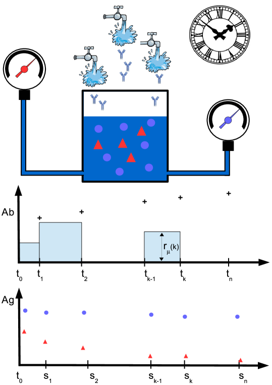
Figure 1: Immune Response: the Thought Experiment. Top drawing: antibodies (Abs) are released into a reservoir which contains a mixture of target antigen, Ag (red triangles) and self-antigen, self-Ag (blue circles). They can form Ab-Ag complexes and thereby reduce the amount of free (i.e. unbound) Abs, target Ag and self-Ag. The latter two amounts are measured, respectively, by the left and right ‘gauges’. The experiment is performed under constraints, such as finite duration and finite reservoir volume. Middle drawing: the release of antibodies is controlled by the flow rate (vertical axis) at any given time (horizontal axis). The total amount of Ab released up to time $t_{k}$ (crosses) is increasing with time. Bottom drawing: the amount of free target Ag (self-Ag) is decreasing with time. Each measurement is taken at the time-point $s_{k}$ with $s_{k}\gg t_{k}$, to ensure that the mixture in the reservoir is always in equilibrium.

Measurement protocol

The experimental measurement is defined by a set of time points $t_{0},\ldots,t_{k-1},t_{k},\ldots,t_{n}$ together with the flow rates $r_{\mu}(t_{1}),\ldots,r_{\mu}(t_{k-1}),r_{\mu}(t_{k}),\dots,r_{\mu}(t_{n})$ recorded at these times, for each Ab $\mu$ (see Figure 1). We label antibody types by Greek indices. The total amount of Ab $\mu$ released into the reservoir up to the time $t_{k}$ is given by the sum $b_{\mu}(t_{k})=\sum_{\ell=1}^{k}r_{\mu}(t_{\ell})(t_{\ell}-t_{\ell-1})$. If the flow rates $r_{\mu}(t)$ are smooth functions of time, each amount approaches an integral $b_{\mu}(t_{k})=\int_{t_{0}}^{t_{k}}r_{\mu}(t)\mathrm{d}t$ in the limit where the measurement times become arbitrarily close, $t_{\ell}-t_{\ell-1}\rightarrow 0$. The system in Figure 1 is then fully described by the amounts of Abs $\mathbf{b}(t)=(b_{1}(t),\dots,b_{M}(t))$, delivered into the reservoir up to time $t$, and the rates $\frac{\mathrm{d}}{\mathrm{d}t}\mathbf{b}(t)=\left(\frac{\mathrm{d}}{\mathrm{d}t}b_{1}(t),\dots,\frac{\mathrm{d}}{\mathrm{d}t}b_{M}(t)\right)$ of delivery of Abs. The amount of free target Ag, measured by the left gauge in Figure 1, is a function $A_{T}(\mathbf{b}(t))$ of the Abs $\mathbf{b}(t)$. The same is true for $A_{S}(\mathbf{b})$, the amount of free self-Ag, measured by the right gauge in the Figure 1. By construction, the total amount of free Ag in the experiment is a non-increasing function of time, i.e. $\frac{\mathrm{d}}{\mathrm{d}t}A_{T}\leq 0$ and $\frac{\mathrm{d}}{\mathrm{d}t}A_{S}\leq 0$.

Measurement of antibody affinity

Let the amount of free target Ag at time $t_{0}$ be $A_{T}(\mathbf{b}(t_{0}))$, and assume that at the next time-point $t_{1}$ we release into the reservoir a small amount $\Delta b_{\mu}$ of Ab $\mu$, i.e. $b_{\mu}(t_{1})=b_{\mu}(t_{0})+\Delta b_{\mu}$ and $b_{\nu}(t_{1})=b_{\nu}(t_{0})$ for all $\nu\neq\mu$. The resulting change in the amount of free target Ag is given by $\Delta A_{T}^{\mu}=A_{T}(\mathbf{b}(t_{1}))-A_{T}(\mathbf{b}(t_{0}))\leq 0$ and for $\Delta b_{\mu}\rightarrow 0$ we have $(\partial A_{T}/\partial b_{\mu})(\mathrm{d}b_{\mu}/\mathrm{d}t)\leq 0$. The same holds for the free self-Ag $A_{S}(\mathbf{b})$. Upon releasing a single Ab into the reservoir we will generally observe different behaviours of the gauges, which can be used to classify this Ab. Ab $\mu$ is more ‘reactive’ than Ab $\nu$ if $\Delta A_{T}^{\mu}\leq\Delta A_{T}^{\nu}$, for $\Delta b_{\mu}=\Delta b_{\nu}$, i.e. if the same amount of Ab reduces more Ag upon releasing type $\mu$ insterad of $\nu$ . Similarly, Ab $\mu$ is more self-reactive than Ab $\nu$ when $\Delta A_{S}^{\mu}\leq\Delta A_{S}^{\nu}$, and Ab $\mu$ is more reactive than self-reactive when $\Delta A_{T}^{\mu}\leq\Delta A_{S}^{\mu}$ (and vice versa). For $\Delta b_{\mu}\rightarrow 0$ all of the above definitions can implemented with partial derivatives, so Ab $\mu$ is more reactive than self-reactive when $(\partial A_{T}/\partial b_{\mu})\leq(\partial A_{S}/\partial b_{\mu})$, etc.

The difference $\Delta A_{T}^{\mu}$ is related to the affinity of Ab $\mu$ (22), which is usually defined as the ratio $r_{\mu}=K_{\mu}^{+}/K_{\mu}^{-}$ of forward/backward rates of the chemical reaction $Ag+Ab\rightleftharpoons AgAb$. In chemical equilibrium the latter can be computed experimentally, via the relation $r_{\mu}=[AgAb]/[Ag][Ab]$, upon measuring the amount $[Ag]$ of free target Ag, the amount $[Ab]$ of free Ab, and the amount $[AgAb]$ of Ag-Ab complexes, in the absence of other antibodies or antigens. In our notation, the affinity can be written as

$$r_{\mu}=-\frac{\left([Ag]\!-\![AgAb]\right)\!-\![Ag]}{[Ab]\!-\!0}\frac{1}{[Ag]}=-\frac{\Delta A_{T}^{\mu}}{\Delta b_{\mu}}\frac{1}{A_{T}(\mathbf{0})},$$ (1)

evaluated at $\mathbf{b}=\mathbf{0}$. Thus for $\Delta b_{\mu}\rightarrow 0$ it becomes the derivative

$$r_{\mu}(\mathbf{b}) = -\Big{(}\frac{\partial}{\partial b_{\mu}}\log A_{T}(\mathbf{b})\Big{)}_{\mathbf{b}=\mathbf{0}}.$$ (2)

For $\mathbf{b}\neq\mathbf{0}$, expression [2] can be seen as a generalised affinity, measured by adding a small amount of Ab $\mu$ in to the mixture of Ags and Abs. The affinity to self-Ag $r^{S}_{\mu}(\mathbf{b})$ uses the same definition as [2], but with $A_{S}(\mathbf{b})$ instead of $A_{T}(\mathbf{b})$.

In immunology one commonly thinks in terms of a repertoire of different antibodies, each reacting to target-Ag or to self-Ag, and of changing repertoires representing expansions of target-Ag antibodies in immune activation and deletion of self-Ag antibodies in immune tolerance. However, single antibodies can bind to multiple different antigens, with varying affinity, and these antigens could be either target-Ag or self-Ag. What we may have empirically determined to be a specific target-Ag binding antibody may in fact be a polyspecific antibody where the binding to self-Ag is so small as to be unnoticed. So we need to consider polyspecific antibodies, with variable affinities for binding to multiple Ag.

Using multiple antibody types to reduce free antigen

We assume here for simplicity that we have one type of target Ag, which we seek to reduce using a repertoire of antibodies. The Ag has $N_{A}$ distinct regions which can be ‘recognised’ by Abs, the epitopes. The Abs, represented by the amounts $\mathbf{b}=(b_{1},\ldots,b_{M})$, are assumed to interact with free epitopes, i.e. those not bound by Abs. The amounts of the free epitopes are written as $\boldsymbol{\mathcal{E}}=(\mathcal{E}_{1},\ldots,\mathcal{E}_{N_{A}})$. Each $\mathcal{E}_{i}\equiv\mathcal{E}_{i}(\mathbf{b})$ must be a non-decreasing function of the amount of Abs, such that $0\leq\mathcal{E}_{i}(\mathbf{b})\leq\mathcal{E}_{i}(\mathbf{0})$. Furthermore, the ‘amount’ of free target antigen $A_{T}(\mathbf{b})\equiv A_{T}\left(\boldsymbol{\mathcal{E}}\left(\mathbf{b}\right)\right)\geq 0$ will similarly be a non-decreasing function of the amount of free epitopes.

We assume that the protocol used to reduce the amount of Ag takes the form of differential equations for the rates of antibody delivery, given the amounts $\mathbf{b}\equiv\mathbf{b}(t)$ of Abs in the reservoir (as in biological processes), i.e. that

$$\frac{\mathrm{d}}{\mathrm{d}t}{b}_{\mu} = f_{\mu}\left(\mathbf{b}\right)$$ (3)

For the dynamics [3] to reduce target Ag, it is sufficient that the rate functions $f_{\mu}\!\left(\mathbf{b}\right)$ are positive,

$$\leavevmode\nobreak\ \leavevmode\nobreak\ \frac{\mathrm{d}}{\mathrm{d}t}A_{T}=\sum_{\mu=1}^{M}\frac{\partial A_{T}}{\partial b_{\mu}}\frac{\mathrm{d}}{\mathrm{d}t}{b}_{\mu}=-A_{T}(\mathbf{b})\!\!\sum_{\mu=1}^{M}r_{\mu}(\mathbf{b})f_{\mu}\left(\mathbf{b}\right)\leq 0.$$ (4)

Clearly, since $A_{T}(\mathbf{b})\geq 0$, the $A_{T}(\mathbf{b})$ is a Lyapunov function of [3]. The possible choices for the Ab delivery rate functions $f_{\mu}\!\left(\mathbf{b}\right)$ are further restricted by physical constraints in the experiment, such as finite time, finite volume, finite amount of available Abs, etc. Further complications occur if, in addition to target Ag, the reservoir also contains self Ag and, when we try to reduce free target Ag, only a finite amount of reduced self Ag (off-target damage) can be tolerated. It is natural to assume that the amount of free self Ag must depend in a similar way on the amount of free epitopes $\boldsymbol{\mathcal{E}}^{S}(\mathbf{b})=\left(\mathcal{E}_{1}^{S}(\mathbf{b}),\ldots,\mathcal{E}_{N_{S}}^{S}(\mathbf{b})\right)$ as the target antigen, so $A_{S}(\mathbf{b})=A_{S}\left(\boldsymbol{\mathcal{E}}^{S}(\mathbf{b})\right)$. Furthermore, one would expect that the Ab dynamics [3] is also a function of self-epitopes, i.e.

$$\frac{\mathrm{d}}{\mathrm{d}t}{b}_{\mu} = f_{\mu}\left(\boldsymbol{\mathcal{E}}(\mathbf{b}),\boldsymbol{\mathcal{E}}^{S}(\mathbf{b})\right)\!,$$ (5)

and that any biologically sensible choice $f_{\mu}(\ldots)$ must be an increasing function of $\boldsymbol{\mathcal{E}}(\mathbf{b})$ and a decreasing function of $\boldsymbol{\mathcal{E}}^{S}(\mathbf{b})$.

Antibody Dynamics

Principle of least damage

Instead of guessing an equation for the Ab delivery rates $f_{\mu}(\ldots)$, we take a Darwinian approach and assume that an optimized mechanism will have evolved that reduces the target Ag as quickly as possible, to minimise the ‘damage’ done, while minimising the harmful binding to self Ag in the process. The optimization problem can be solved using mathematical tools from physics. To this end we consider all possible paths $\mathbf{b}(t)$, allowed by the setup in Figure 1. Any such path will obey $\mathrm{d}b_{\mu}/\mathrm{d}t\geq 0$ and ${\mathrm{d}}A_{T}/\mathrm{d}t\leq 0$, i.e. each will minimize $A_{T}(\mathbf{b})$ (which we will call the ‘potential energy’). The latter is a property of the reservoir. We assume that the antibody delivery mechanism in Figure 1 has associated with it a ‘kinetic energy’ $\mathcal{T}(\mathrm{d}{\mathbf{b}}/\mathrm{d}t)$, which reflects the likely involvement of further variables governed by first order differential equations (equivalently, that the equations for $b_{\mu}$, if autonomous, will be at least second order). The path which begins at $\mathbf{b}(t_{0})$ at time $t_{0}$ and ends in $\mathbf{b}(t_{1})$ at time $t_{1}>t_{0}$, with $A_{T}(\mathbf{b}(t_{0}))\geq A_{T}(\mathbf{b}(t_{1}))$, can then be obtained (23) by minimising the action

$$\mathcal{S}\left(\mathbf{b},\frac{\mathrm{d}}{\mathrm{d}t}{\mathbf{b}}\right)=\int_{t_{0}}^{t_{1}}\!\mathrm{d}t\leavevmode\nobreak\ \mathcal{L}\left(\mathbf{b}(t),\frac{\mathrm{d}}{\mathrm{d}t}{\mathbf{b}}(t)\right),$$ (6)

where $\mathcal{L}\left(\mathbf{b},\frac{\mathrm{d}}{\mathrm{d}t}{\mathbf{b}}\right)=A_{T}(\mathbf{b})-\mathcal{T}(\frac{\mathrm{d}}{\mathrm{d}t}{\mathbf{b}})$ is the Lagrangian (see Materials and Methods).

Interpretation of the action

The area under the curve of $A_{T}(\mathbf{b}(t))$ on any path $\mathbf{b}(t)$, given by the integral

$$\mathcal{D}_{A}\left(t_{1}-t_{0}\right) = \int_{t_{0}}^{t_{1}}A_{T}(\mathbf{b}(t))\,\mathrm{d}t,$$ (7)

can be seen as a damage inflicted upon the organism during the time interval $[t_{0},t_{1}]$ by the presence of free target Ag. The intuition is that during any small time interval the damage inflicted by Ag is equal to the amount of free Ag times the time it spends in the organism. Definition [7] assumes moreover that this damage is cumulative, i.e. exposure to a large amount of Ag for a short time or a to a small amount of Ag for a longe time are equivalent. We observe that $0\leq\mathcal{D}_{A}\leq A_{T}(\mathbf{b}(t_{0}))\left(t_{1}-t_{0}\right)$, which follows from the properties $A_{T}(\mathbf{b}(t))\geq 0$ and $A_{T}(\mathbf{b}(t_{0}))\geq A_{T}(\mathbf{b}(t_{1}))$. So the path minimising the action [6] is the path which minimises the damage $\mathcal{D}_{A}\left(t_{1}-t_{0}\right)$, but subject to the constraint on $\mathrm{d}{\mathbf{b}}/\mathrm{d}t$ enforced by the term $\int_{t_{0}}^{t_{1}}\!\mathrm{d}t\leavevmode\nobreak\ \mathcal{T}\left(\frac{\mathrm{d}}{\mathrm{d}t}\mathbf{b}(t)\right)$ in the action (24).

Similar to [7], we can consider the integral

$$\mathcal{D}_{S}\left(t_{1}-t_{0}\right)=\int_{t_{0}}^{t_{1}}\!\mathrm{d}t\leavevmode\nobreak\ A_{S}(\mathbf{b}(t))\,,$$ (8)

where $0\leq\mathcal{D}_{S}\leq A_{S}(\mathbf{b}(t_{0}))\left(t_{1}-t_{0}\right)$. From this integral follows the ‘damage to self’, defined for each small time interval as the amount of free self Ag reduced by off-target action of the Abs times the duration of this reduction. Thus during the interval $[t_{0},t_{1}]$ this damage is $A_{S}(\mathbf{b}(t_{0}))\left(t_{1}-t_{0}\right)-\mathcal{D}_{S}\left(t_{1}-t_{0}\right)$.

Determination of optimal antibody dynamics

We minimise the action [6] subject to the constraint [8], i.e. we assume that removal of some amount of self Ag can be tolerated. This is equivalent (24) to minimisation of [6] with the Lagrangian

$$\mathcal{L}\left(\mathbf{b},\frac{\mathrm{d}}{\mathrm{d}t}{\mathbf{b}}\right)=A_{T}\left(\mathbf{b}\right)-\mathcal{T}\left(\frac{\mathrm{d}}{\mathrm{d}t}{\mathbf{b}}\right)-\gamma A_{S}(\mathbf{b}),$$ (9)

where $\gamma$ is a Lagrange parameter. The solution of the minimization is described by the Euler-Lagrange equation (see Materials and Methods):

$$\frac{\mathrm{d}}{\mathrm{d}t}\frac{\partial}{\partial(\mathrm{d}{b}_{\mu}/\mathrm{d}t)}\mathcal{T}\left(\frac{\mathrm{d}}{\mathrm{d}t}{\mathbf{b}}\right)=-\frac{\partial}{\partial b_{\mu}}\left[A_{T}(\mathbf{b})-\gamma A_{S}(\mathbf{b})\right].$$ (10)

We note that the above second order differential equations that describe the optimal control of antibody release were derived from general system level principles, with only minimal and plausible assumptions. Their solution will involve $2M$ constants, fixed by the boundary conditions $\mathbf{b}(t_{0})$ and $\mathbf{b}(t_{1})$.

The natural form for the kinetic energy is $\mathcal{T}(\mathrm{d}{\mathbf{b}}/\mathrm{d}t)=\frac{1}{2}\sum_{\mu=1}^{M}\Lambda_{\mu}(\mathrm{d}b_{\mu}/\mathrm{d}t)^{2}$, where $\Lambda_{\mu}>0$. It corresponds to assuming that at least one set of further (as yet unspecified) variables play a role in the Ab delivery process. Insertion into [10] gives us the ‘Newtonian’ equation

$$\Lambda_{\mu}\frac{\mathrm{d}^{2}}{\mathrm{d}t^{2}}{b}_{\mu}=A_{T}(\mathbf{b})\,r_{\mu}\!\left(\mathbf{b}\right)-\gamma A_{S}(\mathbf{b})\,r^{S}_{\mu}\!\left(\mathbf{b}\right),$$ (11)

where we used the affinities [2] to express the partial derivatives in [10]. We note that the $\Lambda_{\mu}$, which reflect properties of the Ab delivery mechanism, act to introduce ‘inertia’: large (small) $\Lambda_{\mu}$ reduce (increases) the tendency to change $\mathrm{d}{b}_{\mu}/\mathrm{d}t$. The total ‘force’ $\Lambda_{\mu}(\mathrm{d}^{2}{b}_{\mu}/\mathrm{d}t^{2})$ in [11] is a sum of a target Ag dependent term $A_{T}(\mathbf{b})\,r_{\mu}\!\left(\mathbf{b}\right)$ that increases the rate of Ab delivery, and a self Ag dependent term $-\gamma A_{S}(\mathbf{b})\,r^{S}_{\mu}\!\left(\mathbf{b}\right)$ which decreases Ab delivery (if $\gamma>0$). The state of mechanical equilibrium $\Lambda_{\mu}(\mathrm{d}^{2}{b}_{\mu}/\mathrm{d}t^{2})=0$, marking the balance of forces in [11], gives us, for $A_{S}(\mathbf{b}),r_{\mu}\!\left(\mathbf{b}\right)>0$, the identity

$$\frac{A_{T}(\mathbf{b})}{\gamma A_{S}(\mathbf{b})} = \frac{r^{S}_{\mu}\!\left(\mathbf{b}\right)}{r_{\mu}\!\left(\mathbf{b}\right)}.$$ (12)

It follows that there exists a function $\alpha(\mathbf{b})$ such that $r_{\mu}\!\left(\mathbf{b}\right)=\alpha(\mathbf{b})\,r^{S}_{\mu}\!\left(\mathbf{b}\right)$ for all $\mu$. Furthermore, for $\mathbf{b}=\mathbf{0}$ the latter gives us the relation $r_{\mu}=\alpha\,r^{S}_{\mu}$ between affinities, where $\alpha=\alpha(\mathbf{0})$.

Results

Free Ag reduced by large numbers of ‘weak’ antibodies

To proceed with our model we need to determine the dependencies of $A_{T}$ and $A_{S}$ on the antibody amounts $\mathbf{b}=(b_{1},\ldots,b_{M})$. Here we consider $M$ distinct univalent Abs ${\mathrm{I}}_{\mu}$, labelled by $\mu=1,\ldots,M$, each interacting with the univalent target Ag ($\triangle$) and self-Ag ($\circ$), via the following chemical reactions

$$\circ+{\mathrm{I}}_{\mu}\overset{{K_{\mu}^{S+}}}{\underset{{K_{\mu}^{S-}}}{\rightleftharpoons}}\overset{\circ}{\mathrm{I}}_{\mu}\leavevmode\nobreak\ \leavevmode\nobreak\ \leavevmode\nobreak\ \leavevmode\nobreak\ \leavevmode\nobreak\ \leavevmode\nobreak\ \leavevmode\nobreak\ \leavevmode\nobreak\ \triangle+{\mathrm{I}}_{\mu}\overset{K^{+}_{\mu}}{\underset{K^{-}_{\mu}}{\rightleftharpoons}}\overset{\triangle}{\mathrm{I}}_{\mu}$$ (13)

In chemical equilibrium, given the initial concentrations $A_{T}(\mathbf{0})$ of the target Ag and $A_{S}(\mathbf{0})$ of the self-Ag, the concentrations $A_{T}(\mathbf{b})$ of free target Ag and $A_{S}(\mathbf{b})$ of self-Ag are obtained by solving the following recursive system of equations; see Supplementary Information (SI), Section 1A:

$$A_{T} = \frac{A_{T}(\mathbf{0})}{1+\sum_{\mu=1}^{M}b_{\mu}\frac{r_{\mu}}{1+A_{T}\,r_{\mu}+A_{S}\,r^{S}_{\mu}}}$$ (14)

$$A_{S} = \frac{A_{S}(\mathbf{0})}{1+\sum_{\mu=1}^{M}b_{\mu}\frac{r^{S}_{\mu}}{1+A_{T}\,r_{\mu}+A_{S}\,r^{S}_{\mu}}}.$$ (15)

Each Ab is characterised by its affinities to the target Ag, $r_{\mu}=K_{\mu}^{+}/K_{\mu}^{-}$ (the ratio of forward and backward rates), and self-Ag, $r^{S}_{\mu}=K_{\mu}^{S+}/K_{\mu}^{S-}$. These give rise to the affinity vectors $\mathbf{r}=(r_{1},\ldots,r_{M})$ and $\mathbf{r}^{S}=(r_{1}^{S},\ldots,r_{M}^{S})$, which define the Ab repertoire. For multiple self-Ags the repertoire is a matrix of affinities (see SI, Sections 1A & 2A).

In order to use [11] one would prefer an explicit expression for $A_{T}\!\left(\mathbf{b}\right)$ and $A_{S}\!\left(\mathbf{b}\right)$, but how to solve the non-linear recursion [14] analytically is not clear. However, if we assume that affinities scale as $r_{\mu}\equiv r_{\mu}/M$ and $r_{\mu}^{S}\equiv r_{\mu}^{S}/M$, then in the regime $M\rightarrow\infty$ of having a large number of individually weak Abs, we obtain the concentrations of free Ags in explicit form (see Materials and Methods):

$$A_{T}\left(\mathbf{b}\right)=\frac{A_{T}(\mathbf{0})}{1+B(\mathbf{b})},\leavevmode\nobreak\ \leavevmode\nobreak\ \leavevmode\nobreak\ \leavevmode\nobreak\ \leavevmode\nobreak\ \leavevmode\nobreak\ \leavevmode\nobreak\ \leavevmode\nobreak\ A_{S}\left(\mathbf{b}\right)=\frac{A_{S}(\mathbf{0})}{1+B_{S}(\mathbf{b})}$$ (16)

expressed as functions of the averages

$$B_{T}(\mathbf{b})=\frac{1}{M}\sum_{\mu=1}^{M}r_{\mu}\,b_{\mu},\leavevmode\nobreak\ \leavevmode\nobreak\ \leavevmode\nobreak\ \leavevmode\nobreak\ \leavevmode\nobreak\ \leavevmode\nobreak\ B_{S}(\mathbf{b})=\frac{1}{M}\sum_{\mu=1}^{M}r^{S}_{\mu}\,b_{\mu}.$$

The averages $B_{T}(\mathbf{b})$ and $B_{S}(\mathbf{b})$ can be seen as total affinities to the target Ag and the self Ag. A similar object, where $b_{\mu}$ was the number of B cells with affinity to Ag $r_{\mu}/M$, was postulated as an ‘energy’ function of somatic hypermutation in (14).

We note that the result [16], although derived for univalent Abs and Ag, is also true for multivalent Abs (see SI, Section 1B). Thus our model predicts that it is possible to reduce target antigen without requiring affinity-matured antibodies, such as those produced in a T-dependent reaction, if a sufficient number of weaker binders are available. Furthermore, the framework outlined here can easily incorporate multiple Ags, chemical species binding Ab-Ag complexes, phagocytes, etc. (see SI, Section 1A)

Reduced macroscopic description

Let us consider the Euler-Lagrange equations [11] for the free and self-Ag. Via [16], and upon reverting from the right-hand side of [11] back to that of its predecessor [10], these now take the form

$$\Lambda_{\mu}\frac{\mathrm{d}^{2}}{\mathrm{d}t^{2}}{b}_{\mu}=\frac{A_{T}(\mathbf{0})}{\left(1+B_{T}\right)^{2}}\frac{r_{\mu}}{M}-\gamma\frac{A_{S}(\mathbf{0})}{\left(1+B_{S}\right)^{2}}\frac{r^{S}_{\mu}}{M},$$ (17)

where $B_{T}\equiv B(\mathbf{b})$ and $B_{S}\equiv B_{S}(\mathbf{b})$. If we assume that $\Lambda_{\mu}$ scales as $\Lambda_{\mu}=\lambda_{\mu}\phi(M)/M$, where $\phi(M)=o(M)$, we can derive for $M\to\infty$ the following equations (SI, Section 2A):

$$\frac{\mathrm{d}^{2}}{\mathrm{d}t^{2}}{B}_{T} = \frac{A_{0}^{T}|\mathbf{r}|^{2}}{\left(1+B_{T}\right)^{2}}-\gamma\frac{A_{0}^{S}(\mathbf{r}\cdot\mathbf{r}^{S})}{\left(1+B_{S}\right)^{2}}$$ (18)

$$\frac{\mathrm{d}^{2}}{\mathrm{d}t^{2}}{B}_{S} = \frac{A_{0}^{T}(\mathbf{r}\cdot\mathbf{r}^{S})}{\left(1+B_{T}\right)^{2}}-\gamma\frac{A_{0}^{S}|\mathbf{r}^{S}|^{2}}{\left(1+B_{S}\right)^{2}},$$

where in the above we used the dot product definition $\mathbf{x}\cdot\mathbf{y}=M^{-1}\sum_{\mu=1}^{M}\lambda_{\mu}^{-1}x_{\mu}y_{\mu}$, with the associated norm $|\mathbf{x}|=\sqrt{\mathbf{x}\cdot\mathbf{x}}$. We assume that at time $t=0$ all Ab amounts and production rates are zero, i.e. $b_{\mu}=\mathrm{d}{b}_{\mu}/\mathrm{d}t=0$ for all $\mu$, so the initial conditions for [18] are $B_{T}(0)=B_{S}(0)=0$ and $(\mathrm{d}{B}_{T}/\mathrm{d}t)(0)=(\mathrm{d}{B}_{S}/\mathrm{d}t)(0)=0$. Furthermore, the average Ab concentration $\tilde{B}(t)=M^{-1}\sum_{\nu=1}^{M}b_{\nu}(t)$ is governed by the equation

$$\frac{\mathrm{d}^{2}}{\mathrm{d}t^{2}}{\tilde{B}} = \frac{A_{0}^{T}(\mathbf{r}\cdot\mathbf{1})}{\left(1+B_{T}\right)^{2}}-\gamma\frac{A_{0}^{S}(\mathbf{r}^{S}\!\cdot\mathbf{1})}{\left(1+B_{S}\right)^{2}}.$$ (19)

with the short-hand $\mathbf{1}=(1,\ldots,1)$.

The simplest case to consider is that where each Ab is either self-reactive or non-self-reactive, i.e. for each $\mu$ either $r_{\mu}>0$ or $r^{S}_{\mu}>0$, but never both. This implies that $\mathbf{r}\cdot\mathbf{r}^{S}=0$, and that hence [18] decouples into two independent equations:

$$\frac{\mathrm{d}^{2}}{\mathrm{d}t^{2}}{B}_{T}=\frac{A_{0}^{T}|\mathbf{r}|^{2}}{\left(1+B_{T}\right)^{2}},\leavevmode\nobreak\ \leavevmode\nobreak\ \leavevmode\nobreak\ \leavevmode\nobreak\ \leavevmode\nobreak\ \leavevmode\nobreak\ \frac{\mathrm{d}^{2}}{\mathrm{d}t^{2}}{B}_{S}=-\gamma\frac{A_{0}^{S}|\mathbf{r}^{S}|^{2}}{\left(1+B_{S}\right)^{2}}$$ (20)

The dynamics of $B_{T}$ is now conservative, with energy function

$$E\Big{(}B_{T},\frac{\mathrm{d}B_{T}}{\mathrm{d}t}\Big{)}=\frac{1}{2|\mathbf{r}|^{2}}\Big{(}\frac{\mathrm{d}B_{T}}{\mathrm{d}t}\Big{)}^{2}+\frac{A_{0}^{T}}{1+B_{T}},$$ (21)

where the terms $(\mathrm{d}B_{T}/\mathrm{d}t)^{2}/2|\mathbf{r}|^{2}$ and $A_{0}^{T}/(1+B_{T})$ are, respectively, the ‘kinetic’ and ‘potential’ energies. The equation for $B_{T}$ describes the motion of a ‘particle’ of ‘mass’ $1/|\mathbf{r}|^{2}$ in in a potential field (23). Furthermore, solving the energy conservation equation $E(B_{T},\mathrm{d}B_{T}/\mathrm{d}t)=E(B_{T}(0),(\mathrm{d}B_{T}/\mathrm{d}t)(0))$, for $B(0)=(\mathrm{d}B_{T}/\mathrm{d}t)(0)=0$, gives us

$$\frac{\mathrm{d}}{\mathrm{d}t}{B_{T}} = \sqrt{2A_{0}^{T}|\mathbf{r}|^{2}\frac{B_{T}}{\left(1+B_{T}\right)}}.$$ (22)

The function $\sqrt{B_{T}/(1+B_{T})}\in[0,1]$ is monotonic increasing and concave for $B_{T}\geq 0$. Hence t $B(t)$ is bounded from above by $\sqrt{2A_{0}^{T}|\mathbf{r}|^{2}}\,t$ and this bound is saturated as $t\rightarrow\infty$. Also, the (normalised) amount of target antigen $A_{T}(\mathbf{b}(t))/A_{T}(\mathbf{0})=(1+B_{T}(t))^{-1}$ is bounded from below by $(1+\sqrt{2A_{0}^{T}|\mathbf{r}|^{2}}\,t)^{-1}$.

In a similar manner we simplify the dynamics of $B_{S}$, which is also conservative, describing the motion of a particle of mass $|\mathbf{r}^{S}|^{-2}$ and potential energy $-\gamma A_{0}^{S}/(1+B_{S})$. Here we find

$$\Big{(}\frac{\mathrm{d}}{\mathrm{d}t}{B}_{S}\Big{)}^{2}=-2\gamma A_{0}^{S}|\mathbf{r}^{S}|^{2}\frac{B_{S}}{\left(1+B_{S}\right)}$$ (23)

Since $\gamma>0$ and with the assumed initial conditions, the (trivial) solution is $B_{S}=0$, i.e. self-reactive Abs are not used.

We have now seen that [20] can be mapped into equations of Classical Mechanics. The equation for $B_{S}$ describes the acceleration of a particle of mass $|\mathbf{r}^{S}|^{-2}$ in a gravitational field with gravitational constant $\gamma$, created by a another particle of mass $A_{0}^{S}$ and radius one (23). The equation for $B_{T}$ has a similar interpretation but with a repulsive potential.

Ag removal is faster in a more diverse repertoire, and slower when the repertoire has higher self-reactivity

We return to the more general case where $\mathbf{r}\cdot\mathbf{r}^{S}>0$, so Abs may have the potential to bind both target Ag and self Ag. Further analytic results can be obtained in the equilibrium regime of [18], defined by $\mathrm{d}^{2}B_{T}/\mathrm{d}t^{2}=\mathrm{d}^{2}B_{S}/\mathrm{d}t^{2}=0$. This can only occur when $r_{\mu}=\alpha r^{S}_{\mu}$ for all $\mu$ (see SI, Section 2B) , where $\alpha>0$. The inverse $\alpha^{-1}$ can be seen as a degree of self-reactivity. From [Free Ag reduced by large numbers of ‘weak’ antibodies] it follows that $B_{T}=\alpha B_{S}$ in this regime, and that [18] can be reduced to a single equation:

$$\frac{\mathrm{d}^{2}}{\mathrm{d}t^{2}}{B}_{S}=A_{0}^{S}|\mathbf{r}^{S}|^{2}\left[\frac{\alpha\beta}{\left(1+\alpha B_{S}\right)^{2}}-\frac{\gamma}{\left(1+B_{S}\right)^{2}}\right],$$ (24)

with $\beta=A_{0}^{T}/A_{0}^{S}$. It is easy to show, using the above equation and [19], that now $\mathrm{d}^{2}\tilde{B}/\mathrm{d}t^{2}=(\mathbf{r}^{S}\!\cdot\mathbf{1})|\mathbf{r}^{S}|^{-2}\mathrm{d}^{2}{B}_{S}/\mathrm{d}t^{2}$, and hence the average concentration of Abs is given by

$$\tilde{B}=(\mathbf{r}^{S}\!\cdot\mathbf{1})|\mathbf{r}^{S}|^{-2}B_{S}.$$ (25)

The dynamics [24] is again conservative, now with energy

$$E\Big{(}B_{S},\frac{\mathrm{d}{B}_{S}}{\mathrm{d}t}\Big{)}=\frac{1}{2|\mathbf{r}^{S}|^{2}}\Big{(}\frac{\mathrm{d}{B_{S}}}{\mathrm{d}t}\Big{)}^{2}+\frac{\beta A_{0}^{S}}{1+\alpha B_{S}}-\frac{\gamma A_{0}^{S}}{1+B_{S}}.$$ (26)

As before we can use energy conservation, following initial conditions $B_{S}(0)=(\mathrm{d}B_{S}/\mathrm{d}t)(0)=0$, to derive

$$\frac{\mathrm{d}}{\mathrm{d}t}{B}_{S}=\sqrt{\!2A_{0}^{S}|\mathbf{r}^{S}|^{2}\!\left(\frac{\beta\alpha B_{S}}{1+\alpha B_{S}}-\frac{\gamma B_{S}}{1+B_{S}}\right)}.$$ (27)

From this follows the following upper bound, which is saturated as $t\to\infty$ (see SI, Section 2B):

$$B_{S}(t)\leq t/\tau,$$ (28)

with the time constant

$$\tau=1/|\mathbf{r}^{S}|\sqrt{2A_{0}^{S}(\beta-\gamma)}.$$ (29)

As a consequence of [28], we find for the normalised target Ag

$$\frac{A_{T}(\mathbf{b}(t))}{A_{T}(\mathbf{0})}=\frac{1}{1+\alpha B_{S}(t)}\geq\frac{1}{1+\alpha t/\tau}.$$ (30)

So $\tau/\alpha$ is a lower bound for the half-life of free target Ag; to achieve $A_{T}(\mathbf{b}(t))/A_{T}(\mathbf{0})=\frac{1}{2}$, the required time $t$ has to be at least $\tau/\alpha$. The lower bound for the half-life of self-Ag, derived by a similar argument, is found to be $\tau$. Furthermore, if we define $w(\boldsymbol{\lambda})=M^{-1}\sum_{\mu=1}^{M}\lambda^{-1}_{\mu}$ then

$$|\mathbf{r}^{S}|=\sqrt{w(\boldsymbol{\lambda})\left[\sigma_{\boldsymbol{\lambda}}^{2}\left(\mathbf{r}^{S}\right)+m_{\boldsymbol{\lambda}}^{2}\left(\mathbf{r}^{S}\right)\right]},$$ (31)

where $\sigma_{\boldsymbol{\lambda}}^{2}\left(\mathbf{r}^{S}\right)=|\mathbf{r}^{S}|^{2}/w(\boldsymbol{\lambda})-((\mathbf{r}^{S}\!\cdot\mathbf{1})/w(\boldsymbol{\lambda}))^{2}$and $m_{\boldsymbol{\lambda}}(\mathbf{r}^{S})=(\mathbf{r}^{S}\!\cdot\mathbf{1})/w(\boldsymbol{\lambda})$ are, respectively, variance and mean of the self-affinities $\mathbf{r}^{S}$ (see SI, Section 2B). Thus $\tau$ is monotonically decreasing with the variance $\sigma_{\boldsymbol{\lambda}}^{2}(\mathbf{r}^{S})$ and the mean $m_{\boldsymbol{\lambda}}(\mathbf{r}^{S})$. Since the former can be seen as a measure of the repertoire’s ‘diversity’, having a more diverse repertoire facilitates a more rapid reduction of target Ag.

We also solved the differential equation [24] numerically for different inverse self-reactivities $\alpha$. The solutions are plotted in Supplementary Information, in Figures 5-8. Comparison of the upper bound [28] with the solutions of [24] in Figure 9 allows us to summarise various regimes. We first define, using [7], the normalised damage per unit time $\delta_{A}(t_{1}-t_{0})=\mathcal{D}_{A}\left(t_{1}-t_{0}\right)/A_{T}(\mathbf{b}(t_{0}))\left(t_{1}-t_{0}\right)$, where $0\leq\delta_{A}\leq 1$, and, using [8], the normalised damage to self per unit time $1-\delta_{S}(t_{1}-t_{0})=1-\mathcal{D}_{S}\left(t_{1}-t_{0}\right)/A_{S}(\mathbf{b}(t_{0}))\left(t_{1}-t_{0}\right)$, where $0\leq\delta_{S}\leq 1$ and $0\leq 1-\delta_{S}\leq 1$. For the system [16], on the time interval $[0,t]$, the above definitions give us

$$\delta_{A}(t)=\frac{1}{t}\int_{0}^{t}\!\frac{\mathrm{d}t^{\prime}}{1+\alpha B_{S}({t^{\prime}})},\leavevmode\nobreak\ \leavevmode\nobreak\ \leavevmode\nobreak\ \leavevmode\nobreak\ \delta_{S}(t)=\frac{1}{t}\int_{0}^{t}\!\frac{\mathrm{d}t^{\prime}}{1+\!B_{S}({t^{\prime}})}$$ (32)

Now since $(1+\alpha B_{S})^{-1}$ is a monotonic decreasing function of $B_{S}$, the upper bound [28] gives us the lower bounds

$$\delta_{A}(t) \geq \frac{\tau}{\alpha\,t}\log\left(1+\frac{\alpha\,t}{\tau}\right)$$ (33)

$$\delta_{S}(t) \geq \frac{\tau}{t}\log\left(1+\frac{t}{\tau}\right).$$ (34)

The latter gives us the upper bound $1-(\tau/t)\log(1+t/\tau)\geq 1-\delta_{S}(t)$ for the damage to self.

The two bounds on damages are plotted in Figure 2 for different values of self-reactivity constant $\alpha$. For a repertoire with Abs binding $\alpha$ times stronger to the target Ag than to the self-Ag the immune response is ‘normal’ and ‘autoimmune’, respectively, when $\alpha>1$ and $\alpha<1$. The normal response is characterised by a large decrease of free target Ag and a small decrease in free self-Ag per unit of time. For the autoimmune response it is the opposite. Furthermore, the normal response is ‘accelerated’ by a larger $\alpha$ and increased repertoire diversity, but, for the same repertoire diversity, the autoimmune response is slower.

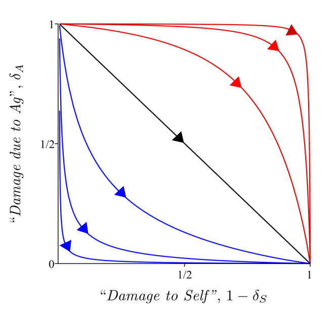
Figure 2: The damage due to antigen $\delta_{A}$ (lower bound), plotted as a function of the damage to self $1-\delta_{S}$ (upper bound) for the inverse self-reactivity $\alpha=\{10^{-3},10^{-2},10^{-1}\}$ (top red curves with $\alpha$ increasing from top to bottom) , $\alpha=1$ (black line) and $\alpha=\{10,10^{2},10^{3}\}$ (bottom blue curves with $\alpha$ increasing from top to bottom). The direction of ‘time’ $t/\tau\in[0,\infty)$, indicated by arrows, is always from left to right.

Discussion

In this work we have shown, using only minimal assumptions, that antibody repertoire diversity is important in the effective removal of antigen, in multiple ways. Not just because the repertoire will then have more chance of containing a single dominant antibody that can react to the target-Ag, but also because for a more diverse repertoire the half life of target-Ag will be smaller. Hence any decrease in repertoire diversity, such as that observed in older age, or caused by a prior immune response, can have an adverse effect on the immune response to challenge. Furthermore, reduction in efficacy of central tolerance mechanisms such as can occur in older age, will result in greater self-reactivity in the repertoire, and this too will hamper an efficient immune response against target-Ag.

The mathematical framework in the form developed here can for now only be used to model the immune response to a finite amount of Ag, with a fixed repertoire of Abs. Adaptation of the affinities of Abs to target Ag via affinity maturation (22) is not yet included. To model the latter on could modify the Lagrangian [9], and derive dynamic equations for affinities. Also the present restriction on the amount of Ag can be relaxed within the current framework, by introducing (partially stochastic) Ag reproduction and death.

The Variational Problem

We aim to find the path $\mathbf{b}(t)$ that minimises the action [6] on the time-interval $[t_{0},t_{1}]$ with the boundaries $\mathbf{b}(t_{0})=\mathbf{b}_{0}$ and $\mathbf{b}(t_{1})=\mathbf{b}_{1}$. This path must solve the equation $\delta\mathcal{S}=0$ for the difference $\delta\mathcal{S}=\mathcal{S}(\mathbf{b}+\delta\mathbf{b},\mathrm{d}{\mathbf{b}}/\mathrm{d}t+\mathrm{d}\delta{\mathbf{b}}/\mathrm{d}t)-\mathcal{S}(\mathbf{b},\mathrm{d}{\mathbf{b}}/\mathrm{d}t)$, where $\mathbf{b}(t)+\delta\mathbf{b}(t)$ is any perturbed path with $\delta\mathbf{b}(t_{0})=\delta\mathbf{b}(t_{1})=0$ (24). Using the differential operator $\nabla_{\mathbf{b}}=\left(\partial/\partial b_{1},\ldots,\partial/\partial b_{M}\right)$ this difference, up to the order $O\!\left({|\delta\mathbf{b}|}^{2}\right)$, can be written in the form

$$\delta\mathcal{S} = \int_{t_{0}}^{t_{1}}\mathcal{L}\left(\mathbf{b}\!+\!\delta\mathbf{b},\frac{\mathrm{d}{\mathbf{b}}}{\mathrm{d}t}\!+\!\delta\frac{\mathrm{d}{\mathbf{b}}}{\mathrm{d}t}\right)\,\mathrm{d}t-\!\int_{t_{0}}^{t_{1}}\mathcal{L}\left(\mathbf{b},\frac{\mathrm{d}{\mathbf{b}}}{\mathrm{d}t}\right)\,\mathrm{d}t$$

$$= \int_{t_{0}}^{t_{1}}\!\!\!\!\left\{\delta\mathbf{b}.\nabla_{\mathbf{b}}\mathcal{L}\left(\mathbf{b},\frac{\mathrm{d}{\mathbf{b}}}{\mathrm{d}t}\right)+\delta\frac{\mathrm{d}{\mathbf{b}}}{\mathrm{d}t}.\nabla_{\mathrm{d}\mathbf{b}/\mathrm{d}t}\mathcal{L}\left(\mathbf{b},\frac{\mathrm{d}{\mathbf{b}}}{\mathrm{d}t}\right)\right\}\!\mathrm{d}t$$

$$= \left[\delta\mathbf{b}\,.\nabla_{\mathrm{d}\mathbf{b}/\mathrm{d}t}\mathcal{L}\left(\mathbf{b},\frac{\mathrm{d}{\mathbf{b}}}{\mathrm{d}t}\right)\right]_{t_{0}}^{t_{1}}+\cdots$$

$$\cdots+\int_{t_{0}}^{t_{1}}\delta\mathbf{b}\,.\Big{\{}\nabla_{\mathbf{b}}\mathcal{L}\left(\mathbf{b},\frac{\mathrm{d}{\mathbf{b}}}{\mathrm{d}t}\right)-\frac{\mathrm{d}}{\mathrm{d}t}\nabla_{\mathrm{d}\mathbf{b}/\mathrm{d}t}\mathcal{L}\left(\mathbf{b},\frac{\mathrm{d}{\mathbf{b}}}{\mathrm{d}t}\right)\Big{\}}\mathrm{d}t$$

$$= \int_{t_{0}}^{t_{1}}\delta\mathbf{b}\,.\!\left\{\nabla_{\mathbf{b}}\mathcal{L}\left(\mathbf{b},\frac{\mathrm{d}{\mathbf{b}}}{\mathrm{d}t}\right)-\frac{\mathrm{d}}{\mathrm{d}t}\nabla_{\mathrm{d}\mathbf{b}/\mathrm{d}t}\mathcal{L}\left(\mathbf{b},\frac{\mathrm{d}{\mathbf{b}}}{\mathrm{d}t}\right)\right\}\mathrm{d}t$$

where we used integration by parts and the stated boundary conditions. Solving $\delta\mathcal{S}=0$ for the part of $\delta\mathcal{S}$ that is linear in $\delta\mathbf{b}$ gives us the so-called Euler-Lagrange equation

$$\frac{\mathrm{d}}{\mathrm{d}t}\nabla_{\left(\mathrm{d}{\mathbf{b}}/\mathrm{d}t\right)}\mathcal{L}\left(\mathbf{b},\frac{\mathrm{d}{\mathbf{b}}}{\mathrm{d}t}\right)=\nabla_{\mathbf{b}}\mathcal{L}\left(\mathbf{b},\frac{\mathrm{d}{\mathbf{b}}}{\mathrm{d}t}\right)$$ (36)

with boundary conditions $\mathbf{b}(t_{0})=\mathbf{b}_{0}$ and $\mathbf{b}(t_{1})=\mathbf{b}_{1}$.

Mean-Field Limit

Here we explain briefly the derivation of [16] from [14]. Substituting $r_{\mu}\to r_{\mu}/M$ and $r^{S}_{\mu}\to r^{S}_{\mu}/M$ into [14] gives

$$\frac{A_{T}}{A_{T}(\mathbf{0})}=\frac{1}{1+\frac{1}{M}\sum_{\mu=1}^{M}r_{\mu}b_{\mu}(1+A_{T}\,r_{\mu}/M+A_{S}\,r^{S}_{\mu}/M)^{-1}}$$ (37)

hence, if $A_{T}(\mathbf{0})=\phi(M)A_{0}^{T}$ and $A_{S}(\mathbf{0})=\phi(M)A_{0}^{S}$, where $\phi(M)=o(M)$, i.e. $\lim_{M\rightarrow\infty}\phi(M)/M=0$, then for $M\to\infty$ we will indeed find the mean-field expressiom [16] since

$$\frac{A_{T}}{A_{T}(\mathbf{0})}=\frac{1}{1+\frac{1}{M}\sum_{\mu=1}^{M}r_{\mu}b_{\mu}+O(\phi(M)/M)}$$ (38)

This work was supported by the Medical Research Council of the United Kingdom (grant MR/L01257X/1). A.M. would like to thank Adriano Barra, Alessia Annibale, Fabián Aguirre López, Attila Csikász-Nagy and Martí Aldea Malo for very enlightening discussions.

Supplementary Information

1 Chemical kinetics of antigen-antibody reactions

1.1 Univalent antibodies reacting with univalent antigens

We consider $M$ different univalent antibodies (Abs), represented by the symbols ${\mathrm{I}}_{\mu}$ with $\mu\in\{1,\ldots,M\}$, forming complexes with $M_{A}$ different univalent target antigens (Ags), $\triangle_{v}$ with $v\in\{1,\ldots,M_{A}\}$, and $M_{S}$ self-Ags, $\circ_{u}$ with $u\in\{1,\ldots,M_{S}\}$. The Ag bound by Ab $\overset{\triangle_{v}}{\mathrm{I}_{\mu}}$ and $\overset{\circ_{u}}{\mathrm{I}_{\mu}}$ will subsequently form complexes with ‘phagocytic’ species $\mathrm{P}$ (22). The formation and dissociation of complexes is modelled by the four chemical reactions

$$\circ_{u}+{\mathrm{I}}_{\mu}\overset{{K_{\mu u}^{S+}}}{\underset{{K_{\mu u}^{S-}}}{\rightleftharpoons}}\leavevmode\nobreak\ \overset{\circ_{u}}{\mathrm{I}_{\mu}}\leavevmode\nobreak\ \leavevmode\nobreak\ \leavevmode\nobreak\ \leavevmode\nobreak\ \leavevmode\nobreak\ \leavevmode\nobreak\ \leavevmode\nobreak\ \leavevmode\nobreak\ \leavevmode\nobreak\ \leavevmode\nobreak\ \overset{\circ_{u}}{\mathrm{I}_{\mu}}+\mathrm{P}\overset{K^{+}}{\underset{K^{-}}{\rightleftharpoons}}\leavevmode\nobreak\ \overset{\circ_{u}}{\mathrm{I}_{\mu}}\mathrm{P}\leavevmode\nobreak\ \leavevmode\nobreak\ \leavevmode\nobreak\ \leavevmode\nobreak\ \leavevmode\nobreak\ \leavevmode\nobreak\ \leavevmode\nobreak\ \leavevmode\nobreak\ \leavevmode\nobreak\ \leavevmode\nobreak\ \triangle_{v}+{\mathrm{I}}_{\mu}\overset{K^{+}_{\mu v}}{\underset{K^{-}_{\mu v}}{\rightleftharpoons}}\leavevmode\nobreak\ \overset{\triangle_{v}}{\mathrm{I}_{\mu}}\leavevmode\nobreak\ \leavevmode\nobreak\ \leavevmode\nobreak\ \leavevmode\nobreak\ \leavevmode\nobreak\ \leavevmode\nobreak\ \leavevmode\nobreak\ \leavevmode\nobreak\ \leavevmode\nobreak\ \leavevmode\nobreak\ \overset{\triangle_{v}}{\mathrm{I}_{\mu}}+\mathrm{P}\overset{K^{+}}{\underset{K^{-}}{\rightleftharpoons}}\leavevmode\nobreak\ \overset{\triangle_{v}}{\mathrm{I}_{\mu}}\mathrm{P}.$$ (39)

In chemical equilibrium (25) the concentrations of free self-Ag, target Ag, Ab and P (denoted, respectively, by the symbols $\left[\circ_{u}\right]$, $\left[\triangle_{v}\right]$, $\left[\mathrm{I}_{\mu}\right]$ and $\left[\mathrm{P}\right]$) are related to the concentration of bound species $\overset{\circ_{u}}{\mathrm{I}_{\mu}}$, $\overset{\circ_{u}}{\mathrm{I}_{\mu}}\mathrm{P}$, $\overset{\triangle_{v}}{\mathrm{I}_{\mu}}$ and $\overset{\triangle_{v}}{\mathrm{I}_{\mu}}\mathrm{P}$ (denoted, respectively, by the symbols $[\overset{\circ_{u}}{\mathrm{I}_{\mu}}]$, $[\overset{\circ_{u}}{\mathrm{I}_{\mu}}\mathrm{P}]$, $[\overset{\triangle_{v}}{\mathrm{I}_{\mu}}]$ and $[\overset{\triangle_{v}}{\mathrm{I}_{\mu}}\mathrm{P}]$) via the affinity parameters $r_{\mu u}^{S}={K_{\mu u}^{S+}}/{K_{\mu u}^{S-}}$, $r_{\mu v}={K^{+}_{\mu v}}{K^{-}_{\mu v}}$ and $r=K^{+}/K^{-}$, i.e. the ratios of forward/backward rates of reactions:

$$r_{\mu u}^{S}=\frac{[\overset{\circ_{u}}{\mathrm{I}_{\mu}}]}{\left[\circ_{u}\right]\left[\mathrm{I}_{\mu}\right]}\leavevmode\nobreak\ \leavevmode\nobreak\ \leavevmode\nobreak\ \leavevmode\nobreak\ \leavevmode\nobreak\ \leavevmode\nobreak\ \leavevmode\nobreak\ \leavevmode\nobreak\ r=\frac{[{\overset{\circ_{u}}{\mathrm{I}_{\mu}}}\mathrm{P}]}{[\overset{\circ_{u}}{\mathrm{I}_{\mu}}]\left[\mathrm{P}\right]}\leavevmode\nobreak\ \leavevmode\nobreak\ \leavevmode\nobreak\ \leavevmode\nobreak\ \leavevmode\nobreak\ \leavevmode\nobreak\ \leavevmode\nobreak\ \leavevmode\nobreak\ r_{\mu v}=\frac{[\overset{\triangle_{v}}{\mathrm{I}_{\mu}}]}{\left[\triangle_{v}\right]\left[\mathrm{I}_{\mu}\right]}\leavevmode\nobreak\ \leavevmode\nobreak\ \leavevmode\nobreak\ \leavevmode\nobreak\ \leavevmode\nobreak\ \leavevmode\nobreak\ \leavevmode\nobreak\ \leavevmode\nobreak\ r=\frac{[\overset{\triangle_{v}}{\mathrm{I}_{\mu}}\mathrm{P}]}{[\overset{\triangle_{v}}{\mathrm{I}_{\mu}}]\left[\mathrm{P}\right]}$$ (40)

Upon denoting the initial concentrations of the species $\circ_{u}$, $\triangle_{v}$, $\mathrm{I}_{\mu}$ and $\mathrm{P}$ by $\left[\circ_{u}\right]_{0}$, $\left[\triangle_{v}\right]_{0}$, $\left[\mathrm{I}_{\mu}\right]_{0}$ and $\left[\mathrm{P}\right]_{0}$, we can use mass conservation to write

$$\left[\circ_{u}\right]_{0} = \left[\circ_{u}\right]+\sum_{\mu=1}^{M}\,[\overset{\circ_{u}}{\mathrm{I}_{\mu}}]+\sum_{\mu=1}^{M}\,[\overset{\circ_{u}}{\mathrm{I}_{\mu}}\mathrm{P}]$$ (41)

$$\left[\triangle_{v}\right]_{0} = \left[\triangle_{v}\right]+\sum_{\mu=1}^{M}\,[\overset{\triangle_{v}}{\mathrm{I}_{\mu}}]+\sum_{\mu=1}^{M}\,[\overset{\triangle_{v}}{\mathrm{I}_{\mu}}\mathrm{P}]$$ (42)

$$\left[\mathrm{I}_{\mu}\right]_{0} = \left[\mathrm{I}_{\mu}\right]+\sum_{u=1}^{M_{S}}\,[\overset{\circ_{u}}{\mathrm{I}_{\mu}}]+\sum_{v=1}^{M_{A}}\,[\overset{\triangle_{v}}{\mathrm{I}_{\mu}}]+\sum_{u=1}^{M_{S}}\,[\overset{\circ_{u}}{\mathrm{I}_{\mu}}\mathrm{P}]+\sum_{v=1}^{M_{A}}\,[\overset{\triangle_{v}}{\mathrm{I}_{\mu}}\mathrm{P}]$$ (43)

$$\left[\mathrm{P}\right]_{0} = \left[\mathrm{P}\right]+\sum_{\mu=1}^{M}\sum_{u=1}^{M_{S}}\,[\overset{\circ_{u}}{\mathrm{I}_{\mu}}\mathrm{P}]+\sum_{\mu=1}^{M}\sum_{v=1}^{M_{A}}\,[\overset{\triangle_{v}}{\mathrm{I}_{\mu}}\mathrm{P}]$$ (44)

By using [40] these expressions can be written in the alternative form

$$\left[\circ_{u}\right]_{0} = \left[\circ_{u}\right]\Big{(}1+\left(1+r[\mathrm{P}]\right)\sum_{\mu=1}^{M}r_{\mu u}^{S}[{\mathrm{I}}_{\mu}]\Big{)}$$ (45)

$$\left[\triangle_{v}\right]_{0} = \left[\triangle_{v}\right]\Big{(}1+\left(1+r[\mathrm{P}]\right)\sum_{\mu=1}^{M}r_{\mu v}[{\mathrm{I}}_{\mu}]\Big{)}$$

$$\left[\mathrm{I}_{\mu}\right]_{0} = \left[\mathrm{I}_{\mu}\right]\Big{(}1+\left(1+r[\mathrm{P}]\right)\left\{\sum_{u=1}^{M_{S}}r_{\mu u}^{S}[\circ_{u}]+\sum_{v=1}^{M_{A}}r_{\mu v}[\triangle_{v}]\right\}\Big{)}$$

$$\left[\mathrm{P}\right]_{0} = \left[\mathrm{P}\right]\Big{(}1+r\sum_{\mu=1}^{M}\left\{\sum_{u=1}^{M_{S}}r_{\mu u}^{S}[\circ_{u}]+\sum_{v=1}^{M_{A}}r_{\mu v}[\triangle_{v}]\right\}\left[\mathrm{I}_{\mu}\right]\Big{)}.$$

Finally, upon introducing the notation $A^{S}_{u}$ and $A^{T}_{v}$ for the concentrations $\left[\circ_{u}\right]$ of free self Ags and $\left[\triangle_{v}\right]$ of target Ags we obtain the following system of recursive equations, which, given the initial concentrations $A^{S}_{u}(\mathbf{0})\equiv\left[\circ_{u}\right]_{0}$ and $A^{T}_{v}(\mathbf{0})\equiv\left[\triangle_{v}\right]_{0}$, $b_{\mu}\equiv\left[\mathrm{I}_{\mu}\right]_{0}$ and $P(\mathbf{0})\equiv\left[\mathrm{P}\right]_{0}$, can be used to obtain the equilibrium concentrations of free self and target Ag:

$$A^{S}_{u} = \frac{A^{S}_{u}(\mathbf{0})}{1+\left(1+r[\mathrm{P}]\right)\sum_{\mu=1}^{M}r_{\mu u}^{S}[{\mathrm{I}}_{\mu}]},\leavevmode\nobreak\ \leavevmode\nobreak\ \leavevmode\nobreak\ \leavevmode\nobreak\ \leavevmode\nobreak\ \leavevmode\nobreak\ \leavevmode\nobreak\ \leavevmode\nobreak\ A^{T}_{v}=\frac{A^{T}_{v}(\mathbf{0})}{1+\left(1+r[\mathrm{P}]\right)\sum_{\mu=1}^{M}r_{\mu v}[{\mathrm{I}}_{\mu}]}$$ (46)

$$\left[\mathrm{I}_{\mu}\right] = \frac{b_{\mu}}{1+\left(1+r[\mathrm{P}]\right)\left\{\sum_{u=1}^{M_{S}}r_{\mu u}^{S}A^{S}_{u}+\sum_{v=1}^{M_{A}}r_{\mu v}A^{T}_{v}\right\}}$$

$$\left[\mathrm{P}\right] = \frac{P(\mathbf{0})}{1+r\sum_{\mu=1}^{M}\left\{\sum_{u=1}^{M_{S}}r_{\mu u}^{S}A^{S}_{u}+\sum_{v=1}^{M_{A}}r_{\mu v}A^{T}_{v}\right\}\left[\mathrm{I}_{\mu}\right]}$$

We assume that the individual antibody affinities are weak, i.e. $r_{\mu u}^{S}\equiv r_{\mu u}^{S}/M$ and $r_{\mu v}\equiv r_{\mu v}/M$, and consider

$$r\left[\mathrm{P}\right] = \frac{rP(\mathbf{0})}{1+\frac{r}{M}\sum_{\mu=1}^{M}\left\{\sum_{u=1}^{M_{S}}r_{\mu u}^{S}A^{S}_{u}+\sum_{v=1}^{M_{A}}r_{\mu v}A^{T}_{v}\right\}\left[\mathrm{I}_{\mu}\right]}$$

$$= \frac{rP(\mathbf{0})}{1+\frac{r}{M}\sum_{\mu=1}^{M}\left\{\sum_{u=1}^{M_{S}}r_{\mu u}^{S}\tilde{A}^{S}_{u}A^{S}_{u}(\mathbf{0})+\sum_{v=1}^{M_{A}}r_{\mu v}\tilde{A}^{T}_{v}A^{T}_{v}(\mathbf{0})\right\}\left[\mathrm{I}_{\mu}\right]},$$

where we have defined the normalised concentrations $\tilde{A}^{T}_{v}=A^{T}_{v}/A^{T}_{v}(\mathbf{0})$ and $\tilde{A}^{S}_{u}=A^{S}_{u}/A^{S}_{u}(\mathbf{0})$, in the limit $M\rightarrow\infty$ of a ‘large’ number of Ab types. If $M_{A}$ and $M_{S}$ are finite and $A^{S}_{u}(\mathbf{0}),A^{T}_{v}(\mathbf{0}),P(\mathbf{0})\propto\phi(M)$, where we allow for $\phi(M)\rightarrow\infty$ as $M\rightarrow\infty$, but such that $\phi(M)/M\rightarrow 0$, i.e. $\phi(M)\in o(M)$, then

$$r\left[\mathrm{P}\right] = \frac{rP_{0}}{\frac{r}{M}\sum_{\mu=1}^{M}\left\{\sum_{u=1}^{M_{S}}r_{\mu u}^{S}\tilde{A}^{S}_{u}A_{u}^{0S}+\sum_{v=1}^{M_{A}}r_{\mu v}\tilde{A}^{T}_{v}A_{v}^{0T}\right\}\left[\mathrm{I}_{\mu}\right]+\frac{1}{\phi(M)}},$$ (48)

where $P(\mathbf{0})=\phi(M)P_{0}$, $A^{S}_{u}(\mathbf{0})=\phi(M)A_{u}^{0S}$ and $A^{T}_{v}(\mathbf{0})=\phi(M)A^{0T}_{v}$. Thus $r\left[\mathrm{P}\right]=O(M^{0})$ when $r_{\mu u}^{S},r_{\mu v}=O(M^{-1})$, $M_{A},M_{S}=O(M^{0})$ and $A^{S}_{u}(\mathbf{0}),A^{T}_{v}(\mathbf{0}),P(\mathbf{0})=o(M)$. Using the above result in our equation for $[{\rm I}_{\mu}]$ gives

$$\left[\mathrm{I}_{\mu}\right] = \frac{b_{\mu}}{1+\left(1+r[\mathrm{P}]\right)\left\{\sum_{u=1}^{M_{S}}r_{\mu u}^{S}A^{S}_{u}+\sum_{v=1}^{M_{A}}r_{\mu v}A^{T}_{v}\right\}}$$

$$= \frac{b_{\mu}}{1+\left(1+r[\mathrm{P}]\right)\left\{\sum_{u=1}^{M_{S}}r_{\mu u}^{S}\tilde{A}^{S}_{u}A_{u}^{0S}+\sum_{v=1}^{M_{A}}r_{\mu v}\tilde{A}^{T}_{v}A_{v}^{0T}\right\}\frac{\phi(M)}{M}}$$

$$= b_{\mu}\Bigg{(}1-\left(1+r[\mathrm{P}]\right)\left\{\sum_{u=1}^{M_{S}}r_{\mu u}^{S}\tilde{A}^{S}_{u}A_{u}^{0S}+\sum_{v=1}^{M_{A}}r_{\mu v}\tilde{A}^{T}_{v}A_{v}^{0T}\right\}\frac{\phi(M)}{M}+O\left(\frac{\phi^{2}(M)}{M^{2}}\right)\Bigg{)}$$

$$= b_{\mu}+O\left(\phi(M)/M\right)$$ (50)

Inserting this into equation [48] leads us for $\mathbf{b}\neq\mathbf{0}$ to

$$r\left[\mathrm{P}\right] = \frac{rP_{0}}{\frac{r}{M}\sum_{\mu=1}^{M}\left\{\sum_{u=1}^{M_{S}}r_{\mu u}^{S}\tilde{A}^{S}_{u}A_{u}^{0S}+\sum_{v=1}^{M_{A}}r_{\mu v}\tilde{A}^{T}_{v}A_{v}^{0T}\right\}\left\{b_{\mu}+O\left(\frac{\phi(M)}{M}\right)\right\}+\frac{1}{\phi(M)}}$$

$$= \frac{P_{0}}{\sum_{u=1}^{M_{S}}B^{S}_{u}(\mathbf{b})\tilde{A}^{S}_{u}A_{u}^{0S}+\sum_{v=1}^{M_{A}}B_{v}(\mathbf{b})\tilde{A}^{T}_{v}A_{v}^{0T}+\frac{1}{r\phi(M)}+O\left(\frac{\phi(M)}{rM}\right)}$$

$$= \frac{P_{0}}{\sum_{u=1}^{M_{S}}B^{S}_{u}(\mathbf{b})\tilde{A}^{S}_{u}A_{u}^{0S}+\sum_{v=1}^{M_{A}}B_{v}(\mathbf{b})\tilde{A}^{T}_{v}A_{v}^{0T}}+O\left(\frac{1}{r\phi(M)}\right)$$

Here we have defined the following two macroscopic observables:

$$B^{T}_{v}(\mathbf{b})=\frac{1}{M}\sum_{\mu=1}^{M}r_{\mu v}\,b_{\mu},\leavevmode\nobreak\ \leavevmode\nobreak\ \leavevmode\nobreak\ \leavevmode\nobreak\ \leavevmode\nobreak\ \leavevmode\nobreak\ \leavevmode\nobreak\ \leavevmode\nobreak\ B^{S}_{u}(\mathbf{b})=\frac{1}{M}\sum_{\mu=1}^{M}r_{\mu u}^{S}b_{\mu}.$$

Finally, for the normalised self-Ag $\tilde{A}^{S}_{u}=A^{S}_{u}/A^{S}_{u}(\mathbf{0})$ and the normalised target Ag $\tilde{A}^{T}_{v}=A^{T}_{v}/A^{T}_{v}(\mathbf{0})$ we proceed in a similar way and obtain the equations

$$\tilde{A}^{S}_{u} = \frac{1}{1+\left(1+r[\mathrm{P}]\right)\sum_{\mu=1}^{M}r_{\mu u}^{S}[{\mathrm{I}}_{\mu}]}$$

$$= \frac{1}{1+\left(1+r[\mathrm{P}]\right)\frac{1}{M}\sum_{\mu=1}^{M}r_{\mu u}^{S}b_{\mu}+O\left(\frac{\phi(M)}{M}\right)}$$

$$= \frac{1}{\!1\!+\left(\!1+\!\frac{P_{0}}{\sum_{\tilde{u}=1}^{M_{S}}B^{S}_{\tilde{u}}(\mathbf{b})\tilde{A}^{S}_{\tilde{u}}A_{\tilde{u}}^{0S}+\sum_{v=1}^{M_{A}}B^{T}_{v}(\mathbf{b})\tilde{A}^{T}_{v}A_{v}^{0T}}\right)\!B^{S}_{u}(\mathbf{b})+O\!\left(\frac{1}{r\phi(M)}\right)}$$ (53)

$$\tilde{A}^{T}_{v} = \frac{1}{\!1\!+\left(\!1+\!\frac{P_{0}}{\sum_{u=1}^{M_{S}}B^{S}_{u}(\mathbf{b})\tilde{A}^{S}_{u}A_{u}^{0S}+\sum_{{\tilde{v}}=1}^{M_{A}}B^{T}_{\tilde{u}}(\mathbf{b})\tilde{A}^{T}_{\tilde{u}}A_{\tilde{u}}^{0T}}\right)\!B^{T}_{v}(\mathbf{b})+O\!\left(\frac{1}{r\phi(M)}\right)}$$

which for $M\rightarrow\infty$ is equivalent to the system

$$A^{S}_{u}=\frac{A^{S}_{u}(\mathbf{0})}{\!1\!+\left(\!1+\!\frac{P(\mathbf{0})}{\sum_{{\tilde{u}}=1}^{M_{S}}B^{S}_{\tilde{u}}(\mathbf{b})A^{S}_{\tilde{u}}+\sum_{v=1}^{M_{A}}B^{T}_{v}(\mathbf{b})A^{T}_{v}}\right)\!B^{S}_{u}(\mathbf{b})},\leavevmode\nobreak\ \leavevmode\nobreak\ \leavevmode\nobreak\ \leavevmode\nobreak\ \leavevmode\nobreak\ \leavevmode\nobreak\ \leavevmode\nobreak\ \leavevmode\nobreak\ A^{T}_{v}=\frac{A^{T}_{v}(\mathbf{0})}{\!1\!+\left(\!1+\!\frac{P(\mathbf{0})}{\sum_{u=1}^{M_{S}}B^{S}_{u}(\mathbf{b})A^{S}_{u}+\sum_{{\tilde{v}}=1}^{M_{A}}B^{T}_{\tilde{v}}(\mathbf{b})A^{T}_{\tilde{v}}}\right)\!B^{T}_{v}(\mathbf{b})}$$ (54)

These expressions hold when $\mathbf{b}\neq\mathbf{0}$. If $\mathbf{b}=\mathbf{0}$ we simply have $A^{S}_{u}=A^{S}_{u}(\mathbf{0})$ and $A^{T}_{v}=A^{T}_{v}(\mathbf{0})$. We note that the affinity parameter limit $r\rightarrow\infty$ and the repertoire size limit $M\rightarrow\infty$ commute. The meaning of the first limit is that the forward rate of the reaction $AbAg+P\rightleftharpoons AbAgP$ in [39] is much larger than the backward rate, i.e. $K^{+}\gg K^{-}$. This limit enables us to use the present equilibrium framework to describe also irreversible processes, such as Ag ‘removal’ reactions like $AbAg+P\rightharpoonup AbAgP$ (26).

The equations in [54] are functions of the sum $y=\sum_{u=1}^{M_{S}}B^{S}_{u}A^{S}_{u}+\sum_{v=1}^{M_{A}}B^{T}_{v}A^{T}_{v}$, which satisfies the recursive equation

$$y = \sum_{u=1}^{M_{S}}\frac{A^{S}_{u}(\mathbf{0})B^{S}_{u}}{\!1\!+\left(\!1+\!\frac{P(\mathbf{0})}{y}\right)\!B^{S}_{u}}+\sum_{v=1}^{M_{A}}\frac{A^{T}_{v}(\mathbf{0})B^{T}_{v}}{\!1\!+\left(\!1+\!\frac{P(\mathbf{0})}{y}\right)\!B^{T}_{v}}$$

$$= y\sum_{u=1}^{M_{S}}\frac{A^{S}_{u}(\mathbf{0})B^{S}_{u}}{\left(1+B^{S}_{u}\right)y+P(\mathbf{0})B^{S}_{u}}+y\sum_{v=1}^{M_{A}}\frac{A^{T}_{v}(\mathbf{0})B^{T}_{v}}{\left(1+B^{T}_{v}\right)y+P(\mathbf{0})B^{T}_{v}}$$

$$= y\sum_{u=1}^{M_{S}}\frac{A^{S}_{u}(\mathbf{0})B^{S}_{u}\prod_{\tilde{u}\neq u}\left[\left(1+B^{S}_{\tilde{u}}\right)y+P(\mathbf{0})B^{S}_{\tilde{u}}\right]}{\prod_{\tilde{u}}\left[\left(1+B^{S}_{\tilde{u}}\right)y+P(\mathbf{0})B^{S}_{\tilde{u}}\right]}+y\sum_{v=1}^{M_{A}}\frac{A^{T}_{v}(\mathbf{0})B^{T}_{v}\prod_{\tilde{v}\neq v}\left[\left(1+B^{T}_{\tilde{v}}\right)y+P(\mathbf{0})B^{T}_{\tilde{v}}\right]}{\prod_{\tilde{v}}\left[\left(1+B^{T}_{\tilde{v}}\right)y+P(\mathbf{0})B^{T}_{\tilde{v}}\right]},$$

where $B^{S}_{u}\equiv B^{S}_{u}(\mathbf{b})$ and $B^{T}_{v}\equiv B^{T}_{v}(\mathbf{b})$. The above identity follows directly from the definition of $y$ and [54]. Thus $y$ is the solution of the following polynomial equation, of order $M_{S}+M_{A}$:

$$\prod_{u=1}^{M_{S}}\left[\left(1\!+\!B^{S}_{u}\right)y\!+\!P(\mathbf{0})B^{S}_{u}\right]\prod_{v=1}^{M_{A}}\left[\left(1\!+\!B^{T}_{v}\right)y\!+\!P(\mathbf{0})B^{T}_{v}\right]$$ (56)

$$= \sum_{u=1}^{M_{S}}A^{S}_{u}(\mathbf{0})B^{S}_{u}\prod_{\tilde{u}\neq u}\left[\left(1\!+\!B^{S}_{\tilde{u}}\right)y\!+\!P(\mathbf{0})B^{S}_{\tilde{u}}\right]+\sum_{v=1}^{M_{A}}A^{T}_{v}(\mathbf{0})B^{T}_{v}\prod_{\tilde{v}\neq v}\left[\left(1\!+\!B^{T}_{\tilde{v}}\right)y\!+\!P(\mathbf{0})B^{T}_{\tilde{v}}\right]$$

Let us assume that the relevant solution of [56] is given by the function $\Phi\!\left(\mathbf{B}^{T},\mathbf{B}^{S}\right)$, where $\mathbf{B}^{T}=\left(B^{T}_{1},\ldots,B^{T}_{M_{A}}\right)$ and $\mathbf{B}^{S}=\left(B_{1}^{S},\ldots,B^{S}_{M_{S}}\right)$, so that the solution of the recursion [54] is given by

$$A^{S}_{u}\left(\mathbf{B}^{T},\mathbf{B}^{S}\right)=\frac{A^{S}_{u}(\mathbf{0})\Phi\left(\mathbf{B}^{T},\mathbf{B}^{S}\right)}{\left(1+B^{S}_{u}\right)\Phi\left(\mathbf{B}^{T},\mathbf{B}^{S}\right)+P(\mathbf{0})B^{S}_{u}},\leavevmode\nobreak\ \leavevmode\nobreak\ \leavevmode\nobreak\ \leavevmode\nobreak\ \leavevmode\nobreak\ \leavevmode\nobreak\ \leavevmode\nobreak\ \leavevmode\nobreak\ A^{T}_{v}\left(\mathbf{B}^{T},\mathbf{B}^{S}\right)=\frac{A^{T}_{v}(\mathbf{0})\Phi\left(\mathbf{B}^{T},\mathbf{B}^{S}\right)}{\left(1+B^{T}_{v}\right)\Phi\left(\mathbf{B}^{T},\mathbf{B}^{S}\right)+P(\mathbf{0})B^{T}_{v}}$$ (57)

and the concentrations of (total) free self-Ag and target Ag are

$$A_{S}\!\left(\mathbf{b}\right)=\sum_{u=1}^{M_{S}}A^{S}_{u}\left(\mathbf{B}^{T},\mathbf{B}^{S}\right)\leavevmode\nobreak\ \leavevmode\nobreak\ \leavevmode\nobreak\ \leavevmode\nobreak\ \leavevmode\nobreak\ \leavevmode\nobreak\ \leavevmode\nobreak\ \leavevmode\nobreak\ A_{T}\left(\mathbf{b}\right)=\sum_{v=1}^{M_{A}}A^{T}_{v}\left(\mathbf{B}^{T},\mathbf{B}^{S}\right).$$ (58)

For $P(\mathbf{0})=0$, i.e. in the absence of binding of Ag-Ab complexes to phagocytes, the above expressions simplify significantly to

$$A_{S}\!\left(\mathbf{b}\right)=\sum_{u=1}^{M_{S}}\frac{A^{S}_{u}(\mathbf{0})}{1+B^{S}_{u}\left(\mathbf{b}\right)}\leavevmode\nobreak\ \leavevmode\nobreak\ \leavevmode\nobreak\ \leavevmode\nobreak\ \leavevmode\nobreak\ \leavevmode\nobreak\ \leavevmode\nobreak\ \leavevmode\nobreak\ A_{T}\left(\mathbf{b}\right) = \sum_{v=1}^{M_{A}}\frac{A^{T}_{v}(\mathbf{0})}{1+B^{T}_{v}\left(\mathbf{b}\right)},$$ (59)

so the concentration of free Ag decreases with increasing concentrations of Abs. In Figure 3 we plot the (normalised) free target Ag concentration $A_{T}/A_{T}(\mathbf{0})=1/(1+B(\mathbf{b}))$ against the average concentration of Abs $B_{T}(\mathbf{b})=M^{-1}\sum_{\mu=1}^{M}r_{\mu}b_{\mu}$.

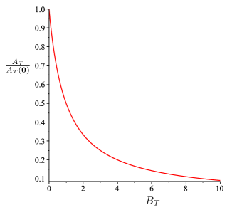
Figure 3: Normalised free antigen concentration, $A_{T}/A_{T}(\mathbf{0})$, as a function of the average of Ab concentrations $B_{T}(\mathbf{b})=M^{-1}\sum_{\mu=1}^{M}r_{\mu}b_{\mu}$.

For $P(\mathbf{0})>0$ we have to compute the function $\Phi$ in [57]. Since, $\Phi$ is a solution of a polynomial of degree $M_{A}+M_{S}$ [56], this could be non-nontrivial. But at least for $M_{A}+M_{S}=2$ we can compute this function analytically. Here $\Phi\left(\mathbf{B}^{T},\mathbf{B}^{S}\right)\equiv\Phi(B_{T},B_{S})$ is the solution of the quadratic equation

$$0 = \left(1+B_{S}\right)(1\!+\!B)y^{2}+\Big{\{}B_{T}\left(1\!+\!B_{S}\right)\left[P(\mathbf{0})\!-\!A_{T}(\mathbf{0})\right]+B_{S}(1\!+\!B_{T})\left[P(\mathbf{0})\!-\!A_{S}(\mathbf{0})\right]\Big{\}}y$$ (60)

$$\leavevmode\nobreak\ \leavevmode\nobreak\ \leavevmode\nobreak\ \leavevmode\nobreak\ \leavevmode\nobreak\ \leavevmode\nobreak\ \leavevmode\nobreak\ +\leavevmode\nobreak\ B_{S}B_{T}P(\mathbf{0})\left[P(\mathbf{0})\!-\!A_{S}(\mathbf{0})\!-\!A_{T}(\mathbf{0})\right].$$

Its determinant

$$D = \Big{(}B_{T}\left(1\!+\!B_{S}\right)\left[P(\mathbf{0})\!-\!A_{T}(\mathbf{0})\right]+B_{S}(1\!+\!B_{T})\left[P(\mathbf{0})\!-\!A_{S}(\mathbf{0})\right]\Big{)}^{2}$$

$$\leavevmode\nobreak\ \leavevmode\nobreak\ \leavevmode\nobreak\ \leavevmode\nobreak\ \leavevmode\nobreak\ \leavevmode\nobreak\ \leavevmode\nobreak\ \leavevmode\nobreak\ \leavevmode\nobreak\ \leavevmode\nobreak\ \leavevmode\nobreak\ \leavevmode\nobreak\ \leavevmode\nobreak\ \leavevmode\nobreak\ \leavevmode\nobreak\ \leavevmode\nobreak\ \leavevmode\nobreak\ \leavevmode\nobreak\ \leavevmode\nobreak\ \leavevmode\nobreak\ \leavevmode\nobreak\ \leavevmode\nobreak\ \leavevmode\nobreak\ \leavevmode\nobreak\ \leavevmode\nobreak\ \leavevmode\nobreak\ \leavevmode\nobreak\ \leavevmode\nobreak\ \leavevmode\nobreak\ -4B_{S}B_{T}\left(1\!+\!B_{S}\right)(1\!+\!B_{T})\,P(\mathbf{0})\left[P(\mathbf{0})\!-\!A_{S}(\mathbf{0})-A_{T}(\mathbf{0})\right]$$

is positive when $A_{T}(\mathbf{0})+A_{S}(\mathbf{0})\geq P(\mathbf{0})$, in which case the equation has two real solutions. Only one of them is positive:

$$\Phi(B,B_{S}) = \frac{B_{T}\left[A_{T}(\mathbf{0})\!-\!P(\mathbf{0})\right]}{2\left(1+B_{T}\right)}+\frac{B_{S}\left[A_{S}(\mathbf{0})\!-\!P(\mathbf{0})\right]}{2\left(1+B_{S}\right)}$$

$$+\leavevmode\nobreak\ \Bigg{\{}\left(\frac{B_{T}\left[A_{T}(\mathbf{0})\!-\!P(\mathbf{0})\right]}{2\left(1+B_{T}\right)}+\frac{B_{S}\left[A_{S}(\mathbf{0})\!-\!P(\mathbf{0})\right]}{2\left(1+B_{S}\right)}\right)^{2}+\frac{B_{T}B_{S}P(\mathbf{0})\left[A_{T}(\mathbf{0})\!+\!A_{S}(\mathbf{0})\!-\!P(\mathbf{0})\right]}{\left(1+B_{T}\right)\left(1+B_{S}\right)}\Bigg{\}}^{\frac{1}{2}}.$$

1.2 Bivalent Antibodies reacting with univalent target Antigen and self-Antigen

In this section we show that in the regime of ‘weak’ Abs, as considered in previous section, the amount of free Ag is not affected by the valency of Abs (22). To this end it is sufficient only to consider the case of bivalent Abs interacting with univalent target Ag and self-Ag. In particular we consider $M$ different bivalent Abs, represented by the symbols $\mathrm{Y}_{\mu}$ with $\mu\in\{1,\ldots,M\}$, forming complexes with univalent target Ag, $\triangle$, and univalent self-Ag, $\circ$. The formation of complexes is modelled by the following chemical reactions:

$$\circ+\mathrm{Y}_{\mu}\overset{{K_{\mu}^{S+}}}{\underset{{K_{\mu}^{S-}}}{\rightleftharpoons}}\overset{\circ}{\mathrm{Y}_{\mu}}\leavevmode\nobreak\ \leavevmode\nobreak\ \leavevmode\nobreak\ \leavevmode\nobreak\ \leavevmode\nobreak\ \leavevmode\nobreak\ \leavevmode\nobreak\ \leavevmode\nobreak\ \leavevmode\nobreak\ \leavevmode\nobreak\ \leavevmode\nobreak\ \circ+\overset{\circ}{\mathrm{Y}_{\mu}}\overset{{K_{\mu}^{S+}}}{\underset{{K_{\mu}^{S-}}}{\rightleftharpoons}}\overset{\!\!\!\!\circ\,\circ}{\mathrm{Y}_{\mu}}\leavevmode\nobreak\ \leavevmode\nobreak\ \leavevmode\nobreak\ \leavevmode\nobreak\ \leavevmode\nobreak\ \leavevmode\nobreak\ \leavevmode\nobreak\ \leavevmode\nobreak\ \leavevmode\nobreak\ \leavevmode\nobreak\ \leavevmode\nobreak\ \triangle+\mathrm{Y}_{\mu}\overset{{K_{\mu}^{N+}}}{\underset{{K_{\mu}^{N-}}}{\rightleftharpoons}}\overset{\triangle}{\mathrm{Y}_{\mu}}$$ (63)

$$\triangle+\overset{\triangle}{\mathrm{Y}_{\mu}}\overset{{K_{\mu}^{N+}}}{\underset{{K_{\mu}^{N-}}}{\rightleftharpoons}}\overset{\!\!\!\!\triangle\,\triangle}{\mathrm{Y}_{\mu}}\leavevmode\nobreak\ \leavevmode\nobreak\ \leavevmode\nobreak\ \leavevmode\nobreak\ \leavevmode\nobreak\ \leavevmode\nobreak\ \leavevmode\nobreak\ \leavevmode\nobreak\ \leavevmode\nobreak\ \circ+\overset{\triangle}{\mathrm{Y}_{\mu}}\overset{{K_{\mu}^{SN+}}}{\underset{{K_{\mu}^{SN-}}}{\rightleftharpoons}}\overset{\!\!\!\!\circ\,\triangle}{\mathrm{Y}_{\mu}}\leavevmode\nobreak\ \leavevmode\nobreak\ \leavevmode\nobreak\ \leavevmode\nobreak\ \leavevmode\nobreak\ \leavevmode\nobreak\ \leavevmode\nobreak\ \leavevmode\nobreak\ \triangle+\overset{\circ}{\mathrm{Y}_{\mu}}\overset{{K_{\mu}^{SN+}}}{\underset{{K_{\mu}^{SN-}}}{\rightleftharpoons}}\overset{\!\!\!\!\triangle\,\circ}{\mathrm{Y}_{\mu}}$$ (64)

In chemical equilibrium, the concentrations of free self-Ag, target Ag, and Ab, which will be denoted, respectively, by the symbols $\left[\circ\right]$, $\left[\triangle\right]$ and $\left[\mathrm{Y}_{\mu}\right]$, are related to the concentrations of bound species $\overset{\circ}{\mathrm{Y}_{\mu}}$, $\overset{\!\!\!\!\circ\,\circ}{\mathrm{Y}_{\mu}}$, $\overset{\triangle}{\mathrm{Y}_{\mu}}$, $\overset{\!\!\!\!\triangle\,\triangle}{\mathrm{Y}_{\mu}}$ and $\overset{\!\!\!\!\triangle\,\circ}{\mathrm{Y}_{\mu}}$, which we denote, respectively, by the symbols $[\overset{\circ}{\mathrm{Y}_{\mu}}]$, $[\overset{\!\!\!\!\circ\,\circ}{\mathrm{Y}_{\mu}}]$, $[\overset{\triangle}{\mathrm{Y}_{\mu}}]$, $[\overset{\!\!\!\!\triangle\,\triangle}{\mathrm{Y}_{\mu}}]$ and $[\overset{\!\!\!\!\triangle\,\circ}{\mathrm{Y}_{\mu}}]$, via the affinities $r_{\mu}^{S}={K_{\mu}^{S+}}\!/{K_{\mu}^{S-}}$, $r_{\mu}^{N}={K^{N+}_{\mu}}\!/{K^{N-}_{\mu}}$ and $r_{\mu}^{SN}={K_{\mu}^{SN+}}\!/{K_{\mu}^{SN-}}$ via

$$r_{\mu}^{S}=\frac{[\overset{\circ}{\mathrm{Y}_{\mu}}]}{\left[\circ\right]\left[\mathrm{Y}_{\mu}\right]}=\frac{[\overset{\!\!\!\!\circ\,\circ}{\mathrm{Y}_{\mu}}]}{\left[\circ\right][\overset{\circ}{\mathrm{Y}_{\mu}}]}\leavevmode\nobreak\ \leavevmode\nobreak\ \leavevmode\nobreak\ \leavevmode\nobreak\ \leavevmode\nobreak\ \leavevmode\nobreak\ \leavevmode\nobreak\ \leavevmode\nobreak\ r_{\mu}^{N}=\frac{[\overset{\triangle}{\mathrm{Y}_{\mu}}]}{\left[\triangle\right]\left[\mathrm{Y}_{\mu}\right]}=\frac{[\overset{\!\!\!\!\triangle\,\triangle}{\mathrm{Y}_{\mu}}]}{\left[\triangle\right][\overset{\triangle}{\mathrm{Y}_{\mu}}]}\leavevmode\nobreak\ \leavevmode\nobreak\ \leavevmode\nobreak\ \leavevmode\nobreak\ \leavevmode\nobreak\ \leavevmode\nobreak\ \leavevmode\nobreak\ \leavevmode\nobreak\ r_{\mu}^{SN}=\frac{[\overset{\!\!\!\!\triangle\,\circ}{\mathrm{Y}_{\mu}}]}{[\triangle][\overset{\circ}{\mathrm{Y}_{\mu}}]}=\frac{[\overset{\!\!\!\!\circ\,\triangle}{\mathrm{Y}_{\mu}}]}{[\circ][\overset{\triangle}{\mathrm{Y}_{\mu}}]}.$$ (65)

If the initial concentrations of species $\circ$, $\triangle$ and $\mathrm{Y}_{\mu}$ are, respectively, given by $\left[\circ\right]_{0}$, $\left[\triangle\right]_{0}$ and $\left[\mathrm{Y}_{\mu}\right]_{0}$ then, because of the mass conservation, we have

$$\left[\circ\right]_{0} = \left[\circ\right]+\sum_{\mu=1}^{M}\,[\overset{\circ}{\mathrm{Y}_{\mu}}]+\sum_{\mu=1}^{M}\,[\overset{\!\!\!\!\circ\,\triangle}{\mathrm{Y}_{\mu}}]+\sum_{\mu=1}^{M}\,[\overset{\!\!\!\!\triangle\,\circ}{\mathrm{Y}_{\mu}}]+2\sum_{\mu=1}^{M}\,[\overset{\!\!\!\!\circ\,\circ}{\mathrm{Y}_{\mu}}]$$ (66)

$$\left[\triangle\right]_{0} = \left[\triangle\right]+\sum_{\mu=1}^{M}\,[\overset{\triangle}{\mathrm{Y}_{\mu}}]+\sum_{\mu=1}^{M}\,[\overset{\!\!\!\!\circ\,\triangle}{\mathrm{Y}_{\mu}}]+\sum_{\mu=1}^{M}\,[\overset{\!\!\!\!\triangle\,\circ}{\mathrm{Y}_{\mu}}]+2\sum_{\mu=1}^{M}\,[\,\overset{\!\!\!\!\triangle\,\triangle}{\mathrm{Y}_{\mu}}]$$

$$\left[\mathrm{Y}_{\mu}\right]_{0} = \left[\mathrm{Y}_{\mu}\right]+[\overset{\circ}{\mathrm{Y}_{\mu}}]+[\overset{\triangle}{\mathrm{Y}_{\mu}}]+[\overset{\!\!\!\!\circ\,\triangle}{\mathrm{Y}_{\mu}}]+[\overset{\!\!\!\!\triangle\,\circ}{\mathrm{Y}_{\mu}}]+[\overset{\!\!\!\!\circ\,\circ}{\mathrm{Y}_{\mu}}]+[\,\overset{\!\!\!\!\triangle\,\triangle}{\mathrm{Y}_{\mu}}].$$

Using the equilibrium relations [65] in the above three lines now gives us

$$\left[\circ\right] = \frac{\left[\circ\right]_{0}}{1+\sum_{\mu=1}^{M}\left[r_{\mu}^{S}+r_{\mu}^{SN}\left[\triangle\right]\left(r_{\mu}^{S}+r_{\mu}^{N}\right)+2{r_{\mu}^{S}}^{2}\left[\circ\right]\right]\left[\mathrm{Y}_{\mu}\right]}$$ (67)

$$\left[\triangle\right] = \frac{\left[\triangle\right]_{0}}{1+\sum_{\mu=1}^{M}\left[r_{\mu}^{N}+r_{\mu}^{SN}\left[\circ\right]\left(r_{\mu}^{S}+r_{\mu}^{N}\right)+2{r_{\mu}^{N}}^{2}\left[\triangle\right]\right]\left[\mathrm{Y}_{\mu}\right]},$$

where

$$\left[\mathrm{Y}_{\mu}\right] = \frac{\left[\mathrm{Y}_{\mu}\right]_{0}}{1+r_{\mu}^{S}\left[\circ\right]+r_{\mu}^{N}\left[\triangle\right]+r_{\mu}^{SN}\left[\circ\right]\left[\triangle\right]\left\{r_{\mu}^{S}+r_{\mu}^{N}\right\}+{r_{\mu}^{S}}^{2}\left[\circ\right]^{2}+{r_{\mu}^{N}}^{2}\left[\triangle\right]^{2}}.$$ (68)

Finally, with the notation $A_{S}=\left[\circ\right]$, $A_{S}(\mathbf{0})=\left[\circ\right]_{0}$, $A_{T}=\left[\triangle\right]$, $A_{T}(\mathbf{0})=\left[\triangle\right]_{0}$ and $b_{\mu}=\left[\mathrm{Y}_{\mu}\right]_{0}$, we obtain the recursive equations

$$A_{S} = \frac{A_{S}(\mathbf{0})}{1+\sum_{\mu=1}^{M}\frac{\left[r_{\mu}^{S}+r_{\mu}^{SN}\left(r_{\mu}^{S}+r_{\mu}^{N}\right)A_{T}+2{r_{\mu}^{S}}^{2}A_{S}\right]\,b_{\mu}}{1+r_{\mu}^{S}A_{S}+r_{\mu}^{N}A_{T}+r_{\mu}^{SN}\left\{r_{\mu}^{S}+r_{\mu}^{N}\right\}A_{S}A_{T}+{r_{\mu}^{S}}^{2}A_{S}^{2}+{r_{\mu}^{N}}^{2}A_{T}^{2}}}$$ (69)

$$A_{T} = \frac{A_{T}(\mathbf{0})}{1+\sum_{\mu=1}^{M}\frac{\left[r_{\mu}^{N}+r_{\mu}^{SN}\left(r_{\mu}^{S}+r_{\mu}^{N}\right)A_{S}+2{r_{\mu}^{N}}^{2}A_{T}\right]\,b_{\mu}}{1+r_{\mu}^{S}A_{S}+r_{\mu}^{N}A_{T}+r_{\mu}^{SN}\left\{r_{\mu}^{S}+r_{\mu}^{N}\right\}A_{S}A_{T}+{r_{\mu}^{S}}^{2}A_{S}^{2}+{r_{\mu}^{N}}^{2}A_{T}^{2}}}.$$

Now let us redefine $r_{\mu}=r_{\mu}/M$, $r_{\mu}^{S}=r_{\mu}^{S}/M$ and $r_{\mu}^{SN}=r_{\mu}^{SN}/M$, and consider the relevant term in our expression for $A_{S}$:

$$\frac{\left[r_{\mu}^{S}+r_{\mu}^{SN}\left(r_{\mu}^{S}+r_{\mu}^{N}\right)A_{T}+2{r_{\mu}^{S}}^{2}A_{S}\right]b_{\mu}}{1+r_{\mu}^{S}A_{S}+r_{\mu}^{N}A_{T}+r_{\mu}^{SN}\left\{r_{\mu}^{S}+r_{\mu}^{N}\right\}A_{S}A_{T}+{r_{\mu}^{S}}^{2}A_{S}^{2}+{r_{\mu}^{N}}^{2}A_{T}^{2}}$$

$$= \frac{\frac{r_{\mu}^{S}}{M}b_{\mu}+\left[r_{\mu}^{SN}\left(r_{\mu}^{S}+r_{\mu}^{N}\right)A_{T}+2{r_{\mu}^{S}}^{2}A_{S}\right]\frac{b_{\mu}}{M^{2}}}{1+\left[r_{\mu}^{S}A_{S}+r_{\mu}^{N}A_{T}\right]\frac{1}{M}+\left[r_{\mu}^{SN}\left\{r_{\mu}^{S}+r_{\mu}^{N}\right\}A_{S}A_{T}+{r_{\mu}^{S}}^{2}A^{2}_{S}+{r_{\mu}^{N}}^{2}A_{T}^{2}\right]\frac{1}{M^{2}}}$$

$$= \frac{r_{\mu}^{S}\,b_{\mu}}{M}+O\left(\phi^{2}(M)/M^{2}\right)$$

Here we assumed that $A_{S},A\propto\phi(M)$, where $\phi(M)=o(M)$. The same argument applies to the corresponding term in the equation for $A_{T}$, giving us $r_{\mu}b_{\mu}/M+O\left(\phi^{2}(M)/M^{2}\right)$ and hence

$$A_{S}(\mathbf{b})=\frac{A_{S}(\mathbf{0})}{1+\frac{1}{M}\sum_{\mu=1}^{M}r_{\mu}^{S}b_{\mu}}\leavevmode\nobreak\ \leavevmode\nobreak\ \leavevmode\nobreak\ \leavevmode\nobreak\ \leavevmode\nobreak\ \leavevmode\nobreak\ \leavevmode\nobreak\ \leavevmode\nobreak\ A_{T}(\mathbf{b})=\frac{A_{T}(\mathbf{0})}{1+\frac{1}{M}\sum_{\mu=1}^{M}r_{\mu}^{N}b_{\mu}}$$ (71)

for $M\rightarrow\infty$, so we recover the result [59] for univalent Abs interacting with two types of Ag. The above argument easily generalises to include multiple univalent Ags and binding of Ag-Ab complexes.

2 Analysis of Antibody Dynamics

In this section we study the Euler-Lagrange equation

$$\Lambda_{\mu}\frac{\mathrm{d}^{2}}{\mathrm{d}t^{2}}{b}_{\mu} = -\frac{\partial}{\partial b_{\mu}}\left[A_{T}(\mathbf{b})-\gamma A_{S}(\mathbf{b})\right],$$ (72)

where $\Lambda_{\mu}\geq 0$ and $\gamma\geq 0$, with the ‘energy’ functions $A_{T}(\mathbf{b})$ and $A_{S}(\mathbf{b})$ derived in section 1.1.

2.1 Binding of univalent Antigens by univalent Antibodies in the presence of univalent self-Antigens

Let us define the total potential ‘energy’

$$A_{\gamma}\left(\mathbf{B}^{T},\mathbf{B}^{S}\right) = A_{T}\left(\mathbf{B}^{T},\mathbf{B}^{S}\right)-\gamma A_{S}\left(\mathbf{B}^{T},\mathbf{B}^{S}\right),$$ (73)

where $A_{T}\left(\mathbf{B}^{T},\mathbf{B}^{S}\right)\equiv A_{T}(\mathbf{b})$ and $A_{S}\left(\mathbf{B}^{T},\mathbf{B}^{S}\right)\equiv A_{S}(\mathbf{b})$, with $A_{T}(\mathbf{b})$ and $A_{S}(\mathbf{b})$ as defined in [58], and we consider equation [72] for this energy function:

$$\Lambda_{\mu}\frac{\mathrm{d}^{2}}{\mathrm{d}t^{2}}{b}_{\mu} = -\frac{\partial}{\partial b_{\mu}}A_{\gamma}\left(\mathbf{B}^{T},\mathbf{B}^{S}\right)\leavevmode\nobreak\ =\leavevmode\nobreak\ -\sum_{k=1}^{M_{A}}\frac{\partial A_{\gamma}}{\partial B^{T}_{k}}\frac{\partial B^{T}_{k}}{\partial b_{\mu}}-\sum_{\ell=1}^{M_{S}}\frac{\partial A_{\gamma}}{\partial B^{S}_{\ell}}\frac{\partial B^{S}_{\ell}}{\partial b_{\mu}}$$

$$= -\sum_{k=1}^{M_{A}}\frac{\partial A_{\gamma}}{\partial B^{T}_{k}}\frac{r_{\mu k}}{M}-\sum_{\ell=1}^{M_{S}}\frac{\partial A_{\gamma}}{\partial B^{S}_{\ell}}\frac{r^{S}_{\mu\ell}}{M}$$

Assuming that $\Lambda_{\mu}=\lambda_{\mu}\phi(M)/M$, where $\phi(M)=o(M)$, and using definition [1.1] above, allows us to derive the following equations for the set of macroscopic observables $\mathbf{B}^{T}$ and $\mathbf{B}^{S}$:

$$\frac{\mathrm{d}^{2}}{\mathrm{d}t^{2}}{B}_{v}^{T} = -\sum_{k=1}^{M_{A}}(\mathbf{r}_{v}\!\cdot\mathbf{r}_{k})\frac{\partial}{\partial B_{k}^{T}}A_{\gamma}\left(\mathbf{B}^{T}\!,\mathbf{B}^{S}\right)-\sum_{\ell=1}^{M_{S}}(\mathbf{r}_{v}\!\cdot\mathbf{r}_{\ell}^{S})\frac{\partial}{\partial B^{S}_{\ell}}A_{\gamma}\left(\mathbf{B}^{T}\!,\mathbf{B}^{S}\right)$$ (74)

$$\frac{\mathrm{d}^{2}}{\mathrm{d}t^{2}}{B}_{u}^{S} = -\sum_{k=1}^{M_{A}}(\mathbf{r}_{u}^{S}\!\cdot\mathbf{r}_{k})\frac{\partial}{\partial B_{k}^{T}}A_{\gamma}\left(\mathbf{B}^{T}\!,\mathbf{B}^{S}\right)-\sum_{\ell=1}^{M_{S}}(\mathbf{r}_{u}^{S}\!\cdot\mathbf{r}^{S}_{\ell})\frac{\partial}{\partial B^{S}_{\ell}}A_{\gamma}\left(\mathbf{B}^{T}\!,\mathbf{B}^{S}\right)$$ (75)

with the short-hand $\mathbf{x}\cdot\mathbf{y}=M^{-1}\sum_{\mu=1}^{M}\lambda_{\mu}^{-1}x_{\mu}y_{\mu}$, with associated inner product norm $|\mathbf{x}|=\sqrt{\mathbf{x}\cdot\mathbf{x}}$.

In the special simplified case where each Ab $\mu$ interacts with only one type of Ag, we will have $\mathbf{r}_{v}\cdot\mathbf{r}_{k}=0$ if $v\neq k$, $\mathbf{r}_{v}\cdot\mathbf{r}_{\ell}^{S}=0$, etc., and the system of equations [74] simplifies to

$$\frac{1}{|\mathbf{r}_{v}|^{2}}\frac{\mathrm{d}^{2}}{\mathrm{d}t^{2}}{B}_{v}=-\frac{\partial}{\partial B_{v}}A_{\gamma}\!\left(\mathbf{B},\mathbf{B}^{S}\right)\leavevmode\nobreak\ \leavevmode\nobreak\ \leavevmode\nobreak\ \leavevmode\nobreak\ \leavevmode\nobreak\ \leavevmode\nobreak\ \leavevmode\nobreak\ \leavevmode\nobreak\ \frac{1}{|\mathbf{r}_{u}^{S}|^{2}}\frac{\mathrm{d}^{2}}{\mathrm{d}t^{2}}{B}_{u}^{S}=-\frac{\partial}{\partial B^{S}_{u}}A_{\gamma}\!\left(\mathbf{B},\mathbf{B}^{S}\right).$$

We note that the above simplified macroscopic dynamics is conservative (23), with the energy function

$$E\!\left(\mathbf{B}^{T}\!,\frac{\mathrm{d}}{\mathrm{d}t}{\mathbf{B}^{T}};\mathbf{B}^{S}\!,\frac{\mathrm{d}}{\mathrm{d}t}{\mathbf{B}}^{S}\right) = \sum_{v=1}^{M_{A}}\frac{1}{2|\mathbf{r}_{v}|^{2}}\Big{(}\frac{\mathrm{d}B^{T}_{v}}{\mathrm{d}t}\Big{)}^{\!2}+\sum_{u=1}^{M_{S}}\frac{1}{2|\mathbf{r}_{u}^{S}|^{2}}\Big{(}\frac{\mathrm{d}B^{S}_{u}}{\mathrm{d}t}\Big{)}^{\!2}+A_{\gamma}\!\left(\mathbf{B}^{T},\mathbf{B}^{S}\right)$$ (76)

where the first two terms play the role of ‘kinetic’ energies, and the third term is the ‘potential’ energy. The factors $1/|\mathbf{r}_{v}|^{2}$ and $1/|\mathbf{r}_{u}^{S}|^{2}$ can be seen as ‘masses’. So [2.1] describes the motion (23) of $M_{A}+M_{S}$ ‘particles’, with distinct masses, in a potential field with potential energy [73].

Let us now assume that the numbers of target and self Ags are equal, i.e. $M_{A}=M_{S}$, and that each Ab $\mu$ simultaneously interacts with two types of Ag, one target and one self (see Figure 4 for $M_{A}=M_{S}=1$). Then the affinity vectors $\mathbf{r}_{v}$ and $\mathbf{r}_{u}^{S}$ satisfy the orthogonality conditions $\mathbf{r}_{v}\cdot\mathbf{r}_{k}=0$ if $k\neq v$ and $\mathbf{r}_{u}^{S}\cdot\mathbf{r}_{\ell}^{S}=0$ if $\ell\neq u$, i.e. each row in the affinity matrices $\mathbf{R}^{T}=(\mathbf{r}_{1},\ldots,\mathbf{r}_{M_{A}})$ and $\mathbf{R}^{S}=(\mathbf{r}^{S}_{1},\ldots,\mathbf{r}^{S}_{M_{A}})$ has exactly one positive component. Also $\mathbf{r}_{v}\cdot\mathbf{r}_{\ell}^{S}=0$ if $\ell\neq u$, so, up to a permutation of columns, the matrices $\mathbf{R}^{T}$ and $\mathbf{R}^{S}$ are the same. Our equations then simplify to

$$\frac{\mathrm{d}^{2}}{\mathrm{d}t^{2}}{B}_{v}^{T} = -\frac{\partial}{\partial B_{v}^{T}}A_{\gamma}\!\left(\mathbf{B}^{T}\!,\mathbf{B}^{S}\right)|\mathbf{r}_{v}|^{2}-\frac{\partial}{\partial B^{S}_{u}}A_{\gamma}\left(\mathbf{B}^{T}\!,\mathbf{B}^{S}\right)(\mathbf{r}_{v}\!\cdot\mathbf{r}_{u}^{S})$$ (77)

$$\frac{\mathrm{d}^{2}}{\mathrm{d}t^{2}}{B}_{u}^{S} = -\frac{\partial}{\partial B_{v}^{T}}A_{\gamma}\left(\mathbf{B}^{T}\!,\mathbf{B}^{S}\right)(\mathbf{r}_{u}^{S}\!\cdot\mathbf{r}_{v})-\frac{\partial}{\partial B^{S}_{u}}A_{\gamma}\left(\mathbf{B}^{T}\!,\mathbf{B}^{S}\right)|\mathbf{r}_{u}^{S}|^{2}.$$ (78)

Figure 4: Network representation of $M$ different populations of univalent Abs (small blue circles) interacting with populations of univalent target Ag (red triangle) and self-Ag (large blue circle). Ab $\mu$ is interacting with the target Ag and self-Ag with, strengths (affinities) $r_{\mu}$ and $r_{\mu}^{S}$, respectively. The Ags are interacting with all Abs.

Assuming that the above system is in ‘mechanical’ equilibrium, $\mathrm{d}^{2}{B}^{T}_{v}/\mathrm{d}t^{2}=\mathrm{d}^{2}{B}_{u}^{S}/\mathrm{d}t^{2}=0$, leads us to the two equalities

$$-\frac{\partial A_{\gamma}\!\left(\mathbf{B}^{T}\!,\mathbf{B}^{S}\right)/\partial B^{T}_{v}}{\partial A_{\gamma}\left(\mathbf{B}^{T}\!,\mathbf{B}^{S}\right)/\partial B^{S}_{u}}=\frac{(\mathbf{r}_{v}\cdot\mathbf{r}_{u}^{S})}{|\mathbf{r}_{v}|^{2}}\leavevmode\nobreak\ \leavevmode\nobreak\ \leavevmode\nobreak\ \leavevmode\nobreak\ \leavevmode\nobreak\ \leavevmode\nobreak\ \leavevmode\nobreak\ \leavevmode\nobreak\ -\frac{\partial A_{\gamma}\!\left(\mathbf{B}^{T}\!,\mathbf{B}^{S}\right)/\partial B^{T}_{v}}{\partial A_{\gamma}\left(\mathbf{B}^{T}\!,\mathbf{B}^{S}\right)/\partial B^{S}_{u}}=\frac{|\mathbf{r}_{u}^{S}|^{2}}{(\mathbf{r}_{u}^{S}\cdot\mathbf{r}_{v})}$$ (79)

and hence

$$(\mathbf{r}_{v}\cdot\mathbf{r}_{u}^{S})^{2} = |\mathbf{r}_{u}^{S}|^{2}|\mathbf{r}_{v}|^{2}.$$ (80)

We note that this will be true if and only if $\mathbf{r}=\alpha(v,u)\mathbf{r}_{u}^{S}$, for some $\alpha(v,u)>0$. Using this in [77] gives us the equations

$$\frac{\mathrm{d}^{2}}{\mathrm{d}t^{2}}{B}_{v} = -\frac{\partial}{\partial B_{v}}A_{\gamma}\!\left(\mathbf{B},\mathbf{B}^{S}\right)\alpha^{2}(v,u)|\mathbf{r}_{u}^{S}|^{2}-\frac{\partial}{\partial B^{S}_{u}}A_{\gamma}\left(\mathbf{B},\mathbf{B}^{S}\right)\alpha(v,u)|\mathbf{r}_{u}^{S}|^{2}$$ (81)

$$\frac{\mathrm{d}^{2}}{\mathrm{d}t^{2}}{B}_{u}^{S} = -\frac{\partial}{\partial B_{v}}A_{\gamma}\left(\mathbf{B},\mathbf{B}^{S}\right)\alpha(v,u)|\mathbf{r}_{u}^{S}|^{2}-\frac{\partial}{\partial B^{S}_{u}}A_{\gamma}\left(\mathbf{B},\mathbf{B}^{S}\right)|\mathbf{r}_{u}^{S}|^{2}$$

We note that $\alpha(v,u)$ generates a mapping $\mathbf{r}_{v}=\alpha(v,u)\,\mathbf{r}_{u}^{S}$ between the affinities $\mathbf{r}_{v}$ and $\mathbf{r}_{u}^{S}$. Without loss of generality, we can always re-label the antibodies such that $u=v$, so that we only need $\alpha(v,v)\equiv\alpha(v)$. Equation [81] can then be simplified to

$$\frac{1}{\alpha(v)|\mathbf{r}_{v}^{S}|^{2}}\frac{\mathrm{d}^{2}}{\mathrm{d}t^{2}}{B}^{T}_{v} = -\frac{\partial}{\partial B^{T}_{v}}A_{\gamma}\!\left(\mathbf{B}^{T}\!,\mathbf{B}^{S}\right)\alpha(v)-\frac{\partial}{\partial B^{S}_{v}}A_{\gamma}\left(\mathbf{B}^{T}\!,\mathbf{B}^{S}\right)$$ (82)

$$\frac{1}{|\mathbf{r}_{v}^{S}|^{2}}\frac{\mathrm{d}^{2}}{\mathrm{d}t^{2}}{B}_{v}^{S} = -\frac{\partial}{\partial B^{T}_{v}}A_{\gamma}\left(\mathbf{B}^{T}\!,\mathbf{B}^{S}\right)\alpha(v)-\frac{\partial}{\partial B^{S}_{v}}A_{\gamma}\left(\mathbf{B}^{T}\!,\mathbf{B}^{S}\right).$$

Furthermore, since now $B^{T}_{v}=\alpha(v)B^{S}_{v}$ the above reduces to the single equation

$$\frac{1}{|\mathbf{r}_{v}^{S}|^{2}}\frac{\mathrm{d}^{2}}{\mathrm{d}t^{2}}{B}_{v}^{S} = -\alpha(v)\frac{\partial}{\partial B^{T}_{v}}A_{\gamma}\left(\mathbf{B}^{T},\mathbf{B}^{S}\right)-\frac{\partial}{\partial B^{S}_{v}}A_{\gamma}\left(\mathbf{B}^{T},\mathbf{B}^{S}\right),$$ (83)

where the partial derivatives are evaluated at $B^{T}_{v}=\alpha(v)B^{S}_{v}$.

The macroscopic dynamics [83] is conservative when $P(\mathbf{0})=0$. In this case the potential energy [73] is given by

$$A_{\gamma}\left(\mathbf{B}^{T}\!,\mathbf{B}^{S}\right) = \sum_{v=1}^{M_{A}}\frac{A^{T}_{v}(\mathbf{0})}{1+B^{T}_{v}}-\gamma\sum_{u=1}^{M_{S}}\frac{A^{S}_{u}(\mathbf{0})}{1+B^{S}_{u}}$$ (84)

and equation [83] reduces to

$$\frac{1}{|\mathbf{r}_{v}^{S}|^{2}}\frac{\mathrm{d}^{2}}{\mathrm{d}t^{2}}{B}_{v}^{S} = -\frac{\partial}{\partial B^{S}_{v}}\left\{\frac{A_{v}^{0T}}{1+\alpha(v)B^{S}_{v}}-\gamma\frac{A^{0S}_{v}}{1+B^{S}_{v}}\right\},$$ (85)

so this dynamics is conservative, with the energy

$$E_{v}\!\left(B^{S}_{v},\frac{\mathrm{d}}{\mathrm{d}t}{B}_{v}^{S}\right) = \frac{1}{2|\mathbf{r}_{v}^{S}|^{2}}\Big{(}\frac{\mathrm{d}}{\mathrm{d}t}{B}_{v}^{S}\Big{)}^{2}+\frac{A_{v}^{0T}}{\left(1+\alpha(v)B^{S}_{v}\right)}-\gamma\frac{A^{0S}_{v}}{\left(1+B^{S}_{v}\right)},$$ (86)

describing the ‘motion’ a ‘particle’ of ‘mass’ $1/|\mathbf{r}_{v}^{S}|^{2}$ in a potential field. If at time $t=0$ we are given the initial position $B^{S}_{v}(0)$ and velocity $(\mathrm{d}{B}^{S}_{v}/\mathrm{d}t)(0)$ of this particle, then for all $t>0$ we have due to energy conservation:

$$E_{v}\!\left(B^{S}_{v},\frac{\mathrm{d}}{\mathrm{d}t}{B}_{v}^{S}\right) = E_{v}\!\left(B^{S}_{v}(0),(\frac{\mathrm{d}}{\mathrm{d}t}{B}_{v}^{S})(0)\right).$$ (87)

2.2 Binding of univalent Antigen by univalent Antibodies in the presence of univalent self-Antigen

The dynamics [72] with the energy function [84] can be solved in a full detail when $M_{A}=M_{S}=1$ (see Figure 4). Here the Euler-Lagrange equation is

$$\Lambda_{\mu}\frac{\mathrm{d}^{2}}{\mathrm{d}t^{2}}{b}_{\mu} = -\frac{\partial}{\partial b_{\mu}}\left[\frac{A_{T}(\mathbf{0})}{1+B_{T}(\mathbf{b})}-\gamma\frac{A_{S}(\mathbf{0})}{1+B_{S}(\mathbf{b})}\right]$$

$$= \frac{A_{T}(\mathbf{0})}{\left(1+B_{T}(\mathbf{b})\right)^{2}}\frac{r_{\mu}}{M}-\gamma\frac{A_{S}(\mathbf{0})\,}{\left(1+B_{S}(\mathbf{b})\right)^{2}}\frac{r^{S}_{\mu}}{M},$$

where $B_{T}(\mathbf{b})=M^{-1}\sum_{\nu=1}^{M}r_{\nu}\,b_{\nu}(t)$ and $B_{S}(\mathbf{b})=M^{-1}\sum_{\nu=1}^{M}r^{S}_{\nu}\,b_{\nu}$. The latter two macroscopic observables are governed by the equations

$$\frac{\mathrm{d}^{2}}{\mathrm{d}t^{2}}{B}=\frac{A_{T}^{0}|\mathbf{r}|^{2}}{\left(1+B_{T}\right)^{2}}-\gamma\frac{A_{S}^{0}(\mathbf{r}\cdot\mathbf{r}^{S})}{\left(1+B_{S}\right)^{2}}\leavevmode\nobreak\ \leavevmode\nobreak\ \leavevmode\nobreak\ \leavevmode\nobreak\ \leavevmode\nobreak\ \leavevmode\nobreak\ \leavevmode\nobreak\ \leavevmode\nobreak\ \leavevmode\nobreak\ \leavevmode\nobreak\ \leavevmode\nobreak\ \frac{\mathrm{d}^{2}}{\mathrm{d}t^{2}}{B}_{S}=\frac{A_{T}^{0}(\mathbf{r}\cdot\mathbf{r}^{S})}{\left(1+B_{T}\right)^{2}}-\gamma\frac{A_{S}^{0}|\mathbf{r}^{S}|^{2}}{\left(1+B_{S}\right)^{2}},$$ (89)

where $B_{T}\equiv B(\mathbf{b})$ and $B_{S}\equiv B_{S}(\mathbf{b})$, with initial conditions $\{(\mathrm{d}{B_{T}}/\mathrm{d}t)(0),(\mathrm{d}{B}_{S}/\mathrm{d}t)(0),B_{T}(0),B_{S}(0)\}$. So the above equations are a special case of [74,75]. Furthermore, the average concentration of Abs $\tilde{B}(\mathbf{b})=M^{-1}\sum_{\nu=1}^{M}b_{\nu}$ is governed by

$$\frac{\mathrm{d}^{2}}{\mathrm{d}t^{2}}{\tilde{B}} = \frac{A_{T}^{0}(\mathbf{r}\cdot\mathbf{1})}{\left(1+B_{T}\right)^{2}}-\gamma\frac{A_{S}^{0}(\mathbf{r}^{S}\!\cdot\mathbf{1})}{\left(1+B_{S}\right)^{2}}.$$ (90)

The simplest case is that where each Ab is either self-reactive or non-self-reactive (never both), i.e. for all $\mu$ either $r_{\mu}=0$ and $r^{S}_{\mu}>0$ or $r_{\mu}>0$ and $r^{S}_{\mu}=0$. This implies that $(\mathbf{r}\cdot\mathbf{r}^{S})=0$ in [89], giving us the two independent equations

$$\frac{\mathrm{d}^{2}}{\mathrm{d}t^{2}}{B}_{T}=\frac{A_{T}^{0}|\mathbf{r}|^{2}}{\left(1+B_{T}\right)^{2}}\leavevmode\nobreak\ \leavevmode\nobreak\ \leavevmode\nobreak\ \leavevmode\nobreak\ \leavevmode\nobreak\ \leavevmode\nobreak\ \leavevmode\nobreak\ \leavevmode\nobreak\ \leavevmode\nobreak\ \leavevmode\nobreak\ \frac{\mathrm{d}^{2}}{\mathrm{d}t^{2}}{B}_{S}=-\gamma\frac{A_{S}^{0}|\mathbf{r}^{S}|^{2}}{\left(1+B_{S}\right)^{2}}.$$ (91)

We note that above is a special case of [2.1], so the dynamics of $B_{T}$ is conservative with the energy

$$E\!\left(B_{T},\frac{\mathrm{d}}{\mathrm{d}t}{B_{T}}\right) = \frac{1}{2|\mathbf{r}|^{2}}\Big{(}\frac{\mathrm{d}}{\mathrm{d}t}{B_{T}}\Big{)}^{2}+\frac{A_{T}^{0}}{1+B_{T}},$$ (92)

Since energy is conserved, one can then use the identity $E\!\left(B_{T},\mathrm{d}{B_{T}}/\mathrm{d}t\right)=E\left(B_{T}(0),(\mathrm{d}{B_{T}}/\mathrm{d}t)(0)\right)$ to obtain a simple equation for $\mathrm{d}{B}/\mathrm{d}t$. For the initial conditions $(\mathrm{d}{B_{T}}/\mathrm{d}t)(0)=B_{T}(0)=0$ this equation is given by

$$\frac{\mathrm{d}}{\mathrm{d}t}{B_{T}} = \sqrt{2A_{T}^{0}|\mathbf{r}|^{2}\frac{B_{T}}{1+B_{T}}}.$$ (93)

The function $\sqrt{B/(1\!+\!B)}\in[0,1]$ is monotonic increasing and concave for $B\in[\,0,\infty)$. Hence $B_{T}(t)$ is bounded from above by $\sqrt{2A^{0}|\mathbf{r}|^{2}}\,t$, saturating this upper bound as $t\rightarrow\infty$. Furthermore, the (normalised) amount of antigen $A_{T}/A(\mathbf{0})=1/(1\!+\!B_{T}(t))$ is bounded from below by $1/(1\!+\!\sqrt{2A^{0}|\mathbf{r}|^{2})\,t}$. Also the dynamics of $B_{S}$ in [91] is conservative, with energy

$$E\!\left(B_{S},\frac{\mathrm{d}}{\mathrm{d}t}{B}_{S}\right) = \frac{1}{2|\mathbf{r}^{S}|^{2}}\Big{(}\frac{\mathrm{d}}{\mathrm{d}t}{B}_{S}\Big{)}^{2}-\frac{\gamma A^{0}_{S}}{1+B_{S}},$$ (94)

and using $E\!\left(B_{S},\mathrm{d}{B}_{S}/\mathrm{d}t\right)=E\!\left(B_{S}(0),(\mathrm{d}{B}_{S}/\mathrm{d}t)(0)\right)$, with initial conditions $(\mathrm{d}{B}_{S}/\mathrm{d}t)(0)=B_{S}(0)=0$, gives us the equation

$$\Big{(}\frac{\mathrm{d}}{\mathrm{d}t}{B}_{S}\Big{)}^{2} = -2\gamma A_{S}^{0}|\mathbf{r}^{S}|^{2}\frac{B_{S}}{1+B_{S}}$$ (95)

which for $\gamma>0$ has only the trivial solution $B_{S}=0$. Values $\gamma<0$ lead to self-antigen removal and hence are not desirable.

Further results for [89] can in equilibrium states, defined by $\mathrm{d}^{2}{B_{T}}/\mathrm{d}t^{2}=\mathrm{d}^{2}{B_{S}}/\mathrm{d}t^{2}=0$. From these conditions we infer that $(\mathbf{r}\cdot\mathbf{r}^{S})^{2}=\mathbf{r}^{2}(\mathbf{r}^{S})^{2}$, hence $r_{\mu}=\alpha\,r^{S}_{\mu}$ for some $\alpha>0$. This, in return, via the definitions of $B_{T}$ and $B_{S}$, implies $B_{T}=\alpha B_{S}$ and hence the system [89] reduces to a single equation:

$$\frac{\mathrm{d}^{2}}{\mathrm{d}t^{2}}{B}_{S} = A_{S}^{0}|\mathbf{r}^{S}|^{2}\left[\frac{\alpha\beta}{\left(1+\alpha B_{S}\right)^{2}}-\frac{\gamma}{\left(1+B_{S}\right)^{2}}\right],$$ (96)

where we defined $\beta=A_{T}^{0}/A_{S}^{0}$. Furthermore, for equation [90], governing the average concentration of antibodies $\tilde{B}$, we obtain

$$\frac{\mathrm{d}^{2}}{\mathrm{d}t^{2}}{\tilde{B}} = A_{S}^{0}(\mathbf{r}^{S}\!\cdot\mathbf{1})\!\left[\frac{\alpha\beta}{\left(1+\alpha B_{S}\right)^{2}}-\frac{\gamma}{\left(1+B_{S}\right)^{2}}\right].$$ (97)

Thus the two equations [96] and [97] are related according to $|\mathbf{r}^{S}|^{2}\mathrm{d}^{2}\tilde{B}/\mathrm{d}t^{2}=(\mathbf{r}^{S}\!\cdot\mathbf{1})\mathrm{d}^{2}{B}_{S}/\mathrm{d}t^{2}$, and hence

$$\tilde{B} = [(\mathbf{r}^{S}\!\cdot\mathbf{1})/|\mathbf{r}^{S}|^{2}]B_{S}.$$ (98)

The dynamics [96] conserves the energy

$$E\left(B_{S},\frac{\mathrm{d}}{\mathrm{d}t}{B}_{S}\right) = \frac{1}{2|\mathbf{r}^{S}|^{2}}\Big{(}\frac{\mathrm{d}}{\mathrm{d}t}{B}_{S}\Big{)}^{2}+A_{S}^{0}\left[\frac{\beta}{\left(1+\alpha B_{S}\right)}-\frac{\gamma}{\left(1+B_{S}\right)}\right]$$ (99)

and we can use $E\left(B_{S},\mathrm{d}{B}_{S}/\mathrm{d}t\right)=E\left(B_{S}(0),(\mathrm{d}{B}_{S}/\mathrm{d}t)(0)\right)$ to obtain

$$\frac{\mathrm{d}}{\mathrm{d}t}{B}_{S} = \sqrt{\Big{(}\frac{\mathrm{d}}{\mathrm{d}t}{B}_{S}(0)\Big{)}^{2}+2A_{S}^{0}|\mathbf{r}^{S}|^{2}\Big{[}\frac{\gamma}{1+B_{S}}-\frac{\beta}{1+\alpha B_{S}}-\Big{(}\frac{\gamma}{1+B_{S}(0)}-\frac{\beta}{1+\alpha B_{S}(0)}\Big{)}\Big{]}}.$$ (100)

Let us assume that $B_{S}(0)=(\mathrm{d}{B}_{S}/\mathrm{d}t)(0)=0$ then this simplifies to

$$\frac{\mathrm{d}}{\mathrm{d}t}{B}_{S} = \sqrt{2A_{S}^{0}\,|\mathbf{r}^{S}|^{2}\Big{(}\frac{\gamma}{1+B_{S}}-\frac{\beta}{1+\alpha B_{S}}-\gamma+\beta\Big{)}}.$$ (101)

The argument of the square root above is non-negative if

$$\alpha\beta/\gamma\geq(1\!+\!\alpha B_{S})/(1\!+\!B_{S}),$$ (102)

equivalently, if $\gamma/(1+B_{S})-\beta/(1+\alpha B_{S})-\gamma+\beta\geq 0$. We note that for the $B_{S}=0$ and $B_{S}=\infty$ this inequality reduces to $\alpha\beta\geq\gamma$ and $\beta\geq\gamma$, respectively. The right hand side of [102] is monotonically increasing on the interval $B_{S}\in[\,0,\infty)$ when $\alpha>1$, and monotonically decreasing if $\alpha<1$. Hence we need to satisfy $\beta\geq\gamma$ when $\alpha>1$, and $\alpha\beta\geq\gamma$ when $\alpha<1$. The RHS of [101] is a monotonic increasing function of $B_{S}$ when

$$\beta/\alpha>\gamma\leavevmode\nobreak\ \leavevmode\nobreak\ {\rm for}\leavevmode\nobreak\ \leavevmode\nobreak\ \alpha>1,\leavevmode\nobreak\ \leavevmode\nobreak\ \leavevmode\nobreak\ \leavevmode\nobreak\ {\rm and}\leavevmode\nobreak\ \leavevmode\nobreak\ \leavevmode\nobreak\ \leavevmode\nobreak\ \alpha\beta>\gamma\leavevmode\nobreak\ \leavevmode\nobreak\ {\rm for}\leavevmode\nobreak\ \leavevmode\nobreak\ \alpha<1$$ (103)

Taking the limit $B_{S}\rightarrow\infty$ in the right hand side of [101] gives us

$$\frac{\mathrm{d}}{\mathrm{d}t}{B}_{S} = \sqrt{2A_{S}^{0}|\mathbf{r}^{S}|^{2}\left(\beta-\gamma\right)}$$ (104)

and hence

$$B_{S}(t) = \sqrt{2A_{S}^{0}|\mathbf{r}^{S}|^{2}\left(\beta-\gamma\right)}\,t+\mbox{const}.$$ (105)

If the above monotonicity condition [103] is satisfied, then

$$B_{S}(t) \leq t/\tau,$$ (106)

where $\tau$ is the time constant

$$\tau = 1/\sqrt{2A_{S}^{0}|\mathbf{r}^{S}|^{2}\left(\beta-\gamma\right)}.$$ (107)

Furthermore, for $\alpha>1$ the RHS of [101] has a has a maximum at

$$B_{S}^{*} = \frac{\alpha(\beta-\gamma)+(\alpha-1)\sqrt{\alpha\beta\gamma}}{\alpha(\alpha\gamma-\beta)},$$ (108)

when

$$\beta/\alpha<\gamma\leq\beta,$$ (109)

So here the time constant in [106] is different, and given by

$$\tau = \frac{1}{\sqrt{2A_{S}^{0}|\mathbf{r}^{S}|^{2}\Big{(}\frac{\gamma}{1+B_{S}^{*}}-\frac{\beta}{1+\alpha B_{S}^{*}}+\beta-\gamma\Big{)}}}.$$ (110)

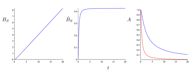
Figure 5: The average Ab concentration, $B_{S}$, and the rate $\dot{B}_{S}=\mathrm{d}B_{S}/\mathrm{d}t$ and (normalised) Ag $A$ (top blue curve: self-Ag; bottom red curve: target Ag), shown as functions of time $t$ for $A_{S}^{0}|\mathbf{r}^{S}|^{2}=10$, $\alpha=10$, $\beta=0.01$ and $\gamma=0.0009$.

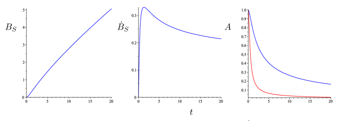
Figure 6: The average Ab concentration, $B_{S}$, and the rate $\dot{B}_{S}=\mathrm{d}B_{S}/\mathrm{d}t$ and (normalised) Ag $A$ (top blue curve: self-Ag; bottom red curve: target Ag), shown as functions of time $t$ for $A_{S}^{0}|\mathbf{r}^{S}|^{2}=10$, $\alpha=10$, $\beta=0.01$ and $\gamma=0.009$.

We solve equation [96] numerically in the regimes [103] and [109], for a given values of $\beta$ and $A_{S}^{0}|\mathbf{r}^{S}|^{2}$. The solutions are plotted in Figures 5–8. Also we compare the upper bound [106] with a typical solution of [96] in Figure 9.

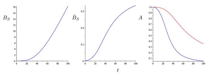
Figure 7: The average Ab concentrations , $B_{S}$, and the rate $\dot{B}_{S}$ and (normalised) Ag $A$ (top blue curve: self-Ag; bottom red curve: target Ag), shown as functions of time $t$ for $A_{S}^{0}|\mathbf{r}^{S}|^{2}=10$, $\alpha=1$, $\beta=0.01$ and $\gamma=0.009$.

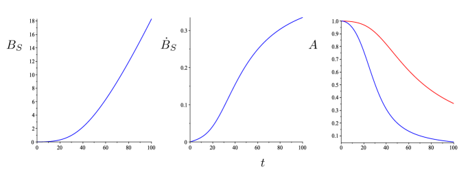
Figure 8: The average Ab concentrations, $B_{S}$, and the rate $\dot{B}_{S}$ and (normalised) Ag $A$ (top blue curve: self-Ag; bottom red curve: target Ag), shown as functions of time $t$ for $A_{S}^{0}|\mathbf{r}^{S}|^{2}=10$, $\alpha=0.1$, $\beta=0.01$ and $\gamma=0.009$.

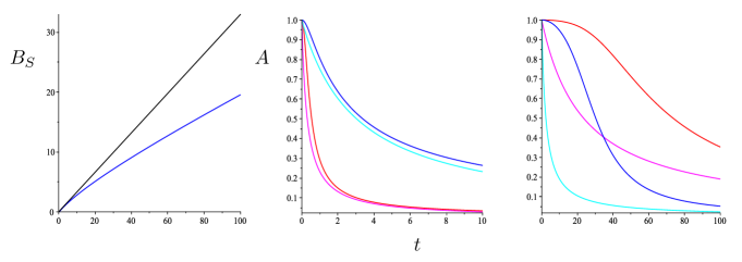
Figure 9: Left: The average of Ab concentrations , $B_{S}$, (blue line) and upper bound (black line) as a function of time $t$ for $\alpha=10$ and $\gamma=0.009$. Middle: The (normalised) Ag, $A$, (blue (cyan) curve is self-Ag and red (magenta) curve is target Ag) and the lower bound as a function of time $t$ for $\alpha=10$ and $\gamma=0.009$. Right: Ag and the lower bound (red (magenta) curve is target Ag and blue (cyan) curve is self-Ag) as a function of time $t$ for $\alpha=0.1$ and $\gamma=0.0009$. The $\beta=0.01$ and $A_{S}^{0}|\mathbf{r}^{S}|^{2}=10$.

Let us now consider the normalised damage per unit of time

$$\delta_{A}(t_{1}-t_{0}) = \frac{1}{A(\mathbf{b}(t_{0}))\left(t_{1}-t_{0}\right)}\int_{t_{0}}^{t_{1}}\!\mathrm{d}t^{\prime}\leavevmode\nobreak\ A(\mathbf{b}({t^{\prime}})),$$ (111)

where $0\leq\delta_{A}\leq 1$, and a similar integral

$$\delta_{S}(t_{1}-t_{0})=\frac{1}{A_{S}(\mathbf{b}(t_{0}))\left(t_{1}-t_{0}\right)}\int_{t_{0}}^{t_{1}}\!\mathrm{d}t^{\prime}\leavevmode\nobreak\ A_{S}(\mathbf{b}({t^{\prime}})),$$ (112)

where $0\leq\delta_{S}\leq 1$, which defines the (normalised) self-damage per unit of time $1-\delta_{S}$, where $0\leq 1-\delta_{S}\leq 1$. For the scenario described by the equation [96], on the time interval $[0,t]$, the above expressions give us

$$\delta_{A}(t)=\frac{1}{t}\int_{0}^{t}\!\mathrm{d}t^{\prime}\leavevmode\nobreak\ \frac{1}{1+\alpha B_{S}({t^{\prime}})},\leavevmode\nobreak\ \leavevmode\nobreak\ \leavevmode\nobreak\ \leavevmode\nobreak\ \leavevmode\nobreak\ \leavevmode\nobreak\ \leavevmode\nobreak\ \leavevmode\nobreak\ \leavevmode\nobreak\ \leavevmode\nobreak\ \delta_{S}(t)=\frac{1}{t}\int_{0}^{t}\!\mathrm{d}t^{\prime}\leavevmode\nobreak\ \frac{1}{1+B_{S}({t^{\prime}})}.$$ (113)

Since $1/(\!1+\!\alpha B)$ decreases monotonically with $B$, from $B_{S}(t)<t/\tau$ we obtain for the regime [103] the two lower bounds

$$\delta_{A}(t)\geq\delta_{A}^{*}(t)=\frac{\tau}{\alpha t}\log\left(1+\alpha\frac{t}{\tau}\right)\leavevmode\nobreak\ \leavevmode\nobreak\ \leavevmode\nobreak\ \leavevmode\nobreak\ \leavevmode\nobreak\ \leavevmode\nobreak\ \leavevmode\nobreak\ \leavevmode\nobreak\ \leavevmode\nobreak\ \leavevmode\nobreak\ \delta_{S}(t)\geq\delta_{S}^{*}(t)=\frac{\tau}{t}\log\left(1+\frac{t}{\tau}\right),$$ (114)

with the time constant

$$\tau^{-1} = \sqrt{2A_{S}^{0}|\mathbf{r}^{S}|^{2}\left(\beta-\gamma\right)},$$ (115)

Let us consider the function $\delta^{*}(x)=x^{-1}\log(1+x)$ for $x\in(0,\infty)$. Its derivative is ${\delta^{*}}^{\prime}(x)=[x-\left(1+x\right)\log\left(1+x\right)][\left(1+x\right)x^{2}]$. Due to the inequality $\log\left(1+x\right)\geq 1-(1+x)^{-1}$, this derivative is negative for any finite $x$, so $\delta^{*}(x)$ is a monotonic decreasing function with $\delta^{*}(x)\rightarrow 1$ as $x\rightarrow 0$ and $\delta^{*}(x)\rightarrow 0$ as $x\rightarrow\infty$. Since the image of $\delta^{*}(x)$ is the interval $[0,1]$ the function $1-\delta^{*}(x)$ is monotonic increasing on the same domain. It follows that $\delta_{A}^{*}(t)\rightarrow 1$ as $t\rightarrow 0$, implying that the (normalised) damage $\delta_{A}(t)\rightarrow 1$ in this limit, and $\delta_{A}^{*}(t)\rightarrow 0$ as $t\rightarrow\infty$. Also $1-\delta_{S}^{*}(t)\rightarrow 0$ as $t\rightarrow 0$, implying that the self-damage $1-\delta_{S}(t)\rightarrow 0$ in this limit, and $1-\delta_{S}^{*}(t)\rightarrow 1$ as $t\rightarrow\infty$. For $\alpha=1$ (where the strengths of antibody interaction with non-self and self are identical) we obtain $\delta_{A}^{*}=\delta_{S}^{*}$ and the damage $\delta_{A}^{*}$ (lower bound) is linearly related to the self-damage he self-damage $1-\delta_{S}^{*}$ (upper bound) via $\delta_{A}^{*}=1-(1-\delta_{S}^{*})$. For $\alpha<1$ (where the strength of antibody interaction with self is greater than the interaction with non-self) we obtain $\delta_{A}^{*}>1-(1-\delta_{S}^{*})$, so for a small reduction in the damage $\delta_{A}^{*}$ we find a large increase in the damage to self $1-\delta_{S}^{*}$. For $\alpha>1$ (where the strength of antibody interaction with non-self is greater than the interaction with self) we obtain $\delta_{A}^{*}<1-(1-\delta_{S}^{*})$, i.e. for a large reduction in $\delta_{A}^{*}$ we have a small increase in $1-\delta_{S}^{*}$.

We (re-)label the antibodies such that $\lambda_{1}\leq\lambda_{2}\leq\cdots\leq\lambda_{M}$. We define the mean and the variance of the binding strengths to self-antigen, $m(\mathbf{r}^{S})=M^{-1}\sum_{\mu=1}^{M}r^{S}_{\mu}$ and $\sigma^{2}(\mathbf{r}^{S})=M^{-1}\sum_{\mu=1}^{M}(r^{S}_{\mu})^{2}-(M^{-1}\sum_{\mu=1}^{M}r^{S}_{\mu})^{2}$, and consider $|\mathbf{r}^{S}|^{2}=M^{-1}\sum_{\mu=1}^{M}\lambda_{\mu}^{-1}(r^{S}_{\mu})^{2}$. We note that for $\lambda_{\mu}=\lambda$:

$$\lambda\,|\mathbf{r}^{S}|^{2} = \sigma^{2}(\mathbf{r}^{S})+m^{2}(\mathbf{r}^{S}),$$ (116)

Thus the time constant $\tau$ is given by

$$1/\tau(\lambda) = \sqrt{2A_{S}(\mathbf{0})\,\lambda^{-1}\left[\sigma^{2}(\mathbf{r}^{S})+m^{2}(\mathbf{r}^{S})\right]\left(\beta-\gamma\right)}$$ (117)

Second, the weighted average $M^{-1}\sum_{\mu=1}^{M}\lambda_{\mu}^{-1}\left(r^{S}_{\mu}\right)^{2}$, with $\lambda_{\mu}^{-1}\geq 0$ for all $\mu$, is bounded from below by $\lambda_{M}^{-1}M^{-1}\sum_{\mu=1}^{M}(r^{S}_{\mu})^{2}$ and from above by $\lambda_{1}^{-1}M^{-1}\sum_{\mu=1}^{M}(r^{S}_{\mu})^{2}$. Hence the time constant in [115] is bounded according to

$$\tau(\lambda_{1})\leq\tau(\lambda)\leq\tau(\lambda_{M})$$ (118)

This fact, in combination with the monotonicity of the $x^{-1}\log(1+x)$ as it appears in [114], gives us new lower bounds on the damage to non-self and the damage on self:

$$\delta_{A}(t)\geq\frac{\tau\left(\lambda_{1}\right)}{\alpha\,t}\log\Big{(}1+\alpha\,\frac{t}{\tau\left(\lambda_{1}\right)}\Big{)}\leavevmode\nobreak\ \leavevmode\nobreak\ \leavevmode\nobreak\ \leavevmode\nobreak\ \leavevmode\nobreak\ \leavevmode\nobreak\ \leavevmode\nobreak\ \leavevmode\nobreak\ \delta_{S}(t)\geq\frac{\tau\left(\lambda_{1}\right)}{t}\log\Big{(}1+\frac{t}{\tau\left(\lambda_{1}\right)}\Big{)}$$ (119)

We note that, since the time constant $\tau$ controls the speed of antigen removal, see equation [101], this speed is a monotonic increasing function of the variance $\sigma^{2}(\mathbf{r}^{S})$ and the mean $m(\mathbf{r}^{S})$ of the vector of affinities $\mathbf{r}^{S}$, i.e. of the antibody repertoire. Thus, having a repertoire with a higher variance facilitates a more rapid Ag removal.

References

- (1) Dunn-Walters D, Townsend C, Sinclair E, Stewart A (2018) Immunoglobulin gene analysis as a tool for investigating human immune responses. Immunological reviews 284(1):132–147.
- (2) Dunn-Walters DK (2016) The ageing human b cell repertoire: a failure of selection? Clinical & Experimental Immunology 183(1):50–56.
- (3) Dondelinger M, et al. (2018) Understanding the significance and implications of antibody numbering and antigen-binding surface/residue definition. Frontiers in immunology 9.
- (4) Martin VG, et al. (2016) Transitional b cells in early human b cell development–time to revisit the paradigm? Frontiers in immunology 7:546.
- (5) Childs LM, Baskerville EB, Cobey S (2015) Trade-offs in antibody repertoires to complex antigens. Philosophical Transactions of the Royal Society B: Biological Sciences 370(1676):20140245.
- (6) Wu YCB, Kipling D, Dunn-Walters DK (2012) Age-related changes in human peripheral blood igh repertoire following vaccination. Frontiers in immunology 3:193.
- (7) Poulsen TR, Meijer PJ, Jensen A, Nielsen LS, Andersen PS (2007) Kinetic, affinity, and diversity limits of human polyclonal antibody responses against tetanus toxoid. The Journal of Immunology 179(6):3841–3850.
- (8) Bannard O, Cyster JG (2017) Germinal centers: programmed for affinity maturation and antibody diversification. Current opinion in immunology 45:21–30.
- (9) Ademokun A, et al. (2011) Vaccination-induced changes in human b-cell repertoire and pneumococcal igm and iga antibody at different ages. Aging cell 10(6):922–930.
- (10) Goronzy JJ, Weyand CM (2019) Mechanisms underlying t cell ageing. Nature Reviews Immunology p. 1.
- (11) Martin V, Wu YC, Kipling D, Dunn-Walters D (2015) Ageing of the b-cell repertoire. Philosophical Transactions of the Royal Society B: Biological Sciences 370(1676):20140237.
- (12) Laffy JM, et al. (2017) Promiscuous antibodies characterised by their physico-chemical properties: From sequence to structure and back. Progress in biophysics and molecular biology 128:47–56.
- (13) Gibson KL, et al. (2009) B-cell diversity decreases in old age and is correlated with poor health status. Aging cell 8(1):18–25.
- (14) Kepler TB, Perelson AS (1993) Somatic hypermutation in b cells: An optimal control treatment. Journal of Theoretical Biology 164(1):37 – 64.
- (15) Agliari E, Barra A, Guerra F, Moauro F (2011) A thermodynamic perspective of immune capabilities. J. Theor. Biol. 287:48–63.
- (16) Bartolucci S, Annibale A (2015) A dynamical model of the adaptive immune system: effects of cells promiscuity, antigens and b b interactions. J. Stat. Mech. Theory Exp. 2015(8):P08017.
- (17) Mozeika A, Coolen ACC (2016) Statistical mechanics of clonal expansion in lymphocyte networks modelled with slow and fast variables. J. Phys. A: Math. Theor. 50(3):035602.
- (18) Theofilopoulos AN, Kono DH, Baccala R (2017) The multiple pathways to autoimmunity. Nature immunology 18(7):716.
- (19) Perelson AS, Oster GF (1979) Theoretical studies of clonal selection: minimal antibody repertoire size and reliability of self-non-self discrimination. Journal of theoretical biology 81(4):645–670.
- (20) De Boer RJ, Perelson AS (1993) How diverse should the immune system be? Proceedings of the Royal Society of London. Series B: Biological Sciences 252(1335):171–175.
- (21) Mayer A, Balasubramanian V, Mora T, Walczak AM (2015) How a well-adapted immune system is organized. P. Natl. Acad. Sci. USA 112(19):5950–5955.
- (22) Janeway C, Murphy KP, Travers P, Walport M (2012) Janeway’s Immunobiology. (Garland Science).
- (23) Arnold VI (1989) Mathematical methods of classical mechanics. (Springer).
- (24) Gelfand IM, Silverman RA, , et al. (2000) Calculus of variations. (Courier Corporation).
- (25) Yablonskii Gv, Bykov V, Elokhin V, Gorban A (1991) Kinetic models of catalytic reactions. (Elsevier) Vol. 32.
- (26) Gorban A, Yablonsky G (2011) Extended detailed balance for systems with irreversible reactions. Chemical Engineering Science 66(21):5388–5399.