Jump Markov Chains and

Rejection-Free Metropolis Algorithms

by

Jeffrey S. Rosenthal, Aki Dote^,, Keivan Dabiri²,

Hirotaka Tamura³, Sigeng Chen¹, and Ali Sheikholeslami²

(Version of )

Abstract. We consider versions of the Metropolis algorithm which avoid the inefficiency of rejections. We first illustrate that a natural Uniform Selection Algorithm might not converge to the correct distribution. We then analyse the use of Markov jump chains which avoid successive repetitions of the same state. After exploring the properties of jump chains, we show how they can exploit parallelism in computer hardware to produce more efficient samples. We apply our results to the Metropolis algorithm, to Parallel Tempering, to a Bayesian model, to a two-dimensional ferromagnetic 4$\times$4 Ising model, and to a pseudo-marginal MCMC algorithm.

1 Introduction

The Metropolis algorithm [15, 10] is a method of designing a Markov chain which converges to a given target density $\pi$ on a state space $S$. Such Markov chain Monte Carlo (MCMC) algorithms have become extremely popular in statistical applications and have led to a tremendous amount of research activity (see e.g. [3] and the many references therein).

The Metropolis algorithm produces a Markov chain $X_{0},X_{1},X_{2},\ldots$ on $S$, as follows. Given the current state $X_{n}$, the Metropolis algorithm first proposes a new state $Y_{n}$ from a symmetric proposal distribution $Q(X_{n},\cdot)$. It then accepts the new state (i.e., sets $X_{n+1}=Y_{n}$) with probability $\min\left(1,\ {\pi(Y_{n})\over\pi(X_{n})}\right)$, i.e. if $U_{n}<{\pi(Y_{n})\over\pi(X_{n})}$ where $U_{n}$ is an independent Uniform[0,1] random variable. Otherwise, it rejects the proposal (i.e., sets $X_{n+1}=X_{n}$). This simple algorithm ensures that the Markov chain has $\pi$ as a stationary distribution.

With this algorithm, the expected value ${\bf E}_{\pi}(h)$ of a function $h:S\to{\bf R}$ can then be estimated by the usual estimator, $\hat{e}_{K}={1\over K}\sum_{n=1}^{K}h(X_{n})$. The Strong Law of Large Numbers (SLLN) for Markov chains (e.g. [16, Theorem 17.0.1]) says that assuming that ${\bf E}_{\pi}(h)$ is finite, and that the Markov chain is irreducible with stationary distribution $\pi$, we must have $\lim_{K\to\infty}\hat{e}_{K}={\bf E}_{\pi}(h)$, i.e. this estimate $\hat{e}_{K}$ is consistent. For example, if $h={\bf 1}_{A}$ is the indicator function of an event $A$, then $\lim_{K\to\infty}\hat{e}_{K}={\bf P}(A)$. Or, if $h=g^{k}$ is a power of some other function $g$, then $\lim_{K\to\infty}\hat{e}_{K}={\bf E}_{\pi}(h)={\bf E}_{\pi}(g^{k})$. Consistency is thus a useful property which guarantees asymptotically accurate estimates of any quantity of interest.

One problem with the Metropolis algorithm is that it might reject many proposals, leading to inefficiencies in its convergence. Indeed, in certain contexts the optimal Metropolis algorithm should reject over three quarters of its proposals [17, 18]. Each rejection involves sampling a proposed state, computing a ratio of target probabilities, and deciding not to accept the proposal, only to remain at the current state. These rejections are normally considered to be a necessary evil of the Metropolis algorithm. However, recent technological advances have allowed for exploiting parallelism in computer hardware, computing all potential acceptance probabilities at once, thus allowing for the possibility of skipping the rejection steps and instead accepting a move every time. Such rejection-free algorithms can be very efficient, but they must be executed correctly or they can lead to biased estimates, as we now explore.

2 The Uniform Selection Algorithm

A first try at a rejection-free Metropolis algorithm might be as follows. Suppose that from a state $x$, one of a (large, finite) collection of states $y_{1},y_{2},\ldots,y_{k}$ (all distinct from $x$) would have been proposed uniformly at random. Then, sample $U\sim\textrm{Uniform}[0,1]$, and consider the sub-collection of states $C:=\{y_{i}:U<\pi(y_{i})/\pi(x)\}$ that “would” have been accepted, and then pick one of the states in $C$ uniformly at random. (If $C$ happens to be empty, then we immediately re-sample $U$ and try again. Technically speaking, that would be a “rejection”, though its probability is small.) This algorithm will always move somewhere, so there is no rejection. However, this algorithm is different from true MCMC, and might not converge to $\pi$, as we now show.

Example 1: Suppose the state space $S=\{1,2,3\}$, with $\pi(1)=1/2$, $\pi(2)=1/3$, and $\pi(3)=1/6$, as in Figure 1, and suppose that from each state $x$, the chain proposes to move either to $x-1$ or to $x+1$ with probability 1/2 each (where proposals to 0 or to 4 are always rejected).

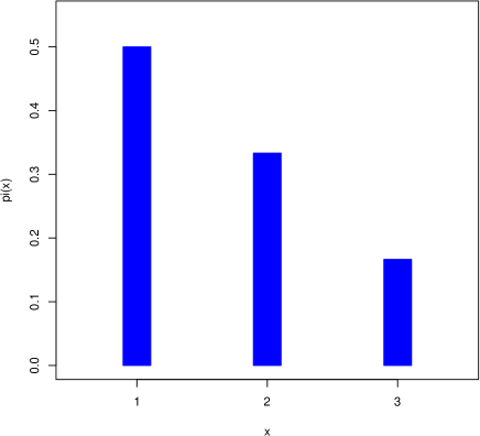
Figure 1: The target distribution for Example 1.

In this example, the Metropolis algorithm would have Markov chain transition probabilities as in Figure 2, which are easily computed to have the correct limiting stationary distribution $\pi=(1/2,1/3,1/6)$ as they must.

Figure 2: The Metropolis chain for Example 1.

However, the Uniform Selection algorithm would have Markov chain transition probabilities as in Figure 3, with limiting stationary distribution easily computed to instead be $(3/5,4/15,2/15)$ which is significantly different. For example, from state 2, the usual Metropolis algorithm would accept a proposed move to state 1 with probability 1, and would accept a proposed move to state 3 with probability $(1/6)\,/\,(1/3)=1/2$, so it would be twice as likely to move to state 1 as to move to state 3. But for the above Uniform Selection version, if $U>1/2$ then the subset $C$ would consist of just the single state 1 so it would always move to state 1, or if $U<1/2$ then the subset $C$ would consist of the two states 1 and 3 so it would move to state 1 or state 3 with probability 1/2 each, so overall it would move to state 1 with probability $(1/2)(1)+(1/2)(1/2)=3/4$ or to state 3 with probability $(1/2)(0)+(1/2)(1/2)=1/4$, i.e. it would now be three times as likely to move to state 1 as to move to state 3, not twice. This illustrates that this Uniform Selection algorithm will converge to the wrong distribution, i.e. it will fail to converge to the correct target distribution. ∎

Figure 3: The Uniform Selection chain for Example 1.

Our second example shows that Uniform Selection can even cause a Markov chain to become transient.

Example 2: Suppose now that the state space is the set $S=\{0,1,2,3,\ldots\}$ of all non-negative integers, with target distribution $\pi$ defined by writing the argument $x$ as $x=4a+b$ where $0\leq b\leq 3$ is the remainder upon dividing $x$ by 4, and defining (see Figure 4)

$$\pi(x)\ =\ \pi(4a+b)\ =\ {1\over 135}\,(8/9)^{a}\,2^{b}\,,\quad 0\leq b\leq 3,\quad a=0,1,2,\ldots$$

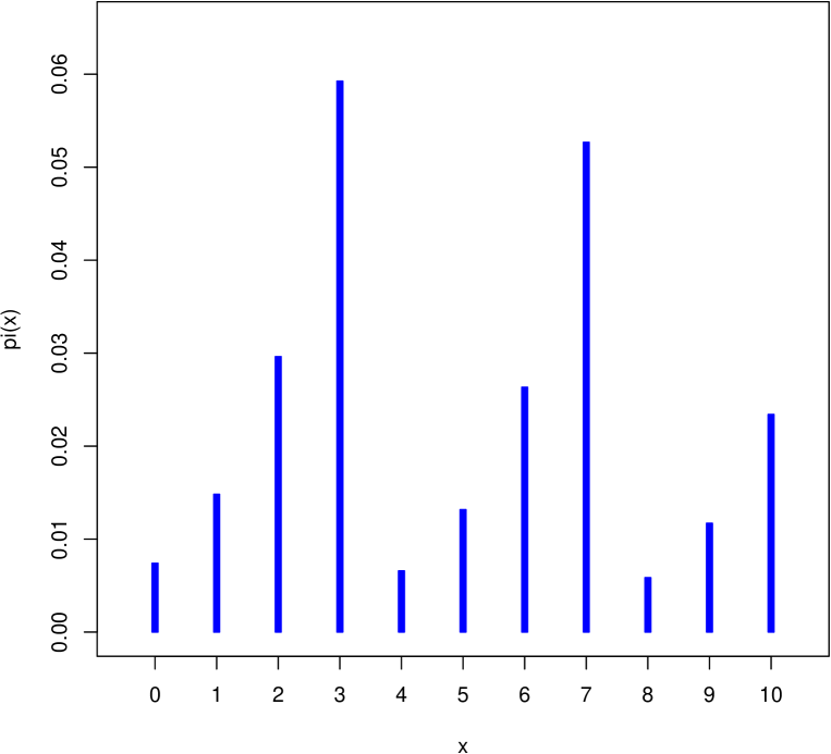
Figure 4: Part of the target distribution for Example 2.

As a check,

$$\sum_{x=0}^{\infty}\pi(x)\ =\ \sum_{a=0}^{\infty}{1\over 135}\,(8/9)^{a}\,(2^{0}+2^{1}+2^{2}+2^{3})\ =\ {1\over 135}\,\left(1\over 1-(8/9)\right)\,(15)\ =\ 1\,,$$

i.e. $\pi$ is a valid probability distribution. The Metropolis algorithm chain for this example is given by Figure 5, and it has the correct limiting stationary distribution $\pi$, as it must.

Figure 5: The Metropolis chain for Example 2.

However, the Uniform Selection chain is instead given by Figure 6. We prove in the Appendix that this Uniform Selection chain is transient, and in fact:

Proposition 1.

If the Uniform Selection chain for Example 2 begins at state $4a$ for some positive integer $a\geq 2$, then the probability it will ever reach the state 3 is $\leq(8/9)^{a-1}<1$.

That is, the Uniform Selection chain might fail to ever reach the optimal value. For example, if $X_{0}=100$, then $a=25$ and the probability of failure is at least $1-(8/9)^{24}>0.94=94\%$. This is also illustrated by the simulation in Figure 7 with initial state $X_{0}=100$. ∎

These examples show that the Uniform Selection algorithm may converge to the wrong limiting distribution, and thus should not be used for sampling purposes.

Example 2 also has implications for optimisation. Any Markov chain which gives consistent estimators can be used to find the mode (maximum value) of $\pi$, either by running the chain for a long time and taking its empirical sample mode, or by keeping track of the largest value $\pi(x)$ over all samples visited. However, Example 2 shows that a Uniform Selection chain could be transient and thus fail to find or converge to the maximum value at all. Of course, if the state space $S$ is required to be finite, then any irreducible chain will eventually find the optimal value. However, the time to find it could be extremely large. Indeed, the Appendix also shows that if Example 2 is instead truncated at a large value $4L$, then each attempt from $4L$ to reach state 3 before returning to $4L$ would have probability less than $(8/9)^{L-1}$ of success. Hence, the expected time to ever reach the state 3 would be exponentially large as a function of $L$, and the chain would still spend nearly all of its time very near to the state $4L$, so its samples and sample mean and sample mode would all be extremely far from the true optimal state 3.

Figure 6: The Uniform Selection chain for Example 2.

Figure 7: Output from the Uniform Selection chain for Example 2.

3 The Jump Chain

Due to the problems with the Uniform Selection Algorithm identified above, we instead turn attention to a more promising avenue, the Jump Chain. Our definitions are as follows.

Let $\{X_{n}\}$ be an irreducible Markov chain on a state space $S$ (the “original chain”). For ease of exposition we initially assume that $S$ is finite or countable, though we later (Theorem 13) extend this to general Markov chains with densities. To avoid trivialities, we assume throughout that $|S|>1$.

Given a run $\{X_{n}\}$ of the Markov chain, we define the Jump Chain $\{J_{k}\}$ to be the same chain except omitting any immediately repeated states, and the Multiplicity List $\{M_{k}\}$ to count the number of times the original chain remains at the same state. For example, if the original chain $\{X_{n}\}$ began

$$\{X_{n}\}=(a,b,b,b,a,a,c,c,c,c,d,d,a,\ldots)\,,$$

then the jump chain $\{J_{k}\}$ would begin

$$\{J_{k}\}=(a,b,a,c,d,a,\ldots)\,,$$

and the corresponding multiplicity list $\{M_{k}\}$ would begin

$$\{M_{k}\}=(1,3,2,4,2,\ldots)\,.$$

The concept of jump chains arises frequently for Markov processes, especially for continuous-time processes where they are often defined in terms of infinitesimal generators; see e.g. Section 4.4 of [7] or Proposition 4.4.20 of [21]. Here we develop the essential properties that we will use below. Most of these properties are already known in the context of (reversible) Metropolis-Hastings algorithms; see Remark 6 below.

To continue, let

$$P(y|x)\ =\ {\bf P}[X_{n+1}=y\,|\,X_{n}=x]\,,\quad x,y\in S$$

be the transition probabilities for the original chain $\{X_{n}\}$. And, let

$$\alpha(x)\ =\ {\bf P}[X_{n+1}\not=x\,|\,X_{n}=x]\ =\ \sum_{y\not=x}P(y|x)\ =\ 1-P(x|x)$$ (1)

be the “escape” probability that the original chain will move away from $x$ on the next step. Note that since the chain is irreducible and $|S|>1$, we must have $\alpha(x)>0$ for all $x\in S$. We then verify the following properties of the jump chain.

Proposition 2.

The jump chain $\{J_{k}\}$ is itself a Markov chain, with transition probabilities $\widehat{P}(y|x)$ specified by $\widehat{P}(x|x)=0$, and for $y\not=x$,

$$\widehat{P}(y|x)\ :=\ {\bf P}[J_{k+1}=y\,|\,J_{k}=x]\ =\ {P(y|x)\over\sum_{z\not=x}P(z|x)}\ =\ {P(y|x)\over\alpha(x)}\,.$$ (2)

Proof.

It follows from the definition of $\{J_{k}\}$ that $\widehat{P}(x|x)=0$. For $x,y\in S$ with $y\not=x$, we compute that

$$\widehat{P}(y|x)\ =\ {\bf P}[J_{k+1}=y\,\bigm{|}\,J_{k}=x]\ =\ {\bf P}[X_{n+1}=y\,\bigm{|}\,X_{n}=x,\ X_{n+1}\not=X_{n}]$$

$$\ =\ {{\bf P}[X_{n+1}=y,\ X_{n+1}\not=X_{n}\,\bigm{|}\,X_{n}=x]\over{\bf P}[X_{n+1}\not=X_{n}\,\bigm{|}\,X_{n}=x]}\ =\ {P(y|x)\over\sum_{z\not=x}P(z|x)}\,,$$

as claimed. ∎

Proposition 3.

The conditional distribution of $M_{k}$ given $J_{k}$ is equal to the distribution of $1+G$ where $G$ is a geometric random variable with success probability $p=\alpha(J_{k})$, i.e.

$${\bf P}[M_{k}=m\,\bigm{|}\,J_{k}]=(1-p)^{m-1}p=(1-\alpha(J_{k}))^{m-1}\alpha(J_{k})\,,\quad m=1,2,\ldots\,,$$ (3)

and furthermore ${\bf E}[M_{k}\,|\,J_{k}]=1/p=1/\alpha(J_{k})$.

Proof.

If the original chain is at state $x$, then it has probability $p=\alpha(x)$ of leaving $x$ on the next step, or probability $1-\alpha(x)$ of remaining at $x$. Hence, the probability that it will remain at $x$ for $m$ steps total (i.e., $m-1$ additional steps), and then leave at the next step, is equal to $(1-p)^{m-1}p$, as claimed. ∎

Proposition 4.

If the original chain $P$ is irreducible, then so is the jump chain $\widehat{P}$.

Proof.

Let $x,y\in S$. Since $P$ is irreducible, there is a path $x=x_{0},x_{1},x_{2},\ldots,x_{m}=y$ with $P(x_{i+1}|x_{i})>0$ for all $i$. Without loss of generality, we can assume the $\{x_{i}\}$ are all distinct. But if $P(x_{i+1}|x_{i})>0$, then (2) implies that also $\widehat{P}(x_{i+1}|x_{i})>0$. Hence, $\widehat{P}$ is also irreducible. ∎

Proposition 5.

If the original chain $P$ has stationary distribution $\pi$, then the jump chain $\widehat{P}$ has stationary distribution $\widehat{\pi}$ given by $\widehat{\pi}(x)=c\,\alpha(x)\,\pi(x)$ where $c=\Big{(}\sum_{y}\alpha(y)\,\pi(y)\Big{)}^{-1}$.

Proof.

Recall that on a discrete space, $\pi$ is stationary for $P$ if and only if $\sum_{x}\pi(x)\,P(y|x)=\pi(y)$ for all $y\in S$. In that case, we compute that

$$\sum_{x}\widehat{\pi}(x)\,\widehat{P}(y|x)\ =\ \sum_{x}\left(c\,\alpha(x)\,\pi(x)\right)\left([{P(y|x)/\alpha(x)}]\,{\bf 1}_{y\not=x}\right)$$

$$\ =\ c\,\sum_{x\not=y}\pi(x)\,P(y|x)\ =\ c\,\left(\sum_{x}\pi(x)\,P(y|x)\right)-c\,\pi(y)\,P(y|y)$$

$$\ =\ c\,\pi(y)-c\,\pi(y)\,P(y|y)\ =\ c\,\pi(y)[1-P(y|y)]\ =\ c\,\pi(y)\,\alpha(y)\ =\ \widehat{\pi}(y)\,,$$

so that $\widehat{\pi}$ is stationary for $\widehat{P}$, as claimed. ∎

Remark 6.

Most of the results presented in this section are already known in the Metropolis-Hastings (reversible) context: the geometric distribution of the holding times is noted in Lemma 1(3) of [5] and Proposition 1(a) of [11]; the modified transition probabilities of the jump chain are stated in Proposition 1(b) of [11]; and the relationship between the stationary distributions of the original and jump chains is used in Lemma 1(4) of [5], Proposition 1(c) of [11] (see also Proposition 2.1 of [14]), Lemma 1 of [6], and Section 2 of [4].

Remark 7.

It is common that simple modifications of reversible chains lead to simple modifications of their stationary distributions. For example, if a reversible chain is restricted to a subset of the state space (so any moves out of the subset are rejected with the chain staying where it is), then its stationary distribution is equal to the original stationary distribution conditional on being in that subset (since the detailed balance equation still holds on the subset). However, that property does not hold without reversibility. For a simple counter-example, let $S=\{1,2,3\}$, with $P(2|1)=P(3|2)=P(1|3)=3/4$, and $P(3|1)=P(1|2)=P(2|3)=1/4$. Then if $C=\{1,2\}$, then the stationary distribution of the original chain is $(1/3,1/3,1/3)$, but the stationary distribution of the chain restricted to $C$ is $(1/4,3/4)$. We were thus surprised that Proposition 5 holds even for non-reversible chains.

4 Using the Jump Chain for Estimation

The Jump Chain can be used for estimation, as we now discuss. This approach has also been taken by others; see Remarks 9 and 14 below.

Theorem 8.

Given an irreducible Markov chain $\{X_{n}\}$ with transition probabilities $P(y|x)$ and stationary distribution $\pi$ on a state space $S$, and a function $h:S\to{\bf R}$, suppose we simulate the jump chain $\{J_{k}\}$ with the transition probabilities (2), and then simulate the multiplicities list $\{M_{k}\}$ from the conditional probabilities (3) where $p=\alpha(J_{k})$ with $\alpha$ as in (1), and set

$$\bar{e}_{L}\ =\ {\sum_{k=1}^{L}M_{k}\,h(J_{k})\over\sum_{k=1}^{L}M_{k}}\,.$$ (4)

Then $\bar{e}_{L}$ is a consistent estimator of the expected value ${\bf E}_{\pi}(h)$, i.e. $\lim\limits_{L\to\infty}\bar{e}_{L}={\bf E}_{\pi}(h)$ w.p. 1.

Proof.

Recall (e.g. [16]) that the usual estimator $\hat{e}_{K}={1\over K}\sum_{n=1}^{K}h(X_{n})$ is consistent, i.e. $\lim_{K\to\infty}\hat{e}_{K}={\bf E}_{\pi}(h)$ w.p. 1. Then, it is seen that

$$\bar{e}_{L}\ =\ {\sum_{k=1}^{L}M_{k}\,h(J_{k})\over\sum_{k=1}^{L}M_{k}}\ =\ \hat{e}_{\sum_{k=1}^{L}M_{k}}\ =\ \hat{e}_{K(L)}$$

where $K(L)=\sum_{k=1}^{L}M_{k}$. Since each $M_{k}\geq 1$, $\lim_{L\to\infty}K(L)=\infty$, so $\lim_{L\to\infty}\bar{e}_{L}=\lim_{L\to\infty}\hat{e}_{K(L)}=\lim_{K\to\infty}\hat{e}_{K}={\bf E}_{\pi}(h)$ w.p. 1, as claimed. ∎

Remark 9.

The consistency of the estimate (4), and similarly those of Theorems 12 and 13 below, is already known in the Metropolis-Hastings (reversible) context; see equation (3) of [14], Section 2 of [5], and equation (2) of [11].

On the other hand, combining the Markov chain Law of Large Numbers with Propositions 4 and 5 immediately gives:

Proposition 10.

Under the above assumptions, if we simulate the jump chain $\{J_{k}\}$ with the transition probabilities $\widehat{P}$, then for any function $g:S\to{\bf R}$ with $\widehat{\pi}|g|<\infty$, we have

$$\lim_{L\to\infty}{1\over L}\sum_{k=1}^{L}g(J_{k})\ =\ \widehat{\pi}(g)\ :=\ \sum_{x\in S}g(x)\,\widehat{\pi}(x)\ =\ c\,\sum_{x\in S}g(x)\,\alpha(x)\,\pi(x)\ \ w.p.~{}1.$$

Corollary 11.

Under the above assumptions, if we simulate the jump chain $\{J_{k}\}$ with the transition probabilities $\widehat{P}$, then for any function $h:S\to{\bf R}$ with $\pi|h|<\infty$, we have

$$\lim_{L\to\infty}{1\over c\,L}\sum_{k=1}^{L}[h(J_{k})/\alpha(J_{k})]\ =\ \pi(h)\ :=\ \sum_{x\in S}h(x)\,\pi(x)\,,\ \ w.p.~{}1.$$

Proof.

Let $g(x)=h(x)/c\,\alpha(x)$. Then since $\pi|h|<\infty$, we have

$$\widehat{\pi}|g|\ =\ \sum_{x}|g(x)|\,\widehat{\pi}(x)\ =\ \sum_{x}[|h(x)|/c\,\alpha(x)]\,c\,\alpha(x)\,\pi(x)\ =\ \sum_{x}|h(x)|\,\pi(x)\ =\ \pi|h|\ <\ \infty\,.$$

So, the result follows upon plugging this $g$ into Proposition 10. ∎

We then have:

Theorem 12.

Under the above assumptions, if we simulate the jump chain $\{J_{k}\}$ with the transition probabilities $\widehat{P}$, then for any function $h:S\to{\bf R}$ with $\pi|h|<\infty$, we have

$$\lim_{L\to\infty}{\sum_{k=1}^{L}[h(J_{k})/\alpha(J_{k})]\over\sum_{k=1}^{L}[1/\alpha(J_{k})]}\ =\ \pi(h)\,,\ \ w.p.~{}1.$$ (5)

Proof.

Setting $h\equiv 1$ in Corollary 11 gives that w.p. 1, $\lim_{L\to\infty}{1\over c\,L}\sum_{k=1}^{L}[1/\alpha(J_{k})]\,=\,1$. We then compute that

$$\lim_{L\to\infty}{\sum_{k=1}^{L}[h(J_{k})/\alpha(J_{k})]\over\sum_{k=1}^{L}[1/\alpha(J_{k})]}\ =\ \lim_{L\to\infty}{{1\over cL}\sum_{k=1}^{L}[h(J_{k})/\alpha(J_{k})]\over{1\over cL}\sum_{k=1}^{L}[1/\alpha(J_{k})]}\ =\ {\sum_{x\in S}h(x)\,\pi(x)\over 1}\ =\ \pi(h)\,,$$

as claimed. ∎

Comparing Theorems 8 and 12, we see that they coincide except that each multiplicity random variable $M_{k}$ has been replaced by its mean $1/\alpha(J_{k})$, cf. Proposition 3.

Finally, we note that although our computer hardware does not allow us to exploit it, most of the above carries over to Markov chains with densities on general (continuous) state spaces, as follows. (The proofs are very similar to the discrete case, and are thus omitted.)

Theorem 13.

Let ${\cal X}$ be a general state space, and $\mu$ an atomless $\sigma$-finite reference measure on ${\cal X}$. Suppose a Markov chain on ${\cal X}$ has transition probabilities $P(x,dy)=r(x)\,\delta_{x}(dy)+\rho(x,y)\,\mu(dy)$ for some $r:{\cal X}\to[0,1]$ and $\rho:{\cal X}\times{\cal X}\to[0,\infty)$ with $r(x)+\int\rho(x,y)\,\mu(dy)=1$ for each $x\in{\cal X}$, where $\delta_{x}$ is a point-mass at $x$. Again let $\widehat{P}$ be the transitions for the corresponding jump chain $\{J_{k}\}$ with multiplicities $\{M_{k}\}$. Then: (i) $\widehat{P}(x,\{x\})=0$,  and for $x\not=y$,  $\widehat{P}(x,dy)={\rho(x,y)\over\int\rho(x,z)\,\mu(dz)}\mu(dy)$. (ii) The conditional distribution of $M_{k}$ given $J_{k}$ is equal to the distribution of $1+G$ where $G$ is a geometric random variable with success probability $p=\alpha(J_{k})$ where $\alpha(x)={\bf P}[X_{n+1}\not=x\,|\,X_{n}=x]=\int\rho(x,z)\,\mu(dz)=1-r(x)=1-P(x|x)$. (iii) If the original chain is $\phi$-irreducible (see e.g. [16]) for some positive $\sigma$-finite measure $\phi$ on ${\cal X}$, then the jump chain is also $\phi$-irreducible for the same $\phi$. (iv) If the original chain has stationary distribution $\pi(x)\,\mu(dx)$, then the jump chain has stationary distribution given by $\widehat{\pi}(x)=c\,\alpha(x)\,\pi(x)\,\mu(dx)$ where $c^{-1}=\int\alpha(y)\,\pi(y)\,\mu(dy)$. (v) If $h:{\cal X}\to{\bf R}$ has finite expectation, then with probability 1,

$$\lim\limits_{L\to\infty}{\sum_{k=1}^{L}M_{k}\,h(J_{k})\over\sum_{k=1}^{L}M_{k}}\ =\ \lim\limits_{L\to\infty}{\sum_{k=1}^{L}[h(J_{k})/\alpha(J_{k})]\over\sum_{k=1}^{L}[1/\alpha(J_{k})]}\ =\ \pi(h)\ :=\ \int h(x)\,\pi(x)\,\mu(dx)\,.$$

4.1 Application to the Metropolis Algorithm

Suppose now that the original chain $\{X_{n}\}$ is a Metropolis algorithm, with proposal probabilities $Q(y|x)$ which are symmetric (i.e. $Q(y|x)=Q(x|y)$). Then for $x\not=y$, $P(y|x)=Q(y|x)\,\min\Big{(}1,\ {\pi(y)\over\pi(x)}\Big{)}$. Hence, by (2), the jump chain transition probabilities have $\widehat{P}(x|x)=0$ and for $x\not=y$ are given by

$$\widehat{P}(y|x)\ :=\ {\bf P}[J_{1}=y\,|\,J_{0}=x]\ =\ {Q(y|x)\,\min\Big{(}1,\ {\pi(y)\over\pi(x)}\Big{)}\over\sum_{z\not=x}Q(z|x)\,\min\Big{(}1,\ {\pi(z)\over\pi(x)}\Big{)}}\,.$$ (6)

Also, here

$$\alpha(x)\ =\ \sum_{y\not=x}P(y|x)\ =\ \sum_{y\not=x}Q(y|x)\,\min\Big{(}1,\ {\pi(y)\over\pi(x)}\Big{)}\,.$$ (7)

A special case is where the proposal probabilities $Q(x,\cdot)$ are uniform over all “neighbours” of $x$, where each state has the same number $N$ of neighbours. We assume that $x$ is not a neighbour of itself, and that $x$ is a neighbour of $y$ if and only if $y$ is a neighbour of $x$. Then for $x\not=y$, $P(y|x)={1\over N}\,\min\Big{(}1,\ {\pi(y)\over\pi(x)}\Big{)}$. And, by (2), the jump chain transition probabilities have $\widehat{P}(x|x)=0$ and for $x\not=y$ are given by

$$\widehat{P}(y|x)\ =\ {\min\Big{(}1,\ {\pi(y)\over\pi(x)}\Big{)}\over\sum_{z\sim x}\min\Big{(}1,\ {\pi(z)\over\pi(x)}\Big{)}}$$ (8)

where the sum is over all neighbours $z$ of $x$. Also, here

$$\alpha(x)\ =\ {1\over N}\,\sum_{y\not=x}\min\Big{(}1,\ {\pi(y)\over\pi(x)}\Big{)}\,.$$ (9)

The use of the estimators (4) and (5) in the context of uniform Metropolis algorithms can be carried out very efficiently using special parallelised computer hardware (see e.g. Section 7 below), and was our original motivation for this investigation.

Remark 14.

The “$n$-fold way” of Bortz et al. [2] considers the Ising model, and selects the next site to flip proportional to its probability of flipping, by first classifying all sites in terms of their spin and neighbour counts. This creates a rejection-free Metropolis-Hastings algorithm in the same spirit as our approach, though specific to the Ising model. Later authors parallelised their algorithm, still for the Ising model; see e.g. [13] and [12].

5 Alternating Chains

Sometimes we have two or more different Markov chains and we wish to alternate between them in some pattern. And, we might wish to use rejection-free sampling for some or all of the individual chains. However, if this is done naively, it can lead to bias:

Example 3: Let $S=\{1,2,3,4\}$, and $\pi=(1-\epsilon,3\epsilon,1-\epsilon,1-\epsilon)/3$ for some small positive number $\epsilon$ (e.g. $\epsilon=0.001$). Let $Q_{1}(x,\,x+1)=Q_{1}(x,\,x-1)=1/2$ and $Q_{2}(x,\,x+1)=Q_{2}(x,\,x+2)=Q_{2}(x,\,x-1)=Q_{2}(x,\,x-2)=1/4$ be two different proposal kernels, and let $P_{1}$ and $P_{2}$ be usual Metropolis algorithms for $\pi$ with proposals $Q_{1}$ and $Q_{2}$ respectively. Then, each of $P_{1}$ and $P_{2}$ will converge to $\pi$, as will the algorithm of alternating between $P_{1}$ and $P_{2}$ any fixed number of times. However, if we instead alternate between doing one jump step of $P_{1}$ and then one jump step of $P_{2}$, then this combined chain will not converge to the correct distribution. Indeed, the corresponding escape probabilities $\alpha_{1}(x)$ and $\alpha_{2}(x)$ are all reasonably large (at least 1/4) except for $\alpha_{1}(1)=\epsilon/2$ which is extremely small. This means that when our algorithm uses $P_{1}$ from state 1 then it will have an extremely large multiplicity $M_{k}$ which will lead to extremely large weight of the state 1. Indeed, if we use the alternating jump chains algorithm, then the estimators $\bar{e}_{L}$ as in (4) will have the property that as $\epsilon\searrow 0$, their limiting value converges to $h(1)$ instead of $\pi(h)$, i.e.

$$\lim_{\epsilon\searrow 0}\lim_{L\to\infty}\bar{e}_{L}\ =\ h(1)\,.$$

Hence, convergence to $\pi$ fails in this case. ∎

However, this convergence problem can be fixed if we control the number of effective repetitions of each kernel. Specifically, suppose we choose in advance some number $L_{0}$ of effective repetitions we wish to perform for the kernel $P_{1}$ before switching to the kernel $P_{2}$. Then we can do this in a rejection-free manner as follows:

1.  Set the number of remaining repetitions, $L$, equal to some fixed initial value $L_{0}$.

2.  Find the next jump chain value $J_{k}$ and multiplicity $M_{k}$ corresponding to the Markov chain $P_{1}$, as above.

3.  If $M_{k}\geq L$, then replace $M_{k}$ by $L$, and keep $J_{k}$ as it is, and include that $J_{k}$ and $M_{k}$ in the estimate. Then, return to step 1 with the next kernel $P_{2}$.

4.  Otherwise, if $M_{k}<L$, then keep $M_{k}$ and $J_{k}$ as they are, and count them in the estimate, and then replace $L$ by $L-M_{k}$ and return to step 2 with the same kernel $P_{1}$.

This modified algorithm is equivalent to applying the original (non-rejection-free) kernel $P_{1}$ a total of $L_{0}$ times before switching to the next kernel $P_{2}$. As such, it has no bias, and is consistent and will converge to the correct distribution without any errors as in the counter-example above.

6 Application to Parallel Tempering

Parallel tempering (or, replica exchange) [22, 9] proceeds by considering different versions of the target distribution $\pi$ powered by different inverse-temperatures $\beta$, of the form $\pi^{(\beta)}(x)\propto\big{(}\pi(x)\big{)}^{\beta}$. It runs separate MCMC algorithms on each target $\pi^{(\beta)}$, for some fixed number of iterations, and then proposes to “swap” pairs of values $X^{(\beta_{1})}\leftrightarrow X^{(\beta_{2})}$. This swap proposal is accepted with the usual Metropolis algorithm probability

$$\min\left[1,\ {\pi^{(\beta_{1})}(X^{(\beta_{2})})\,\pi^{(\beta_{2})}(X^{(\beta_{1})})\over\pi^{(\beta_{1})}(X^{(\beta_{1})})\,\pi^{(\beta_{2})}(X^{(\beta_{2})})}\right]$$ (10)

which preserves the product target measure $\prod_{\beta}\pi^{(\beta)}$.

But suppose we instead want to run parallel tempering using jump chains, i.e. using a rejection-free algorithm within each temperature. If we run a fixed number of rejection-free moves of each within-temperature chain, followed by one “usual” swap move, then this can lead to bias, as the following example shows.

Example 4: Let $S=\{1,2,3\}$, with $\pi(1)=\pi(3)=1/4$ and $\pi(2)=1/2$. Suppose there are just two inverse-temperature values, $\beta_{0}=1$ and $\beta_{1}=5$. Suppose each within-temperature chain proceeds as a Metropolis algorithm, with proposal distribution given by $Q(y|x)=1/2$ whenever $y\not=x$. (That is, we can regard the three states of $S$ as being in a circle, and the chain proposes to move one step clockwise or counter-clockwise with probability 1/2 each, and then accepts or rejects this move according to the usual Metropolis procedure.) If we run a usual parallel tempering algorithm, then the within-temperature moves will converge to the corresponding stationary distributions $\pi^{(0)}=\pi=(1/4,1/2,1/4)$ and $\pi^{(5)}=(1/34,32/34,1/34)$ respectively. Then, given current chain values $X^{(0)}$ and $X^{(5)}$, if we attempt a usual swap move, it will be accepted with probability

$$\min\left[1,\ {\pi^{(0)}(X^{(5)})\ \pi^{(5)}(X^{(0)})\over\pi^{(0)}(X^{(0)})\ \pi^{(5)}(X^{(5)})}\right]\,.$$ (11)

These steps will all preserve the product stationary distribution $\pi^{(0)}\times\pi^{(5)}$, as they should. However, if we instead run a rejection-free within-temperature chain, then convergence fails. Indeed, from each state the jump chain is equally likely to move to either of the other two states, so each jump chain will converge to the uniform distribution on $S$. The acceptance probability (11) will then lead to incorrect distributional convergence, e.g. if $X^{(0)}=2$ and $X^{(5)}=3$, then a proposal to swap $X^{(0)}$ and $X^{(5)}$ will always be accepted, leading to an excessively large probability that $X^{(0)}=3$. Indeed, in simulations the fraction of time that $X^{(0)}=3$ right after a swap proposal is about 44%, much larger than the 1/3 probability it should be. ∎

To get rejection-free parallel tempering to converge correctly, we recall from Proposition 5 that the rejection-free chains actually converge to the modified stationary distributions $\widehat{\pi}$, not $\pi$. We should thus modify the acceptance probability (10) to:

$$\min\left[1,\ {\widehat{\pi}^{(\beta_{1})}(X^{(\beta_{2})})\ \widehat{\pi}^{(\beta_{2})}(X^{(\beta_{1})})\over\widehat{\pi}^{(\beta_{1})}(X^{(\beta_{1})})\ \widehat{\pi}^{(\beta_{2})}(X^{(\beta_{2})})}\right]\qquad\qquad\qquad\qquad\qquad\qquad\qquad\qquad$$

$$\ =\ \min\left[1,\ {\alpha^{(\beta_{1})}(X^{(\beta_{2})})\ \pi^{(\beta_{1})}(X^{(\beta_{2})})\ \alpha^{(\beta_{2})}(X^{(\beta_{1})})\ \pi^{(\beta_{2})}(X^{(\beta_{1})})\over\alpha^{(\beta_{1})}(X^{(\beta_{1})})\ \pi^{(\beta_{1})}(X^{(\beta_{1})})\ \alpha^{(\beta_{2})}(X^{(\beta_{2})})\ \pi^{(\beta_{2})}(X^{(\beta_{2})})}\right]\,.$$ (12)

Such swaps will preserve the product modified stationary distribution $\prod_{\beta}\widehat{\pi}^{(\beta)}$, rather than trying to preserve the unmodified stationary distribution $\prod_{\beta}\pi^{(\beta)}$. (If necessary, the escape probabilities $\alpha(x)$ can be estimated from a preliminary run.) The rejection-free parallel tempering algorithm will thus converge to $\prod_{\beta}\widehat{\pi}^{(\beta)}$, thus still allowing for valid inference as in Theorems 8 and 12.

Example 4 (continued): In this example, $\alpha^{(0)}(1)=\alpha^{(0)}(3)=\alpha^{(5)}(1)=\alpha^{(5)}(3)=1$, $\alpha^{(0)}(2)=1/2$, and $\alpha^{(5)}(2)=1/32$. So, if $X^{(0)}=2$ and $X^{(5)}=3$, then according to (12), a proposal to swap $X^{(0)}$ and $X^{(5)}$ will be accepted with probability

$$\min\left[1,\ {\alpha^{(0)}(X^{(5)})\ \pi^{(0)}(X^{(5)})\ \alpha^{(5)}(X^{(0)})\ \pi^{(5)}(X^{(0)})\over\alpha^{(0)}(X^{(0)})\ \pi^{(0)}(X^{(0)})\ \alpha^{(5)}(X^{(5)})\ \pi^{(5)}(X^{(5)})}\right]\qquad\qquad\qquad\qquad$$

$$\ =\ \min\left[1,\ {(1)(1/4)(1/32)(1/2)\over(1/2)(1/2)(1)(1/34)}\right]\ =\ 34/64\ =\ 17/32\,,$$

and such swaps will instead preserve the product stationary distribution $\widehat{\pi}^{(0)}\times\widehat{\pi}^{(5)}$. Indeed, in simulations the fraction of time that $X^{(0)}=3$ right after a swap proposal with this modified acceptance probability becomes about 1/3, as it should be. ∎

7 Numerical Examples

In this section, we introduce applications and simulations to illustrate the advantage of Rejection-Free algorithm. We compare the efficiency of the Rejection-Free and standard Metropolis algorithms in three different examples. The first example is a Bayesian inference model on a real data set taken from the Education Longitudinal Study of [8]. The second example involves sampling from a two-dimensional ferromagnetic $4\times 4$ Ising model. The third example is a pseudo-marginal [1] version of the Ising model. All three simulations show that the introduction of the Rejection-Free method leads to significant speedup. This provides concrete numerical evidence for the efficiency of using the rejection-free approach to improve the convergence to stationarity of the algorithms.

7.1 A Bayesian Inference Problem with Real Data

For our first example, we consider the Education Longitudinal Study [8] real data set consisting of final course grades of over 9,000 students. We take a random subset of 200 of these 9,000 students, and denote their scores as $x_{1},x_{2},\dots,x_{200}$. (Note that all scores in this data set are integers between 0 and 100.)

Our parameter of interest $\theta$ is the true average value of the final grades for these 200 students, rounded to 1 decimal place (so $\theta\in\{0.1,0.2,0.3,\dots,99.7,99.8,99.9\}$ is still discrete, and can be studied using specialised computer hardware). The likelihood function for this model is the binomial distribution

$$\textbf{L}(x|\theta)\ =\ {100\choose x}\,\theta^{x}\,(1-\theta)^{100-x}\,.$$ (13)

For our prior distribution, we take

$$\theta\ \sim\ \textrm{Uniform}\{0.1,0.2,0.3,\dots,99.7,99.8,99.9\}\,.$$ (14)

The posterior distribution $\pi(\theta)$ is then proportional to the prior probability function (14) times the likelihood function (13).

We ran an Independence Sampler for this posterior distribution, with fixed proposal distribution equal to the prior (14), either with or without the Rejection-Free modification. For each of these two algorithms, we calculated the effective sample size, defined as

$$\textit{ESS}(\theta)=\frac{N}{1+2\sum_{k=1}^{\infty}\rho_{k}(\theta)}\,,$$

where N is the number of posterior samples, and $\rho_{k}(\theta)$ represents autocorrelation at lag k for the posterior samples of $\theta$. (For a chain of finite length, the sum $\sum_{k=1}^{\infty}\rho_{k}(\theta)$ cannot be taken over all $k$, so instead we just sum until the values of $\rho_{k}(\theta)$ become negligible.) For fair comparison, we consider both the ESS per iteration, and the ESS per second of CPU time.

	ESS per Iteration	ESS per CPU Second
Metropolis	0.0074	47
Rejection-Free	0.9100	4,261
Ratio	123.0	90.7

Table 1: Median of Effective Sample Sizes from 100 Runs each of the Metropolis and Rejection-Free algorithms

Table 1 presents the median ESS per iteration, and median ESS per second, from 100 runs of $100,000$ iterations each, for each of the two algorithms. We see from Table 1 that Rejection-Free outperforms the Metropolis algorithm by a factor of approximately one hundred, in terms of both ESS per iteration and ESS per second. This clearly illustrates the efficiency of the Rejection-Free algorithm.

7.2 Simulations of an Ising Model

We next present a simulation study of a ferromagnetic Ising model on a two-dimensional $4\times 4$ square latice. The energy function for this model is given by

$$E(S)=-\sum_{i<j}J_{ij}s_{i}s_{j}\,,$$

where each spin $s_{i},s_{j}\in\{-1,1\}$, and $J_{ij}$ represents the interaction between the $i^{\rm th}$ and $j^{\rm th}$ spins. To make only the neighbouring spins in the lattice interact with each other, we take $J_{ij}=1$ for all neighbours $i$ and $j$, and $J_{ij}$ = 0 otherwise. The Ising model then has probability distribution propositional to the exponential of the energy function:

$$\Pi(S)\ \propto\ \exp[-E(S)]\,.$$

We investigate the efficiency of the samples produced in four different scenarios: Metropolis algorithm and Rejection-Free, both with and without Parallel Tempering. For the Parallel Tempering versions, we set

$$\Pi_{T}(S)\ \propto\ \exp[-E(S)\,/\,T]\,.$$

Here $T=1$ is the temperature of interest (which we want to sample from). We take $T=2$ as the highest temperature, since when $T=2$ the probability distribution for magnetization is quite flat (with highest probability $\textbf{P}[M(S)=14]=0.083$, and lowest probability $\textbf{P}[M(S)=2]=0.037$). Including the one additional temperature $T=\sqrt{2}$ gives three temperatures $1,\sqrt{2},2$ in geometric progression, with average swap acceptance rate $31.6\%$ which is already higher than the $23.4\%$ recommended in [19], indicating that three temperatures is enough.

We study convergence of the magnetization value, where the magnetization of a given state $S$ of the Ising model is defined as:

$$M(S)\ =\ \sum_{i}s_{i}$$

For our $4\times 4$ Ising model,

$$M(S)\in\mathcal{M}=\{-16,-14,-12,\dots,-2,0,2,\dots,12,14,16\}\,.$$

We measure the distance to stationarity by the total variation distance between the sampled and the actual magnetization distributions after $n$ iterations, defined as:

$$\textrm{TVD}(n)\ =\ \frac{1}{2}\sum_{m\in\mathcal{M}}\Big{|}{\bf P}[M(X_{n})=m]-\Pi\{S:M(S)=m\}\Big{|}\,,$$

where $M(X_{n})$ is the magnetization of the chain at iteration $n$, and $\Pi\{S:M(S)=m\}$ represents the stationary probability of magnetization value $m$. Thus, convergence to stationarity is described by how quickly TVD$(n)$ decreases to 0.

Figure 8 lists the average total variation distance TVD$(n)$ for each version, as a function of the number of iterations $n$, based on 100 runs of each of the four scenarios, of $10^{6}$ iterations each. It illustrates that, with or without Parallel Tempering, the use of Rejection-Free provides significant speedup, and TVD decreases much more rapidly with the Rejection-Free method than without it. This provides concrete numerical evidence for the efficiency of using Rejection-Free to improve the convergence to stationarity of the algorithm.

Figure 8: Average total variation distance TVD$(n)$ between sampled and actual distributions as a function of the number of iterations, for four scenarios: Metropolis versus Rejection-Free both without (left) and with (right) Parallel Tempering.

We next consider the issue of computational cost. The Rejection-Free method requires computing probabilities for all neighbors of the current state. However, with specialised computer hardware, Rejection-Free can be very efficient since the calculation of the probabilities for all neighbours and selection of the next state can both be done in parallel. The computational cost of each iteration of Rejection-Free is therefore equal to the maximum cost used on each neighbor. Similarly, for Parallel Tempering, we can calculate all of the different temperature chains in parallel. The average CPU time per iteration for each of the four different scenarios are presented in Table 2. It illustrates that the computational cost of Rejection-Free without Parallel Tempering was comparable to that of the usual Metropolis algorithm, though Rejection-Free with Parallel Tempering does require up to 50% more time than the other three scenarios.

Algorithm	Average CPU Time (nanoseconds)
Metropolis w/o PT	420
Rejection-Free w/o PT	407
Metropolis w/ PT	463
Rejection-Free w/ PT	611

Table 2: Average CPU time per iteration for each of four scenarios: Metropolis and Rejection-Free, both with and without Parallel Tempering

Figure 9 shows the average total variation distance as a function of the total CPU time used for each algorithm. Figure 9 is quite similar to Figure 8, and gives the same overall conclusion: with or without Parallel Tempering, the use of Rejection-Free provides significant speedup, even when computational cost is taken into account.

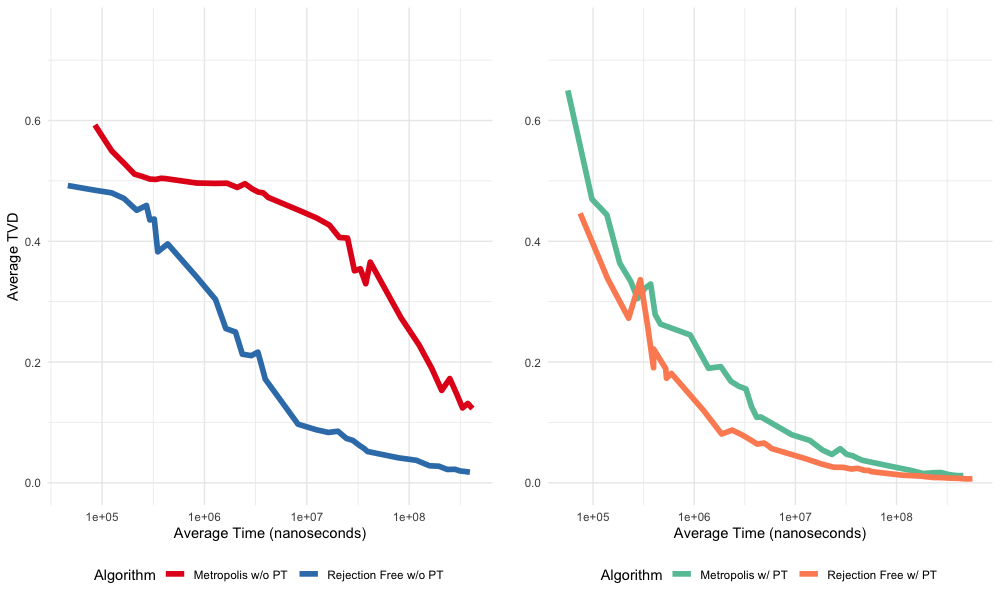
Figure 9: Average total variation distance TVD$(n)$ between sampled and actual distributions as a function of CPU time cost, for four scenarios: Metropolis versus Rejection-Free both without (left) and with (right) Parallel Tempering.

As a final check, we also calculated the effective sample size, similar to the first example. First, we generated 100 MCMC chains of $100,000$ iterations each, from all four algorithms. Then, we calculated the effective sample size for each chain, and normalized the results by either the number of iterations or the total CPU time for each algorithm. Table 3 shows the median of ESS per iteration and ESS per CPU second. It again illustrates that Rejection-Free can produce great speedups, increasing the ESS per CPU second by a factor of over 50 without Parallel Tempering, or a factor of 2 with Parallel Tempering.

	ESS per Iteration	ESS per CPU Second
Metropolis w/0 PT	0.0003	77.76
Rejection-Free w/o PT	0.0016	4,227
Metropolis w/ PT	0.0057	11,830
Rejection-Free w/ PT	0.0138	23,459

Table 3: Median of Normalized Effective Sample Sizes for four scenarios: Metropolis and Rejection-Free, both with and without Parallel Tempering

7.3 A Pseudo-Marginal MCMC Example

If the target density itself is not available analytically, but an unbiased estimate exists, then pseudo-marginal MCMC [1] can still be used to sample from the correct target distribution. We next apply the Rejection-Free method to a pseudo-marginal algorithm to show that Rejection-Free can provide speedups in that case, too.

In the previous example of the $4\times 4$ Ising model, the target probability distributions were defined as

$$\Pi(S)\ \propto\ \exp\{-\frac{E(S)}{T}\}\,.$$

We now pretend that this target density is not available, and we only have access to an unbiased estimator given by

$$\Pi_{0}(S)\ \propto\ \Pi(S)\times A\ =\ \exp\{\frac{E(S)}{T}\}\times A\,,$$

where $A\sim\textrm{Gamma}(\alpha=10,\beta=10)$ is a random variable (which is sampled independently every time as we try to compute the target distribution). Note that ${\bf E}(A)=10/10=1$, so ${\bf E}[\Pi_{0}(S)]=\Pi(S)$, and the estimator is unbiased (though $A$ has variance $10/10^{2}=1/10>0$).

Using this unbiased estimate of the target distribution as for pseudo-marginal MCMC, we again investigated the convergence of samples produced by the same four scenarios: Metropolis and Rejection-Free, both with and without Parallel Tempering. Figure 10 shows the average total variation distance TVD$(n)$ between the sampled and the actual magnetization distributions, for 100 chains, as a function of the iteration $n$, keeping all the other settings the same as before. This figure is quite similar to Figure 8, again showing that with or without Parallel Tempering, the use of Rejection-Free provides significant speedup, even in the pseudo-marginal case.

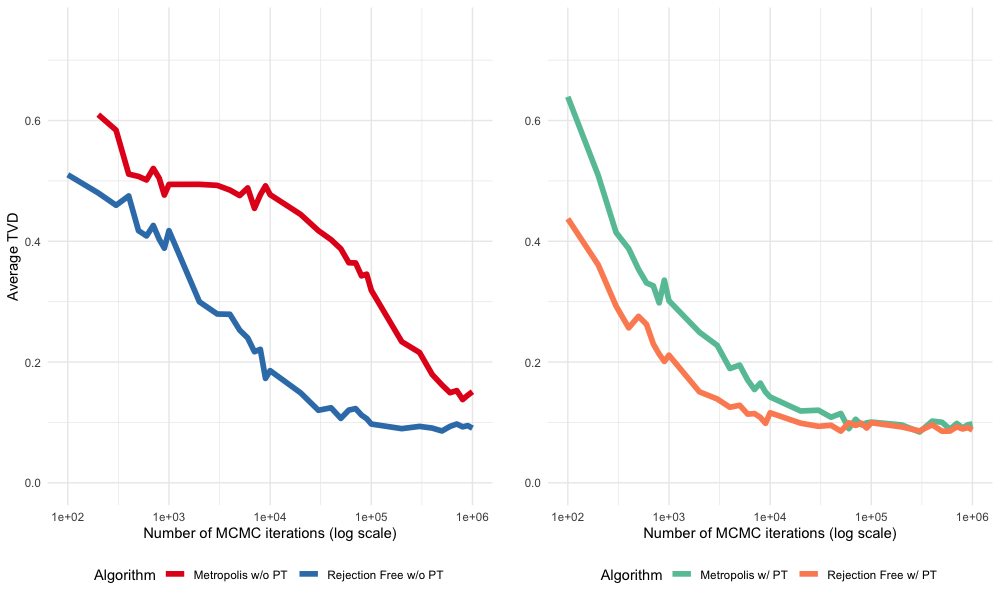
Figure 10: Average of total variation distance between sampled and actual distributions as a function of number of iterations for probability with noise Gamma(10, 10) in four scenarios: Metropolis versus Rejection-Free without Parallel Tempering (left) and with Parallel Tempering (right)

8 Summary

This paper has considered the use of parallelised computer hardware to run rejection-free versions of the Metropolis algorithm. We showed that the Uniform Selection Algorithm might fail to converge to the correct distribution or even visit the maximal value. However, the Jump Chain with appropriate weightings can provide consistent estimates of expected values in an efficient rejection-free manner. Care must be taken when alternating between multiple rejection-free chains, or when using rejection-free chains for parallel tempering, but appropriate adjustments allow for valid samplers in those cases as well. Simulations of our methods on several examples illustrate the significant speedups that result from using the Rejection-Free method to obtain more efficient samples.

9 Appendix: Proof of Proposition 1

Lemma 15.

For the Uniform Selection chain of Figure 6, let $s(x)={\bf P}($hit 4 before 0$\,|\,X_{0}=x)$. Then $s(0)=0$, $s(1)=3/7$, $s(2)=4/7$, $s(3)=13/21$, and $s(4)=1$.

Proof.

Clearly $s(0)=0$ and $s(4)=1$. Also, by conditioning on the first step, for $1\leq x\leq 3$ we have $s(x)=p_{x,x-1}\,s(x-1)+p_{x,x+1}\,s(x+1)$. In particular, $s(1)=(1/4)s(0)+(3/4)s(2)=(3/4)s(2)$, and $s(2)=(1/4)s(1)+(3/4)s(3)$, and $s(3)=(8/9)s(2)+(1/9)s(4)=(8/9)s(2)+(1/9)$. We solve these equations using algebra. Substituting the first equation into the second, $s(2)=(1/4)(3/4)s(2)+(3/4)s(3)$, so $(13/16)s(2)=(3/4)s(3)$, so $s(3)=(13/16)(4/3)s(2)=(13/12)s(2)$. Then the third equation gives $(13/12)s(2)=(8/9)s(2)+(1/9)$, so $(7/36)s(2)=(1/9)$, so $s(2)=(1/9)(36/7)=4/7$. Then $s(1)=(3/4)s(2)=(3/4)(4/7)=3/7$, and $s(3)=(8/9)s(2)+(1/9)=(8/9)(4/7)+(1/9)=13/21$, as claimed. ∎

Lemma 16.

Suppose the Uniform Selection chain for Example 2 begins at state $x=4a$ for some positive integer $a$. Let $C$ be the event that the chain hits $4(a+1)$ before hitting $4(a-1)$. Then $q:={\bf P}(C)=9/17>1/2$.

Proof.

By conditioning on the first step, we have that

$$q\ =\ {\bf P}(C\,|\,X_{0}=4a)\qquad\qquad\qquad\qquad\qquad\qquad\qquad\qquad\qquad\qquad\qquad\qquad\qquad$$

$$\ =\ {\bf P}(X_{1}=4a+1)\ {\bf P}(C\,|\,X_{0}=4a+1)+{\bf P}(X_{1}=4a-1)\ {\bf P}(C\,|\,X_{0}=4a-1)$$

$$\ =\ (1/2)\ {\bf P}(C\,|\,X_{0}=4a+1)+(1/2)\ {\bf P}(C\,|\,X_{0}=4a-1)\,.$$

But from $4a+1$, by Lemma 15, we either reach $4a+4$ before returning to $4a$ (and “win”) with probability 3/7, or we first return to $4a$ (and “start over”) with probability 4/7. Similarly, from $4a-1$, we either return to $4a$ (and “start over”) with probability 13/21, or we reach $4a-4$ before returning to $4a$ (and “lose”) with probability 8/21. Hence,

$$q\ =\ (1/2)\,[(3/7)+(4/7)q]+(1/2)\,[(13/21)q+0]\,.$$

That is, $q=(3/14)+(2/7)q+(13/42)q=(3/14)+(25/42)q$. Hence, $q=(3/14)\bigm{/}(17/42)=9/17>1/2$. ∎

We then have:

Corollary 17.

Suppose the Uniform Selection chain for Example 2 begins at state $4a\geq 8$ for some positive integer $a\geq 2$. Then the probability it will ever reach the state 4 is $(8/9)^{a-1}<1$.

Proof.

Consider a sub-chain $\{\tilde{X}_{n}\}$ of $\{X_{n}\}$ which just records new multiples of 4. That is, if the original chain is at the state $4b$, then the new chain is at $b$. Then, we wait until the original reaches either $4(b-1)$ or $4(b+1)$ at which point the next state of the new chain is $b-1$ or $b+1$ respectively. Then Lemma 16 says that this new chain is performing simple random walk on the positive integers, with up-probability 9/17 and down-probability 8/17. Then it follows from the Gambler’s Ruin formula (e.g. [20, equation 7.2.7]) that, starting from state $a$, the probability that the new chain will ever reach the state 1 is equal to $[(8/17)/(9/17)]^{a-1}=(8/9)^{a-1}<1$, as claimed. ∎

Since the chain starting at $4a$ for $a\geq 2$ cannot reach state 3 without first reaching state 4, Proposition 1 follows immediately from Corollary 17.

If we instead cut off the example at the state $4L$, then the Gambler’s Ruin formula (e.g. [20, equation 7.2.2]) says that from the state $4(L-1)$, the probability of reaching the state 4 before returning to the state $4L$ is $[(9/8)^{1}-1]\bigm{/}[(9/8)^{L-2}-1]<(8/9)^{L-1}$ (since $[A-1]\bigm{/}[B-1]<A/B$ whenever $1<A<B$), so the expected number of attempts to reach state 4 from state $4L$ is more than $(9/8)^{L-1}$.

Acknowledgements. This work was supported by research grants from Fujitsu Laboratories Ltd. We thank the editor and referees for very helpful comments which have greatly improved the manuscript.

References

- [1] C. Andrieu and G.O. Roberts (2009), The pseudo-marginal approach for efficient Monte Carlo computations. Ann. Stat. 37(2), 697–725.
- [2] A.B. Bortz, M.H. Kalos, and J.L. Lebowitz (1975), A New Algorithm for Monte Carlo Simulation of Ising Spin Systems. J. Comp. Phys. 17, 10–18.
- [3] S. Brooks, A. Gelman, G.L. Jones, and X.-L. Meng, eds. (2011), Handbook of Markov chain Monte Carlo. Chapman & Hall / CRC Press.
- [4] G. Deligiannidis and A. Lee (2018), Which ergodic averages have finite asymptotic variance? Ann. Appl. Prob. 28(4), 2309–2334.
- [5] R. Douc and C.P. Robert (2011), A vanilla Rao-Blackwellization of Metropolis-Hastings algorithms. Ann. Stat. 39, 261–277.
- [6] A. Doucet, M.K. Pitt, G. Deligiannidis, and R. Kohn (2015), Efficient implementation of Markov chain Monte Carlo when using an unbiased likelihood estimator. Biometrika 102(2), 295–313.
- [7] R. Durrett (1999), Essentials of stochastic processes. Springer, New York.
- [8] National Center for Education Statistics (2002), Education Longitudinal Study of 2002. Available at: https://nces.ed.gov/surveys/els2002/
- [9] C.J. Geyer (1991), Markov chain Monte Carlo maximum likelihood. In Computing Science and Statistics, Proceedings of the 23rd Symposium on the Interface, American Statistical Association, New York, 156–163.
- [10] W.K. Hastings (1970), Monte Carlo sampling methods using Markov chains and their applications. Biometrika 57, 97–109.
- [11] G. Iliopoulos and S. Malefaki (2013), Variance reduction of estimators arising from Metropolis-Hastings algorithms. Stat. Comput. 23, 577–587.
- [12] G. Kornissa, M.A. Novotnya, and P.A. Rikvoldab (1999), Parallelization of a Dynamic Monte Carlo Algorithm: A Partially Rejection-Free Conservative Approach. J. Comp. Phys. 153(2), 488–508.
- [13] B.D. Lubachevsky (1988), Efficient Parallel Simulations of Dynamic Ising Spin Systems. J. Comp. Phys. 75(1), 103–122.
- [14] S. Malefaki and G. Iliopoulos (2008), On convergence of properly weighted samples to the target distribution. J. Stat. Plan. Inference 138, 1210–1225.
- [15] N. Metropolis, A. Rosenbluth, M. Rosenbluth, A. Teller, and E. Teller (1953), Equations of state calculations by fast computing machines. J. Chem. Phys. 21, 1087–1091.
- [16] S.P. Meyn and R.L. Tweedie (1993), Markov chains and stochastic stability. Springer-Verlag, London. Available at: http://probability.ca/MT/
- [17] G.O. Roberts, A. Gelman, and W.R. Gilks (1997), Weak convergence and optimal scaling of random walk Metropolis algorithms. Ann. Appl. Prob. 7, 110–120.
- [18] G.O. Roberts and J.S. Rosenthal (2001), Optimal scaling for various Metropolis-Hastings algorithms. Stat. Sci. 16, 351–367.
- [19] G.O. Roberts and J.S. Rosenthal (2014), Minimising MCMC Variance via Diffusion Limits, with an Application to Simulated Tempering. Ann. Appl. Prob. 24, 131–149.
- [20] J.S. Rosenthal (2006), A first look at rigorous probability theory, 2nd ed. World Scientific Publishing, Singapore.
- [21] J.S. Rosenthal (2019), A first look at stochastic processes. World Scientific Publishing, Singapore.
- [22] R.H. Swendsen and J.S. Wang (1986), Replica Monte Carlo simulation of spin glasses. Phys. Rev. Lett. 57, 2607–2609.