Multi-material Topology Optimization of Lattice Structures using Geometry Projection

Abstract

This work presents a computational method for the design of architected truss lattice materials where each strut can be made of one of a set of available materials. We design the lattices to extremize effective properties. As customary in topology optimization, we design a periodic unit cell of the lattice and obtain the effective properties via numerical homogenization. Each bar is represented as a cylindrical offset surface of a medial axis parameterized by the positions of the endpoints of the medial axis. These parameters are smoothly mapped onto a continuous density field for the primal and sensitivity analysis via the geometry projection method. A size variable per material is ascribed to each bar and penalized as in density-based topology optimization to facilitate the entire removal of bars from the design. During the optimization, we allow bars to be made of a mixture of the available materials. However, to ensure each bar is either exclusively made of one material or removed altogether from the optimal design, we impose optimization constraints that ensure each size variable is 0 or 1, and that at most one material size variable is 1. The proposed material interpolation scheme readily accommodates any number of materials. To obtain lattices with desired material symmetries, we design only a reference region of the unit cell and reflect its geometry projection with respect to the appropriate planes of symmetry. Also, to ensure bars remain whole upon reflection inside the unit cell or with respect to the periodic boundaries, we impose a no-cut constraint on the bars. We demonstrate the efficacy of our method via numerical examples of bulk and shear moduli maximization and Poisson’s ratio minimization for two- and three-material lattices with cubic symmetry.

1 Introduction

Topology optimization techniques generate novel structural designs by optimizing the material layout within a prescribed design region. One of their applications is the design of architected materials with desired effective properties. This work focuses on the design of multi-material, periodic lattice structures via topology optimization. Open-cell lattice structures are generally easier to manufacture than most organic designs produced by topology optimization methods, as these may exhibit fully enclosed cavities. As all methods to design periodic structures, the goal of the proposed method is to design the unit cell, which we refer to in this work as the microstructure.

Methods to design microstructures were first introduced in ground-structure approaches. Sigmund presented an inverse homogenization method to design the microstructures by modeling the unit cell as a truss or thin frame structure [1, 2]. These methods benefit from efficient computation and naturally enforce a uniform cross-sectional area for the struts that simplifies their fabrication. However, they do not capture 3-dimensional stress states at strut intersections, and the optimal design may be suboptimal as it is a ‘subset’ of the ground structure.

The use of topology optimization of continua to design microstructures was first presented in density-based methods to design materials with extreme thermal expansion [3], and later employed in [4] to optimize the effective bulk modulus. This and similar approaches were also employed in [5, 6, 7, 8, 9, 10, 11]; cf. the recent review [12]. Compared to ground-structure approaches, these methods produce more efficient structures and are less dependent on the initial design. However, they can be more difficult to manufacture, specially closed-cell designs. Other topology optimization approaches to design microstructures include evolutionary approaches [13, 14, 15, 16] and level-set methods [17, 18, 19, 20]. Some methods concurrently design the topology of the micro and macrostructures [21, 22, 23, 24, 25, 26, 27, 28, 29]. This work, however, focuses only on the design of the microstructure. The multi-material topology optimization of microstructures was first demonstrated in the aforementioned works [3] and [4]. Other interpolation schemes (i.e., [30, 31]) have also been used to design multi-phase materials with extreme thermal conductivity [32, 33]. The reader is referred to [34] for a more detailed description of these approaches.

Although there exist multi-material additive manufacturing methods, the organic designs produced by the preceding methods are not necessarily easy to manufacture. They may possess closed cavities that require supports which are difficult to remove. Therefore, multi-material lattices made of struts may simplify their manufacturing. The geometry projection method [35, 36, 37] can be employed to design structures exclusively made of geometric components, whereby an analytic parameterization of the geometry is smoothly mapped onto a density field over a fixed finite element grid. By assigning a size variable to each geometric component that is penalized in the spirit of density-based methods, the geometry projection enables the entire removal of a component from the design. A similar family of methods to design structures made of discrete geometric components is the method of moving morphable components [38], in which geometric components and their union are represented using level set functions. Unlike the geometry projection method, this method does not employ penalized size variables for the components and therefore can only remove components by engulfing them inside other components or by making their size small enough that they do not affect the analysis.

The geometry projection method was employed in [39] in conjunction with an adaptation of the multi-material interpolation scheme of [3] to design two-material, 3-dimensional lattice structures. Its effectiveness is demonstrated via the design of two-material lattices for maximal bulk modulus and for minimal Poisson’s ratio. While this interpolation scheme is very effective, extending its application to more than two materials is not straightforward and requires changes to the material interpolation formulation, as noted in [40]. In the context of topology optimization with discrete geometric components using geometry projection, a new interpolation scheme was presented in [34] to accommodate the design of multi-material structures. A size variable per material is ascribed to each geometric component. This interpolation is an adaptation of the discrete material optimization (DMO) method [40]. However, unlike DMO, this method employs optimization constraints to ensure these size variables are 0 or 1, and to guarantee that each component has at most one material with a size variable of 1. The moving morphable component method has been applied to the design of multi-material structures [41] with geometric components made of different materials; however, unlike all of the aforementioned multi-material methods, the choice of material for each component is fixed and therefore not part of the optimization.

This work focuses on the topology optimization of multi-material lattice structures using the geometry projection method. By employing the multi-material interpolation and optimization constraints introduced in [34], the proposed method can readily accommodate any number of materials. It employs inverse homogenization to design the unit cell for extremizing the effective properties of the macrostructure. To enforce desired symmetries in the lattice, the geometry projection of a reference region is reflected onto other regions with respect to the symmetry planes corresponding to the desired symmetry. To ensure bars remain whole upon reflection inside the unit cell or with respect to the periodic boundaries and thus facilitate fabrication, we impose a volume difference constraint on the bars. This work builds on the preliminary results presented in [42] for maximal bulk modulus design by adding a no-cut constraint to ensure that bars remain whole upon reflection, which results in significantly different designs. We demonstrate the efficacy of our method by designing two- and three-material lattices with maximal bulk modulus, maximal shear modulus and minimal Poisson’s ratio subject to a weight constraint.

The rest of the paper is organized as follows. Section 2 discusses the projection of bnto analysis grid and the aggregation function and multi-material interpolation scheme. In Section 3 we describe the homogenization method that we use to calculate effective properties of the macrostructure by considering a unit cell. In Section 4 we employ reflection matrices to enforce symmetries on the lattice. Section 5 presents a new constraint to enforce the bars to stay in the symmetry reference region. The optimization problem in described in Section 6. We present numerical examples to demonstrate our method in Section 7 , and we draw conclusions in Section 8.

2 Geometry Projection

We employ the geometry projection method to create a differentiable map between a high-level parametric description of geometry and a density field defined over a fixed design region. For the lattice design, we consider structures made of cylindrical bars of the same diameter. We model a bar $q$ of diameter $w$ as an offset surface of a line segment (the bar’s medial axis), resulting in a cylinder with semi-spherical ends. We parameterize this geometric representation with the positions of the endpoints of the medial axis, $\mathbf{x}_{q_{o}}$ and $\mathbf{x}_{q_{f}}$ (cf. Fig. 1(a)). We calculate the projected density for point $\mathbf{p}$ as the volume fraction of the intersection of a sample window $\mathbf{B}_{\mathbf{p}}^{r}:=\{\mathbf{x}|\;\|\mathbf{p}-\mathbf{x}\|\leq r\}$ and the solid structure $\omega$:

$$\rho(\mathbf{x},r):=\frac{|\mathbf{B}_{\mathbf{p}}^{r}\cap\omega|}{\mathbf{B}_{\mathbf{p}}^{r}}$$ (1)

(a) Bar geometry

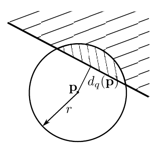
(b) Sample window

Figure 1: Geometry projection

This projected density is approximated as the volume fraction of the circular cap of height $r-\phi_{q}$ (cf. Fig. 1(b)), i.e.:

$$\rho_{q}(\phi_{q},r)=\left\{\begin{array}[]{ll}0&\mbox{if }\phi_{q}>r\\ \frac{1}{2}+\frac{\phi_{q}^{3}}{4r^{3}}-\frac{3\phi_{q}}{4r}&\mbox{if }-r\leq\phi_{q}\leq r\\ 1&\mbox{if }\phi_{q}<-r\\ \end{array}\right.$$ (2)

The signed distance $\phi_{q}(\mathbf{p})$ from $\mathbf{p}$ to bar $q$ is obtained from

$$\phi_{q}(d_{q},w):=d_{q}(\mathbf{x}_{q_{o}},\mathbf{x}_{q_{f}},\mathbf{p})-\frac{w}{2}$$ (3)

In the expression above, $d_{q}$ is the distance from $\mathbf{p}$ to the medial axis of bar $q$, given by:

$$d_{q}(\mathbf{x}_{q_{o}},\mathbf{x}_{q_{f}},\mathbf{p})=\left\{\begin{array}[]{ll}\|\mathbf{b}\|&\quad\mbox{if }\mathbf{a}\cdot\mathbf{b}\leq 0\\ \|\mathbf{g}\|&\quad\mbox{if }0<\mathbf{a}\cdot\mathbf{b}<\mathbf{a}\cdot\mathbf{a}\\ \|\mathbf{e}\|&\quad\mbox{if }\mathbf{a}\cdot\mathbf{b}>\mathbf{a}\cdot\mathbf{a}\\ \end{array}\right.$$ (4)

where

$$\mathbf{a}:=\mathbf{x}_{q_{f}}-\mathbf{x}_{q_{o}}\qquad\mathbf{b}:=\mathbf{p}-\mathbf{x}_{q_{o}}\qquad\mathbf{e}:=\mathbf{p}-\mathbf{x}_{q_{f}}\qquad\mathbf{g}:=\mathbf{P}_{\mathbf{a}}^{\perp}\mathbf{b}$$

and $\mathbf{P}_{a}^{\perp}=\mathbf{I}-(\mathbf{a}\otimes\mathbf{a})/\|\mathbf{a}\|^{2}$ is the perpendicular projection matrix on $\mathbf{a}$.

To calculate the projected density considering the contribution of multiple bars, a $p$-norm approximation of the maximum function is employed in [35, 36]. Unlike these works, in which all bars are made of the same isotropic material, [34] presented a new aggregation scheme to account for the intersection of bars made of different materials by defining an effective density for material $i$ at point $\mathbf{p}$, i.e.,

$$\rho_{eff}^{i}(\mathbf{z},\mathbf{p})=\frac{\sum_{q=1}^{N_{b}}\tilde{H}_{\epsilon}(-\phi_{q}(\mathbf{z},\mathbf{p}))\rho_{q}w_{i}^{q}(\mathbf{z})}{A+B}$$ (5)

where

$$A =\sum_{q=1}^{N_{b}}\left(\tilde{H}_{\epsilon}(-\phi_{q}(\mathbf{z},\mathbf{p}))\sum_{i=1}^{Nm}\alpha_{i}^{q}\right)$$ (6)

$$B =1-\underset{q}{KS}\left(\tilde{H}_{\epsilon}(-\phi_{q}(\mathbf{z},\mathbf{p}))\sum_{i=1}^{Nm}\alpha_{i}^{q}\right)$$ (7)

$$\underset{i}{KS}(\mathbf{x}) :=\frac{1}{k}\ln\left(\sum_{i}e^{kx_{i}}\right)$$ (8)

In the above expressions $N_{b}$ denotes the number of bars and $N_{m}$ the number of available materials; the term $A$ is an approximation of the number of solid bars containing $\mathbf{p}$, and the term $B$ equals unity to avoid a division by zero if point $\mathbf{p}$ lies in the void region; $KS$ is the Kreisselmeier-Steinhauser function, which smoothly approximates the maximum; and $\tilde{H}_{\epsilon}$ is a smooth relaxation of the Heaviside given by

$$\tilde{H}_{\epsilon}(x)=\left\{\begin{array}[]{ll}0&\quad\mbox{if }x<-\epsilon\\ \left[\frac{1}{2}+\frac{x}{2\epsilon}+\frac{1}{2\pi}\sin(\frac{\pi x}{\epsilon})\right]^{p}&\quad\mbox{if }-\epsilon\leq x\leq\epsilon\\ 1&\quad\mbox{if }x>\epsilon\end{array}\right.$$ (9)

with the parameter $p$ indicating the sharpness of the approximation. The weight fractions $w_{i}^{q}$ are defined in a the spirit of the DMO method, but defined using the size variables instead of the element densities as:

$$w_{i}^{q}=(\alpha_{i}^{q})\prod_{j=1}^{N_{m}}(1-(\alpha^{q}_{j\neq i}))$$ (10)

In the geometry projection method, as in density-based topology optimization techniques (and some level set optimization techniques), we employ an ersatz material to analyze the structure using a fixed mesh, whereby the effective elastic tensor at $\mathbf{p}$ is computed as:

$$\mathbb{C}(\mathbf{z},\mathbf{p})=\mathbb{C}_{min}+\sum_{i=1}^{N_{m}}\left(\mathbb{C}_{i}-\mathbb{C}_{min}\right)\,\rho_{eff}^{i}(\mathbf{z},\mathbf{p})$$ (11)

In this expression, $\mathbb{C}_{min}$ is the elasticity tensor of a weak isotropic material to preclude an ill-posed analysis, and $\mathbb{C}_{i}$ is the elasticity tensor for material $i$. The main difference between this material interpolation and the one used by multi-material density-based methods is that the material interpolation is uncoupled from the penalization (to ensure 0-1 size variables in the optimal design) and the mutual material exclusion (which ensures each bar is made of at most one material). We achieve this by imposing separate constraints in the optimization, which facilitates accommodating any number of materials.

3 Homogenization

We approximate the effective properties of the lattice by using homogenization (cf., [43, 44, 45, 46]). The components of the effective elastic tensor $\mathbb{C}^{H}$ are given by

$$C_{ijkl}^{H}=\frac{1}{|Y|}\int_{Y}C_{pqrs}(\epsilon_{pq}^{0(ij)}-\epsilon_{pq}^{*(ij)})(\epsilon_{rs}^{0(kl)}-\epsilon_{rd}^{*(kl)})~{}\mathop{}\!\mathrm{d}y$$ (12)

with $\bm{\epsilon}^{0(kl)}=\mathbf{e}_{k}\otimes\mathbf{e}_{l}$ corresponding to six unit strains applied on the unit cell, $Y$ denoting the domain of the unit cell, $C_{pqrs}$ indicating the components of the elasticity tensor of Eq. 11, and

$$\epsilon_{pq}^{*(kl)}=\frac{1}{2}\left(\frac{\partial\chi_{p}^{(kl)}}{\partial y_{q}}+\frac{\partial\chi_{q}^{(kl)}}{\partial y_{p}}\right)$$ (13)

The fields $\bm{\chi}^{(kl)}\in\mathcal{U}_{adm}$ are the solutions to the six problems

$$\int_{Y}C_{ijpq}\frac{\partial\chi_{p}^{(kl)}}{\partial y_{q}}\frac{\partial v_{i}}{\partial y_{j}}~{}\mathop{}\!\mathrm{d}y=\int_{Y}C_{ijkl}\frac{\partial v_{i}}{\partial y_{j}}~{}\mathop{}\!\mathrm{d}y,\forall\mathbf{v}\in\mathcal{U}_{adm}$$ (14)

with $\mathbf{v}$ denoting the test function and $\mathcal{U}_{adm}:=\{\mathbf{u}|\mathbf{u}\in H^{1}(Y),\mathbf{u}\text{ is }Y\text{--periodic}\}$ being the set of admissible solutions.

4 Symmetry

We impose symmetry with respect to an arbitrary number of planes on the unit cell to obtain desired material symmetries on the lattice. The intersection of these planes defines a number of similar regions, among which we choose one as the reference region, wherein we define the bars. To compute the projected density at a point in any of the other regions, we reflect the point with respect to the appropriate symmetry planes so that the reflected point lies on the reference region, and then we perform the geometry projection as usual. This strategy is employed in [34] and is similar to the one introduced in [39]. To perform the reflection with respect to the appropriate symmetry planes, we multiply all the corresponding reflection matrices (we assume all symmetry planes pass through the origin of the unit cell coordinate system). The reflected point is obtained as

$$\hat{\mathbf{p}}:=\prod_{s=1}^{N_{s}}\mathbf{R}_{s}\mathbf{p}\\$$ (15)

with $N_{s}$ denoting the number of symmetry planes and $\mathbf{R}_{s}$ being the reflection matrix corresponding to symmetry plane $s$.

5 No-Cut Constraint

A significant difference of the proposed method with the preliminary results of [42] is that here we introduce a constraint in the optimization to ensure components remain whole in the design space, that is, that lattice bars are not cut upon reflection or across boundaries, which would make fabrication more difficult. A mechanism to achieve this is introduced in [39] by imposing constraints on the positions of the endpoints of the bar’s medial axes so that they entirely lie within the reference region; in the case of cubic symmetry, for instance, this amounts to lower and upper bounds on the endpoint positions (which render orthotropic symmetry) plus four additional constraints per bar to restrict the positions to the reference tetrahedral region.

Here, we follow a simpler but equally effective approach, whereby we introduce a constraint on the difference between the volume of the bars in the reference region computed using the geometric parameters, and the volume that would be computed using the geometry projection. If these two volumes are different, it means a portion of the bar is lying outside of the reference region and the bar is cut. Therefore, if we impose a constraint that this difference cannot be larger than a small value, we consequently force bars to be wholly placed within the reference region. To account for multiple bars, we place the constraint on the maximum volume difference violation of all bars, which we smoothly approximate using a lower-bound KS function:

$$g_{n}(\mathbf{z}):=\underset{q}{LKS}(V_{geom}^{q}-V_{num}^{q})\leq\varepsilon_{n}$$ (16)

with

$$\underset{i}{LKS}(\mathbf{x}):=\frac{1}{k}\ln\left(\frac{1}{n}\sum_{i}e^{kx_{i}}\right),\,\mathbf{x}\in\mathbb{R}^{n}$$ (17)

where $V_{geom}^{q}$ is the volume of bar $q$ calculated using its geometric parameters (i.e., endpoint locations and width), and $V_{num}$ is the sum of projected densities for bar $q$ inside the symmetry reference region. The advantages of this approach are that it does not require formulating different placement constraints on the points for different types of material symmetries, and it renders a single optimization constraint regardless of the number of bars and of symmetry planes. We use the lower-bound KS function instead of the KS function of Eq. 8 because it approximates the maximum from below and therefore the approximation does not exceed the desired maximum value of zero. Also, we do not need to use adaptive constraint scaling strategies to compensate for the approximation error similar to those used in, e.g., stress-based topology optimization (cf., [47]) because the constraint limit is zero and we are approximating from below.

6 Optimization and Computer Implementation

We consider three problems in this work: maximization of the effective bulk modulus, maximization of the effective shear modulus and minimization of the effective Poisson’s ratio of the lattice structure, all subject to a material resource constraint. This constraint is imposed on the weight fraction, which considers the physical densities of the materials, as opposed to the more prevalent volume fraction constraint. A weight fraction constraint is more meaningful for multi-material design problems than specifying arbitrary volume fraction limits for each material.

We also impose a discreteness constraint to ensure all size variables $\alpha_{q}^{i}$ for bar $q$ and material $i$ attain a value of either 0 or 1 in the optimal design. We also need to guarantee that each bar is made of at most one material. In other words, the size variable corresponding to that material should equal 1 and all other size variables should be 0; or all size variables should equal 0, signifying the bar is entirely removed from the design. We employ the discreteness and mutual-material exclusion constraints introduced in [34], which we describe in the sequel.

6.1 Discreteness Constraint

To facilitate the lattice fabrication, we desire bars that are made of only one material. Therefore, the size variables have to be either 0 or 1 in the optimal design. Thus we need a penalization scheme to make intermediate values of the size variables disadvantageous. We achieve this by imposing the equality constraint

$$g_{d}(\mathbf{z}):=4\underset{i,q}{LKS}(\bm{\alpha}^{T}(\mathbf{1}-\bm{\alpha}))=0$$ (18)

with $LKS(\mathbf{x})$ being the function defined in Eq. 17, and $\bm{\alpha}=[\bm{\alpha}_{1}^{T}\;\bm{\alpha}_{2}^{T}\ldots\bm{\alpha}_{N_{b}}^{T}]^{T}$ denoting the vector of all size variables in the lattice, where $\bm{\alpha}_{q}$ is the $N_{m}$-vector of size variables for bar $q$ and $N_{m}$ is the number of materials. Since it is easier to enforce inequality constraints with the optimizer we employ in this work, we replace the constraint of Eq. 18 with the inequality constraint

$$g_{d}(\mathbf{z})\leq\varepsilon_{d}\ll 1$$ (19)

This explicit penalization of the size variables is similar to approaches employed in some density-based topology optimization techniques (e.g., [48]) to penalize intermediate density values. In those approaches, however, the explicit penalization is added as a penalty term to the objective function. As noted in [49], the challenge with this approach is to choose an adequate weighting factor for the penalty term that ensures good convergence. In our case, however, the explicit penalization is incorporated as an optimization constraint. Moreover, the fact that we are using the $LKS$ smooth maximum approximation allows us to choose a value for $\varepsilon$ that works well regardless of the number of bars.

Additionally, to prevent the design from quickly selecting a material for a bar that results in a poor local minimum, we employ a continuation strategy. We gradually decrease a relatively large initial value $\varepsilon_{d}^{(0)}$ by a step $\Delta\varepsilon_{d}$. This decrease is performed only after the relative change in the objective function in consecutive iterations is less than a specified value $\Delta f^{*}$, i.e.:

$$\text{If }\Delta f^{(I+1)}\leq\Delta f^{*}\text{ then }\varepsilon_{d}^{(I+1)}\leftarrow\max(\varepsilon_{d}^{(I)}-\Delta\varepsilon_{d},\varepsilon_{d}^{*})$$ (20)

where $\varepsilon_{d}^{*}$ is the final constraint limit and $\Delta f^{(I+1)}:=(|f^{(I+1)}-f^{(I)}|)/f^{(I)}$ the relative change in the objective function at iteration $I+1$. As observed in the numerical experiments in this work and in [42], this continuation strategy is effective in preventing premature convergence to poor local minima and renders good convergence.

6.2 Mutual Material Exclusion Constraint

To ensure each bar is either void or exclusively made of a single material, we impose the constraint

$$g_{m}(\mathbf{z}):=\underset{q}{LKS}\left(\sum_{i=1}^{N_{m}}\alpha_{i}^{q}\right)-1\leq 0$$ (21)

We use the same continuation strategy of Section 6.1 for this constraint. As with the case of the discreteness constraint described in the preceding section, the mutual material exclusion constraint is an explicit penalization enforced through a constraint in the optimization, as opposed to the implicit penalization employed by the DMO method.

6.3 Optimization Problem

In this work, we only consider effective lattices with cubic symmetry. However, as demonstrated in [42] for the case of bulk modulus maximization, the application to orthotropic materials is straightforward. The effective bulk ($K$) and shear ($G$) moduli are calculated as:

$$K(\mathbf{z})=\frac{1}{9}(C_{1111}+C_{1122}+C_{1133}+C_{2211}+C_{2222}+C_{2233}+C_{3311}+C_{3322}+C_{3333})\\$$ (22)

$$G(\mathbf{z})=\frac{1}{3}(C_{2323}+C_{1313}+C_{1212})\\$$ (23)

The Poisson’s ratio is given by:

$$\nu(\mathbf{z})=\frac{C_{1122}}{2(C_{1122}+C_{1212})}\\$$ (24)

The optimization problem is given by:

$$\underset{\mathbf{z}}{\min}f(\mathbf{z})$$ (25)

subject to

$$w_{f}:=\frac{1}{|\Omega|\gamma_{max}}\sum_{i=1}^{N_{m}}\gamma_{i}\int_{\Omega}\rho_{eff}^{i}(\mathbf{z},\mathbf{p})\mathop{}\!\mathrm{d}v\leq w_{f}^{*}$$ (26)

$$\mathsf{a}(\mathbf{u}^{(kl)}(\mathbf{z}),\mathbf{v})=\mathsf{l}(\mathbf{v},\bm{\epsilon}^{0(kl)}),\,\forall\mathbf{v}\in\mathcal{U}_{0},\mathbf{u}^{(kl)}\in\mathcal{U}$$ (27)

$$g_{d}(\mathbf{z})\leq\varepsilon_{d}^{(I)}$$ (28)

$$g_{m}(\mathbf{z})\leq\varepsilon_{m}^{(I)}$$ (29)

$$g_{n}(\mathbf{z})\leq\varepsilon_{n}$$ (30)

$$\mathbf{x}_{q_{0}},\mathbf{x}_{q_{f}}\in\Omega$$ (31)

$$0.0\leq\alpha_{i}^{q}\leq 1.0$$ (32)

with $f(\mathbf{z})\equiv-K(\mathbf{z})$ for the bulk modulus maximization, $f(\mathbf{z})\equiv-G(\mathbf{z})$ for the shear modulus maximization, and $f(\mathbf{z})\equiv\nu(\mathbf{z})$ for the Poisson’s ratio minimization. In addition to the foregoing constraints, and as is customary for this problem (cf. [1]), for the Poisson’s ratio minimization we also impose a lower limit on the effective bulk modulus, $K(\mathbf{z})\leq K_{min}$ to avoid removal of all the material. In the expressions above, $w_{f}$ is the weight fraction, $\gamma_{i}$ the physical density for material $i$, and $\gamma_{max}$ is the largest physical density of all available materials, so that if the heaviest material occupies the entire unit cell, $w_{f}=1$. The domains $\Omega$ and $\omega\subseteq\Omega$ correspond to the region occupied by the design envelope and the design, respectively. The test functions are denoted by $\mathbf{v}$, and $\mathbf{u}^{(kl)}$ are the displacements corresponding to the six applied unit strains $\bm{\epsilon}^{0(kl)}$, $k,l=1,\cdots,3$. The admissible sets for trial and test functions are $\mathcal{U}:=\{\mathbf{u}|\mathbf{u}\in H^{1}(\Omega),\mathbf{u}\text{ is }Y\text{-periodic},\mathbf{u}(\mathbf{c})=\mathbf{0}\}$ and $\mathcal{U}_{0}:=\{\mathbf{v}|\mathbf{v}\in H^{1}(\Omega),\mathbf{v}|_{\Gamma}=\mathbf{0},\mathbf{v}(\mathbf{c})=\mathbf{0}\}$, respectively. We prevent rigid-body motions by imposing zero displacements at the center of the unit cell $\mathbf{c}$. The energy bilinear form $\mathsf{a}$ and the load linear form $\mathsf{l}$ in Eq. 27 are computed as:

$$\mathsf{a}(\mathbf{u},\mathbf{v}) :=\int_{\Omega}\nabla\mathbf{v}\cdot\mathbb{C}(\mathbf{z},\mathbf{p})\nabla\mathbf{u}\mathop{}\!\mathrm{d}v$$ (33)

$$\mathsf{l}(\mathbf{v},\bm{\epsilon}) :=\int_{\Omega}\nabla\mathbf{v}\cdot\mathbb{C}(\mathbf{z},\mathbf{p})\bm{\epsilon}\mathop{}\!\mathrm{d}v$$ (34)

For the design variables $\hat{z}$ to fall within the range $[0,1]$, we scale them as in our previous works [36, 37, 34], and at each optimization iteration $I$ we impose a move limit $m$ on each design variable as:

$$\max(0,\mathbf{z}^{(I-1)}-m)\leq\mathbf{z}^{(I)}\leq\min(1,\mathbf{z}^{(I-1)}+m)$$ (35)

6.4 Computer Implementation

A flowchart describing the proposed method is shown in Algorithm 1. Our code is implemented in C++ using the deal.II library [50, 51] as a backbone for the finite element solutions. We parallelize the assembly of the stiffness matrix, the computation of geometry projection, and the solution of the linear system of equations by employing the data structures provided by parallel linear algebra libraries. We employ an element-wise uniform effective density, which we compute at the element centroid $\mathbf{x}_{e}$. The geometry projection is computed using a window radius $r$ equal to $c$ times the radius of the sphere that circumscribes the element, i.e., $r=c\sqrt{3}h/2$, where $h$ is the element size. As the optimizer, we employ the parallel implementation of the method of moving asymptotes (MMA) of [52, 53], presented in [54]. We use the default MMA parameters presented in [53]. We stop the optimization when the relative change $\Delta f$ in compliance between consecutive iterations falls below a specified value $\Delta f^{*}$. The optimization parameter values we employed for all examples are listed in Table 1.

Algorithm 1 Multi-material Topology Optimization of Lattice Structures

1:$k\leftarrow 0$ $\triangleright$ Iteration counter

2:$\mathbf{z}^{(0)}\leftarrow\mathbf{z}_{0}$ $\triangleright$ Initial design

3:$f_{old}=-objtol$

4:repeat

5:    for $q=1,\ldots,N_{b}$ do

6:         for $e=1,\ldots,N_{el}$ do

7:             Compute signed distance $\phi_{q}$ to bar $q$ $\triangleright$ §2

8:             if element $e$ outside of the reference region then

9:                 Computed reflected element centroid $\hat{\mathbf{x}}_{e}$ $\triangleright$ Eq. (15)

10:             end if

11:             Compute projected density $\rho_{q}$ $\triangleright$ Eq. (3)

12:         end for

13:    end for

14:    for $k=1,\ldots,6$ do

15:         for $e=1,\ldots,N_{el}$ do

16:             Compute element stiffness matrix $\mathbf{K}_{e}^{k}$ using $\mathbb{C}(\mathbf{z},\mathbf{p})$ $\triangleright$ Eq. (11)

17:             Assemble $\mathbf{K}_{e}^{k}$ into global stiffness matrix $\mathbf{K}_{k}$

18:             Compute element force $\mathbf{f}_{e}^{k}$ contributions from applied unit strains $\triangleright$ Eq. (27)

19:             Assemble $\mathbf{f}_{e}^{k}$ into global force vectors $\mathbf{f}_{k}$

20:         end for

21:         Solve $\mathbf{K}_{k}(\mathbf{z})\mathbf{u}_{k}(\mathbf{z})=\mathbf{f}_{k}$ for $\mathbf{u}(\mathbf{z})$

22:    end for

23:    Compute $f(\mathbf{z})$, $\nabla f(\mathbf{z})$ $\triangleright$ Eq. (22) or Eq. (23) or Eq. (24)

24:    Compute $\mathbf{g}(\mathbf{z})$, $\nabla\mathbf{g}(\mathbf{z})$ $\triangleright$ $\mathbf{g}$ denotes vector of constraints

25:    Impose move limits and update $\mathbf{z}_{low}$ and $\mathbf{z}_{upp}$ $\triangleright$ Eq. (35)

26:    $\mathbf{z}^{(k+1)}\leftarrow\texttt{opt}(\mathbf{z}^{(k)},f,\nabla f,\mathbf{g},\nabla\mathbf{g},\mathbf{z}_{low},\mathbf{z}_{upp})$ $\triangleright$ Update design

27:    $k\leftarrow k+1$

28:    Compute relative change in objective $\Delta f=|(f-f_{old})/f_{old}|$

29:    $f_{old}\leftarrow f$

30:until $\Delta f\leq objtol$

Parameter	Value	Equation/Section
$\varepsilon_{d}^{0}$	1.0	19
$\varepsilon_{d}^{*}$	0.01	20
$\varepsilon_{m}^{0}$	0.3	§6.2
$\varepsilon_{m}^{*}$	0.01	§6.2
$\varepsilon_{n}$	$10^{-5}$	16
$K_{min}$	0.001	§6.3
$p$	2	9
$k$	25	8
$m$	0.1	35
$c$	1.0	§6.4

Table 1: Optimization parameters

7 Examples

We now present examples to illustrate the effectiveness of the proposed method. We employ hexahedral, trilinear elements to mesh the unit cell. We employ a system with six compute nodes with 24 Intel Haswell cores each, CPU speed of 2.59 GHz and 128 GB of memory per node to perform all the examples.

7.1 Maximal Bulk Modulus of Two- and Three-material Lattices with Cubic Symmetry

In this example, we maximize the bulk modulus for lattices with cubic symmetry and made of two and three materials. To enforce the cubic symmetry, we define nine symmetry planes, including the three orthogonal planes perpendicular to the faces that pass through the center of the unit cell, and the six planes that pass through the origin and two opposite edges that divide the cube into two equal partitions. The initial design consists of 10 bars with near-zero length (which resemble spheres) and width $w=0.1$, as shown in Fig. 2. All materials are homogeneous, isotropic, and linearly elastic, with Poisson’s ratio $\nu=0.3$. The unit cell is meshed with a regular grid of $64\times 64\times 64$ elements.

For the two-material designs, the available materials have Young’s moduli $E_{1}=10$ and $E_{2}=5$, and physical densities $\gamma_{1}=0.9$ and $\gamma_{2}=0.45$. We set the initial size variables corresponding to these two materials to $\alpha_{1}^{q}=\alpha_{2}^{q}=0.5$.

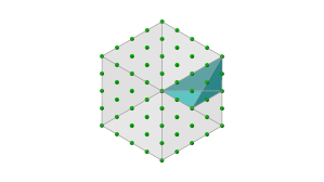
Figure 2: Initial design after reflection for cubic symmetry. Blue region indicates reference region.

The results of the optimization for different weight fraction limits are presented in Table  2. It is worth noting that small changes in the weight fraction limit produce completely different designs. This is expected, since this problem is known to have many local minima [55]. The overall trend is that the maximal bulk modulus increases as we increase the weight fraction limit as expected. We posit the exceptions to a strict monotonic behavior correspond to convergence to local minima. One possibility to obtain better minima would be to employ the tunneling method proposed in [56]; however, this is outside the scope of this paper.

An important difference between these results and those previously published in [42] is that the no-cut constraint is effective in rendering struts that do not have cuts that would be difficult to manufacture. The no-cut constraint also performs an important task, namely to prevent agglomerations of cut struts on a face of the unit cell to effectively produced a thin wall, which produces a closed-cell design (this situation was observed in [42]).

$K$	$w_{f}^{*}$	iso	side	$K$	$w_{f}^{*}$	iso	side
$0.06999$	$0.0444$			$0.13853$	$0.0778$
$0.08031$	$0.05$			$0.12034$	$0.0833$
$0.09229$	$0.0556$			$0.13908$	$0.0889$
$0.1171$	$0.0611$			$0.15736$	$0.0944$
$0.09543$	$0.0667$			$0.18651$	$0.1$
$0.12366$	$0.0722$			$0.17525$	$0.1056$

Table 2: Maximal bulk modulus designs for cubic two-material lattices and different weight fraction limits $w_{f}^{*}$. Red bars are made of material 1, blue bars are made of material 2, and bars that have been removed from the design (i.e., with $\alpha_{1}^{q},\alpha_{2}^{q}\approx 0$) are not shown.

In Fig. 3(a), we compare the effective bulk moduli for the designs of Table 2 to the Hashin-Shtrikman-Walpole bounds for three-phase materials (with one phase being void) [4]. As expected, all the bulk moduli for the optimal designs are below the bounds. We also note that the moduli are not close to the bounds. This is contrary to what has been shown for designs obtained using density-based topology optimization [4]. The reason for this is that the design representation is significantly more restrictive (i.e., a truss made of cylindrical struts of constant diameter) and we impose an additional geometric requirement (the no-cut constraint). Moreover, the lattice representation ensures an open-cell design (which we desire, as justified in Section 1); however, closed-cell designs are known to render higher bulk moduli [55].

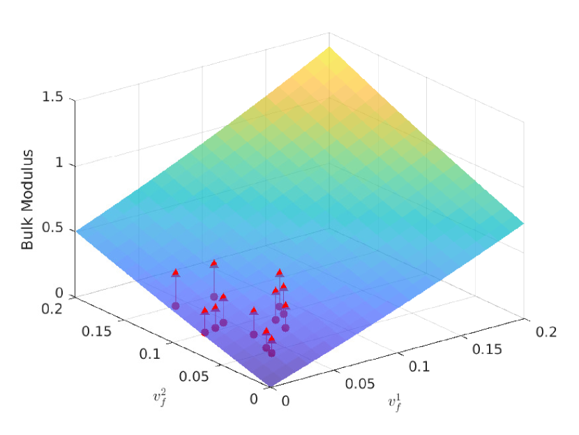
(a) Effective bulk modulus

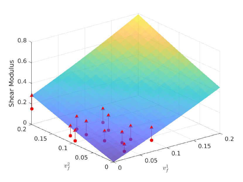
(b) Effective shear modulus

Figure 3: Comparison of effective moduli to HSW-bounds for the designs corresponding to Tables 2 and 4. Arrows point from the optimal design to the HSW-bound surface.

We now perform the optimization for this same problem by adding a third material with elastic modulus $E_{3}=7.5$ and physical density $\gamma_{3}=0.675$. The results for different weight fraction limits are shown in Table 3. An important note about these results is that the range of weight fraction limits that produces three-material designs is narrower than for two-material designs. This is expected, since above and below that range two-material designs (and eventually, single-material designs) are more weight-efficient.

$K$	$w_{f}^{*}$	iso	side
$0.09399$	$0.0667$
$0.12024$	$0.0889$
$0.16937$	$0.0944$
$0.15466$	$0.1$

Table 3: Maximal bulk modulus designs for cubic three-material lattices and different weight fraction limits $w_{f}^{*}$. Red, blue and green bars are made of materials 1, 2, and 3, respectively; and bars that have been removed from the design (i.e., with $\alpha_{1}^{q},\alpha_{2}^{q},\alpha_{3}^{q}\approx 0$) are not shown.

7.2 Two- and Three-material Lattices with Maximal Shear Modulus and Cubic Symmetry

In this section we present results for maximization of the effective shear modulus, both for two-material and three-material lattices. The material properties are the same as in the previous section. The results of the optimization of two-material lattices for different weight fraction limits are presented in Table  4. As before, we note that small changes in the weight fraction limit produce different designs. The overall trend is again that the maximal shear modulus increases as we increase the weight fraction limit as expected, however convergence to local minima likely prevents strict monotonicity. In Fig. 3(b), we compare the effective shear moduli for the designs of Table 4 to the Hashin-Shtrikman-Walpole bounds for three-phase materials. As with the bulk modulus, all the effective shear moduli for the optimal designs are below the bounds.

The results of the optimization for this same problem with three materials (with the same properties as before) are shown in Table 5. Once again, the range of weight fraction limits that produces three-material designs is narrower than for two-material designs.

$G$	$w_{f}^{*}$	iso	side	$G$	$w_{f}^{*}$	iso	side
$0.0242$	$0.0444$			$0.08252$	$0.0778$
$0.03494$	$0.05$			$0.05861$	$0.0833$
$0.05653$	$0.0556$			$0.0709$	$0.0889$
$0.0526$	$0.0611$			$0.08605$	$0.0944$
$0.05019$	$0.0667$			$0.15178$	$0.1$
$0.0563$	$0.0722$			$0.12434$	$0.1056$

Table 4: Maximal shear modulus designs for cubic two-material lattices and different weight fraction limits $w_{f}^{*}$. Red bars are made of material 1, blue bars are made of material 2, and bars that have been removed from the design (i.e., with $\alpha_{1}^{q},\alpha_{2}^{q}\approx 0$) are not shown.

$G$	$w_{f}^{*}$	iso	side
$0.04591$	$0.0556$
$0.03146$	$0.0722$
$0.08593$	$0.0944$
$0.1288$	$0.1056$

Table 5: Maximal shear modulus designs for cubic three-material lattices for different weight fraction limits $w_{f}^{*}$. Red, blue and green bars are made of materials 1, 2, and 3, respectively; and bars that have been removed from the design (i.e., with $\alpha_{1}^{q},\alpha_{2}^{q},\alpha_{3}^{q}\approx 0$) are not shown.

7.3 Two-material Lattices with Negative Poisson Ratio and Cubic Symmetry

Finally, we present results for the minimization of the effective Poisson’s ratio for two- and three-material cubic lattices. The material properties are the same as before. As detailed in Section 6, for this problem we add a constraint that ensures a minimum bulk modulus of $K_{min}$, cf. Table 1. The results for two-material lattices are shown in Table 6. For the weight fraction limits we employed, the resulting effective Poisson’s ratios are all negative, therefore the lattice is auxetic. In this case, the effective Poisson’s ratio monotonically decreases as we increase the weight fraction limit. We also present a three-material lattice design in Table 7. In this case, we could only find a narrow weight fraction limit range that would render a three-material design with negative Poisson’s ratio. We note, however, that the three-material design performs better than the two-material design for the same weight fraction limit shown in Table 6.

$\nu$	$w_{f}^{*}$	iso	side	$\nu$	$w_{f}^{*}$	iso	side
$-0.05721$	$0.0333$			$-0.63902$	$0.05$
$-0.11753$	$0.0389$			$-1.57259$	$0.0667$
$-0.204$	$0.0444$			$-3.81031$	$0.0722$

Table 6: Minimal Poisson’s ratio designs for cubic two-material lattices for different weight fraction limits $w_{f}^{*}$. Red bars are made of material 1, blue bars are made of material 2, and bars that have been removed from the design (i.e., with $\alpha_{1}^{q},\alpha_{2}^{q}\approx 0$) are not shown.

$\nu$	$w_{f}^{*}$	iso	side
$-0.42618$	$0.0389$

Table 7: Minimal Poisson’s ratio design for cubic three-material lattice. Red, blue and green bars are made of materials 1, 2, and 3, respectively; and bars that have been removed from the design (i.e., with $\alpha_{1}^{q},\alpha_{2}^{q},\alpha_{3}^{q}\approx 0$) are not shown.

8 Conclusions

This work presented a topology optimization method for the design of multi-material lattice structures using the geometry projection technique. The numerical examples demonstrate that the proposed method is effective in producing multi-material lattices for the maximization of effective bulk and shear moduli, and for the minimization of effective Poisson’s ratio. The proposed formulation effectively imposes any number of symmetry planes to obtain desired material symmetries; in the case of the numerical examples, cubic symmetry is imposed on all lattices. Moreover, the no-cut constraint is also effective in preventing struts from being cut by the unit cell boundaries or the symmetry planes that would make the manufacturing more difficult, and that may produce closed-cell structures. As expected, the designed lattices satisfy theoretical bounds on effective bulk and shear moduli, and are in fact away from these bounds since they are open-cell structures. The designs produced by the proposed method still pose some fabrication challenges, as some of the struts may have overlaps that are difficult to realize. Future work will be devoted to minimize strut overlaps, and to impose angle constraints on the struts to remove altogether the need for supports.

References

- [1] Ole Sigmund. Materials with prescribed constitutive parameters: an inverse homogenization problem. International Journal of Solids and Structures, 31(17):2313–2329, 1994.
- [2] Ole Sigmund. Tailoring materials with prescribed elastic properties. Mechanics of Materials, 20(4):351–368, 1995.
- [3] Ole Sigmund and Salvatore Torquato. Design of materials with extreme thermal expansion using a three-phase topology optimization method. Journal of the Mechanics and Physics of Solids, 45(6):1037–1067, 1997.
- [4] Leonid V Gibiansky and Ole Sigmund. Multiphase composites with extremal bulk modulus. Journal of the Mechanics and Physics of Solids, 48(3):461–498, 2000.
- [5] Ole Sigmund, S Torquato, and Ilhan A Aksay. On the design of 1–3 piezocomposites using topology optimization. Journal of materials research, 13(4):1038–1048, 1998.
- [6] MM Neves, H Rodrigues, and J Miranda Guedes. Optimal design of periodic linear elastic microstructures. Computers & Structures, 76(1-3):421–429, 2000.
- [7] Steven J Cox and David C Dobson. Band structure optimization of two-dimensional photonic crystals in h-polarization. Journal of Computational Physics, 158(2):214–224, 2000.
- [8] S Torquato, S Hyun, and A Donev. Multifunctional composites: optimizing microstructures for simultaneous transport of heat and electricity. Physical review letters, 89(26):266601, 2002.
- [9] James K Guest and Jean H Prévost. Optimizing multifunctional materials: design of microstructures for maximized stiffness and fluid permeability. International Journal of Solids and Structures, 43(22-23):7028–7047, 2006.
- [10] James K Guest and Jean H Prévost. Design of maximum permeability material structures. Computer Methods in Applied Mechanics and Engineering, 196(4-6):1006–1017, 2007.
- [11] Niek de Kruijf, Shiwei Zhou, Qing Li, and Yiu-Wing Mai. Topological design of structures and composite materials with multiobjectives. International Journal of Solids and Structures, 44(22-23):7092–7109, 2007.
- [12] Mikhail Osanov and James K Guest. Topology optimization for architected materials design. Annual Review of Materials Research, 46:211–233, 2016.
- [13] Xiaodong Huang and YM Xie. Optimal design of periodic structures using evolutionary topology optimization. Structural and Multidisciplinary Optimization, 36(6):597–606, 2008.
- [14] X Huang, A Radman, and YM Xie. Topological design of microstructures of cellular materials for maximum bulk or shear modulus. Computational Materials Science, 50(6):1861–1870, 2011.
- [15] X Huang, Yi Min Xie, Baohua Jia, Qing Li, and SW Zhou. Evolutionary topology optimization of periodic composites for extremal magnetic permeability and electrical permittivity. Structural and Multidisciplinary Optimization, 46(3):385–398, 2012.
- [16] A Radman, X Huang, and YM Xie. Topological optimization for the design of microstructures of isotropic cellular materials. Engineering optimization, 45(11):1331–1348, 2013.
- [17] VJ Challis, AP Roberts, and AH Wilkins. Design of three dimensional isotropic microstructures for maximized stiffness and conductivity. International Journal of Solids and Structures, 45(14-15):4130–4146, 2008.
- [18] Shiwei Zhou, Wei Li, Guangyong Sun, and Qing Li. A level-set procedure for the design of electromagnetic metamaterials. Optics express, 18(7):6693–6702, 2010.
- [19] Masaki Otomori, Takayuki Yamada, Kazuhiro Izui, Shinji Nishiwaki, and Nozomu Kogiso. Level set-based topology optimization for the design of light-trapping structures. IEEE Transactions on Magnetics, 50(2):729–732, 2014.
- [20] Renato Picelli, Raghavendra Sivapuram, Scott Townsend, and H Alicia Kim. Stress topology optimisation for architected material using the level set method. In World Congress of Structural and Multidisciplinary Optimisation, pages 1254–1269. Springer, 2017.
- [21] H Rodrigues, Jose M Guedes, and MP Bendsoe. Hierarchical optimization of material and structure. Structural and Multidisciplinary Optimization, 24(1):1–10, 2002.
- [22] JM Guedes, E Lubrano, HC Rodrigues, and S Turteltaub. Hierarchical optimization of material and structure for thermal transient problems. In IUTAM Symposium on Topological Design Optimization of Structures, Machines and Materials, pages 527–536. Springer, 2006.
- [23] PG Coelho, PR Fernandes, JM Guedes, and HC Rodrigues. A hierarchical model for concurrent material and topology optimisation of three-dimensional structures. Structural and Multidisciplinary Optimization, 35(2):107–115, 2008.
- [24] Ling Liu, Jun Yan, and Gengdong Cheng. Optimum structure with homogeneous optimum truss-like material. Computers & Structures, 86(13-14):1417–1425, 2008.
- [25] Bin Niu, Jun Yan, and Gengdong Cheng. Optimum structure with homogeneous optimum cellular material for maximum fundamental frequency. Structural and Multidisciplinary Optimization, 39(2):115, 2009.
- [26] Jun Yan, Geng-dong Cheng, and Ling Liu. A uniform optimum material based model for concurrent optimization of thermoelastic structures and materials. International Journal for Simulation and Multidisciplinary Design Optimization, 2(4):259–266, 2008.
- [27] Jiadong Deng, Jun Yan, and Gengdong Cheng. Multi-objective concurrent topology optimization of thermoelastic structures composed of homogeneous porous material. Structural and Multidisciplinary Optimization, 47(4):583–597, 2013.
- [28] X Huang, SW Zhou, YM Xie, and Q Li. Topology optimization of microstructures of cellular materials and composites for macrostructures. Computational Materials Science, 67:397–407, 2013.
- [29] X Yan, X Huang, Y Zha, and YM Xie. Concurrent topology optimization of structures and their composite microstructures. Computers & Structures, 133:103–110, 2014.
- [30] Martin P Bendsøe and Ole Sigmund. Material interpolation schemes in topology optimization. Archive of applied mechanics, 69(9-10):635–654, 1999.
- [31] Mathias Stolpe and Krister Svanberg. An alternative interpolation scheme for minimum compliance topology optimization. Structural and Multidisciplinary Optimization, 22(2):116–124, 2001.
- [32] Shiwei Zhou and Qing Li. The relation of constant mean curvature surfaces to multiphase composites with extremal thermal conductivity. Journal of Physics D: Applied Physics, 40(19):6083, 2007.
- [33] Shiwei Zhou and Qing Li. Computational design of multi-phase microstructural materials for extremal conductivity. Computational Materials Science, 43(3):549–564, 2008.
- [34] Hesaneh Kazemi, Ashkan Vaziri, and Julián A Norato. Topology optimization of structures made of discrete geometric components with different materials. Journal of Mechanical Design, 140(11):111401, 2018.
- [35] Bryan Bell, Julian Norato, and Daniel Tortorelli. A geometry projection method for continuum-based topology optimization of structures. In 12th AIAA Aviation Technology, Integration, and Operations (ATIO) Conference and 14th AIAA/ISSMO Multidisciplinary Analysis and Optimization Conference, page 5485, 2012.
- [36] JA Norato, BK Bell, and DA Tortorelli. A geometry projection method for continuum-based topology optimization with discrete elements. Computer Methods in Applied Mechanics and Engineering, 293:306–327, 2015.
- [37] Shanglong Zhang, Julián A Norato, Arun L Gain, and Naesung Lyu. A geometry projection method for the topology optimization of plate structures. Structural and Multidisciplinary Optimization, 54(5):1173–1190, 2016.
- [38] Xu Guo, Weisheng Zhang, and Wenliang Zhong. Doing topology optimization explicitly and geometrically—a new moving morphable components based framework. Journal of Applied Mechanics, 81(8):081009, 2014.
- [39] Seth Watts and Daniel A Tortorelli. A geometric projection method for designing three-dimensional open lattices with inverse homogenization. International Journal for Numerical Methods in Engineering, 2017.
- [40] Jan Stegmann and Erik Lund. Discrete material optimization of general composite shell structures. International Journal for Numerical Methods in Engineering, 62(14):2009–2027, 2005.
- [41] Weisheng Zhang, Junfu Song, Jianhua Zhou, Zongliang Du, Yichao Zhu, Zhi Sun, and Xu Guo. Topology optimization with multiple materials via moving morphable component (MMC) method. International Journal for Numerical Methods in Engineering.
- [42] Hesaneh Kazemi, Ashkan Vaziri, and Julián A Norato. Topology optimization of multi-material lattices for maximal bulk modulus (accepted). In ASME 2019 International Design Engineering Technical Conferences and Computers and Information in Engineering Conference. American Society of Mechanical Engineers, 2019.
- [43] JoséMiranda Guedes and Noboru Kikuchi. Preprocessing and postprocessing for materials based on the homogenization method with adaptive finite element methods. Computer methods in applied mechanics and engineering, 83(2):143–198, 1990.
- [44] Behrooz Hassani and Ernest Hinton. A review of homogenization and topology optimization i—homogenization theory for media with periodic structure. Computers & Structures, 69(6):707–717, 1998.
- [45] Behrooz Hassani and E Hinton. A review of homogenization and topology opimization ii—analytical and numerical solution of homogenization equations. Computers & structures, 69(6):719–738, 1998.
- [46] Behrooz Hassani and Ernest Hinton. A review of homogenization and topology optimization iii—topology optimization using optimality criteria. Computers & structures, 69(6):739–756, 1998.
- [47] Chau Le, Julian Norato, Tyler Bruns, Christopher Ha, and Daniel Tortorelli. Stress-based topology optimization for continua. Structural and Multidisciplinary Optimization, 41(4):605–620, 2010.
- [48] Thomas Borrvall and Joakim Petersson. Topology optimization using regularized intermediate density control. Computer Methods in Applied Mechanics and Engineering, 190(37-38):4911–4928, 2001.
- [49] Ole Sigmund and Kurt Maute. Topology optimization approaches. Structural and Multidisciplinary Optimization, 48(6):1031–1055, 2013.
- [50] W. Bangerth, R. Hartmann, and G. Kanschat. deal.II – a general purpose object oriented finite element library. ACM Trans. Math. Softw., 33(4):24/1–24/27, 2007.
- [51] G. Alzetta, D. Arndt, W. Bangerth, V. Boddu, B. Brands, D. Davydov, R. Gassmoeller, T. Heister, L. Heltai, K. Kormann, M. Kronbichler, M. Maier, J.-P. Pelteret, B. Turcksin, and D. Wells. The deal.II library, version 9.0. Journal of Numerical Mathematics, 26(4):173–183, 2018.
- [52] Krister Svanberg. A class of globally convergent optimization methods based on conservative convex separable approximations. SIAM Journal on Optimization, 12(2):555–573, 2002.
- [53] Krister Svanberg. MMA and GCMMA, versions september 2007. Optimization and Systems Theory, page 104, 2007.
- [54] Niels Aage, Erik Andreassen, Boyan S Lazarov, and Ole Sigmund. Giga-voxel computational morphogenesis for structural design. Nature, 550(7674):84, 2017.
- [55] Martin P Bendsøe and Ole Sigmund. Topology optimization: theory, methods and applications. 2003, 2013.
- [56] Shanglong Zhang and Julián A Norato. Finding better local optima in topology optimization via tunneling. In ASME 2018 International Design Engineering Technical Conferences and Computers and Information in Engineering Conference, pages V02BT03A014–V02BT03A014. American Society of Mechanical Engineers, 2018.