Sine-skewed toroidal distributions and their application in protein bioinformatics

Abstract

In the bioinformatics field, there has been a growing interest in modelling dihedral angles of amino acids by viewing them as data on the torus. This has motivated, over the past years, new proposals of distributions on the bivariate torus. The main drawback of most of these models is that the related densities are (pointwise) symmetric, despite the fact that the data usually present asymmetric patterns. This motivates the need to find a new way of constructing asymmetric toroidal distributions starting from a symmetric distribution. We tackle this problem in this paper by introducing the sine-skewed toroidal distributions. The general properties of the new models are derived. Based on the initial symmetric model, explicit expressions for the shape parameters are obtained, a simple algorithm for generating random numbers is provided, and asymptotic results for the maximum likelihood estimators are established. An important feature of our construction is that no normalizing constant needs to be calculated, leading to more flexible distributions without increasing the complexity of the models. The benefit of employing these new sine-skewed distributions is shown on the basis of protein data, where, in general, the new models outperform their symmetric antecedents.

Keywords: Directional Statistics; Flexible Modeling; Skewness; Structural Bioinformatics; Toroidal Data.

1 Introduction

Toroidal data are observations taking values on the unit torus, that is, the product of unit circles, the typical example being the torus in three dimensions formed by the product of two unit circles. This also explains the alternative terminology of circular-circular or bivariate circular data in $\mathbb{R}^{3}$. Toroidal data appear in numerous domains. Typical examples are wind directions measured at two distinct moments of the day (see, e.g., Johnson and Wehrly, 1977; Kato et al., 2008; Kato, 2009), earthquake data consisting of pre-earthquake direction of steepest descent and the direction of lateral ground movement (Rivest, 1997; Jones et al., 2015) or peak systolic blood pressure times, converted to angles, during two separate time periods (Fisher and Lee, 1983; Downs and Mardia, 2002). The interest in modelling especially circular-circular data has been strongly growing over the past years, mainly thanks to important applications in bioinformatics. In particular, it has been noted that dihedral angles of amino acids can be much better modelled by viewing them as data on the torus, which has led to crucial contributions in the protein structure prediction problem, see for instance Mardia et al. (2007), Fernández-Duran (2007), Boomsma et al. (2008), Harder et al. (2010), García-Portugués et al. (2019) or the monograph Hamelryck et al. (2012) and Chapters 1 and 4 of Ley and Verdebout (2019).

One of the most famous toroidal distributions is the bivariate von Mises density of Mardia (1975), which arises as a maximum entropy distribution with von Mises marginals. Several more parameter-parsimonious submodels have since been proposed in the literature, e.g. by Rivest (1988), Singh et al. (2002), Mardia et al. (2007) and Kent et al. (2008). The extensions to higher dimensions of the so-called Sine model by Singh et al. (2002) and Cosine model by Mardia et al. (2007) can be found in Mardia et al. (2008) and Mardia and Patrangenaru (2005), respectively. Details about these distributions are given in Section 3. Another famous class of toroidal distributions that allows specifying the marginal distributions has been put forward by Wehrly and Johnson (1980). Their construction resembles copulas in multivariate Euclidean spaces, which is why Jones et al. (2015) coin the term “circulas” in their general study of these models. A particularly salient special case is the bivariate wrapped Cauchy distribution of Kato and Pewsey (2015), which has wrapped Cauchy distributions both as marginal and conditional distributions. We refer the reader to Sections 2.4 and 2.5 of Ley and Verdebout (2017a) for an overview of further toroidal distributions.

A common trait of the large majority of these distributions is that they are symmetric around the location on the torus. However, several datasets are not symmetric, as noted for instance by Shieh et al. (2011) in the context of orthologous genes shared by circular prokaryotic genomes. Quoting Mardia (2013) in the context of protein data: “Another unexplored area is constructing plausible bivariate skew distributions, i.e. the field is still evolving, but it should be noted that for bioinformatics we generally need computationally efficient methods”. Thus there is a strong demand for asymmetric distributions on the torus, and we will palliate that need in this paper by introducing a general construction that skews any symmetric distribution. This thus allows us to exploit precisely the large amount of existing symmetric distributions and is a tool that can easily be used in conjunction with any future new construction of symmetric distributions.

Our proposal, which can be found in (2.1), inscribes itself in the vein of symmetry modulation à la Azzalini, also known as the perturbation approach. The idea consists in shifting the probability mass into a certain direction indicated by an additional parameter, called skewness parameter, and this shift is obtained by multiplying a symmetric density with a so-called skewing function. Initially designed for the real line, resulting in the famous scalar skew-normal distribution (Azzalini, 1985), this approach has been extended to the multivariate setting (Azzalini and Dalla Valle, 1996; Wang et al., 2004), to the unit circle (Umbach and Jammalamadaka, 2009; Abe and Pewsey, 2011) and to the unit hypersphere (Ley and Verdebout, 2017b). We also refer the interested reader to Jupp et al. (2016) for a general setting of symmetry modulation.

Besides their wide usage, our sine-skewed toroidal distributions enjoy the following advantages: ease of interpretation, absence of the need to calculate normalizing constants (which can be very hard on the torus), simple random number generation, versatile shapes, and simple parameter estimation. We will discuss all these properties as well as special cases in the subsequent sections.

The present paper is organized as follows. In Section 2 we introduce our mechanism to skew any symmetric toroidal distribution and provide the main properties of the resulting distributions. Special cases of sine-skewed toroidal distributions are described in Section 3, while inferential aspects are considered in Section 4. In Section 5 we show the superior fit provided by our sine-skewed distributions in comparison to their symmetric antecedents when modelling real data from bioinformatics, hereby showing the benefits from using our potentially asymmetric models in this field. Final conclusions are drawn in Section 6, while additional results are given in the online Supplementary Material.

2 Basic formulation and properties

2.1 The general expression of sine-skewed densities

The objective of this subsection is to provide a general formulation of our approach to obtain skewed distributions on the torus. Consider a (pointwise) symmetric density $\bm{x}\mapsto f(\bm{x}-\bm{\mu};\bm{\vartheta}),\bm{x}\in\mathbb{T}^{d}:=[-\pi,\pi)^{d},$ around a location $\bm{\mu}\in\mathbb{T}^{d}$, i.e., a toroidal density satisfying $f(\bm{\mu}+\bm{x};\bm{\vartheta})=f(\bm{\mu}-\bm{x};\bm{\vartheta})$, where $\bm{\vartheta}$ denotes the set of all parameters involved in the density other than location. In general, this concerns concentration parameters $\bm{\kappa}\in(\mathbb{R}^{+})^{d}$, but also a correlation parameter $r\in\mathbb{R}$ (or a dependence matrix) and/or a $d$-dimensional peakedness/kurtosis vector $\bm{\eta}\in\mathbb{R}^{d}$ can be present in $\bm{\vartheta}$, depending on the distribution.

Starting from the base density $f(\bm{x}-\bm{\mu};\bm{\vartheta})$, our approach consists in transforming it into the density

$$\bm{x}\mapsto g(\bm{x}-\bm{\mu};\bm{\vartheta},\bm{\lambda}):=f(\bm{x}-\bm{\mu};\bm{\vartheta})\left(1+\sum_{s=1}^{d}\lambda_{s}\sin(x_{s}-\mu_{s})\right),$$ (2.1)

where $\bm{\lambda}\in[-1,1]^{d}$ plays the role of skewness parameter and satisfies $\sum_{s=1}^{d}|\lambda_{s}|\leq 1$. It is clear that $\bm{x}\mapsto g(\bm{x}-\bm{\mu};\bm{\vartheta},\bm{\lambda})$ is always positive and integrates to 1 over $\mathbb{T}^{d}$, see the next subsection for more details. One can readily see that this density is asymmetric (probability mass shifted in the direction of $\bm{\lambda}$) unless $\bm{\lambda}=\bm{0}$ in which case we retrieve the base symmetric density $f(\bm{x}-\bm{\mu};\bm{\vartheta})$. One of the main advantages of this formulation is that a skewness parameter can be included without altering the normalizing constant. When $d=1$, we retrieve the sine-skewed distributions on the circle from Umbach and Jammalamadaka (2009) and Abe and Pewsey (2011). In the next subsections, we highlight the main properties of this model and how to generate random data.

2.2 Main properties

In this subsection, we study some basic properties of the toroidal sine-skewed distributions with associated density (2.1). First, the cumulative distribution function is analyzed, where the main advantage of the proposed distribution is pointed out: the proposed distributions provide a method of skewing any toroidal distribution without altering the normalizing constant. Second, we investigate when the marginals also follow a (sub-toroidal) sine-skewed distribution. Finally, the shape parameters of our new models are analyzed by providing the expressions of trigonometric moments.

Cumulative distribution function and normalizing constant.

Without loss of generality, we can set $\bm{\mu}=\bm{0}$. Denoting by $F(\cdot;\bm{\vartheta})$ the cumulative distribution function (cdf) of the toroidal base symmetric distribution, the cdf of its sine-skewed version, $G(\bm{x};\bm{\vartheta},\bm{\lambda})$, in a point $\bm{x}\in\mathbb{T}^{d}$, is obtained as

$$G(\bm{x};\bm{\vartheta},\bm{\lambda}) = F(\bm{x};\bm{\vartheta})+\sum_{s=1}^{d}\lambda_{s}\int_{-\pi}^{x_{1}}\ldots\int_{-\pi}^{x_{d}}\sin(t_{s})f(\bm{t};\bm{\vartheta})\mbox{d}\bm{t}$$

$$G(\bm{\pi};\bm{\vartheta},\bm{\lambda})-G(\bm{-\pi};\bm{\vartheta},\bm{\lambda}) = F(\bm{\pi};\bm{\vartheta})-F(\bm{-\pi};\bm{\vartheta})=1.$$

Consequently, the normalizing constant does not need to be altered, which is a particularly nice property given the difficulty to calculate integrals on the multidimensional torus.

Marginals.

Let $\bm{X}=[X_{1},\ldots,X_{d}]^{T}$ follow a $d$-dimensional toroidal sine-skewed distribution and let $\bm{m}$ be a subset of $\{1,\ldots,d\}$ and $\bm{m}^{c}$ its complementary. Studying the behaviour of the marginals (of any dimension lower than $d$) leads us to consider the following three scenarios:

• If the initial symmetric density $f$ is pointwise symmetric in ${\bm{x}}_{\bm{m}^{c}}:=\{x_{s}:s\in\bm{m}^{c}\}$ alone (while fixing the other components), then the distribution of $\bm{X}_{\bm{m}}=[X_{s}]_{s\in\bm{m}}^{T}$ is sine-skewed. For example, if the marginals of the base density are independent, the distribution of $\bm{X}_{\bm{m}}$ is sine-skewed.

• If $\lambda_{s}=0$ for all $s\in\bm{m}^{c}$, then $\bm{X}_{\bm{m}}$ is sine-skewed.

• Otherwise, in general, it is not true that the marginals are also sine-skewed, and skewed distributions for $\bm{X}_{\bm{m}}$ can be obtained even if $\lambda_{s}=0$ for all $s\in\bm{m}$ (see Figure 4, right panel).

A formal proof of these statements can be found in Section LABEL:proofs of the Supplementary Material.

Trigonometric moments and shape parameters.

Assume again, without loss of generality and for the sake of simplicity, that $\bm{\mu}=\bm{0}$. The characteristic function of the $d$-toroidal density is given by the sequence of numbers $\{\phi_{\bm{p}}:p_{s}=0,\pm 1,\pm 2,\ldots;1\leq s\leq d\}$, where $\phi_{\bm{p}}=\mathbb{E}[\exp(i\bm{p}^{T}\bm{X})]=\mathbb{E}[\cos(\bm{p}^{T}\bm{X})]+i\mathbb{E}[\sin(\bm{p}^{T}\bm{X})]=:\alpha_{\bm{p}}+i\beta_{\bm{p}}$. If $\alpha^{0}_{\bm{p}}$ denotes the cosine moment of order $\bm{p}$ of the base symmetric distribution (note that its sine moments are zero), then, for its sine-skewed version, these moments are given by

$$\alpha_{\bm{p}} = \alpha^{0}_{\bm{p}}$$

$$\beta_{\bm{p}} = \frac{1}{2}\sum_{s=1}^{d}\lambda_{s}\left(\alpha^{0}_{[p_{1},\ldots,p_{s-1},(p_{s}-1),p_{s+1},\ldots,p_{d}]}-\alpha^{0}_{[p_{1},\ldots,p_{s-1},(p_{s}+1),p_{s+1},\ldots,p_{d}]}\right).$$

The elements of the toroidal mean, which we denote by $\bm{\mu}_{1}=[\mu_{1;s}]^{T}_{s\in\{1,\ldots,d\}}$, are obtained as

$${\mu}_{1;s}=\mbox{atan2}(\beta_{\bm{e}_{s}},\alpha_{\bm{e}_{s}})=\mbox{atan2}\left(\frac{1}{2}\left(\lambda_{s}(1-\alpha^{0}_{2\bm{e}_{s}})+\sum_{p=1,p\neq s}^{d}\lambda_{p}(\alpha^{0}_{\bm{e}_{s}-\bm{e}_{p}}-\alpha^{0}_{\bm{e}_{s}+\bm{e}_{p}})\right),\alpha^{0}_{\bm{e}_{s}}\right)$$

where $\bm{e}_{s}$ stands for the vector with all components zero except in the position $s$ which is equal to 1, and atan2($y$,$x$) computes the principal value of the argument function applied to the complex number $x+iy$. Note that this definition guarantees that, at $\bm{\lambda}=\boldsymbol{0}$, the mean coincides with the mean of $f$. In an analogous way, the elements of the concentration vector $\bm{\rho}_{1}$ and variance $\bm{V}$ can be computed:

$$\rho_{1;s} = \sqrt{\alpha_{\bm{e}_{s}}^{2}+\beta_{\bm{e}_{s}}^{2}}=\sqrt{(\alpha^{0}_{\bm{e}_{s}})^{2}+\frac{1}{4}\left(\lambda_{s}(1-\alpha^{0}_{2\bm{e}_{s}})+\sum_{p=1,p\neq s}^{d}\lambda_{p}(\alpha^{0}_{\bm{e}_{s}-\bm{e}_{p}}-\alpha^{0}_{\bm{e}_{s}+\bm{e}_{p}})\right)^{2}},$$

$$V_{s} = 1-\rho_{1;s}.$$

A toroidal equivalent of the circular skewness and kurtosis parameters (see, e.g., Mardia and Jupp, 2000, Subsection 3.4) can be obtained via the cosine and sine moments about the mean direction $\bm{\mu}_{1}$, that is, $\bar{\alpha}_{\bm{p}}=\mathbb{E}[\cos(\bm{p}^{T}(\bm{X}-\bm{\mu}_{1})]$ and $\bar{\beta}_{\bm{p}}=\mathbb{E}[\sin(\bm{p}^{T}(\bm{X}-\bm{\mu}_{1}))]$. In that case, the skewness parameter $\bm{\mathfrak{s}}$ is given by

$$\bar{\beta}_{2\bm{e}_{s}} = \frac{\lambda_{s}(\alpha^{0}_{\bm{e}_{s}}-\alpha^{0}_{3\bm{e}_{s}})+\sum_{p=1,p\neq s}^{d}\lambda_{p}(\alpha^{0}_{2\bm{e}_{s}-\bm{e}_{p}}-\alpha^{0}_{2\bm{e}_{s}+\bm{e}_{p}})}{2\rho_{1;s}^{2}}$$

$$\times \left((\alpha^{0}_{\bm{e}_{s}})^{2}-\frac{1}{4}\left(\lambda_{s}(1-\alpha^{0}_{2\bm{e}_{s}})+\sum_{p=1,p\neq s}^{d}\lambda_{p}(\alpha^{0}_{\bm{e}_{s}-\bm{e}_{p}}-\alpha^{0}_{\bm{e}_{s}+\bm{e}_{p}})\right)^{2}\right)$$

$$- \frac{\alpha^{0}_{\bm{e}_{s}}\alpha^{0}_{2\bm{e}_{s}}}{\rho_{1;s}^{2}}\left(\lambda_{s}(1-\alpha^{0}_{2\bm{e}_{s}})+\sum_{p=1,p\neq s}^{d}\lambda_{p}(\alpha^{0}_{\bm{e}_{s}-\bm{e}_{p}}-\alpha^{0}_{\bm{e}_{s}+\bm{e}_{p}})\right),$$

$$\mathfrak{s}_{s} = \bar{\beta}_{2\bm{e}_{s}}/V_{s}^{3/2}.$$

From the value of $\bar{\alpha}_{2\bm{e}_{s}}$, the kurtosis parameter, $\bm{\mathfrak{k}}$, can be obtained as

$$\bar{\alpha}_{2\bm{e}_{s}} = \frac{\alpha^{0}_{2\bm{e}_{s}}}{\rho_{1;s}^{2}}\left((\alpha^{0}_{\bm{e}_{s}})^{2}-\frac{1}{4}\left(\lambda_{s}(1-\alpha^{0}_{2\bm{e}_{s}})+\sum_{p=1,p\neq s}^{d}\lambda_{p}(\alpha^{0}_{\bm{e}_{s}-\bm{e}_{p}}-\alpha^{0}_{\bm{e}_{s}+\bm{e}_{p}})\right)^{2}\right)$$

$$+ \frac{\alpha^{0}_{\bm{e}_{s}}}{2\rho_{1;s}^{2}}\left(\lambda_{s}(1-\alpha^{0}_{2\bm{e}_{s}})+\sum_{p=1,p\neq s}^{d}\lambda_{p}(\alpha^{0}_{\bm{e}_{s}-\bm{e}_{p}}-\alpha^{0}_{\bm{e}_{s}+\bm{e}_{p}})\right)$$

$$\times \left(\lambda_{s}(\alpha^{0}_{\bm{e}_{s}}-\alpha^{0}_{3\bm{e}_{s}})+\sum_{p=1,p\neq s}^{d}\lambda_{p}(\alpha^{0}_{2\bm{e}_{s}-\bm{e}_{p}}-\alpha^{0}_{2\bm{e}_{s}+\bm{e}_{p}})\right),$$

$$\mathfrak{k}_{s} = (\bar{\alpha}_{2\bm{e}_{s}}-\rho_{1;s}^{2})/V_{s}^{2}.$$

We refer the interested reader to Section LABEL:proofs of the Supplementary Material for an overview of useful identities leading up to the expressions of $\bar{\alpha}_{2\bm{e}_{s}}$ and $\bar{\beta}_{2\bm{e}_{s}}$.

It is clear from the preceding formulas that, quite nicely, whenever trigonometric moments from the base symmetric distribution are available, one can readily compute their sine-skewed counterparts and even express the toroidal variance, skewness, and kurtosis.

2.3 Generating mechanism

Random number generation from our toroidal sine-skewed distributions is straightforward, provided that we can generate data from the base symmetric density $f(\cdot-\bm{\mu};\bm{\vartheta})$. For each $i\in\{1,\ldots,n\}$, where $n$ is the sample size, the following algorithm shows how to generate data from our model:

1. Simulate a random number $\bm{Y}_{i}$ from the distribution associated to the base density $f(\cdot-\bm{\mu};\bm{\vartheta})$.

2. Generate, independently, a random number $U_{i}$ from the uniform distribution on $[0,1]$.

3. The new data point $\bm{X}_{i}$ from the sine-skewed density will then be equal to

   $$\bm{X}_{i}=\begin{cases}\bm{Y}_{i}&\mbox{if }U_{i}\leq\left(1+\sum_{s=1}^{d}\lambda_{s}\sin(Y_{i;s}-\mu_{s})\right)/2\\ -\bm{Y}_{i}+2\bm{\mu}&\mbox{if }U_{i}>\left(1+\sum_{s=1}^{d}\lambda_{s}\sin(Y_{i;s}-\mu_{s})\right)/2.\end{cases}$$

After generating the random numbers, if needed, the module $2\pi$ can be employed to guarantee that each $\bm{X}_{i}\in\mathbb{T}^{d}$. A proof that the algorithm above provides the desired sine-skewed data is given in Section LABEL:proofs of the Supplementary Material.

3 Special cases of sine-skewed toroidal distributions

As mentioned in the Introduction, a strength of our approach is that it can precisely make use of the various existing symmetric toroidal distributions from the literature as we can turn them all into their sine-skewed versions. In this section, we will present some of these well-known distributions and discuss their resulting sine-skewed equivalent. Except for the sine-skewed uniform distribution, all these models will have $d(d+5)/2$ parameters corresponding to location $\bm{\mu}$ (dimension $d$), concentration $\bm{\kappa}$ (dimension $d$), skewness $\bm{\lambda}$ (dimension $d$) and dependence $\bm{R}$ (dimension $d(d-1)/2$). Their particular cases when $\bm{\kappa}=\bm{0}$ will correspond to the uniform distribution, those where $\bm{R}$ is the zero matrix will be related to the independent case, and $\bm{\lambda}=\bm{0}$ will lead back to the symmetric case.

3.1 Sine-skewed uniform distribution

The particular case where the base density $f$ is the uniform toroidal distribution leads to the sine-skewed uniform with density

$$g_{\tiny{\mbox{SU}}}(\bm{x}-\bm{\mu};\bm{\lambda})=\frac{1}{(2\pi)^{d}}\left(1+\sum_{s=1}^{d}\lambda_{s}\sin(x_{s}-\mu_{s})\right).$$

This density can be seen as a toroidal extension of the cardioid distribution on the circle, extension that is unimodal and symmetric around $\bm{\mu}+({\pi/2},\pi/2,\ldots,\pi/2)^{T}$, with concentration $\bm{\lambda}/2$. The marginals of this density are independent and the $s$-th univariate marginal corresponds to the cardioid density with mean $\mu_{s}+\pi/2$ and concentration $\lambda_{s}/2$ if the parametrization of Mardia and Jupp (2000, Equation 3.5.47) is employed.

3.2 Sine-skewed Sine distribution

From the original bivariate von Mises density introduced by Mardia (1975), different particular cases were proposed. The main issue with the original model is that it was “overparametrized” (see Ley and Verdebout, 2017a, Subsection 2.4.2) with eight parameters, two for location, two for concentration and four for circular-circular dependence, which creates difficulties of interpretation. One of the simplest particular cases is the Sine model of Singh et al. (2002) with only five parameters, the location $\bm{\mu}\in\mathbb{T}^{2}$, the concentration $\bm{\kappa}\in(\mathbb{R}^{+})^{2}$ and the correlation $r\in\mathbb{R}$. Using the Sine distribution as the base density, the bivariate sine-skewed Sine distribution has the density

$$g_{\tiny{\mbox{SS}}}(\bm{x}-\bm{\mu};\bm{\kappa},r,\bm{\lambda}) = C_{\bm{\kappa},r}^{-1}\exp(\kappa_{1}\cos(x_{1}-\mu_{1})+\kappa_{2}\cos(x_{2}-\mu_{2})+r\sin(x_{1}-\mu_{1})\sin(x_{2}-\mu_{2}))$$

$$\times (1+\lambda_{1}\sin(x_{1}-\mu_{1})+\lambda_{2}\sin(x_{2}-\mu_{2})),$$

$$C_{\bm{\kappa},r} = 4\pi^{2}\sum_{i=0}^{\infty}\binom{2i}{i}\left(\frac{r^{2}}{4\kappa_{1}\kappa_{2}}\right)^{i}I_{i}(\kappa_{1})I_{i}(\kappa_{2}),$$

where $I_{i}(\kappa)$ denotes the modified Bessel function of order $i$ evaluated at the value $\kappa$. Besides the original five parameters, two skewness parameters $\lambda_{1},\lambda_{2}\in[-1,1]$, with $|\lambda_{1}|+|\lambda_{2}|\leq 1$, are introduced for this model. Focusing on the case $\kappa_{1}\kappa_{2}\neq 0$, this model is symmetric around $\bm{\mu}$ when $\bm{\lambda}=\bm{0}$ and, in that case, unimodality holds if $\kappa_{1}\kappa_{2}>r^{2}$, while the density is bimodal if $\kappa_{1}\kappa_{2}<r^{2}$ (see Mardia et al., 2007, Theorem 3). A representation of this model for different parameter configurations is shown in Figure 1. We can see from the third and fourth column of that figure that, starting from a bimodal Sine density and depending on the skewness parameters, new modes can be added (leading to a trimodal density) or disappear (yielding a unimodal density). An equivalent observation is made in the circular sine-skewed von Mises case by Abe and Pewsey (2011), where for some configurations of the concentration and skewness parameters bimodal densities are obtained.

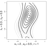
(a)

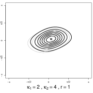
(b)

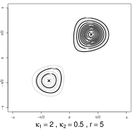
(c)

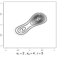
(d)

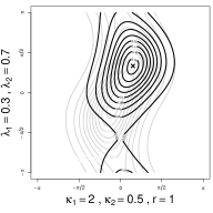
(e)

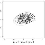
(f)

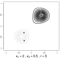
(g)

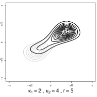
(h)

Figure 1: Bivariate sine-skewed Sine density functions (with $\bm{\mu}=\bm{0}$), where the gray contour indicates the symmetric bivariate Sine density ($\lambda_{1}=\lambda_{2}=0$) and the dark contour the sine-skewed version obtained for the skewness parameters indicated at the left. The other parameters are indicated in the labels.
From left to right: effect of the concentration and dependence parameters. From top to bottom: effect of the skewness parameters. The crosses identify the mode locations.

Let us now calculate the density of the first marginal. To this end, we denote by $a(x_{1})$ and $b(x_{1})$ the quantities such that $\kappa_{2}=a(x_{1})\cos(b(x_{1}))$ and $r\sin(x_{1}-\mu_{1})=a(x_{1})\sin(b(x_{1}))$. Then, using integration results involving the already mentioned modified Bessel function of order 0, $I_{0}$, as well as the modified Bessel function of order 1, $I_{1}$, we get

$$g_{1;\tiny{\mbox{SS}}}(x_{1}-\mu_{1};{\mu_{2}},\bm{\kappa},r,\bm{\lambda}) = \frac{1}{C_{\bm{\kappa},r}}\exp(\kappa_{1}\cos(x_{1}-\mu_{1}))\left[2\pi I_{0}(a(x_{1}))(1+\lambda_{1}\sin(x_{1}))\right.$$ (3.1)

$$+ \left.\lambda_{2}\frac{I_{1}(a(x_{1}))}{I_{0}(a(x_{1}))}\cos(\mu_{2}+b(x_{1}))\right],$$

$$a(x_{1})^{2} = \kappa_{2}^{2}+r^{2}\sin^{2}(x_{1}-\mu_{1}),$$

$$\tan(b(x_{1})) = ({r}/{\kappa_{2}})\sin(x_{1}-\mu_{1}).$$

The second marginal can be obtained in a similar way. Regarding the first marginal, as expected from the results in Subsection 2.2, if $\lambda_{2}=0$, then the density $g_{1;\tiny{\mbox{SS}}}$ is a sine-skewed version of a symmetric density, but, in general (unless $r=0$), not a sine-skewed von Mises. If $\lambda_{1}=0$ and $\lambda_{2}\neq 0$, in general (if $r\neq 0$), the marginal density $g_{1;\tiny{\mbox{SS}}}$ is not (reflectively) symmetric.

An extension of the Sine model to the $d$-variate setting was provided by Mardia et al. (2008). The resulting $d$-variate sine-skewed Sine density is given by

$$g_{\tiny{\mbox{SS}}}(\bm{x}-\bm{\mu};\bm{\kappa},\bm{R},\bm{\lambda}) = \frac{1}{C_{\bm{\kappa},\bm{R}}}\exp(\bm{\kappa}^{T}c(\bm{x},\bm{\mu})+s(\bm{x},\bm{\mu})^{T}\bm{R}s(\bm{x},\bm{\mu}))\left(1+\bm{\lambda}^{T}s(\bm{x},\bm{\mu})\right),$$

$$c(\bm{x},\bm{\mu}) = (\cos(x_{1}-\mu_{1}),\ldots,\cos(x_{d}-\mu_{d}))^{T},$$

$$s(\bm{x},\bm{\mu}) = (\sin(x_{1}-\mu_{1}),\ldots,\sin(x_{d}-\mu_{d}))^{T},$$

$$R_{i,j} = R_{j,i},\quad-\infty<R_{i,j}<\infty,\quad R_{i,i}=0,\quad i,j\in\{1,\ldots,d\},$$

where $\bm{\mu}\in\mathbb{T}^{d}$, $\bm{\kappa}\in(\mathbb{R}^{+})^{d}$, $\bm{\lambda}\in[-1,1]^{d}$ with $\sum_{s=1}^{d}|\lambda_{s}|\leq 1$ and where, in general, the analytic expression of the normalizing constant $C_{\bm{\kappa},\bm{R}}$ is unknown when $d>2$.

3.3 Sine-skewed Cosine distribution

Another popular submodel of the bivariate density of Mardia (1975) is the so-called Cosine model of Mardia et al. (2007). A comparison between both models (Sine and Cosine) can be found in Mardia et al. (2007). Again five parameters are needed for the original density, and two are introduced as skewness parameters $\lambda_{1},\lambda_{2}\in[-1,1]$ subject to $|\lambda_{1}|+|\lambda_{2}|\leq 1$. The sine-skewed Cosine density then reads

$$g_{\tiny{\mbox{SC}}}(\bm{x}-\bm{\mu};\bm{\kappa},r,\bm{\lambda}) = C_{\bm{\kappa},r}^{-1}\exp(\kappa_{1}\cos(x_{1}-\mu_{1})+\kappa_{2}\cos(x_{2}-\mu_{2})+r\cos(x_{1}-\mu_{1}-x_{2}+\mu_{2}))$$

$$\times (1+\lambda_{1}\sin(x_{1}-\mu_{1})+\lambda_{2}\sin(x_{2}-\mu_{2}))\mbox{, with}$$

$$C_{\bm{\kappa},r} = 4\pi^{2}\left(I_{0}(\kappa_{1})I_{0}(\kappa_{2})I_{0}(r)+2\sum_{i=1}^{\infty}I_{i}(\kappa_{1})I_{i}(\kappa_{2})I_{i}(r)\right).$$

For the original symmetric case $\bm{\lambda}=\bm{0}$, unimodality will depend on the values of $\bm{\kappa}$ and $r$, holding when $-r<\kappa_{1}\kappa_{2}/(\kappa_{1}+\kappa_{2})$ (see Mardia et al., 2007, Theorem 2). In this case, since the concentration parameters are always positive, unimodality will hold if also $r$ is positive. Plots of its sine-skewed version are provided in Figure 2. As shown on the bottom-left panel, even when $r>0$, unimodality may not hold for the sine-skewed Cosine distribution.

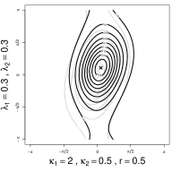
(a)

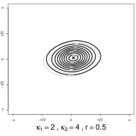
(b)

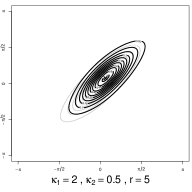
(c)

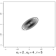
(d)

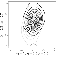
(e)

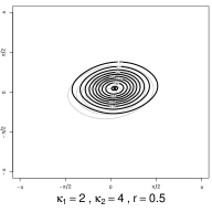
(f)

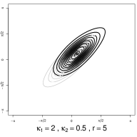
(g)

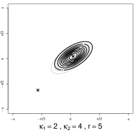
(h)

Figure 2: Bivariate sine-skewed Cosine density functions (with $\bm{\mu}=\bm{0}$), where the gray contour indicates the symmetric bivariate Cosine density ($\lambda_{1}=\lambda_{2}=0$) and the dark contour the sine-skewed version obtained for the skewness parameters indicated at the left. The other parameters are indicated in the labels.
From left to right: effect of the concentration and dependence parameters. From top to bottom: effect of the skewness parameters. The crosses identify the mode locations.

Regarding the marginals, the same density as in (3.1) is obtained, up to the value of the normalizing constant $C_{\bm{\kappa},r}$ and the values of $a(x_{1})$ and $b(x_{1})$ which, in this case, are the quantities such that $\kappa_{2}+r\cos(x_{1}-\mu_{1})=a(x_{1})\cos(b(x_{1}))$ and $r\sin(x_{1}-\mu_{1})=a(x_{1})\sin(b(x_{1}))$. Thus, similar comments as for the sine-skewed Sine distribution apply.

From the $d$-dimensional von Mises density proposed by Mardia and Patrangenaru (2005), as a particular case, the generalization of the Cosine distribution can be derived. In that case, the resulting $d$-variate sine-skewed Cosine density is

$$g_{\tiny{\mbox{SC}}}(\bm{x}-\bm{\mu};\bm{\kappa},\bm{R},\bm{\lambda}) = \frac{1}{C_{\bm{\kappa},\bm{R}}}\exp(\bm{\kappa}^{T}c(\bm{x},\bm{\mu})+s(\bm{x},\bm{\mu})^{T}\bm{R}s(\bm{x},\bm{\mu})+c(\bm{x},\bm{\mu})^{T}\bm{R}c(\bm{x},\bm{\mu}))$$

$$\times \left(1+\bm{\lambda}^{T}s(\bm{x},\bm{\mu})\right),$$

$$R_{i,j} = R_{j,i},\quad-\infty<R_{i,j}<\infty,\quad R_{i,i}=0,\quad i,j\in\{1,\ldots,d\},$$

where $\bm{\mu}\in\mathbb{T}^{d}$, $\bm{\kappa}\in(\mathbb{R}^{+})^{d}$ and $\bm{\lambda}\in[-1,1]^{d}$ with $\sum_{s=1}^{d}|\lambda_{s}|\leq 1$.

3.4 Bivariate sine-skewed wrapped Cauchy distribution

While Sine and Cosine models focus on having conditional von Mises densities, inherited logically from the bivariate von Mises distribution, Kato and Pewsey (2015) provide a way of constructing toroidal densities focusing on the wrapped Cauchy distribution. Starting from their density, the sine-skewed bivariate wrapped Cauchy distribution corresponds to

$$g_{\tiny{\mbox{SWC}}}(\bm{x}-\bm{\mu};\bm{\kappa},r,\bm{\lambda}) = (1-r^{2})(1-\kappa_{1}^{2})(1-\kappa_{2}^{2})[4\pi^{2}(c_{0}-c_{1}\cos(x_{1}-\mu_{1})-c_{2}\cos(x_{2}-\mu_{2})$$ (3.2)

$$- c_{3}\cos(x_{1}-\mu_{1})\cos(x_{2}-\mu_{2})-c_{4}\sin(x_{1}-\mu_{1})\sin(x_{2}-\mu_{2}))]^{-1}$$

$$\times (1+\lambda_{1}\sin(x_{1}-\mu_{1})+\lambda_{2}\sin(x_{2}-\mu_{2})),$$

$$c_{0} = (1+r^{2})(1+\kappa_{1}^{2})(1+\kappa_{2}^{2})-8|r|\kappa_{1}\kappa_{2},$$

$$c_{1} = 2(1+r^{2})\kappa_{1}(1+\kappa_{2}^{2})-4|r|(1+\kappa_{1}^{2})\kappa_{2},$$

$$c_{2} = 2(1+r^{2})(1+\kappa_{1}^{2})\kappa_{2}-4|r|\kappa_{1}(1+\kappa_{2}^{2}),$$

$$c_{3} = -4(1+r^{2})\kappa_{1}\kappa_{2}+2|r|(1+\kappa_{1}^{2})(1+\kappa_{2}^{2}),$$

$$c_{4} = 2r(1-\kappa_{1}^{2})(1-\kappa_{2}^{2}),$$

with location parameter $\bm{\mu}\in\mathbb{T}^{2}$, concentration parameter $\bm{\kappa}\in[0,1)^{2}$, skewness parameter $\bm{\lambda}\in[-1,1]^{2}$ subject to with $|\lambda_{1}|+|\lambda_{2}|\leq 1$, and dependence parameter $-1<r<1$. The contour plots of the density (3.2) for different values of these parameters are shown in Figure 3.

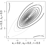
(a)

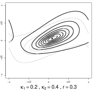
(b)

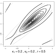
(c)

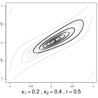
(d)

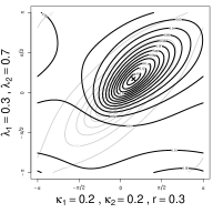
(e)

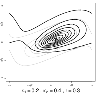
(f)

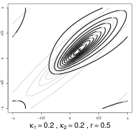
(g)

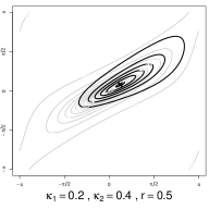
(h)

Figure 3: Bivariate sine-skewed wrapped Cauchy density functions (with $\bm{\mu}=\bm{0}$), where the gray contour indicates the symmetric bivariate wrapped Cauchy density ($\lambda_{1}=\lambda_{2}=0$) and the dark contour the sine-skewed version obtained for the skewness parameters indicated at the left. The other parameters are indicated in the labels.
From left to right: effect of the concentration and dependence parameters. From top to bottom: effect of the skewness parameters. The crosses identify the mode locations.

The marginal distributions of the model by Kato and Pewsey (2015) are univariate wrapped Cauchy distributions. From the different (non-uniform) base symmetric densities investigated by Abe and Pewsey (2011) for the univariate case, the wrapped Cauchy is the only one providing always unimodal sine-skewed alternatives. In Kato and Pewsey (2015), it is mentioned that the bivariate wrapped Cauchy is always unimodal when $\kappa_{1},\kappa_{2}>0$. This persistent unimodality feature is not inherited in the bivariate sine-skewed toroidal setting. Despite the fact that, in most of the investigated cases, unimodality was obtained, this property cannot be guaranteed to hold unless both marginals are independent. A counter-example to unimodality corresponds to the following choice of parameter values: $\kappa_{1}=0.1,\kappa_{2}=0.5,r=0.5,\lambda_{1}=1$ and $\lambda_{2}=0$ (see Figure 4, left panels). Figure 4 (right panels) informs us about the behavior of the marginals. While $\lambda_{2}=0$ guarantees that the first marginal will be equivalent to the sine-skewed version of the circular wrapped Cauchy density with parameters $\kappa_{1}$ and $\lambda_{1}$, the same is not true for the second case as $\lambda_{1}\neq 0$. In this case, note also that even if $\lambda_{2}=0$, a skewed univariate marginal in the second dimension is obtained.

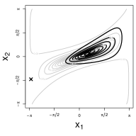
(a)

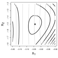
(b)

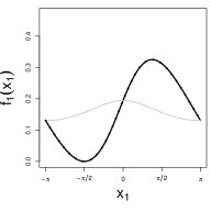
(c)

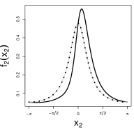
(d)

Figure 4: Bivariate sine-skewed wrapped Cauchy density functions with parameters $\bm{\mu}=\bm{0},\kappa_{1}=0.1,\kappa_{2}=0.5$ and $r=0.5$, where the dark continuous lines correspond to $\lambda_{1}=1$ and $\lambda_{2}=0$ and the gray continuous lines indicate the bivariate wrapped Cauchy density ($\lambda_{1}=\lambda_{2}=0$). The crosses identify the mode locations, and in the two right-most settings the dotted lines stand for the univariate sine-skewed densities with parameters $\kappa_{s}$ and $\lambda_{s}$.
Left: entire support $\mathbb{T}^{2}$. Center-left: close-up to show the secondary mode. Center-right: first marginal. Right: second marginal.

4 Inference

Let $\bm{\mathcal{X}}=(\bm{X}_{1},\ldots,\bm{X}_{n})$, with $\bm{X}_{i}=({X}_{i;1},\ldots,{X}_{i;d})^{T}$, denote a random sample of $d$-toroidal data generated by the distribution associated to the sine-skewed toroidal density (2.1). The objective of this section is to explain how to estimate the various parameters, derive the asymptotic properties of the estimates and build a test for symmetry against sine-skewedness.

If the trigonometric moments of the base symmetric density are known, the method of moments estimators can easily be obtained by equating the expressions of the shape parameters (see Subsection 2.2) with their sample counterparts. The main issue of this approach is that, even for the univariate case, the solutions of those equations need not necessarily exist (see Abe and Pewsey, 2011, Subsection 4.3). For that reason, in the remainder of this section, we will focus on the maximum likelihood estimators.

4.1 Maximum likelihood estimation

Given a base density $f(\bm{x}-\bm{\mu};\bm{\vartheta})$, the log-likelihood function of its sine-skewed counterpart is given by

$$\ell(\bm{\mu},\bm{\vartheta},\bm{\lambda})=\sum_{i=1}^{n}\log\left(1+\sum_{s=1}^{d}\lambda_{s}\sin(X_{i;s}-\mu_{s})\right)+\sum_{i=1}^{n}\log f(\bm{X}_{i}-\bm{\mu};\bm{\vartheta}),$$ (4.1)

whose maximization with respect to $\bm{\mu},\bm{\vartheta},\bm{\lambda}$ yields the maximum likelihood estimates (MLEs). Closed-form expressions in general do not exist for the MLEs, and we have to revert to numerical methods able to deal with a nonlinear optimization problem since we need to satisfy the constraint $\sum_{s=1}^{d}|\lambda_{s}|\leq 1$. We use the solver proposed by Ye (1987) implemented in the Rsolnp package (Ghalanos and Theussl, 2015) of the statistical software $\mathtt{R}$, and suggest to use different initial points to avoid having a local maximum as a solution.

4.2 Asymptotic behavior of the maximum likelihood estimators

Denote by $(\bm{\mu}_{0},\bm{\vartheta}_{0},\bm{\lambda}_{0})$ the true parameter values and suppose that they lie in the interior of their domain. Then, from Equation (4.1), we can see that if the base density satisfies the assumptions for asymptotic normality results on the MLE of $\bm{\mu},\bm{\vartheta}$ (see Van der Vaart, 2000, Theorem 5.39 or the classical conditions in Subsection 5.6), then its sine-skewed counterpart will also satisfy them. We thus have

$$\sqrt{n}\left((\hat{\bm{\mu}}^{T},\hat{\bm{\vartheta}}^{T},\hat{\bm{\lambda}}^{T})^{T}-(\bm{\mu}_{0}^{T},\bm{\vartheta}_{0},^{T}\bm{\lambda}_{0}^{T})^{T}\right)\overset{d}{\rightarrow}N\left(\bm{0},\mathfrak{I}^{-1}\right),$$

where $\overset{d}{\rightarrow}$ represents convergence in distribution and $\mathfrak{I}$ denotes the Fisher Information matrix. The elements of that symmetric matrix $\mathfrak{I}$ are equal to

$$\mathfrak{i}_{\mu_{j},\mu_{k}} = \mathfrak{i}_{\mu_{j},\mu_{k}}^{0}+\int_{\mathbb{T}^{d}}{\frac{\lambda_{j}\lambda_{k}\cos(x_{j})\cos(x_{k})}{1+\sum_{s=1}^{d}\lambda_{s}\sin(x_{s})}f(\bm{x};\bm{\vartheta})}d\bm{x},$$

$$\mathfrak{i}_{\mu_{j},\lambda_{k}} = \int_{\mathbb{T}^{d}}{\frac{\lambda_{j}\cos(x_{j})\sin(x_{k})}{1+\sum_{s=1}^{d}\lambda_{s}\sin(x_{s})}f(\bm{x};\bm{\vartheta})}d\bm{x},$$

$$\mathfrak{i}_{\mu_{j},\vartheta_{k}} = \mathfrak{i}_{\mu_{j},\vartheta_{k}}^{0}+\sum_{s=1}^{d}\lambda_{s}\int_{\mathbb{T}^{d}}\frac{\sin(x_{s})}{f(\bm{x};\bm{\vartheta})}\frac{\partial}{\partial x_{j}}f(\bm{x};\bm{\vartheta})\frac{\partial}{\partial\vartheta_{k}}f(\bm{x};\bm{\vartheta})d\bm{x},$$

$$\mathfrak{i}_{\lambda_{j},\lambda_{k}} = \int_{\mathbb{T}^{d}}{\frac{\sin(x_{j})\sin(x_{k})}{1+\sum_{s=1}^{d}\lambda_{s}\sin(x_{s})}f(\bm{x};\bm{\vartheta})}d\bm{x},$$

$$\mathfrak{i}_{\lambda_{j},\vartheta_{k}} = 0,$$

$$\mathfrak{i}_{\vartheta_{j},\vartheta_{k}} = \mathfrak{i}_{\vartheta_{j},\vartheta_{k}}^{0}+\sum_{s=1}^{d}\lambda_{s}\int_{\mathbb{T}^{d}}\frac{\sin(x_{s})}{f(\bm{x};\bm{\vartheta})}\frac{\partial}{\partial\vartheta_{j}}f(\bm{x};\bm{\vartheta})\frac{\partial}{\partial\vartheta_{k}}f(\bm{x};\bm{\vartheta})d\bm{x},$$

where the elements of $\mathfrak{I}$ with a superscript 0 denote the values of the corresponding elements of the Fisher Information matrix for the base density.

4.3 Testing for symmetry

A question of natural interest in our investigation is whether the sine-skewed models indeed improve significantly on their symmetric antecedents for a given sample $\bm{\mathcal{X}}$. This boils down to testing for the nested symmetry inside a sine-skewed toroidal distribution, which can be formulated as the hypothesis testing problem

$$H_{0}:\bm{\lambda}=\bm{0}\quad\mbox{versus}\quad H_{1}:\bm{\lambda}\neq\bm{0}.$$

A likelihood ratio test is a straightforward and efficient procedure to tackle this problem. For each parameter $\bm{\psi}\in\{\bm{\mu},\bm{\vartheta},\bm{\lambda}\}$, we denote as before by $\hat{\bm{\psi}}$ the unconstrained maximum likelihood estimate and by $\hat{\bm{\psi}}_{0}$ the maximum likelihood estimate under the null hypothesis of symmetry (i.e., the MLEs from the base symmetric distribution). The likelihood ratio test then rejects the null hypothesis at asymptotic level $\alpha$ whenever the test statistic $-2(\ell(\hat{\bm{\mu}}_{0},\hat{\bm{\vartheta}}_{0},\bm{0})-\ell(\hat{\bm{\mu}},\hat{\bm{\vartheta}},\hat{\bm{\lambda}}))$ exceeds $\chi^{2}_{d;1-\alpha}$, the $\alpha$-upper quantile of a chi-square distribution with $d$ degrees of freedom.

5 Application on protein data

Modeling the three-dimensional structure of proteins has become a topic of special interest in the protein bioinformatics field. Proteins are constructed from a linear sequence of monomers, called amino acids. The folded structure of a protein is determined by its amino acid sequence. The relative orientation of subsequent amino acids can be described by the pairs of dihedral angles $\phi$ and $\psi$, which correspond to the rotations of the ${\rm N}-{\rm C}_{\alpha}$ and ${\rm C}_{\alpha}-{\rm C}^{\prime}$ bonds in the backbone of the protein. A more detailed biochemical background for analyzing protein structures can be found in Mardia et al. (2018). In this section, our objective is to use the proposed bivariate sine-skewed toroidal distributions to model the pairs of dihedral angles on the different types of amino acids.

The analyzed dataset was obtained from the Top500 database, a selection of 500 files from the Protein Data Bank that are high resolution ($1.8\mathring{A}$ or better), low homology, and high quality (see http://kinemage.biochem.duke.edu/databases/top500.php for details). In the employed data, all proteins with chain breaks and PDB files that caused errors upon parsing were removed, resulting in data on 402 proteins. Also, the amino acids with a C- or N-terminus are not employed as they do not have one of the corresponding rotation-angles. Then, for each type of amino acid, since there may be a dependency between two amino acids that are part of the same protein, just one pair of rotation-angle was selected for each protein.

	Model	Comp	$\hat{\mu}_{1}$	$\hat{\mu}_{2}$	$\hat{\kappa}_{1}$	$\hat{\kappa}_{2}$	$\hat{r}$	$\hat{\lambda}_{1}$	$\hat{\lambda}_{2}$	$\hat{p}$	LL	AIC	BIC
S ($n=396$)	S	1	-1.8	2.493	2.215	2.116	-0.094	–	–	0.607	-780.5	1583.1	1626.9
		2	-1.225	-0.486	38.466	29.498	-23.664	–	–	0.393
	SS	1	-1.338	-0.389	17.805	19.977	-13.535	0.168	-0.582	0.442	-725.1*	1480.1	1539.8
		2	2.903	1.222	0.016	0.986	4.446	0.014	0.985	0.558
	C	1	-1.879	2.529	1.578	1.502	0.843	–	–	0.589	-814.1	1650.1	1693.9
		2	-1.224	-0.486	23.795	14.28	0	–	–	0.411
	SC	1	-1.393	-0.474	8.333	8.555	0	0.776	0.182	0.45	-811.6	1653.1	1712.8
		2	-2.384	2.335	0.268	3.393	1.801	0.945	-0.018	0.55
	WC	1	-1.787	2.637	0.604	0.788	-0.036	–	–	0.539	-764	1550	1593.8
		2	-1.17	-0.567	0.865	0.789	-0.44	–	–	0.461
	SWC	1	-1.311	2.631	0.639	0.801	-0.129	-1	0	0.524	-717*	1464	1523.7
		2	-1.144	-0.638	0.844	0.78	-0.51	0.039	0.961	0.476
G ($n=399$)	S	1	2.875	1.546	1.091	0.66	5.899	–	–	0.6	-1047.1	2116.3	2160.2
		2	0.269	-1.795	0.462	1.959	-6.248	–	–	0.4
	SS	1	0.277	-1.784	0.401	1.936	-6.071	-0.386	-0.234	0.403	-1041.1*	2112.2	2172.1
		2	2.895	1.53	1.086	0.702	5.988	-0.548	0.452	0.597
	C	1	0.52	-0.155	0.001	4.937	1.024	–	–	0.522	-1233	2488	2531.8
		2	-2.733	3.111	0.631	4.086	0	–	–	0.478
	SC	1	2.598	2.748	0.001	0.631	0.568	0.493	0.506	0.712	-1220.5*	2471	2530.8
		2	1.495	-0.004	10.463	6.567	0	0.005	0.993	0.288
	WC	1	-1.42	0.504	0.603	0	-0.676	–	–	0.636	-1110.7	2243.5	2287.3
		2	1.443	0.039	0.819	0.741	-0.542	–	–	0.364
	SWC	1	1.385	0.121	0.816	0.723	-0.536	1	0	0.383	-1079*	2188.1	2247.9
		2	-1.328	0.371	0.647	0	-0.665	-0.786	-0.214	0.617
P ($n=390$)	S	1	-1.169	2.557	32.752	9.399	-4.165	–	–	0.603	-173.4	368.9	412.5
		2	-1.133	-0.415	73.17	46.121	-51.988	–	–	0.397
	SS	1	-1.686	-2.256	33.22	0.79	-20.318	0	-1	0.607	-150.1*	330.1	389.6
		2	-1.165	-0.364	81.556	49.781	-57.897	0	-1	0.393
	C	1	-1.111	-0.44	15.2	13.869	0.005	–	–	0.421	-285.5	593.1	636.7
		2	-1.17	2.612	29.292	7.04	0	–	–	0.579
	SC	1	-1.112	-0.441	15.201	13.869	0	0.689	0.136	0.421	-282.2	594.5	654
		2	-1.17	2.613	29.292	7.04	0.001	0.147	-0.561	0.579
	WC	1	-1.143	2.589	0.884	0.857	-0.416	–	–	0.595	-191.1	404.2	447.8
		2	-1.067	-0.494	0.881	0.822	-0.583	–	–	0.405
	SWC	1	-1.115	2.568	0.883	0.857	-0.425	-1	0	0.594	-178.8*	387.5	447
		2	-1.039	-0.548	0.882	0.819	-0.586	0	1	0.406

Table 1: Parameter estimation for each component, log-likelihood (LL), AIC and BIC of the mixture of Sine (S), Cosine (C) and wrapped Cauchy (WC) distributions and their sine-skewed versions (respectively, SS, SC, SWC). In the LL value of the sine-skewed models, an asterisk (*) indicates when the null hypothesis of symmetry is rejected against the sine-skewed version at the level $\alpha=0.01$. Each block corresponds to one amino acid type, from top to bottom: serine (S), glycine (G) and proline (P).

Amino acid	A	C	D	E	F	G	H	I	K	L
Model	SWC	SWC	SS	SWC	SS	SS/S	SS	SWC	SWC	SWC
Amino acid	M	N	P	Q	R	S	T	V	W	Y
Model	SWC	SS	SS	SWC	SWC	SWC	SS/S	SWC	SWC	SS

Table 2: Model providing the best fit on the basis of the AIC/BIC for each amino acid type. For G and T, a distinct model is obtained according to AIC and BIC.

From the total of 20 amino acid types, in this section, we focus on three of them as all of them present a similar pattern except for the glycine (G symbol) and proline (P symbol). The amino acid type chosen to represent the rest of them is the serine (S symbol). The full analysis of the 20 different amino acid types is provided in Section LABEL:extra_protein of the Supplementary Material. The scatter (planar) plot of the toroidal protein data, also known as Ramachandran plot (Ramachandran, 1963) in the protein bioinformatics field, is represented in Figure 5 for each amino acid type (see also the figures from Section LABEL:extra_protein of the Supplementary Material). The Ramachandran plot suggests that at least a bimodal distribution is needed. For that reason, the following mixture of two toroidal densities was employed:

$$g_{M}(\bm{x};\bm{\mu}_{1},\bm{\mu}_{2},\bm{\vartheta}_{1},\bm{\vartheta}_{2},\bm{\lambda}_{1},\bm{\lambda}_{2},p)=pg_{1}(\bm{x}-\bm{\mu}_{1};\bm{\vartheta}_{1},\bm{\lambda}_{1})+(1-p)g_{2}(\bm{x}-\bm{\mu}_{2};\bm{\vartheta}_{2},\bm{\lambda}_{2}),$$ (5.1)

where $p\in[0,1]$ and $g_{j}$, with $j\in\{1,2\}$, are two sine-skewed densities of the form (2.1). The parameter estimates are obtained via the optimization approach described in Subsection 4.1, after having adapted the optimization algorithm such that it takes into account the constraints of both mixture components and $0\leq p\leq 1$. As base symmetric densities, we considered the three non-uniform distributions described in Section 3: the bivariate Sine, Cosine and wrapped Cauchy distributions. For comparative purposes, we also computed the MLEs of the mixtures of these symmetric distributions, corresponding to $\bm{\lambda}_{1}=\bm{\lambda}_{2}={\boldsymbol{0}}$ in (5.1). In Table 1 we provide, for every amino acid type, the sample size, the MLEs, the maximum value of the log-likelihood function (LL), the Akaike Information Criterion (AIC) and the Bayesian Information Criterion (BIC) for each model. The test of symmetry described in Subsection 4.3 is applied at significance level $\alpha=0.01$ and the rejection of the null hypothesis is indicated in Table 1 with an asterisk in the LL value. As we can see, in most cases the sine-skewed version improves on the original symmetric density, and for each amino acid type a sine-skewed toroidal distribution provides the best fit in terms of AIC: for S it is the sine-skewed wrapped Cauchy model, for G and P the sine-skewed Sine model. Regarding the BIC, for S and P, it is the same models, while for G the base Sine model has the lowest value. Table 2 includes a summary indicating which is the best model in terms of AIC and BIC for all amino acid types, hence also those not treated here but in the Supplementary Material. We also see that in most cases the null hypothesis of symmetry is rejected at a significance level $\alpha=0.01$. Thus, it is clear that the proposed sine-skewing transformation of this paper strongly improves the goodness-of-fit without overfitting the data.

The graphical representation of the fitted models is provided in Figure 5, and the Supplementary Material contains the figures corresponding to the remaining amino acid types. A common trait of all figures is that we can see that the best-fitting mixture of sine-skewed toroidal distributions corresponds to a very good fit of the data points in the Ramachandran plot.

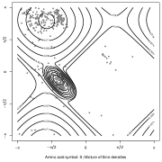
(a)

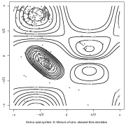
(b)

(c)

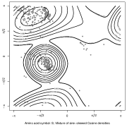
(d)

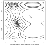
(e)

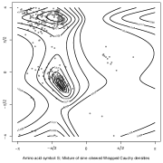
(f)

(g)

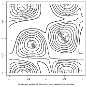
(h)

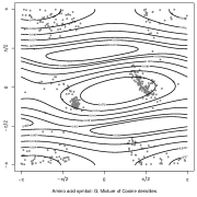
(i)

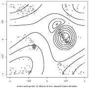
(j)

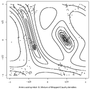
(k)

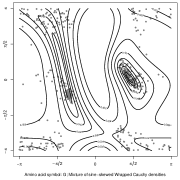
(l)

(m)

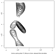
(n)

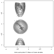
(o)

(p)

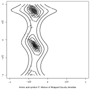
(q)

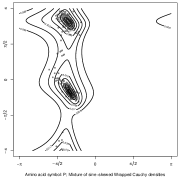
(r)

Figure 5: Ramachandran plot (gray points) and maximum likelihood fits (black contour) of mixtures of the base models and of mixtures of their sine-skewed versions for the protein data. The studied amino acid types are: serine (S), glycine (G) and proline (P).

6 Conclusion

In this paper, we have introduced the sine-skewed toroidal distributions, which are obtained by applying our sine-skewing transformation to any existing symmetric distribution on the torus. It is a very general way of allowing distributions to take into account potential skewness occurring in real data sets, and its simple implementation allows future researchers to immediately also build sine-skewed versions of their new distributions. We have thus filled a long-standing gap in the literature that had been identified by various authors such as Mardia (2013). Our proposal enjoys several nice features: the construction is simple, especially thanks to the absence of need to calculate a normalizing constant, the random number generation is very easy, trigonometric moments are readily obtained from the initial symmetric toroidal distribution, parameter estimation via maximum likelihood works well, and highly versatile shapes can be attained by sine-skewed toroidal distributions. A potential drawback, which is however shared by most distributions on the torus, is that unimodality cannot be always guaranteed.

We have seen in Section 5 the improved fit to dihedral angle data provided by sine-skewed toroidal distributions in comparison to the popular existing symmetric distributions. As mentioned in the Introduction, toroidal distributions are playing an increasingly important role in protein bioinformatics, in particular in the protein structure prediction problem. The sine-skewed transformation promises a crucial step forward in this active research area, and it is currently being implemented in the software $\mathtt{R}$ and Pyro to allow a user-friendly usage.

See pages - of SM_sine_skewed_v3.pdf

References

- Abe and Pewsey (2011) Abe, T. and A. Pewsey (2011). Sine-skewed circular distributions. Statistical Papers 52, 683–707.
- Azzalini (1985) Azzalini, A. (1985). A class of distributions which includes the normal ones. Scandinavian journal of statistics 12, 171–178.
- Azzalini and Dalla Valle (1996) Azzalini, A. and A. Dalla Valle (1996). The multivariate skew-normal distribution. Biometrika 83, 715–726.
- Boomsma et al. (2008) Boomsma, W., K. V. Mardia, C. C. Taylor, J. Ferkinghoff-Borg, A. Krogh, and T. Hamelryck (2008). A generative, probabilistic model of local protein structure. Proceedings of the National Academy of Sciences 105, 8932–8937.
- Downs and Mardia (2002) Downs, T. D. and K. V. Mardia (2002). Circular regression. Biometrika 89, 683–697.
- Fernández-Duran (2007) Fernández-Duran, J. J. (2007). Models for circular-linear and circular-circular data constructed from circular distributions based on nonnegative trigonometric sums. Biometrics 63, 579–585.
- Fisher and Lee (1983) Fisher, N. I. and A. J. Lee (1983). A correlation coefficient for circular data. Biometrika 70, 327–332.
- García-Portugués et al. (2019) García-Portugués, E., M. Sörensen, K. V. Mardia, and T. Hamelryck (2019). Langevin diffusions on the torus: estimation and applications. Statistics and Computing 29, 1–22.
- Ghalanos and Theussl (2015) Ghalanos, A. and S. Theussl (2015). Rsolnp: General Non-linear Optimization Using Augmented Lagrange Multiplier Method. R package version 1.16.
- Hamelryck et al. (2012) Hamelryck, T., K. V. Mardia, and J. Ferkinghoff-Borg (Eds.) (2012). Bayesian Methods in Structural Bioinformatics. Heidelberg, Germany: Springer.
- Harder et al. (2010) Harder, T., W. Boomsma, M. Paluszewski, J. Frellsen, K. E. Johansson, and T. Hamelryck (2010). Beyond rotamers: a generative, probabilistic model of side chains in proteins. BMC Bioinformatics 11, 306.
- Johnson and Wehrly (1977) Johnson, R. A. and T. E. Wehrly (1977). Measures and models for angular correlation and angular-linear correlation. Journal of the Royal Statistical Society: Series B (Methodological) 39, 222–229.
- Jones et al. (2015) Jones, M. C., A. Pewsey, and S. Kato (2015). On a class of circulas: copulas for circular distributions. Annals of the Institute of Statistical Mathematics 67, 843–862.
- Jupp et al. (2016) Jupp, P. E., G. Regoli, and A. Azzalini (2016). A general setting for symmetric distributions and their relationship to general distributions. Journal of Multivariate Analysis 148, 107–119.
- Kato (2009) Kato, S. (2009). A distribution for a pair of unit vectors generated by Brownian motion. Bernoulli 15, 898–921.
- Kato and Pewsey (2015) Kato, S. and A. Pewsey (2015). A Möbius transformation-induced distribution on the torus. Biometrika 102, 359–370.
- Kato et al. (2008) Kato, S., K. Shimizu, and G. S. Shieh (2008). A circular–circular regression model. Statistica Sinica 18, 633–645.
- Kent et al. (2008) Kent, J. T., K. V. Mardia, and C. C. Taylor (2008). Modelling strategies for bivariate circular data. In S. Barber, P. D. Baxter, A. Gusnanto, and K. V. Mardia (Eds.), Proceedings of the Leeds Annual Statistical Research Conference, The Art and Science of Statistical Bioinformatics, Leeds University Press, Leeds, pp. 70–73.
- Ley and Verdebout (2017a) Ley, C. and T. Verdebout (2017a). Modern Directional Statistics. Boca Ratón, Florida: Chapman and Hall/CRC Press.
- Ley and Verdebout (2017b) Ley, C. and T. Verdebout (2017b). Skew-rotationally-symmetric distributions and related efficient inferential procedures. Journal of Multivariate Analysis 159, 67–81.
- Ley and Verdebout (2019) Ley, C. and T. Verdebout (Eds.) (2019). Applied Directional Statistics: Modern Methods and Case Studies. Boca Ratón, Florida: Chapman and Hall/CRC Press.
- Mardia (1975) Mardia, K. V. (1975). Statistics of directional data. Journal of the Royal Statistical Society: Series B (Methodological) 37, 349–371.
- Mardia (2013) Mardia, K. V. (2013). Statistical approaches to three key challenges in protein structural bioinformatics. Journal of the Royal Statistical Society: Series C (Applied Statistics) 62, 487–514.
- Mardia et al. (2018) Mardia, K. V., J. I. Foldager, and J. Frellsen (2018). Applied Directional Statistics: Modern Methods and Case Studies, Chapter Directional Statistics in Protein Bioinformatics. Boca Ratón, Florida: Chapman and Hall/CRC Press.
- Mardia et al. (2008) Mardia, K. V., G. Hughes, C. C. Taylor, and H. Singh (2008). A multivariate von Mises distribution with applications to bioinformatics. Canadian Journal of Statistics 36, 99–109.
- Mardia and Jupp (2000) Mardia, K. V. and P. E. Jupp (2000). Directional Statistics. Chichester, United Kingdom: John Wiley & Sons.
- Mardia and Patrangenaru (2005) Mardia, K. V. and V. Patrangenaru (2005). Directions and projective shapes. The Annals of Statistics 33, 1666–1699.
- Mardia et al. (2007) Mardia, K. V., C. C. Taylor, and G. K. Subramaniam (2007). Protein bioinformatics and mixtures of bivariate von Mises distributions for angular data. Biometrics 63, 505–512.
- Ramachandran (1963) Ramachandran, G. N. (1963). Stereochemistry of polypeptide chain configurations. Journal of Molecular Biology 7, 95–99.
- Rivest (1988) Rivest, L.-P. (1988). A distribution for dependent unit vectors. Communications in Statistics-Theory and Methods 17, 461–483.
- Rivest (1997) Rivest, L.-P. (1997). A decentred predictor for circular-circular regression. Biometrika 84, 717–726.
- Shieh et al. (2011) Shieh, G. S., S. Zheng, R. A. Johnson, Y. F. Chang, K. Shimizu, C. C. Wang, and S. L. Tang (2011). Modeling and comparing the organization of circular genomes. Bioinformatics 27, 912–918.
- Singh et al. (2002) Singh, H., V. Hnizdo, and E. Demchuk (2002). Probabilistic model for two dependent circular variables. Biometrika 89, 719–723.
- Umbach and Jammalamadaka (2009) Umbach, D. and S. R. Jammalamadaka (2009). Building asymmetry into circular distributions. Statistics & Probability Letters 79, 659–663.
- Van der Vaart (2000) Van der Vaart, A. W. (2000). Asymptotic Statistics. Cambridge, United Kingdom: Cambridge University Press.
- Wang et al. (2004) Wang, J., J. Boyer, and M. G. Genton (2004). A skew-symmetric representation of multivariate distribution. Statistica Sinica 14, 1259–1270.
- Wehrly and Johnson (1980) Wehrly, T. E. and R. A. Johnson (1980). Bivariate models for dependence of angular observations and a related Markov process. Biometrika 66, 255–256.
- Ye (1987) Ye, Y. (1987). Interior algorithms for linear, quadratic, and linearly constrained non-linear programming. Ph. D. thesis, Department of ESS, Stanford University.