Optimal nonparametric multivariate change point detection and localization

Abstract

We study the multivariate nonparametric change point detection problem, where the data are a sequence of independent $p$-dimensional random vectors whose distributions are piecewise-constant with Lipschitz densities changing at unknown times, called change points. We quantify the size of the distributional change at any change point with the supremum norm of the difference between the corresponding densities. We are concerned with the localization task of estimating the positions of the change points. In our analysis, we allow for the model parameters to vary with the total number of time points, including the minimal spacing between consecutive change points and the magnitude of the smallest distributional change. We provide information-theoretic lower bounds on both the localization rate and the minimal signal-to-noise ratio required to guarantee consistent localization. We formulate a novel algorithm based on kernel density estimation that nearly achieves the minimax lower bound, save possibly for logarithm factors. We have provided extensive numerical evidence to support our theoretical findings.

Keywords: Multivariate; Nonparametric; Kernel density estimation; CUSUM; Binary segmentation; Minimax optimality.

1 Introduction

We study the nonparametric multivariate change point detection problem, where we are given a sequence of independent random vectors $\{X(t)\}_{t=1}^{T}\subset\mathbb{R}^{p}$ with unknown distributions $\{P_{t}\}_{t=1}^{T}$ such that, for an unknown sequence of change points $\{\eta_{k}\}_{k=1}^{K}\subset\{2,\ldots,T\}$ with $1=\eta_{0}<\eta_{1}<\ldots<\eta_{K}\leq T<\eta_{K+1}=T+1$, we have

$$P_{t}\neq P_{t-1}\quad\mbox{if and only if}\quad t\in\{\eta_{1},\ldots,\eta_{K}\}.$$ (1)

Our goal is to accurately estimate the number of change points $K$ and their locations.

Change point localization problems of this form arise in a variety of application areas, including biology, epidemiology, social sciences, climatology, technology diffusion, advertising, to name but a few. Due to the high demand from real-life applications, change point detection is a well-established topic in statistics with a rich literature. Some early efforts include seminal works by Wald (1945), Yao (1988), Yao and Au (1989), Yao and Davis (1986). More recently, the change point detection literature has been brought back to the spotlight due to significant methodological and theoretical advances, including Aue et al. (2009), Killick et al. (2012), Fryzlewicz (2014), Frick et al. (2014), Cho (2016), Wang and Samworth (2018), Wang et al. (2018a), among many others, in different aspects of parametric change point detection problems. See Wang et al. (2018b) for a more comprehensive review.

Most of the exiting results in the change point localization literature rely on parametric assumptions on the underlying distributions and on the nature of their changes. Despite the popularity and applicability of parametric change point detection methods, it is also important to develop more general and flexible change point localization procedures that are applicable over larger, possibly nonparametric, classes of distributions. Several efforts in this direction have been recently made for univariate data. Pein et al. (2017) proposed a version of the SMUCE algorithm (Frick et al., 2014) that is more sensitive to simultaneous changes in mean and variance; Zou et al. (2014) introduced a nonparametric estimator that can detect general distributions shifts; Padilla et al. (2018) considered a nonparametric procedure for sequential change point detection; Fearnhead and Rigaill (2018) focused on univariate mean change point detection constructing an estimator that is robust to outliers; Vanegas et al. (2019) proposed an estimator for detecting changes in pre-specified quantiles of the generative model; and Padilla et al. (2019) developed a nonparametric version of binary segmentation (e.g. Scott and Knott, 1974) based on the Kolmogorov–Smirnov statistic.

In multivariate nonparametric settings, the literature on change point analysissi comparatively limited. Arlot et al. (2012) considered a penalized kernel least squares estimator, originally proposed by Harchaoui and Cappé (2007), for multivariate change point problems and derive an oracle inequality. Garreau and Arlot (2018) obtained an upper bound on the localization rate afforded by this method, which is further improved computationally in Celisse et al. (2018). Matteson and James (2014) also proposed a methodology for multivariate nonparametric change point localization and show that that it can consistently estimate the change points. Zhang et al. (2017) provided a computationally-efficient algorithm, based on a pruning routine based on dynamic programming.

In this paper we investigate the multivariate change point localization problem in fully nonparametric settings where the underlying distributions are only assumed to have piecewise and uniformly (in $T$, the total number of time points) Lipschitz continuous densities and the magnitudes of the distributional changes are measured by the supremum norm of the differences between the corresponding densities. We formally introduce our model next.

Assumption 1 (Model setting).

Let $\{X(t)\}_{t=1}^{T}\subset\mathbb{R}^{p}$ be a sequence of independent vectors satisfying (1). Assume that, for each $t=1,\ldots,T$, the distribution $P_{t}$ has a bounded Lebesgue density function $f_{t}:\,\mathbb{R}^{p}\to\mathbb{R}$ such that

$$\max_{t=1,\ldots,T}\bigl{|}f_{t}(s_{1})-f_{t}(s_{2})\bigr{|}\leq C_{\mathrm{Lip}}\|s_{1}-s_{2}\|,\quad\mbox{for all }s_{1},s_{2}\in\mathcal{X},$$ (2)

where $\mathcal{X}\subset\mathbb{R}^{p}$ is the union of the supports of all the density functions $f_{t}$, $\|\cdot\|$ represents the $\ell_{2}$-norm, and $C_{\mathrm{Lip}}>0$ is an absolute constant. We let

$$\Delta=\min_{k=1,\ldots,K+1}\{\eta_{k}-\eta_{k-1}\}\leq T$$

denote the minimal spacing between any two consecutive change points. For each $k=1,\ldots,K$, we set

$$\kappa_{k}=\sup_{z\in\mathbb{R}^{p}}\bigl{|}f_{\eta_{k}}(z)-f_{\eta_{k}-1}(z)\bigr{|}=\|f_{\eta_{k}}-f_{\eta_{k}-1}\|_{\infty}$$

as the size of the change at the $k$th change point. Finally, we let

$$\kappa=\min_{k=1,\ldots,K}\kappa_{k}>0,$$ (3)

be the minimal such change.

The uniform Lipschitz condition (2) is a rather mild requirement on the smoothness of the underlying densities. The use of the supremum distance is a natural choice in nonparametric density estimation settings. If we assume the domain $\mathcal{X}$ to be compact, then the supremum distance is stronger than the $L_{1}$ distance (total variation distance).

The model parameters $\Delta$ and $\kappa$ are allowed to change with the total number of time points $T$. This modeling choice allows us to consider change point models for which it becomes increasingly difficult to identify and estimate the change point locations accurately as we acquire more data. For simplicity, we will not explicitly express the dependence of $\Delta$ and $\kappa$ on $T$ in our nation. The dimension $p$ is instead treated as a fixed constant, as is customary in nonparametric literature, although our analysis could be extended to allow $p$ to grow with $T$ with a more careful tracking of the constants; see, e.g. McDonald (2017). We will refer to any relationship among $\Delta$ and $\kappa$ that holds as $T$ tends to infinity as a parameter scaling of the model in 1.

The change point localization task can be formally stated as follows. We seek to construct change point estimators $1<\hat{\eta}_{1}<\ldots<\hat{\eta}_{\widehat{K}}\leq T$ of the true change points $\{\eta_{k}\}_{k=1}^{K}$ such that, with probability tending to $1$ as $T\rightarrow\infty$,

$$\widehat{K}=K\quad\text{and}\quad\max_{k=1,\ldots,K}|\hat{\eta}_{k}-\eta_{k}|\leq\epsilon,$$

where $\epsilon=\epsilon(T,\Delta,\kappa)$. We say that the change point estimators $\{\hat{\eta}_{k}\}_{k=1}^{\hat{K}}$ are consistent if the above holds with

$$\lim_{T\rightarrow\infty}\epsilon/\Delta=0.$$ (4)

We refer to $\epsilon$ as the localization error and to the sequence $\{\epsilon/\Delta\}$ as the localization rate.

1.1 Summary of the results

The contributions of this paper are as follows.

• We show that the difficulty of the localization task can be completely characterized in terms of the signal-to-noise ratio $\kappa^{p+2}\Delta$. Specifically, the space of the model parameters $(T,\Delta,\kappa)$ can be separated into an infeasible region, characterized by the scaling

  $$\kappa^{p+2}\Delta\lesssim 1$$ (5)

  and where no algorithm is guaranteed to produce consistent estimators of the change points (see Lemma 2), and a feasible region, in which

  $$\kappa^{p+2}\Delta\gtrsim\log^{1+\xi}(T),\quad\text{for any }\xi>0.$$ (6)

  Under the feasible scaling, we develop the MNP (multivariate nonparametric) change point estimator, given in Algorithm 1, that is provably consistent. The gap between (5) and (6) is a poly-logarithmic factor in $T$, which implies that our procedure is consistent under nearly all scalings for which this task is feasible.

• We show that the localization error achieved by the MNP procedure is of order $\log(T)\kappa^{-(p+2)}$ across the entire feasibility region given in (6); see Theorem 1. We verify that this rate is nearly minimax optimal by deriving an information-theoretic lower bound on the localization error, showing that if $\kappa^{p+2}\Delta\gtrsim\zeta_{T}$, for any sequence $\{\zeta_{T}\}$ satisfying $\lim_{T\to\infty}\zeta_{T}=\infty$, then the localization error is larger than $\kappa^{-(p+2)}$, up to constants; see Lemma 3. Interestingly, the dependence on the dimension $p$ is exponential, and matches the optimal dependence in the multivariate density estimation problems assuming Lipschitz-continuous densities. We elaborate on this point further in Section 3.2. The numerical experiments in Section 4 confirm the good performance of our algorithm.

• The MNP estimator is a computationally-efficient procedure for nonparametric change point localization in multivariate settings and can be considered a multivariate nonparametric extension of the binary segmentation methodology (Scott and Knott, 1974) and its, variant wild binary segmentation (Fryzlewicz, 2014). The MNP estimator deploys a version of the CUSUM statistic (Page, 1954) based on kernel density estimators. We remark that some of our auxiliary results on consistency of kernel density estimators are obtained through non-trivial adaptation of existing techniques that allow for non-i.i.d. the data and may be of independent interest.

The rest of the paper is organized as follows. In Section 2 we introduce the MNP procedure and in Section 3 we study its consistency and optimality. Simulation experiments demonstrating the effectiveness of the MNP algorithm and its competitive performance relative to existing procedures are reported in Section 4. The proofs and technical details are left in the Appendices.

2 Methodology

Our procedures for change point detection and localization is a nonparametric extension of the traditional CUSUM statistic and it relies on kernel density estimators.

Definition 1 (Multivariate nonparametric CUSUM).

Let $\{X(i)\}_{i=1}^{T}$ be a sample in $\mathbb{R}^{p}$. For any integer triplet $(s,t,e)$ satisfying $0\leq s<t<e\leq T$ and any $x\in\mathbb{R}^{p}$, the multivariate nonparametric CUSUM statistic is defined as the function

$$x\in\mathbb{R}^{p}\mapsto\widetilde{Y}^{s,e}_{t}(x)=\sqrt{\frac{(t-s)(e-t)}{e-s}}\left\{\hat{f}_{s+1,t,h}(x)-\hat{f}_{t+1,e,h}(x)\right\},$$

where

$$\hat{f}_{s,e,h}(x)=\frac{h^{-p}}{e-s}\sum_{i=s+1}^{e}\mathpzc{k}\left(\frac{x-X(i)}{h}\right)$$ (7)

and $\mathpzc{k}(\cdot)$ is a kernel function (see e.g. Parzen, 1962). In addition, define

$$\widetilde{Y}^{s,e}_{t}=\max_{i=1,\ldots,T}\left|\widetilde{Y}^{s,e}_{t}(X(i))\right|.$$ (8)

Remark 1.

The statistic $\widetilde{Y}^{s,e}_{t}$ can be seen as an estimator of

$$\sup_{z\in\mathbb{R}^{p}}\left|\widetilde{Y}^{s,e}_{t}(z)\right|.$$

Algorithm 1 below presents a multivariate nonparametric version of the univariate nonparametric change point detection method proposed in Padilla et al. (2019), wild binary segmentation (Fryzlewicz, 2014) and binary segmentation (BS) (e.g. Scott and Knott, 1974). The resulting procedure consists of repeated application of the BS algorithm over random time intervals and using the multivariate nonparametric CUSUM statistic in Definition 1. The inputs of Algorithm 1 are a sequence $\{X(t)\}_{t=1,\ldots,T}$ of random vectors in $\mathbb{R}^{p}$, a tuning parameter $\tau>0$ and a bandwidth $h>0$. Detailed theoretical requirements on the values of $\tau$ and $h$ are discussed below in Section 3, and Section 4.1 offers guidance on how to select them in practice. In particular, the lengths of the sub-intervals are of order at least $h^{-p}$, where $h>0$ is the value of the bandwidth used to define the multivariate nonparametric CUSUM statistic. This is to ensure that each sub-interval will contain enough points to yield a reliable density estimator.

Furthermore, in Algorithm 1 we scan through all time points between $s_{m}+h^{-p}$ and $e_{m}-h^{-p}$ in the interval $(s_{m},e_{m})$. This is done for technical reasons, to avoid working with intervals that have insufficient data, which would be the case when $e_{m}-s_{m}$ is small.

Finally, the computational cost of the algorithm is of order $O(T^{2}M\cdot\mathrm{kernel})$, where $M$ is the number of random intervals and “kernel” stands for the computational cost of calculating the value of the kernel function evaluated at one data point. The dependence on the dimension $p$ is only through the evaluation of the kernel function.

Sample $\{X(t)\}_{t=s}^{e}\subset\mathbb{R}^{p}$, collection of intervals $\{(\alpha_{m},\beta_{m})\}_{m=1}^{M}$, tuning parameter $\tau>0$ and bandwidth $h>0$.

for $m=1,\ldots,M$ do

     $(s_{m},e_{m})\leftarrow[s,e]\cap[\alpha_{m},\beta_{m}]$

     if $e_{m}-s_{m}>2h^{-p}+1$ then

         $b_{m}\leftarrow\operatorname*{arg\,max}_{s_{m}+h^{-p}\leq t\leq e_{m}-h^{-p}}\widetilde{Y}^{s_{m},e_{m}}_{t}$

         $a_{m}\leftarrow\widetilde{Y}^{s_{m},e_{m}}_{b_{m}}$

     else

         $a_{m}\leftarrow-1$

     end if

end for

$m^{*}\leftarrow\operatorname*{arg\,max}_{m=1,\ldots,M}a_{m}$

if $a_{m^{*}}>\tau$ then

     add $b_{m^{*}}$ to the set of estimated change points

     MNP$((s,b_{m*}),\{(\alpha_{m},\beta_{m})\}_{m=1}^{M},\tau)$

     MNP$((b_{m*}+1,e),\{(\alpha_{m},\beta_{m})\}_{m=1}^{M},\tau)$

end if

The set of estimated change points.

Algorithm 1 Multivariate Nonparametric Change Point Detection. MNP $((s,e),\{(\alpha_{m},\beta_{m})\}_{m=1}^{M},\tau,h)$

3 Theory

In this section we prove that the change point estimator MNP returned by Algorithm 1 is consistent based on the model described in 1, under the parameter scaling

$$\kappa^{p+2}\Delta\gtrsim\log^{1+\xi}(T),$$

for any $\xi>0$; see Theorem 1. In addition, we show in Lemma 2 that no consistent estimator exists if the above scaling condition is not satisfied, up to a poly-logarithmic factor. Finally, in Lemma 3, we demonstrate that the localization rate returned by the MNP procedure is nearly minimax rate-optimal.

3.1 Optimal change point localization

We begin by stating some assumptions on the kernel $\mathpzc{k}(\cdot)$ used to compute the kernel density estimators involved in the definition of the multivariate nonparametric CUSUM statistic.

Assumption 2 (The kernel function).

Let $\mathpzc{k}:\,\mathbb{R}^{p}\to\mathbb{R}$ be a kernel function with $\|\mathpzc{k}\|_{\infty},\|\mathpzc{k}\|_{2}<\infty$ such that,

• the class of functions

  $$\mathcal{F}_{\mathpzc{k},[l,\infty)}=\left\{\mathpzc{k}\left(\frac{x-\cdot}{h}\right):\,x\in\mathcal{X},h\geq l\right\}$$

  from $\mathbb{R}^{p}$ to $\mathbb{R}$ is separable in $L_{\infty}(\mathbb{R}^{p})$, and is a uniformly bounded VC-class with dimension $\nu$, i.e. there exist positive numbers $A$ and $\nu$ such that, for every positive measure $Q$ on $\mathbb{R}^{p}$ and for every $u\in(0,\|\mathpzc{k}\|_{\infty})$, it holds that

  $$\mathcal{N}(\mathcal{F}_{\mathpzc{k},[l,\infty)},L_{2}(Q),u)\leq\left(\frac{A\|\mathpzc{k}\|_{\infty}}{u}\right)^{\nu};$$

• for a fixed $m>0$,

  $$\int_{0}^{\infty}t^{p-1}\sup_{\|x\|\geq t}|\mathpzc{k}(x)|^{m}\,dt<\infty.$$

• there exists a constant $C_{\mathpzc{k}}>0$ such that

  $$\int_{\mathbb{R}^{p}}\mathpzc{k}(z)\|z\|\,dz\leq C_{\mathpzc{k}}.$$

2 (i) and (ii) correspond to Assumptions 4 and 3 in Kim et al. (2018) and are fairly standard conditions used in the nonparametric density estimation literature, see Giné and Guillou (1999), Giné and Guillou (2001), Sriperumbudur and Steinwart (2012). They hold for most commonly used kernels, such as uniform, Epanechnikov and Gaussian kernels. 2 (iii) is a mild integrability assumption on the kernel.

Next, we require the following signal-to-noise condition on the parameters of the model in order to guarantee that the MNP estimator is consistent.

Assumption 3.

Assume that for a given $\xi>0$, there exists an absolute constant $C_{\mathrm{SNR}}>0$ such that

$$\kappa^{p+2}\Delta>C_{\mathrm{SNR}}\log^{1+\xi}(T).$$ (9)

3 can be relaxed by only requiring that $\kappa^{p+2}\Delta>C_{\mathrm{SNR}}\log(T)e_{T}$, for any arbitrary sequence $\{e_{T}\}$ diverging to infinity, as $T$ goes unbounded. As we will see later, the above scaling is not only sufficient for consistent localization but almost necessary, aside for a poly-logarithmic factor in $T$; see Lemma 2. This implies that the MNP estimator is consistent for nearly all parameter scalings for which the localization task is possible.

Theorem 1.

Assume that the sequence $\{X_{t}\}_{t=1}^{T}$ satisfies the model described in 1 and the signal-to-noise ratio condition 3. Let $\mathpzc{k}(\cdot)$ be a kernel function satisfying 2. Then, there exist positive universal constants $C_{R}$, $c_{\tau,1}$, $c_{\tau,2}$ and $c_{h}$, such that if Algorithm 1 is applied to the sequence $\{X_{t}\}_{t=1}^{T}$ using any collection $\{(\alpha_{r},\beta_{r})\}_{r=1}^{R}\subset\{1,\ldots,T\}$ of random time intervals with endpoints drawn independently and uniformly from $\{1,\ldots,T\}$ with

$$\max_{r=1,\ldots,R}(\beta_{r}-\alpha_{r})\leq C_{R}\Delta\quad\text{almost surely,}$$ (10)

tuning parameter $\tau$ satisfying

$$c_{\tau,1}\max\left\{h^{-p/2}\log^{1/2}(T),\,h\Delta^{1/2}\right\}\leq\tau\leq c_{\tau,2}\kappa\Delta^{1/2}$$ (11)

and bandwidth $h$ given by

$$h=c_{h}\kappa,$$ (12)

then the resulting change point estimator $\{\hat{\eta}_{k}\}_{k=1}^{\hat{K}}$ satisfies

$$\mathbb{P}\left\{\widehat{K}=K\quad\mbox{and}\quad\epsilon_{k}=|\hat{\eta}_{k}-\eta_{k}|\leq C_{\epsilon}\kappa^{-2}_{k}\kappa^{-p}\log(T),\,\forall k=1,\ldots,K\right\}$$

$$\geq 1-3T^{-c}-\exp\left\{\log\left(\frac{T}{\Delta}\right)-\frac{R\Delta}{4C_{R}T}\right\},$$ (13)

for universal positive constants $C_{\epsilon}$ and $c$.

The constants in Theorem 1 are well-defined provided that the constant $C_{\mathrm{SNR}}$ in the signal-to-noise ratio 3 is sufficiently larger. Their dependence can be tracked in the proof of the Theorem 1, given in Appendix B. In particular, it must hold that $c_{\tau,1}\max\{1,\,c_{h}^{-p/2}\}<c_{\tau,2}$.

It is worth emphasizing that we provide individual localization errors $\epsilon_{k}$, one for each true change point, in order to avoid false positives in the iterative search of change points in Algorithm 1. Using (13) and setting

$$\epsilon=\max_{k=1,\ldots,K}\epsilon_{k},$$

our result further yields the general localization consistency guarantee defined in (4) since, as $T\to\infty$,

$$\frac{\epsilon}{\Delta}\leq C_{\epsilon}\frac{\log(T)}{\Delta\kappa^{p+2}}\leq\frac{C_{\epsilon}}{C_{\mathrm{SNR}}}\frac{\log(T)}{\log^{1+\xi}(T)}\to 0,$$

where the second inequality follows from the definition of $\kappa$ in (3), and the third follows from 3.

The tuning parameter $\tau$ plays the role of a threshold for detecting change points in Algorithm 1. In particular, for the time points with maximal CUSUM statistics, if their CUSUM statistic values exceed $\tau$, then they are included in the change point estimators. This means that, with large probability, the upper bound in (11) ought be smaller than the smallest population CUSUM statistics at the true change points, and the lower bound in (11) should be larger than the largest sample CUSUM statistics when there are no change points. In detail, the upper bound is determined in Lemma 10, and the lower bound comes from Lemmas 7 and 8. Lemma 7 is dedicated to the variance of the kernel density estimators at the observations, whereas Lemma 8 focuses on the deviance between the sample and population maxima. Lastly, the set of values for $\tau$ is not empty, by the inequalities

$$c_{\tau,1}h^{-p/2}\log^{1/2}(T)\leq c_{\tau,1}c_{h}^{-p/2}\kappa^{-p/2}\log^{1/2}(T)<c_{\tau,2}\kappa\Delta^{1/2}$$

and

$$c_{\tau,1}\max\{1,\,c_{h}^{-p/2}\}<c_{\tau,2}.$$

The probability lower bound in (13) controls the events $\mathcal{A}_{1}(\gamma_{\mathcal{A}},h)$, $\mathcal{A}_{2}(\gamma_{\mathcal{A}},h)$, $\mathcal{B}(\gamma_{\mathcal{B}})$ and $\mathcal{M}$ defined and studied in Lemmas 7, 8 and 9 respectively, with

$$\gamma_{\mathcal{A}}=C_{\gamma_{\mathcal{A}}}h^{-p/2}\log^{1/2}(T)\quad\mbox{and}\quad\gamma_{\mathcal{B}}=C_{\gamma_{\mathcal{B}}}h\Delta^{1/2},$$

where $C_{\gamma_{\mathcal{A}}},C_{\gamma_{\mathcal{B}}}>0$ are absolute constants. The lower bound on the probability in (13) tends to 1, as $T$ grows unbounded, provided that the number $R$ of random intervals $(\alpha_{r},\beta_{r})$ is such that

$$R\gtrsim\frac{T}{\Delta}\log\left(\frac{T}{\Delta}\right).$$

The assumption (10) is imposed to guarantee that each of the random intervals used in the MNP procedure contains a bounded number of change points. Thus, if $K=O(1)$, this assumption can be discarded. More generally, it is possible to drop this assumption even when $\Delta=o(T)$, in which case the MNP estimator would still yield consistent localization, albeit with a localization error inflated by a polynomial factor in $T/\Delta$, under a stronger signal-to-noise ratio condition. Assumptions of this nature are commonly used in the analysis of the WBS procedure. For a discussion on the necessity of assumption $\eqref{eq:CR}$ in order to derive optimal rates, see Padilla et al. (2019).

Remark 2 (When $\kappa=0$).

Theorem 1 builds upon the assumption that $\kappa>0$, which implies that there exists at least one change point. In fact, an immediate consequence of Step 1 in the proof of Theorem 1 is the consistency for the simpler task of merely deciding if there are change points or not. To be specific, if there are no true change points, then with the bandwidth and tuning parameter satisfying

$$h>(\log(T)/T)^{1/p}\quad\mbox{and}\quad\tau\geq c_{\tau,1}\max\left\{h^{-p/2}\log^{1/2}(T),\,hT^{1/2}\right\},$$

it holds that

$$\mathbb{P}\{\widehat{K}=0\}\to 1,$$

as $T$ goes unbounded.

3.2 Change point localization versus density estimation

We now discuss how the change point localization problem relates to the classical task of optimal density estimation. For simplicity, assume equally-spaced change points, so that the data consist of $K$ independent samples of size $\Delta$ from each of the underlying distributions.

If we knew the locations of the change points – or, equivalently, the number of change points – then we could compute $K$ kernel density estimators, one for each sample. Recalling that we assume the underlying densities to be Lipschitz and using well-known results about minimax density estimation, choosing the bandwidth to be of order

$$h_{1}\asymp\left(\frac{\log(\Delta)}{\Delta}\right)^{1/(p+2)}$$

would yield $K$ kernel density estimators that are minimax rate-optimal in the $L_{\infty}$-norm for each of the underlying densities. In contrast, the choice of the bandwidth for the change point detection task is

$$h_{\mathrm{opt}}\asymp\kappa,$$

as given in (12). In light of the minimax results established in the next section, such a choice of $h_{\mathrm{opt}}$ further guarantees that the localization rate afforded by the MNP algorithm is almost minimax rate-optimal.

In virtue of 3 and the boundedness assumption on the densities, it holds that

$$h_{1}\lesssim h_{\mathrm{opt}}.$$

The choice of bandwidth for optimal change point localization in the present problem is no smaller than the choice for optimal density estimation. In particular, the two bandwidth coincides, i.e. $h_{1}\asymp h_{\mathrm{opt}}$, when the signal-to-noise ratio is smallest, i.e. when 3 is an equality. As we will see below in Lemma 2, change point localization is not possible when the the signal-to-noise ratio 3 fails, up to a slack factor that is poly-logarithmic in $T$. As a result, $h_{1}$ and $h_{\mathrm{opt}}\log^{\xi}(\Delta)$ are of the same order (up to a poly-logarithmic term in $T$) only under (nearly) the worst possible condition for localization. On the other hand, if $\kappa$ is vanishing in $T$ at a rate slower than $\left(\log(\Delta)/\Delta\right)^{1/(p+2)}$ (while still fulfilling 3), then change point localization can be solved optimally using kernel density estimators that are suboptimal for density estimation, since they are based on bandwidths that are larger than the ones needed for optimality. Thus we conclude that the optimal sample complexity for the localization problem is strictly better than the optimal sample complexity needed for estimating all the underlying densities, unless the difficulty of the change localization problem is maximal, in which case they coincide. At the opposite end of the spectrum, if $\kappa$ is bounded away from $0$, then the optimal change point localization can still be achieved using biased kernel density estimators with bandwidths bounded away from zero.

More generally, and quite interestingly, our analysis reveals that there is a rather simple and intuitive way of describing how the difficulty of density estimation problem relates to the difficulty of consistent change point localization, at least in our problem. Indeed, it follows from the proof of Theorem 1 (see also (11) in the statement of Theorem 1) that, in order for MNP to return a consistent – and, as we will see shortly, nearly minimax optimal – estimator of the change point, the following should hold:

$$\kappa\sqrt{\Delta}\gtrsim\gamma_{\mathcal{A}}+\gamma_{\mathcal{B}}\asymp h^{-p/2}\log^{1/2}(T)+h\sqrt{\Delta}.$$ (14)

Assuming for simplicity $\log(\Delta)\asymp\log(T)$, the right hand side of the previous expression divided by $\sqrt{\Delta}$ precisely corresponds to the sum of the magnitudes of the bias and of the random fluctuation for the kernel density estimator over each sub-interval, both measured in the $L_{\infty}$-norm. From this we immediately see that the MNP procedure will estimate the change points optimally provided that $\kappa$, the smallest magnitude of the distributional change at the change point, is larger than the $L_{\infty}$ error in estimating the underlying densities via kernel density estimation, assuming full knowledge of the change point locations. Though simple, we believe that this characterization is non-trivial and illustrates nicely the differences between the the task of density estimation of that of change point localization.

We conclude this section by providing some rationale as to why the optimal choice of $h$ for the purpose of change point localization happens to be $\kappa$, which in light of the inequality (14), is the largest value $h$ is allowed to take in order for MNP to be consistent. We offer three different perspectives.

• (Localization error). It can be seen in Lemma 15 or in inequality (75) in the proof of Theorem 1 that the localization error is such that

  $$\epsilon_{k}\lesssim\frac{\gamma^{2}_{\mathcal{A}}}{\kappa_{k}^{2}}=\frac{\log(T)}{\kappa_{k}^{2}h^{p}},\quad k\in\{1,\ldots,K\}.$$

  Therefore, the larger the bandwidth $h$ is, the smaller the localization error.

• (Signal-to-noise ratio). Since we require $\gamma_{\mathcal{A}}\lesssim\kappa\sqrt{\Delta}$, it needs to hold that

  $$\kappa^{2}h^{p}\Delta\gtrsim\log(T);$$

  since in (30) in the proof of Lemma 8 we require

  $$\kappa_{k}\sqrt{C_{\epsilon}\log(T)V_{p}^{2}\kappa_{k}^{-2}\kappa^{-p}}\leq\gamma_{\mathcal{B}},$$

  where $V_{p}=\pi^{p/2}(\Gamma(p/2+1))^{-1}$ is the volume of a unit ball in $\mathbb{R}^{p}$, it needs to hold that

  $$\kappa^{p}h^{2}\Delta\gtrsim\log(T).$$

  Therefore, the larger the bandwidth $h$ is, the smaller the signal-to-noise ratio needs to be.

3.3 Minimax lower bounds

For the model given in Assumption 1, we will describe low signal-to-noise ratio parameter scalings for which consistent localization is not feasible. These scalings are complementary to the ones in 3, which, by Theorem 1, are sufficient for consistent localization.

Lemma 2.

Let $\{X(t)\}_{t=1}^{T}$ be a sequence of random vectors satisfying Assumption 1 with one and only one change point and let $P^{T}_{\kappa,\Delta}$ denote the corresponding joint distribution. Then, there exist universal positive constants $C_{1}$, $C_{2}$ and $c<\log(2)$ such that, for all $T$ large enough,

$$\inf_{\hat{\eta}}\sup_{P\in\mathcal{Q}}\mathbb{E}_{P}\bigl{(}\bigl{|}\hat{\eta}-\eta(P)\bigr{|}\bigr{)}\geq\Delta/4,$$

where

$$\mathcal{Q}=\mathcal{Q}(C_{1},C_{2},c)=\left\{P^{T}_{\kappa,\Delta}:\,\Delta<T/2,\,\kappa<C_{1},\,\kappa^{p+2}\Delta\leq c,\,C_{\mathrm{Lip}}\leq C_{2}\right\},$$

the quantity $\eta(P)$ denotes the true change point location of $P\in\mathcal{Q}$ and the infimum is over all possible estimators of the change point location.

The above result offers an information theoretic lower bound on the minimal signal-to-noise ratio required for localization consistency. It implies that 3 used by the MNP procedure, is, save for a poly-logarthmic term in $T$, the weakest possible scaling condition on the model parameters any algorithm can afford. Thus, Lemma 2 and Theorem 1 together reveal a phase transition over the parameter scalings, separating the impossibility regime in which no algorithm is consistent from the one in which MNP accurately estimates the change point locations.

Our next result shows that the localization rate achieved by Algorithm 1 is indeed almost minimax optimal, aside possibly for a poly-logarithmic factor, over all scalings for which consistent localization is possible.

Lemma 3.

Let $\{X(t)\}_{t=1}^{T}$ be a sequence of random vectors satisfying Assumption 1 with one and only one change point and let $P^{T}_{\kappa,\Delta}$ denote the corresponding joint distribution. Then, there exist universal positive constants $C_{1}$ and $C_{2}$ such that, for any sequence $\{\zeta_{T}\}$ satisfying $\lim_{T\rightarrow\infty}\zeta_{T}=\infty$,

$$\inf_{\hat{\eta}}\sup_{P\in\mathcal{Q}}\mathbb{E}_{P}\bigl{(}\bigl{|}\hat{\eta}-\eta(P)\bigr{|}\bigr{)}\geq\max\left\{1,\frac{1}{4}\Big{\lceil}\frac{1}{V_{p}^{2}\kappa^{p+2}}\Big{\rceil}e^{-2}\right\},$$

where $V_{p}=\pi^{p/2}(\Gamma(p/2+1))^{-1}$ is the volume of a unit ball in $\mathbb{R}^{p}$,

$$\mathcal{Q}=\mathcal{Q}(C_{1},C_{2},\{\zeta_{T}\})=\left\{P^{T}_{\kappa,\Delta}:\,\Delta<T/2,\,\kappa<C_{1},\,\kappa^{p+2}V_{p}^{2}\Delta\geq\zeta_{T},\,C_{\mathrm{Lip}}\leq C_{2}\right\},$$

the quantity $\eta(P)$ denotes the true change point location of $P\in\mathcal{Q}$ and the infimum is over all possible estimators of the change point location.

The previous result demonstrates that that the performance of the MNP procedure is essentially non-improvable, except possibly for as poly-logarithmic term in $T$. In particular, adapting choosing the bandwidth in a way that depend on the lengths of the working intervals is not going to bring significant improvements over a fixed choice.

4 Experiments

In this section we describe several computational experiments illustrating the effectiveness of the MNP procedure for estimating change point locations across a variety of scenarios. We organize our experiments into two subsections, one consisting of examples with simulated data and the other based on a real data example. Code implementing our method can be found in https://github.com/hernanmp/MNWBS.

4.1 Simulations

We start our experiments section by assessing the performance of Algorithm 1 in a wide range of situations. We compare our MNP procedure against the energy based method (EMNCP) from Matteson and James (2014), the sparsified binary segmentation (SBS) method from Cho and Fryzlewicz (2015), the double CUSUM binat segmentation estimator (DCBS) from Cho (2016), and the kernel change point detection procedure (KCPA)(Celisse et al., 2018; Arlot et al., 2019).

As a measure of performance we use the absolute error $|\widehat{K}-K|$, averaged over 100 Monte Carlo simulations, where $\widehat{K}$ is the estimated number of change points returned by the estimators. In addition, we use the one-sided Hausdorff distance

$$d(\widehat{\mathcal{C}}|\mathcal{C})\,=\,\underset{\eta\in\mathcal{C}}{\max}\,\underset{x\in\widehat{\mathcal{C}}}{\min}\,|x-\eta|,$$

where $\mathcal{C}=\{\eta_{1},\ldots,\eta_{K}\}$ is the set of true change points and $\widehat{\mathcal{C}}$ is the set of estimated change points. We report the medians of both $d(\widehat{\mathcal{C}}|\mathcal{C})$ and $d(\mathcal{C}|\widehat{\mathcal{C}})$ over 100 Monte Carlo simulations. We use the convention that when $\widehat{\mathcal{C}}=\emptyset$, we define $d(\widehat{\mathcal{C}}|\mathcal{C})=\infty$ and $d(\mathcal{C}|\widehat{\mathcal{C}})=-\infty$.

With regards to the implementation of the EMNCP method, we use the R (R Core Team, 2019) package ecp (James and Matteson, 2014). The calculation of the change points is done via the function e.divisive(). Furthermore, the methods SBS and DCBS methods we use the R (R Core Team, 2019) package hdbinseg, whereas for KCPA we use the R (R Core Team, 2019) package KernSeg.

As for the MNP method described in Algorithm 1, we use the Gaussian kernel and set $M=50$. We also set $h=5\times(30\log(T)/T)^{1/p}$, a choice that is guided by (12). Specifically, the intuition is that we need to have $(\log(T)/\Delta)^{1/p}<h$, hence if there are at most 30 change points, then our choice of $h$ is reasonable.

With fixed $h$, we then run Algorithm 1 with different choices of the tunning parameter $\tau$. This produces a sequence of nested sets

$$S_{0}=\emptyset\subset S_{1}\subset\ldots\subset S_{m},$$

corresponding to different values of $\tau$. We then borrow some inspiration from the selection procedure in Padilla et al. (2019). Specifically, we start from $S_{i}$, with $i=m$, and for every $\eta\in S_{i}\backslash S_{i-1}$ we decide whether $\eta$ is a change point or not. If at least one element $\eta\in S_{i}\backslash S_{i-1}$ is declared as a change point, then we stop and set $\widehat{\mathcal{C}}=S_{i}$ as the set of estimated change points. Otherwise, we set $i=m-1$ and repeat the same procedure. We continue iteratively until the procedure stops, or $i=0$ in which case $\widehat{\mathcal{C}}=\emptyset$. The only remaining ingredient is how to decide if $\eta\in S_{i}\backslash S_{i-1}$ is a change point or not. To that end, we let $\eta_{(1)},\eta_{(2)}\in S_{i-1}$, such that

$$\eta\in[\eta_{(1)},\eta_{(2)}]\,\,\,\,\text{and}\,\,\,\ (\eta_{(1)},\eta_{(2)})\cap S_{i-1}=\emptyset.$$

If $\eta<\eta^{\prime}$ ($\eta>\eta^{\prime}$) for all $\eta^{\prime}\in S_{i-1}$, then we set $\eta_{(1)}=1$ ($\eta_{(2)}=T$). Then, for $v_{1},\ldots,v_{N}\in\mathbb{R}^{p}$ with $\|v_{l}\|=1$ for $l=1,\ldots,N$, we calculate the Kolmogorov–Smirnov (KS) statistic (for instance, see Padilla et al., 2019).

$$a_{l}=\mathrm{KS}(\{v_{l}^{\top}X(t)\}_{\eta_{(1)}+1}^{\eta},\{v_{l}^{\top}X(t)\}_{\eta+1}^{\eta_{(2)}}),$$

and the corresponding $p$-value $\exp(-2a_{l}^{2})$. We then declare $\eta$ as change point if at least one adjusted $p$-value, using the false discovery rate control (Benjamini and Hochberg, 1995), is less than or equal to $0.0005$. This choice is due to the fact that we do multiple tests for different values of $\tau$ and their corresponding estimated change points. The number of tests is in principle random, hence we choose the value $0.0005$ since $(1-0.0005)^{20}\approx 0.99$, and so it avoids false positives. Also, in our experiments, we set $N=200$.

To evaluate the quality of the competing estimators, we construct several change point models. In each case, we let $K=2$ and split the interval $[0,T]$ into $3$ evenly-sized intervals denoted by $A_{1},A_{2}$ and $A_{3}$. Furthermore, we consider $T\in\{150,300\}$ and $p\in\{10,20\}$.

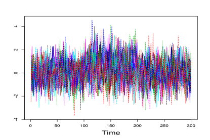
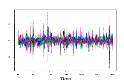
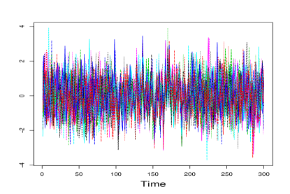
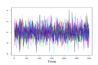
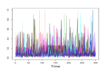
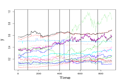
Figure 1: From left to right and from top to bottom, the first five plots illustrate raw data generated from Scenarios 1 to 5, respectively, with one realization each. In each case, $T=300$ and $p=20$, with the x-axis representing the time horizon, and the y-axis the values of each measurement. Different curves in each plot are associated with different coordinates of the vector $X(t)$. The right panel in the third row illustrates the raw data and estimated change points by MNP for the example in Section 4.2.

Scenario 1.

We generate data as

$$X(t)=\mu(t)+\epsilon(t),\quad t\in\{1,\ldots,T\},$$

where $\epsilon(t)\sim N(0,I_{p})$ and $I_{p}$ is the $p\times p$ identity matrix. Moreover, the mean vectors satisfy

$$\mu(t)=\begin{cases}v^{(0)}&t\in A_{1}\cup A_{3},\\ v^{(1)}&\text{otherwise,}\end{cases}$$

where $v^{(0)}=0\in\mathbb{R}^{p}$, and $v_{j}^{(1)}=1$ for $j\in\{1,\ldots,p/2\}$ and $v_{j}^{(1)}=0$ otherwise.

Scenario 2.

This is the same as Scenario 1 but with the errors satisfying $\sqrt{3}\,\epsilon(1),\ldots,\sqrt{3}\,\epsilon(T)\stackrel{{\scriptstyle\mbox{i.i.d.}}}{{\sim}}\mathrm{Mt}(I_{p},3)$, which is the multivariate $t$-distribution with the scale matrix $I_{p}$ and the degrees of freedom three. With respect to Scenario 1 we also change the value of $v^{(1)}$. This is now $v^{(1)}=0.1\cdot\boldsymbol{1}$ with $\boldsymbol{1}=(1,\ldots,1)^{\top}\in\mathbb{R}^{p}$.

Scenario 3.

We generate observations from the model

$$X(t)\stackrel{{\scriptstyle\mbox{i.i.d.}}}{{\sim}}N(0,\Sigma(t)),\quad t\in\{1,\ldots,T\},$$

where

$$\Sigma(t)=\begin{cases}I_{p}&t\in A_{1}\cup A_{3},\\ \frac{1}{2}I_{p}+\frac{1}{2}\boldsymbol{1}\boldsymbol{1}^{\top}&\text{otherwise.}\end{cases}$$

Scenario 4.

The observations are constructed as $X(t)\stackrel{{\scriptstyle\mbox{i.i.d.}}}{{\sim}}N(0,1.25I_{p})$ for $t\in A_{1}\cup A_{3}$, and for $t\in A_{2}$ we have

$$X(t)|\{u_{t}=1\}\stackrel{{\scriptstyle\mbox{i.i.d.}}}{{\sim}}N(0.5\cdot\boldsymbol{1},I_{p})\quad\mbox{and}\quad X(t)|\{u_{t}=2\}\stackrel{{\scriptstyle\mbox{i.i.d.}}}{{\sim}}N(-0.5\cdot\boldsymbol{1},I_{p}),$$

where the i.i.d. random variables $\{u_{t}\}$ satisfy $\mathbb{P}(u_{t}=1)=\mathbb{P}(u_{t}=2)=1/2$.

Scenario 5.

The vector $X(t)$ satisfies $X_{j}(t)\sim g_{1}$ for $t\in A_{1}\cap A_{3}$ and for all $j\in\{1,\ldots,p\}$. In contrast, if $t\in A_{2}$ we have that

$$X_{j}(t)\sim\begin{cases}g_{1},&j\in\{1,2\},\\ g_{2},&\text{otherwise.}\end{cases}$$

Here $g_{1}$ and $g_{2}$ are the densities shown in the left and right panels in Figure 2, respectively.

Figure 2: Densities taken from Padilla et al. (2018) and used in Scenario 5.

Table 1: Scenario 1.

Method	Metric	T = 300	T = 300	T = 150	T = 150
		p=20	p=10	p=20	p=10
MNP	$|K-\widehat{K}|$	0.0	0.0	0.0	0.0
EMNCP	$|K-\widehat{K}|$	0.1	0.0	0.0	0.0
KCPA	$|K-\widehat{K}|$	1.4	0.9	1.3	1.0
SBS	$|K-\widehat{K}|$	2.0	2.0	2.0	2.0
DCBS	$|K-\widehat{K}|$	0.0	0.0	0.0	0.1
MNP	$d(\widehat{\mathcal{C}}|\mathcal{C})$	1.0	2.0	1.0	2.0
EMNCP	$d(\widehat{\mathcal{C}}|\mathcal{C})$	0.0	1.0	0.0	0.0
KCPA	$d(\widehat{\mathcal{C}}|\mathcal{C})$	175.0	119.0	60.0	62.0
SBS	$d(\widehat{\mathcal{C}}|\mathcal{C})$	$\infty$	$\infty$	$\infty$	$\infty$
DCBS	$d(\widehat{\mathcal{C}}|\mathcal{C})$	1.0	1.0	1.0	3.0
MNP	$d(\mathcal{C}|\widehat{\mathcal{C}})$	1.0	2.0	1.0	2.0
EMNCP	$d(\mathcal{C}|\widehat{\mathcal{C}})$	0.0	1.0	0.0	0.0
KCPA	$d(\mathcal{C}|\widehat{\mathcal{C}})$	1.0	19	1.0	13.0
SBS	$d(\mathcal{C}|\widehat{\mathcal{C}})$	$-\infty$	$-\infty$	$-\infty$	$-\infty$
DCBS	$d(\mathcal{C}|\widehat{\mathcal{C}})$	1.0	1.0	1.0	3.0

Table 2: Scenario 2.

Method	Metric	T = 300	T = 300	T = 150	T = 150
		p=20	p=10	p=20	p=10
MNP	$|K-\widehat{K}|$	0.9	1.1	1.5	1.5
EMNCP	$|K-\widehat{K}|$	1.7	1.7	1.8	1.8
KCPA	$|K-\widehat{K}|$	1.04	1.0	1.0	1.4
SBS	$|K-\widehat{K}|$	2.0	2.0	2.0	2.0
DCBS	$|K-\widehat{K}|$	2.0	2.0	1.96	2.0
MNP	$d(\widehat{\mathcal{C}}|\mathcal{C})$	74.0	90	86.0	81.0
EMNCP	$d(\widehat{\mathcal{C}}|\mathcal{C})$	$\infty$	$\infty$	$\infty$	$\infty$
KCPA	$d(\widehat{\mathcal{C}}|\mathcal{C})$	126.0	133.0	51.0	86.0
SBS	$d(\widehat{\mathcal{C}}|\mathcal{C})$	$\infty$	$\infty$	$\infty$	$\infty$
DCBS	$d(\widehat{\mathcal{C}}|\mathcal{C})$	$\infty$	$\infty$	$\infty$	$\infty$
MNP	$d(\mathcal{C}|\widehat{\mathcal{C}})$	26.0	35.0	$-\infty$	1.0
EMNCP	$d(\mathcal{C}|\widehat{\mathcal{C}})$	$-\infty$	$-\infty$	$-\infty$	$-\infty$
KCPA	$d(\mathcal{C}|\widehat{\mathcal{C}})$	38.0	33.0	12.0	12.0
SBS	$d(\mathcal{C}|\widehat{\mathcal{C}})$	$-\infty$	$-\infty$	$-\infty$	$-\infty$
DCBS	$d(\mathcal{C}|\widehat{\mathcal{C}})$	$-\infty$	$-\infty$	$-\infty$	$-\infty$

Table 3: Scenario 3.

Method	Metric	T = 300	T = 300	T = 150	T = 150
		p=20	p=10	p=20	p=10
MNP	$|K-\widehat{K}|$	0.5	0.9	1.4	1.3
EMNCP	$|K-\widehat{K}|$	1.3	1.4	1.6	2.0
KCPA	$|K-\widehat{K}|$	1.2	0.9	1.0	1.1
SBS	$|K-\widehat{K}|$	2.0	2.0	2.0	2.0
DCBS	$|K-\widehat{K}|$	2.0	2.0	1.96	2.0
MNP	$d(\widehat{\mathcal{C}}|\mathcal{C})$	35.0	72.0	50.0	42.0
EMNCP	$d(\widehat{\mathcal{C}}|\mathcal{C})$	$\infty$	$\infty$	$\infty$	$\infty$
KCPA	$d(\widehat{\mathcal{C}}|\mathcal{C})$	97.0	102.0	50.0	51
SBS	$d(\widehat{\mathcal{C}}|\mathcal{C})$	$\infty$	$\infty$	$\infty$	$\infty$
DCBS	$d(\widehat{\mathcal{C}}|\mathcal{C})$	$\infty$	$\infty$	$\infty$	$\infty$
MNP	$d(\mathcal{C}|\widehat{\mathcal{C}})$	18.0	27.0	12.0	8.0
EMNCP	$d(\mathcal{C}|\widehat{\mathcal{C}})$	$-\infty$	$-\infty$	$-\infty$	$-\infty$
KCPA	$d(\mathcal{C}|\widehat{\mathcal{C}})$	6.0	6.0	2.0	10
SBS	$d(\mathcal{C}|\widehat{\mathcal{C}})$	$-\infty$	$-\infty$	$-\infty$	$-\infty$
DCBS	$d(\mathcal{C}|\widehat{\mathcal{C}})$	$-\infty$	$-\infty$	$-\infty$	$-\infty$

Table 4: Scenario 4.

Method	Metric	T = 300	T = 300	T = 150	T = 150
		p=20	p=10	p=20	p=10
MNP	$|K-\widehat{K}|$	0.7	0.9	1.1	1.4
EMNCP	$|K-\widehat{K}|$	1.8	1.8	2.0	1.8
KCPA	$|K-\widehat{K}|$	1.2	1.1	1.4	1.2
SBS	$|K-\widehat{K}|$	2.0	2.0	2.0	2.0
DCBS	$|K-\widehat{K}|$	2.0	2.0	1.9	2.0
MNP	$d(\widehat{\mathcal{C}}|\mathcal{C})$	38.0	68.0	43.0	65.0
EMNCP	$d(\widehat{\mathcal{C}}|\mathcal{C})$	$\infty$	$\infty$	$\infty$	$\infty$
KCPA	$d(\widehat{\mathcal{C}}|\mathcal{C})$	99.0	112.0	72.0	81.0
SBS	$d(\widehat{\mathcal{C}}|\mathcal{C})$	$\infty$	$\infty$	$\infty$	$\infty$
DCBS	$d(\widehat{\mathcal{C}}|\mathcal{C})$	$\infty$	$\infty$	$\infty$	$\infty$
MNP	$d(\mathcal{C}|\widehat{\mathcal{C}})$	36.0	33.0	7.0	6.0
EMNCP	$d(\mathcal{C}|\widehat{\mathcal{C}})$	$-\infty$	$-\infty$	$-\infty$	$\infty$
KCPA	$d(\mathcal{C}|\widehat{\mathcal{C}})$	3.0	34	1.0	22.0
SBS	$d(\mathcal{C}|\widehat{\mathcal{C}})$	$-\infty$	$-\infty$	$-\infty$	$-\infty$
DCBS	$d(\mathcal{C}|\widehat{\mathcal{C}})$	$-\infty$	$-\infty$	$-\infty$	$-\infty$

Table 5: Scenario 5.

Method	Metric	T = 300	T = 300	T = 150	T = 150
		p=20	p=10	p=20	p=10
MNP	$|K-\widehat{K}|$	0.8	0.8	1.7	1.2
EMNCP	$|K-\widehat{K}|$	1.6	0.6	1.9	1.4
KCPA	$|K-\widehat{K}|$	0.9	0.9	1.3	1.4
SBS	$|K-\widehat{K}|$	2.0	2.0	2.0	2.0
DCBS	$|K-\widehat{K}|$	1.8	1.9	2.0	2.0
MNP	$d(\widehat{\mathcal{C}}|\mathcal{C})$	41.0	45	$\infty$	53.0
EMNCP	$d(\widehat{\mathcal{C}}|\mathcal{C})$	$\infty$	12.0	$\infty$	$\infty$
KCPA	$d(\widehat{\mathcal{C}}|\mathcal{C})$	105.0	124.0	95.0	75.0
SBS	$d(\widehat{\mathcal{C}}|\mathcal{C})$	$\infty$	$\infty$	$\infty$	$\infty$
DCBS	$d(\widehat{\mathcal{C}}|\mathcal{C})$	$\infty$	$\infty$	$\infty$	$\infty$
MNP	$d(\mathcal{C}|\widehat{\mathcal{C}})$	35.0	42	$-\infty$	9.0
EMNCP	$d(\mathcal{C}|\widehat{\mathcal{C}})$	$-\infty$	7.0	$-\infty$	$-\infty$
KCPA	$d(\mathcal{C}|\widehat{\mathcal{C}})$	21.0	24.0	17.0	17.0
SBS	$d(\mathcal{C}|\widehat{\mathcal{C}})$	$-\infty$	$-\infty$	$-\infty$	$-\infty$
DCBS	$d(\mathcal{C}|\widehat{\mathcal{C}})$	$-\infty$	$-\infty$	$-\infty$	$-\infty$

Figure 1 illustrates examples of data generated from each of the scenarios that we consider. This is complemented by the results in Tables 1–5. Specifically, we observe that for Scenario 1, a setting with mean changes, the best methods seem to be MNP, DCBS and EMNCP.

Interestingly, from Table 2, we see that KCPA and MNP outperform the other methods. This setting presents a bigger challenge than Scenario 1, as it involves a heavy-tailed distribution of the errors and smaller changes in mean.

Scenario 3 posses a situation where the mean remains constant and the covariance structure changes. From Table 3, we observe that MNP and KCPA attain the best performance.

In Table 4, we also see the advantage of the MNP method which is the best at estimating the number of change points. This is in the context of Scenario 4 where the mean and covariance remain unchanged and the jumps happen in the shape of the distribution.

Finally, Scenario 5 is an example of a model that does not belong to a usual parametric family. In such setting, Table 5 shows that MNP, KCPA and EMNCP seem to provide better estimation of the number of change points and their locations as compared to the other two methods.

Overall, we can see that SBS and DCBS, these two methods designed for mean change point detection, are not robust in the cases where the changes are not mean or the noise is not sub-Gaussian. MNP and KCPA are, arguably, the best performing methods. KCPA is competitive and sometimes outperforms MNP.

4.2 Real data example

The experiments section concludes with an example using financial data. Specifically, our data consist of the daily close stock price, from Jan-1-2016 to Aug-11-2019, of the 20 companies with highest average stock price from the S&P500 market. The data can be downloaded from Microsoft Corp. (2019) (MSFT). Our final dataset is then a matrix $X\in\mathbb{R}^{T\times p}$, with $T=907$ and $p=20$.

We then run both the MNP procedure and the estimator from Matteson and James (2014). The implementation and details are the same as those in Section 4.1. Our goal is to detect potential change points in the period aforementioned and determine if they might have a financial meaning.

We find that our estimator localizes change points at the dates May-17-2016, March-2-2017, August-7-2017, December-21-2017, June-1-2018 and January-24-2019. The first change point seems to correspond with the moment when President Donald Trump, while still a presidential candidate, outlined his plan for the USA vs. China trade war (see e.g. Burns et al., 2019). The second change point, February-21-2017, might be associated with Trump signing two executive orders increasing tariffs on the trade with China; the date August-7-2017 could correspond to the bipartite agreement on July-19 2017 to reduce USA deficit with China; the date December-21-2017 could be explained by the threats and tariffs imposed by Trump to China in January of 2018. The other two dates are also relatively close to important dates in the USA vs. China trade war time-line. The raw data, scaled to the interval $[0,1]$, and the estimated change points can be seen in the right panel in the third row in Figure 1.

As for EMNCP, we find a total of 22 change points with spacings between 30 and 58 units of time. This might suggest that some of the change point are spurious as the minimum spacing parameter of the function e.divisive() is by default set to 30.

Finally, we also considered comparing with KCPA. However, the elbow could not be used as the scores produced by the function KernSeg_MultiD did not have an inflection point.

Appendix A Large probability events

In this section, we deal with all the large probability events occurred in the proof of Theorem 1. Lemma 4 is almost identical to Theorem 2.1 in Bousquet (2002) and therefore we omit the proof. Lemma 5 is an adaptation of Theorem 2.3 in Bousquet (2002) and Proposition 8 in Kim et al. (2018), but we allow for non-i.i.d. cases. Lemma 6 is a non-i.i.d. version of Proposition 2.1 in Giné and Guillou (2001). Lemma 7 is to control the deviance between the sample and population quantities and provides an lower bound on a large probability event. Lemma 8 is to provide a lower bound on the probability of the event that the data can reach the maxima closely enough. Lemma 9 is identical to Lemma 13 in Wang et al. (2018b), controlling the random intervals selected in Algorithm 1.

Lemma 4.

Let $\mathcal{D}$ be the $\sigma$-field generated by $\{X(i)\}_{i=1}^{T}$, $\mathcal{D}^{t}_{T}$ be the $\sigma$-field generated by $\{X(i)\}_{i=1}^{T}\setminus\{X(t)\}$ and $\mathbb{E}^{t}_{T}(\cdot)$ be the conditional expectation given $\mathcal{D}_{T}^{t}$, for all $t\in\{1,\ldots,T\}$. Let $(Z,Z_{1}^{\prime},\ldots,Z_{T}^{\prime})$ be a sequence of $\mathcal{D}$-measurable random variables, and $\{Z_{k}\}_{k=1}^{T}$ be a sequence of random variables such that $Z_{k}$ measurable with respect to $\mathcal{D}_{T}^{k}$, for all $k$. Assume that there exists $u>0$ such that for all $k=1,\ldots,T$, the following inequalities hold

$$Z_{k}^{\prime}\leq Z-Z_{k}\,\mbox{a.s.},\quad\mathbb{E}_{T}^{k}(Z_{k}^{\prime})\geq 0\quad\mbox{and}\quad Z_{k}^{\prime}\leq u\quad\mbox{a.s.}.$$ (15)

Let $\sigma$ be a real value satisfying $\sigma^{2}\geq\sum_{k=1}^{T}\mathbb{E}^{k}_{T}\{(Z_{k}^{\prime})^{2}\}$ almost surely and let $\nu=(1+u)\mathbb{E}(Z)+\sigma^{2}$. If

$$\sum_{k=1}^{T}(Z-Z_{k})\leq Z\quad\mbox{a.s.},$$ (16)

then for all $x>0$,

$$\mathbb{P}\bigl{\{}Z\geq\mathbb{E}(Z)+\sqrt{2\nu x}+x/3\bigr{\}}\leq e^{-x}.$$

Lemma 5.

Assume that $\{X(i)\}_{i=1}^{T}$ satisfy 1. Let $\mathcal{F}$ be a class of functions from $\mathbb{R}^{p}$ to $\mathbb{R}$ that is separable in $L_{\infty}(\mathbb{R}^{p})$. Suppose all functions $g\in\mathcal{F}$ are measurable with respect to $P_{\eta_{k}}$, $k\in\{1,\ldots,K+1\}$, and there exist $B,\sigma>0$ such that for all $g\in\mathcal{F}$

$$\mathbb{E}_{P_{\eta_{k}}}\{g^{2}\}-(\mathbb{E}_{P_{\eta_{k}}}\{g\})^{2}\leq\sigma^{2}\quad\mbox{and}\quad\|g\|_{\infty}\leq B.$$

Let $Z=\sup_{g\in\mathcal{F}}\big{|}\sum_{i=1}^{T}w_{i}[g(X(i))-\mathbb{E}_{P_{i}}\{g(X(i))\}]\big{|}$, with $\sum_{i=1}^{T}w_{i}^{2}=1$ and $\max_{i=1,\ldots,T}|w_{i}|=w$. Then for any $\varepsilon>0$ , we have

$$\mathbb{P}\left\{Z\geq\mathbb{E}(Z)+\sqrt{2\{(1+wB)\mathbb{E}(Z)+\sigma^{2}\}x}+x/3\right\}\leq e^{-x}.$$

Proof.

For all $k\in\{1,\ldots,T\}$, define

$$Z_{k}=\sup_{g\in\mathcal{F}}\left|\sum_{i\neq k}w_{i}[g(X(i))-\mathbb{E}_{P_{i}}\{g(X(i))\}]\right|$$

and

$$Z_{k}^{\prime}=\left|\sum_{i=1}^{T}w_{i}[g_{k}(X(i))-\mathbb{E}_{P_{i}}\{g_{k}(X(i))\}]\right|-Z_{k},$$

where $g_{k}$ denotes the function for which the supremum is obtained in $Z_{k}$. We then have

$$Z_{k}^{\prime}\leq Z-Z_{k} \leq\left|\sum_{i=1}^{T}w_{i}[g_{0}(X(i))-\mathbb{E}_{P_{i}}\{g_{0}(X(i))\}]\right|-\left|\sum_{i\neq k}w_{i}[g_{0}(X(i))-\mathbb{E}_{P_{i}}\{g_{0}(X(i))\}]\right|$$

$$\leq|w_{k}[g_{0}(X(k))-\mathbb{E}_{P_{k}}\{g_{0}(X(k))\}]|\leq wB\quad\mbox{a.s.},$$

where $g_{0}$ is the function for which the supremum is obtained in $Z$. Moreover, we have

$$\mathbb{E}^{k}_{T}(Z_{k}^{\prime})\geq\left|\sum_{i=1}^{T}\mathbb{E}_{T}^{k}\{w_{i}(g_{k}(X(i))-\mathbb{E}_{P_{i}}\{g_{k}(X(i))\})\}\right|-Z_{k}=0,$$

which concludes the proof of (15) with $u=B$. In addition,

$$(T-1)Z =\left|\sum_{k=1}^{T}\sum_{i\neq k}w_{i}[g_{0}(X(i))-\mathbb{E}_{P_{i}}\{g_{k}(X(i))\}]\right|$$

$$\leq\sum_{k=1}^{T}\left|\sum_{i\neq k}w_{i}[g_{0}(X(i))-\mathbb{E}_{P_{i}}\{g_{k}(X(i))\}]\right|\leq\sum_{k=1}^{T}Z_{k},$$

which leads to (16). Finally, since

$$\sum_{k=1}^{T}\mathbb{E}_{T}^{k}\bigl{\{}(Z_{k}^{\prime})^{2}\bigr{\}}\leq\sum_{k=1}^{T}\mathrm{Var}_{T}^{k}\bigl{\{}w_{k}g_{k}(X(k))\bigr{\}}\leq\max_{k}\sup_{g}\mathrm{Var}\{g(X(k))\}\leq\sigma^{2},$$

it follows due to Lemma 4 that

$$\mathbb{P}\left\{Z\geq\mathbb{E}(Z)+\sqrt{2\{(1+wB)\mathbb{E}(Z)+\sigma^{2}\}x}+x/3\right\}\leq e^{-x},$$

for all $x>0$. ∎

Lemma 6.

Let $\mathcal{F}$ be a uniformly bounded VC class of functions, and measurable with respect to all $P_{\eta_{k}}$, $k=1,\ldots,K+1$. Suppose

$$\sup_{g\in\mathcal{F}}\mathrm{Var}_{P_{\eta_{k}}}(g)\leq\sigma^{2},\quad\sup_{g\in\mathcal{F}}\|g\|_{\infty}\leq B,\quad\mbox{and}\quad 0<\sigma\leq B.$$

Then there exist positive constants $A$ and $\nu$ depending on $\mathcal{F}$ but not on $\{P_{\eta_{k}}\}_{k=1}^{K+1}$ or $T$, such that for all $T\in\mathbb{N}$,

$$\sup_{g\in\mathcal{F}}\mathbb{E}\left\|\sum_{i=1}^{T}w_{i}\{g(X_{i})-\mathbb{E}(g(X_{i}))\}\right\|\leq C\left\{\nu wB\log(2AwB/\sigma)+\sqrt{\nu}\sigma\sqrt{\log(2AwB/\sigma)}\right\},$$

where $C$ is a universal constant, $\sum_{i=1}^{T}w_{i}^{2}=1$ and $\max_{i=1,\ldots,T}|w_{i}|=w$.

The proof of Lemma 6 is almost identical to that of Propostion 2.1 in Giné and Guillou (2001), except noticing that $\sum_{i=1}^{T}w_{i}^{2}=1$.

For any $x\in\mathbb{R}^{p}$, $0\leq s<t<e\leq T$ and $h>0$, define

$$\widetilde{f}^{s,e}_{t,h}(x)=\sqrt{\frac{e-t}{(e-s)(t-s)}}\sum_{j=s+1}^{t}f_{j,h}(x)-\sqrt{\frac{t-s}{(e-s)(e-t)}}\sum_{j=t+1}^{e}f_{j,h}(x),$$ (17)

where

$$f_{j,h}(x)=h^{-p}\mathbb{E}\left\{\mathpzc{k}\left(\frac{x-X(j)}{h}\right)\right\}$$

and the expectation is taken with respect to the distribution $P_{j}$.

Lemma 7.

Define the events

$$\mathcal{A}_{1}(\gamma,h)=\left\{\max_{0\leq s<t-h^{-p}<t+h^{-p}<e\leq T}\,\sup_{z\in\mathbb{R}^{p}}\,\left|\widetilde{Y}^{s,e}_{t}(z)-\widetilde{f}^{s,e}_{t,h}(z)\right|\leq\gamma\right\}$$

and

$$\mathcal{A}_{2}(\gamma,h)=\Bigg{\{}\max_{0\leq s<t-h^{-p}<t+h^{-p}<e\leq T}\,\sup_{z\in\mathbb{R}^{p}}\frac{1}{\sqrt{e-s}}\Bigg{|}\sum_{j=s+1}^{e}\left(\hat{f}_{j,h}(z)-f_{j,h}(z)\right)\Bigg{|}\leq\gamma\Bigg{\}}.$$

Under Assumptions 1 and 2, we have that

$$\mathbb{P}\left\{\mathcal{A}_{1}\left(Ch^{-p/2}\sqrt{\log(T)},h\right)\right\}\geq 1-T^{-c}$$

and

$$\mathbb{P}\left\{\mathcal{A}_{2}\left(Ch^{-p/2}\sqrt{\log(T)},h\right)\right\}\geq 1-T^{-c},$$

where $C,c>0$ are absolute constants depending on $\|\mathpzc{k}\|_{\infty}$, $A$ and $\nu$.

We remark that the proof here is an adaptation of Theorem 12 in Kim et al. (2018).

Proof.

For any fixed $x\in\mathbb{R}^{p}$, it holds that

$$\widetilde{Y}^{s,e}_{t}(x)-\widetilde{f}^{s,e}_{t,h}(x)=\sum_{j=s+1}^{e}w_{j}\left[h^{-p}\mathpzc{k}\left(\frac{x-X(j)}{h}\right)-\mathbb{E}\left\{h^{-p}\mathpzc{k}\left(\frac{x-X(j)}{h}\right)\right\}\right],$$ (18)

where

$$w_{j}=\begin{cases}\sqrt{\frac{e-t}{(e-s)(t-s)}},&j=s+1,\ldots,t,\\ -\sqrt{\frac{t-s}{(e-s)(e-t)}},&j=t+1,\ldots,e,\end{cases}$$

satisfying that

$$\sum_{j=s+1}^{e}w_{j}^{2}=1\quad\mbox{and}\quad\max_{j=s+1,\ldots,e}|w_{j}|\leq h^{p/2}.$$

Step 1. Let $\mathpzc{K}_{x,h}:\,\mathbb{R}^{p}\to\mathbb{R}$ be $\mathpzc{K}_{x,h}(\cdot)=\mathpzc{k}(h^{-1}x-h^{-1}\cdot)$ and

$$\widetilde{\mathcal{F}}_{\mathpzc{k},h}=\{h^{-p}\mathpzc{K}_{x,h}:\,x\in\mathcal{X}\}$$

be a class of normalized kernel functions centred on $\mathcal{X}$ and bandwidth $h$. It follows from (18) that, for each $s,t,e$,

$$\sup_{x\in\mathcal{X}}\bigl{|}\widetilde{Y}^{s,e}_{t}(x)-\widetilde{f}^{s,e}_{t,h}(x)\bigr{|}=\sup_{g\in\widetilde{\mathcal{F}}_{\mathpzc{k},h}}\left|\sum_{j=s+1}^{e}w_{j}\bigl{[}g(X(j))-\mathbb{E}\{g(X(j))\}\bigr{]}\right|=W_{s,t,e}.$$

It is immediate to check that for any $g\in\widetilde{\mathcal{F}}_{\mathpzc{k},h}$,

$$\|g\|_{\infty}\leq h^{-p}\|\mathpzc{k}\|_{\infty}.$$

Due to the arguments used in Theorem 12 in Kim et al. (2018) and 2 (i), for every probability measure $Q$ on $\mathbb{R}^{p}$ and for every $\zeta\in(0,h^{-p}\|\mathpzc{k}\|_{\infty})$, the covering number $\mathcal{N}(\widetilde{F}_{\mathpzc{k},h},L_{2}(Q),\zeta)$ is upper bounded as

$$\sup_{Q}\mathcal{N}(\widetilde{F}_{\mathpzc{k},h},L_{2}(Q),\zeta)\leq\left(\frac{2Ap\|\mathpzc{k}\|_{\infty}}{h^{p}\zeta}\right)^{\nu+2}.$$

Under 2, due to Lemma 11 in Kim et al. (2018), it holds that for any $j=1,\ldots,T$,

$$\mathbb{E}\left\{\left(h^{-p}\mathpzc{K}_{x,h}(X(j))\right)^{2}\right\}\leq C_{1}h^{-p},$$

where $C_{1}$ is an absolute constant.

It follows from Lemma 5 that for any $x>0$,

$$\mathbb{P}\left\{W_{s,t,e}<\mathbb{E}(W_{s,t,e})+\sqrt{2\{(1+h^{-p/2}\|\mathpzc{k}\|_{\infty})\mathbb{E}(W_{s,t,e})+C_{1}h^{-p}\}x}+x/3\right\}\geq 1-e^{-x}.$$ (19)

Step 2. We then need to bound $\mathbb{E}(W_{s,t,e})$, where the expectation is taken on the product of $P_{1}\otimes\ldots\otimes P_{T}$. Let $\check{\mathcal{F}}=\{g-a:\,g\in\widetilde{\mathcal{F}}_{\mathpzc{k},h},a\in[-h^{-p}\|\mathpzc{k}\|_{\infty},h^{-p}\|\mathpzc{k}\|_{\infty}]\}$. Then for any $a\in[-h^{-p}\|\mathpzc{k}\|_{\infty},h^{-p}\|\mathpzc{k}\|_{\infty}]$, it follows from the proof of Theorem 30 in Kim et al. (2018) that

$$\sup_{P}\mathcal{N}(\check{\mathcal{F}},L_{2}(P),a)\leq(2Ah^{-p}\|\mathpzc{k}\|_{\infty}/a)^{\nu+1}.$$

Applying Lemma 6, we have

$$\mathbb{E}(W_{s,t,e})\leq C\left\{(\nu+1)\frac{\|\mathpzc{k}\|_{\infty}}{h^{p/2}}\log\left(\frac{8Ah^{-p/2}\|\mathpzc{k}\|_{\infty}}{C_{1}^{1/2}h^{-p/2}}\right)+h^{-p/2}\sqrt{(\nu+1)\log\left(\frac{8Ah^{-p/2}\|\mathpzc{k}\|_{\infty}}{C_{1}^{1/2}h^{-p/2}}\right)}\right\}.$$ (20)

Step 3. We now plug (20) into (19) and take $x=\log(T^{m})$, with $m>4$, resulting in

$$\mathbb{P}\left\{W_{s,t,e}<C_{2}h^{-p/2}\log^{1/2}(T)\right\}\geq 1-C_{3}T^{-m},$$

where $C_{2},C_{3}>0$ are absolute constants depending on $\|\mathpzc{k}\|_{\infty}$, $A$ and $\nu$. The final claims follow with a union bound argument over $s,t,e$.

∎

Lemma 8.

Under Assumptions 1, 2 and 3, for $s<t<e$, define

$$z^{*}_{s,e,t}\in\operatorname*{arg\,max}_{z\in\mathbb{R}^{p}}\left|\widetilde{f}^{s,e}_{t}(z)\right|.$$

With $h=c_{h}\kappa$, define the event

$$\mathcal{B}(\gamma)=\left\{\max_{\stackrel{{\scriptstyle 0\leq s<t<e\leq T}}{{e-s\leq C_{R}\Delta}}}\left|\max_{j=1,\ldots,T}\left|\widetilde{f}^{s,e}_{t,h}(X(j))\right|-\left|\widetilde{f}^{s,e}_{t,h}(z^{*}_{s,e,t})\right|\right|\leq\gamma,\,(s,e)\mbox{satisfies Condition }\mathpzc{SE}\right\},$$

where Condition $\mathpzc{SE}$ is defined as follows: the interval $(s,e)$ is such that either

• there is no true change point in $(s,e)$; or

• there exists at least one true change point in $\eta_{k}\in(s,e)$ satisfying

  $$\min\left\{\min_{\eta_{k}>s}\{\eta_{k}-s\},\,\min_{\eta_{k}<e}\{e-\eta_{k}\}\right\}>c_{1}\Delta,$$

  for some $c_{1}>0$;

• there exists one and only one change point $\eta_{k}\in(s,e)$ satisfying

  $$\min\{\eta_{k}-s,\,e-\eta_{k}\}\leq C_{\epsilon}\log(T)V_{p}^{2}\kappa^{-p}\kappa_{k}^{-2};$$

  or

• there exist exactly two change points $\eta_{k},\eta_{k+1}\in(s,e)$ with $\eta_{k}<\eta_{k+1}$ satisfying

  $$\eta_{k}-s\leq C_{\epsilon}\log(T)V_{p}^{2}\kappa^{-p}\kappa_{k}^{-2},\quad\mbox{and}\quad e-\eta_{k+1}\leq C_{\epsilon}\log(T)V_{p}^{2}\kappa^{-p}\kappa_{k}^{-2}.$$

Then for

$$\gamma=C_{\gamma}h\sqrt{\Delta},$$ (21)

with

$$C_{\gamma}>2C_{\mathrm{Lip}}\sqrt{C_{R}},$$ (22)

it holds that

$$\mathbb{P}\left\{\mathcal{B}(\gamma)\right\}\geq 1-T^{3}\exp\left\{-\frac{\Delta}{8}\left(\frac{c\gamma}{4\sqrt{C_{R}\Delta}C_{\mathrm{Lip}}}\right)^{p+1}V_{p}\right\},$$

for some constant $c>0$.

Proof.

Fix $0\leq s<t<e\leq T$ with $e-s\leq C_{R}\Delta$.

For case (a), it holds that $\widetilde{f}^{s,e}_{t,h}(x)=0$, for all $x\in\mathbb{R}^{p}$, and the claim holds consequently.

For case (b), if $\left|\widetilde{f}^{s,e}_{t,h}(z^{*}_{s,e,t})\right|<\gamma$, then by the definition of $z^{*}_{s,e,t}$, we have that

$$\left|\max_{j=1,\ldots,T}\left|\widetilde{f}^{s,e}_{t,h}(X(j))\right|-\left|\widetilde{f}^{s,e}_{t,h}(z^{*}_{s,e,t})\right|\right|=\left|\widetilde{f}^{s,e}_{t,h}(z^{*}_{s,e,t})\right|-\max_{j=1,\ldots,T}\left|\widetilde{f}^{s,e}_{t,h}(X(j))\right|\leq\left|\widetilde{f}^{s,e}_{t,h}(z^{*}_{s,e,t})\right|<\gamma,$$

which implies that

$$\mathbb{P}\left\{\left|\underset{j=1,\ldots,T}{\max}\left|\widetilde{f}^{s,e}_{t,h}(X(j))\right|-\left|\widetilde{f}^{s,e}_{t,h}(z^{*}_{s,e,t})\right|\right|>\gamma\right\}=0.$$ (23)

If $\left|\widetilde{f}^{s,e}_{t,h}(z^{*}_{s,e,t})\right|>\gamma$, then

$$\gamma<\left|\widetilde{f}^{s,e}_{t,h}(z^{*}_{s,e,t})\right|\leq 2\min\bigl{\{}\sqrt{t-s},\,\sqrt{e-t}\bigr{\}}\underset{j=1,\ldots,T}{\max}|f_{j,h}(z^{*}_{s,e,t})|,$$ (24)

there exists $j_{0}\in\{1,\ldots,K+1\}$ such that

$$f_{\eta_{j_{0}}}(z^{*}_{s,e,t}) \geq f_{\eta_{j_{0}},h}(z^{*}_{s,e,t})-C_{\mathrm{Lip}}h\geq\frac{\gamma}{2\min\bigl{\{}\sqrt{t-s},\,\sqrt{e-t}\bigr{\}}}-C_{\mathrm{Lip}}h$$

$$\geq\frac{c\gamma}{2\min\bigl{\{}\sqrt{t-s},\,\sqrt{e-t}\bigr{\}}},$$ (25)

where $0<c<1$ is an absolute constant, the first inequality follows from (B), the second inequality follows from (24), and the last inequality follows from 3 and the choice of $\gamma$.

As for the function $\widetilde{f}^{s,e}_{t,h}(\cdot)$, for any $x_{1},x_{2}\in\mathbb{R}^{p}$, it holds that

$$\left|\widetilde{f}^{s,e}_{t,h}(x_{1})-\widetilde{f}^{s,e}_{t,h}(x_{2})\right| =\Bigg{|}\sqrt{\frac{e-t}{(e-s)(t-s)}}\sum_{j=s+1}^{t}\int_{\mathbb{R}^{p}}\mathpzc{k}(y)\left\{f_{j}(x_{1}-hy)-f_{j}(x_{2}-hy)\right\}\,dy$$

$$-\sqrt{\frac{t-s}{(e-s)(e-t)}}\sum_{j=t+1}^{e}\int_{\mathbb{R}^{p}}\mathpzc{k}(y)\left\{f_{j}(x_{1}-hy)-f_{j}(x_{2}-hy)\right\}\,dy\Bigg{|}$$

$$\leq 2\min\{\sqrt{e-t},\,\sqrt{t-s}\}C_{\mathrm{Lip}}\|x_{1}-x_{2}\|,$$ (26)

where the last inequality follows from Assumption 1. As a result, the function $\widetilde{f}^{s,e}_{t,h}(\cdot)$ is Lipschitz with constant $2\min\{\sqrt{e-t},\,\sqrt{t-s}\}C_{\mathrm{Lip}}$. Furthermore, defining

$$d_{j_{0}}=\left|\left\{j\in\{\eta_{j_{0}-1}+1,\ldots,\eta_{j_{0}}\}:\,\|X(j)-z_{s,e,t}^{*}\|\,\leq\,\frac{\gamma}{2\min\{\sqrt{t-s},\sqrt{e-t}\}C_{\mathrm{Lip}}}\right\}\right|,$$

and noticing that

$$d_{j_{0}}\sim\text{Binomial}\left(\eta_{j_{0}+1}-\eta_{j_{0}},\int_{B(z_{s,e,t}^{*},\frac{\gamma}{2\min\{\sqrt{t-s},\sqrt{e-t}\}C_{\mathrm{Lip}}})}f_{\eta_{j_{0}}}(z)\,dz\right),$$

we arrive at

$$\mathbb{P}\left\{\left|\underset{j=1,\ldots,T}{\max}\left|\widetilde{f}^{s,e}_{t,h}(X(j))\right|-\left|\widetilde{f}^{s,e}_{t,h}(z^{*}_{s,e,t})\right|\right|>\gamma\right\}=\mathbb{P}\left\{\underset{j=1,\ldots,T}{\min}\left|\widetilde{f}^{s,e}_{t,h}(X(j))-\widetilde{f}^{s,e}_{t}(z^{*}_{s,e,t})\right|>\gamma\right\}$$

$$\leq \mathbb{P}\left\{\underset{j=1,\ldots,T}{\min}\left\|X(j)-z^{*}_{s,e,t}\right\|>\frac{\gamma}{2\min\{\sqrt{e-t},\,\sqrt{t-s}\}C_{\mathrm{Lip}}}\right\}\leq\mathbb{P}\{d_{j_{0}}=0\},$$ (27)

where the identity follows from the definition of $z_{s,e,t}^{*}$, the first inequality follows from (26) and the second inequality follows from the definition of $d_{j_{0}}$.

In addition, we have that

$$\int_{B\left(z_{s,e,t}^{*},\,\frac{\gamma}{2\min\{\sqrt{t-s},\,\sqrt{e-t}\}C_{\mathrm{Lip}}}\right)}f_{\eta_{j_{0}}}(z)\,dz\geq\int_{B\left(z_{s,e,t}^{*},\,\frac{c\gamma}{4\min\{\sqrt{t-s},\,\sqrt{e-t}\}C_{\mathrm{Lip}}}\right)}f_{\eta_{j_{0}}}(z)\,dz$$

$$\geq \int_{B\left(z_{s,e,t}^{*},\,\frac{c\gamma}{4\min\{\sqrt{t-s},\,\sqrt{e-t}\}C_{\mathrm{Lip}}}\right)}\left\{f_{\eta_{j_{0}}}(z^{*}_{s,e,t})-\frac{c\gamma}{4\min\{\sqrt{t-s},\,\sqrt{e-t}\}C_{\mathrm{Lip}}}\right\}\,dz$$

$$\geq \left(\frac{c\gamma}{4\min\{\sqrt{t-s},\,\sqrt{e-t}\}C_{\mathrm{Lip}}}\right)^{p+1}V_{p},$$ (28)

where the last inequality is due to (25). Therefore,

$$\mathbb{P}\{d_{j_{0}}=0\} \leq\mathbb{P}\left\{d_{j_{0}}\leq\frac{\Delta}{2}\left(\frac{c\gamma}{4\min\{\sqrt{t-s},\,\sqrt{e-t}\}C_{\mathrm{Lip}}}\right)^{p+1}V_{p}\right\}$$

$$\leq\mathbb{P}\left\{d_{j_{0}}\leq\frac{(\eta_{j_{0}}-\eta_{j_{0}-1})}{2}\int_{B\left(z_{s,e,t}^{*},\,\frac{\gamma}{2\min\{\sqrt{t-s},\,\sqrt{e-t}\}C_{\mathrm{Lip}}}\right)}f_{\eta_{j_{0}}}(z)\,dz\right\}$$

$$\leq\exp\left\{-\frac{(\eta_{j_{0}}-\eta_{j_{0}-1})}{8}\int_{B\left(z_{s,e,t}^{*},\,\frac{\gamma}{2\min\{\sqrt{t-s},\,\sqrt{e-t}\}C_{\mathrm{Lip}}}\right)}f_{\eta_{j_{0}}}(z)\,dz\right\}$$

$$\leq\exp\left\{-\frac{\Delta}{8}\left(\frac{c\gamma}{4\sqrt{C_{R}\Delta}C_{\mathrm{Lip}}}\right)^{p+1}V_{p}\right\},$$ (29)

where the second and the fourth inequality follow from (28), and the third by the Chernoff bound (e.g. Mitzenmacher and Upfal, 2017). Combining (23), (27) and (29) results in

$$\mathbb{P}\left\{\left|\underset{j=1,\ldots,T}{\max}\left|\widetilde{f}^{s,e}_{t,h}(X(j))\right|-\left|\widetilde{f}^{s,e}_{t,h}(z^{*}_{s,e,t})\right|\right|>\gamma\right\}\leq\exp\left\{-\frac{\Delta}{8}\left(\frac{c\gamma}{4\sqrt{C_{R}\Delta}C_{\mathrm{Lip}}}\right)^{p+1}V_{p}\right\}.$$

The conclusion follows from a union bound.

Cases (c) and (d) are similar, and we only deal with case (c) here. Note that

$$\left|\widetilde{f}^{s,e}_{t}(z^{*}_{s,e,t})\right|\leq\kappa_{k}\sqrt{C_{\epsilon}\log(T)V_{p}^{2}\kappa_{k}^{-2}\kappa^{-p}}\leq\gamma,$$ (30)

where the first inequality follows from Lemma 13 (i) and the second follows from 3. The final claim holds due to the fact that $\widetilde{f}^{s,e}_{t,h}$ is a smoothed version of $\widetilde{f}^{s,e}_{t}$. ∎

We independently select at random from $\{1,\ldots,T\}$ two sequences $\{\alpha_{m}\}_{m=1}^{M_{1}},\{\beta_{m}\}_{m=1}^{M_{1}}$, then we keep the pairs which satisfy $\beta_{m}-\alpha_{m}\leq C_{R}\Delta$, with $C_{R}\geq 3/2$. For notational simplicity, we label them as $\{\alpha_{m}\}_{m=1}^{R},\{\beta_{m}\}_{m=1}^{R}$. Let

$$\mathcal{M}=\bigcap_{k=1}^{K}\bigl{\{}\alpha_{m}\in\mathcal{S}_{k},\beta_{m}\in\mathcal{E}_{k},\,\mbox{for some }m\in\{1,\ldots,R\}\bigr{\}},$$ (31)

where $\mathcal{S}_{k}=[\eta_{k}-3\Delta/4,\eta_{k}-\Delta/2]$ and $\mathcal{E}_{k}=[\eta_{k}+\Delta/2,\eta_{k}+3\Delta/4]$, $k=1,\ldots,K$. In the lemma below, we give a lower bound on the probability of $\mathcal{M}$.

Lemma 9.

For the event $\mathcal{M}$ defined in (31), we have

$$\mathbb{P}(\mathcal{M})\geq 1-\exp\left\{\log\left(\frac{T}{\Delta}\right)-\frac{R\Delta}{4C_{R}T}\right\}.$$

See Lemma S.24 in Wang et al. (2018a) for the proof of Lemma 9.

Appendix B Change point detection lemmas and the proof of Theorem 1

Lemma 10 below provides a lower bound on the maximum of the population CUSUM statistic when there exists a true change point. Lemma 11 shows that the maxima of the population CUSUM statistic are the true change points. Lemma 13 is a collection of results on the population quantities. Lemma 14 provides an initial upper bound for the localization error. Lemma 15 is the key lemma to provide the final localization rate. The proof of Theorem 1 is collected at the end of this section.

In the rest of this section, we will adopt the notation

$$\widetilde{f}^{s,e}_{t}(x)=\sqrt{\frac{e-t}{(e-s)(t-s)}}\sum_{j=s+1}^{t}f_{j}(x)-\sqrt{\frac{t-s}{(e-s)(e-t)}}\sum_{j=t+1}^{e}f_{j}(x),$$

for all $0\leq s<t<e\leq T$ and $x\in\mathbb{R}^{p}$.

Lemma 10.

Under Assumptions  1-3, let $(s,e)$ be an interval such that $e-s\leq C_{R}\Delta$ and there exists a true change point $\eta_{k}\in(s,e)$ with

$$\min\{\eta_{k}-s,\,e-\eta_{k}\}>c_{1}\Delta,$$

where $c_{1}>0$ is a large enough constant, depending on all the other absolute constants. Then for any $h$ such that

$$(\log(T)/\Delta)^{1/p}\leq h\leq\frac{c_{1}}{C_{R}C_{\mathrm{Lip}}C_{\mathpzc{k}}}\kappa,$$ (32)

it holds that

$$\max_{s+h^{-p}<t<e-h^{-p}}\sup_{z\in\mathbb{R}^{p}}\left|\widetilde{f}^{s,e}_{t,h}(z)\right|\geq\frac{c_{1}\kappa\Delta}{4\sqrt{e-s}}.$$

Proof.

Let $z_{1}\in\operatorname*{arg\,max}_{z\in\mathbb{R}^{p}}\bigl{|}f_{\eta_{k}}(z)-f_{\eta_{k+1}}(z)\bigr{|}$. Due to Assumption 1, we have that

$$\bigl{|}f_{\eta_{k}}(z_{1})-f_{\eta_{k+1}}(z_{1})\bigr{|}\geq\kappa_{k}\geq\kappa.$$

Then by the argument in Lemma 2.4 of Venkatraman (1992), we have that

$$\max_{t\in\{\eta_{k}+c_{1}\Delta/2,\eta_{k}-c_{1}\Delta/2\}}\left|\widetilde{f}^{s,e}_{t}(z_{1})\right|\geq\frac{c_{1}\kappa\Delta}{2\sqrt{e-s}}.$$ (33)

Next, for any $x\in\mathbb{R}^{p}$, $h>0$ and $j\in\{1,\ldots,T\}$, we have

$$\bigl{|}f_{j}(x)-f_{j,h}(x)\bigr{|} =\left|\int_{\mathbb{R}^{p}}\frac{1}{h^{p}}\mathpzc{k}(y/h)\{f_{j}(x-y)-f_{j}(x)\}\,dy\right|\leq\frac{C_{\mathrm{Lip}}}{h^{p}}\int_{\mathbb{R}^{p}}\mathpzc{k}(y/h)\|y\|\,dy$$

$$\leq hC_{\mathrm{Lip}}\int_{\mathbb{R}^{p}}\mathpzc{k}(z)\|z\|\,dz\leq C_{\mathrm{Lip}}C_{\mathpzc{k}}h,$$ (34)

where the last inequality follows from 2 (iii). Hence, for $t\in\{\eta_{k}+c_{1}\Delta/2,\eta_{k}-c_{1}\Delta/2\}$

$$\left|\widetilde{f}^{s,e}_{t,h}(z_{1})-\widetilde{f}^{s,e}_{t}(z_{1})\right|\leq C_{\mathrm{Lip}}C_{\mathpzc{k}}h\sqrt{\frac{(e-t)(t-s)}{e-s}}\leq\sqrt{(e-s)}C_{\mathrm{Lip}}C_{\mathpzc{k}}h\leq\frac{c_{1}\kappa\Delta}{4\sqrt{e-s}},$$ (35)

which follows from (32). Finally, the claim follows combining (33) and (35). ∎

Lemma 11.

Under Assumption 1, for any interval $(s,e)\subset(0,T)$ satisfying

$$\eta_{k-1}\leq s\leq\eta_{k}\leq\ldots\leq\eta_{k+q}\leq e\leq\eta_{k+q+1},\quad q\geq 0.$$

Let

$$b\in\operatorname*{arg\,max}_{t=s+1,\ldots,e}\sup_{x\in\mathbb{R}^{p}}\left|\widetilde{f}^{s,e}_{t,h}(x)\right|.$$

If

$$h\leq\frac{\kappa}{4C_{\mathrm{Lip}}C_{\mathpzc{k}}},$$

then $b\in\{\eta_{1},\ldots,\eta_{K}\}$.

For any fixed $z\in\mathbb{R}^{p}$, if $\widetilde{f}^{s,e}_{t,h}(z)>0$ for some $t\in(s,e)$, then $\widetilde{f}^{s,e}_{t,h}(z)$ is either strictly monotonic or decreases and then increases within each of the interval $(s,\eta_{k}),(\eta_{k},\eta_{k+1}),\ldots,(\eta_{k+q},e)$.

Proof.

We prove by contradiction. Assume that $b\notin\{\eta_{1},\ldots,\eta_{K}\}$. Let $z_{1}\in\operatorname*{arg\,max}_{x\in\mathbb{R}^{p}}\left|\widetilde{f}^{s,e}_{b,h}(x)\right|$. Due to the definition of $b$, we have

$$b\in\operatorname*{arg\,max}_{t=s+1,\ldots,e}\left|\widetilde{f}^{s,e}_{t,h}(z_{1})\right|.$$

It is easy to see that the collection of the change points of $\{f_{t,h}(z_{1})\}_{t=s+1}^{e}$ is a subset of the change points of $\{f_{t,h}\}_{t=s+1}^{e}$. In addition, due to (B), it holds that

$$\min_{k=1,\ldots,K+1}\|f_{\eta_{k},h}-f_{\eta_{k-1},h}\|_{\infty}\geq\kappa-2C_{\mathrm{Lip}}C_{\mathpzc{k}}h\geq\kappa/2,$$

which implies that the collection of the change points of $\{f_{t,h}\}_{t=s+1}^{e}$ is the collection of the change points of $\{f_{t}\}_{t=s+1}^{e}$.

It follows from Lemma 2.2 in Venkatraman (1992) that

$$\widetilde{f}^{s,e}_{b,h}(z_{1})<\max_{j\in\{k,\ldots,k+q\}}\widetilde{f}^{s,e}_{\eta_{j},h}(z_{1})\leq\max_{t=s+1,\ldots,e}\sup_{x\in\mathbb{R}^{p}}\left|\widetilde{f}^{s,e}_{t,h}(x)\right|,$$

which is a contradiction. ∎

Recall that in Algorithm 1, when searching for change points in the interval $(s,e)$, we actually restrict to values $t\in(s+h^{-p},e-h^{-p})$. We now show that for intervals satisfying condition $\mathpzc{SE}$ from Lemma 8, taking the maximum of the CUSUM statistic over $(s+h^{-p},e-h^{-p})$ is equivalent to searching on $(s,e)$, when there are change points in $(s+h^{-p},e-h^{-p})$.

Lemma 12.

Suppose that Assumptions 1 and 3 hold, and the events $\mathcal{A}_{1}(\gamma_{\mathcal{A}})$ and $\mathcal{B}(\gamma_{\gamma_{\mathcal{B}}})$ happens where

$$\gamma_{\mathcal{A}}=Ch^{-p/2}\sqrt{\log(T)},\,\,\,\,\text{and}\,\,\,\,\gamma_{\mathcal{B}}=C_{\gamma}h\sqrt{\Delta}$$

with $C$ as in Lemma 7, and $C_{\gamma}$ as in (21). Let $(s,e)\subset(0,T)$ satisfy $e-s\leq C_{R}\Delta$. Assume that Condition $\mathpzc{SE}$ from Lemma 8 holds, and that

$$\eta_{k-1}\leq s\leq\eta_{k}\leq\ldots\leq\eta_{k+q}\leq e\leq\eta_{k+q+1},\quad q\geq 0.$$

Then

$$\operatorname*{arg\,max}_{t=s+h^{-p},\ldots,e-h^{-p}}\sup_{x\in\mathbb{R}^{p}}\left|\widetilde{f}^{s,e}_{t,h}(x)\right|=\operatorname*{arg\,max}_{t=s+1,\ldots,e}\sup_{x\in\mathbb{R}^{p}}\left|\widetilde{f}^{s,e}_{t,h}(x)\right|,$$ (36)

and

$$\operatorname*{arg\,max}_{t=s+h^{-p},\ldots,e-h^{-p}}\,\underset{j=1,\ldots,T}{\max}\left|\widetilde{Y}^{s,e}_{t}(X(j))\right|=\operatorname*{arg\,max}_{t=s+1,\ldots,e}\underset{j=1,\ldots,T}{\max}\left|\widetilde{Y}^{s,e}_{t}(X(j))\right|.$$ (37)

Proof.

Firs notice that, due to Lemma 10, there exists $\eta_{k}\in(s,e)$ such that

$$\sup_{z\in\mathbb{R}^{p}}\left|\widetilde{f}^{s,e}_{\eta_{k},h}(z)\right|\geq\frac{c_{1}\kappa\Delta}{4\sqrt{e-s}}.$$

Furthermore, if

$$t\in(s,e)\backslash(s+\max\{h^{-p},C_{\epsilon}\log(T)V_{p}^{2}\kappa_{k}^{-2}\kappa^{-p}\},e-\max\{h^{-p},C_{\epsilon}\log(T)V_{p}^{2}\kappa_{k}^{-2}\kappa^{-p}\}),$$ (38)

then

$$\sup_{z\in\mathbb{R}^{p}}\left|\widetilde{f}^{s,e}_{t,h}(z)\right| \leq 2\sqrt{\min\{e-t,\,t-s\}}\max_{t=,1\ldots,T}\sup_{z\in\mathbb{R}^{p}}|f_{t,h}(z)|$$

$$\leq 2\max\left\{h^{-p/2},\sqrt{C_{\epsilon}\log(T)V_{p}^{2}\kappa_{k}^{-2}\kappa^{-p}}\right\}\,\max{t=,1\ldots,T}\sup_{z\in\mathbb{R}^{p}}|f_{t,h}(z)|<\frac{c_{1}\kappa\Delta}{32\sqrt{e-s}},$$

where the last inequality follows from Assumption 3. Therefore, (36) follows.

As for (37), we notice that

$$\max_{j=1,\ldots,T}\left|\widetilde{Y}^{s,e}_{\eta_{k}}(X(j))\right|\geq\sup_{z\in\mathbb{R}^{p}}\left|\widetilde{f}^{s,e}_{\eta_{k},h}(z)\right|-\gamma_{\mathcal{A}}-\gamma_{\mathcal{B}}\geq\frac{c_{1}\kappa\Delta}{4\sqrt{e-s}}-\gamma_{\mathcal{A}}-\gamma_{\mathcal{B}}\geq\frac{c_{1}\kappa\Delta}{8\sqrt{e-s}}.$$

Moreover, for $t$ satisfying (38), we have

$$\max_{j=1,\ldots,T}\left|\widetilde{Y}^{s,e}_{t}(X(j))\right| \leq\sup{z\in\mathbb{R}^{p}}\left|\widetilde{f}^{s,e}_{t,h}(z)\right|+\gamma_{\mathcal{A}}+\gamma_{\mathcal{B}}$$

$$\leq 2\sqrt{\min\{e-t,\,t-s\}}\max_{t=1,\ldots,T}\sup_{z\in\mathbb{R}^{p}}|f_{t,h}(z)|+\gamma_{\mathcal{A}}+\gamma_{\mathcal{B}}$$

$$\leq 2\max\left\{h^{-p/2},\,\sqrt{C_{\epsilon}\log(T)V_{p}^{2}\kappa_{k}^{-2}\kappa^{-p}}\right\}\,\max_{t=1.,\ldots,T}\sup_{z\in\mathbb{R}^{p}}|f_{t,h}(z)|+\gamma_{\mathcal{A}}+\gamma_{\mathcal{B}}$$

$$<\frac{c_{1}\kappa\Delta}{16\sqrt{e-s}},$$

and the claim follows once again using Assumption 3.

∎

Lemma 13.

Under Assumptions 1 and 2, the following statements hold.

• If $\eta_{k}$ is the only change point in $(s,e)$, then for any $h$,

  $$\sup_{x\in\mathbb{R}^{p}}\left|\widetilde{f}^{s,e}_{\eta_{k},h}(s)\right|\leq\kappa_{k}\min\left\{\sqrt{s-\eta_{k}},\,\sqrt{e-\eta_{k}}\right\}.$$ (39)

• Suppose $e-s\leq C_{R}\Delta$, where $C_{R}>0$ is an absolute constant, and that

  $$\eta_{k-1}\leq s\leq\eta_{k}\leq\ldots\leq\eta_{k+q}\leq e\leq\eta_{k+q+1},\quad q\geq 0.$$ (40)

  Denote

  $$\kappa_{\max}^{s,e}=\max\left\{\sup_{x\in\mathbb{R}^{p}}\bigl{|}f_{\eta_{p}}(x)-f_{\eta_{p-1}}(x)\bigr{|}:\,k\leq p\leq k+q\right\}.$$

  Then for any $k-1\leq p\leq k+q$, it holds that

  $$\sup_{x\in\mathbb{R}^{p}}\left|\frac{1}{e-s}\sum_{i=s+1}^{e}f_{i,h}(x)-f_{\eta_{p},h}(x)\right|\leq C_{R}\kappa_{\max}^{s,e}.$$ (41)

• Assume (40) and $q\geq 1$. If

  $$\eta_{k}-s\leq c_{1}\Delta,$$ (42)

  for $c_{1}>0$, then for any $h$,

  $$\sup_{z\in\mathbb{R}^{p}}|\widetilde{f}^{s,e}_{\eta_{k},h}(z)|\leq\sqrt{c_{1}}\sup_{z\in\mathbb{R}^{p}}|\widetilde{f}^{s,e}_{\eta_{k+1},h}(z)|+2\kappa_{k}\sqrt{\eta_{k}-s}+4\sqrt{\eta_{k}-s}C_{\mathrm{Lip}}C_{\mathpzc{k}}h,$$ (43)

  where $C_{\mathpzc{k}}>0$ is an absolute constant only depending on the kernel function.

• Assume (40) and $q=1$, then

  $$\max_{t=s+1,\ldots,e}\sup_{z\in\mathbb{R}^{p}}\left|\widetilde{f}^{s,e}_{t,h}(z)\right|\leq 2\sqrt{e-\eta_{k}}\kappa_{k+1}+2\sqrt{\eta_{k}-s}\kappa_{k}+4\sqrt{\eta_{k}-s}C_{\mathrm{Lip}}C_{\mathpzc{k}}h+4\sqrt{e-\eta_{k}}C_{\mathrm{Lip}}C_{\mathpzc{k}}h.$$

Proof.

Note that for (i),

$$\sup_{x\in\mathbb{R}^{p}}\left|\widetilde{f}^{s,e}_{\eta_{k},h}(x)\right| =\sqrt{\frac{(e-\eta_{k})(\eta_{k}-s)}{e-s}}\sup_{x\in\mathbb{R}^{p}}\left|\int_{\mathbb{R}^{p}}\mathpzc{k}(y)\left\{f_{\eta_{k}}(x-hy)-f_{\eta_{k+1}}(x-hy)\right\}\,dy\right|$$

$$\leq\kappa_{k}\min\left\{\sqrt{s-\eta_{k}},\,\sqrt{e-\eta_{k}}\right\}.$$

The claim (ii) follows from the same arguments used in showing (i) and Lemmas 17 and 19 in Wang et al. (2018b). For the claim (iii), we define

$$\widetilde{g}^{s,e}_{t,h}=\begin{cases}f_{\eta_{k+1},h},&t=s+1,\ldots,\eta_{k},\\ f_{t,h},&t=\eta_{k}+1,\ldots,e.\end{cases}$$

Thus,

$$\left|\widetilde{f}^{s,e}_{\eta_{k},h}\right|\leq\left|\widetilde{g}^{s,e}_{\eta_{k},h}\right|+\sqrt{\frac{(e-\eta_{k})(\eta_{k}-s)}{e-s}}(f_{\eta_{k+1},h}-f_{\eta_{k},h})$$

$$\leq \sqrt{\frac{(\eta_{k}-s)(e-\eta_{k+1})}{(\eta_{k+1}-s)(e-\eta_{k})}}\left|\widetilde{g}^{s,e}_{\eta_{k+1},h}\right|+\sqrt{\frac{(e-\eta_{k})(\eta_{k}-s)}{e-s}}(f_{\eta_{k+1},h}-f_{\eta_{k},h})$$

$$\leq \sqrt{c_{1}}\left|\widetilde{g}^{s,e}_{\eta_{k+1},h}\right|+\sqrt{\frac{(e-\eta_{k})(\eta_{k}-s)}{e-s}}(f_{\eta_{k+1},h}-f_{\eta_{k},h})$$

$$\leq \sqrt{c_{1}}\left|\widetilde{f}^{s,e}_{\eta_{k+1},h}\right|+2\sqrt{\frac{(e-\eta_{k})(\eta_{k}-s)}{e-s}}(f_{\eta_{k+1},h}-f_{\eta_{k},h})$$

$$\leq \sqrt{c_{1}}\left|\widetilde{f}^{s,e}_{\eta_{k+1},h}\right|+2\sqrt{\eta_{k}-s}\kappa_{k}+4\sqrt{\eta_{k}-s}C_{\mathrm{Lip}}C_{\mathpzc{k}}h,$$

where the first, second and fourth inequalities follow from the definition of $\widetilde{g}^{s,e}_{t,h}$, the second follows from (42) and the last follows from (B).

As for (iv), we define

$$\widetilde{q}^{s,e}_{t,h}=\begin{cases}f_{\eta_{k},h},&t=s+1,\ldots,\eta_{k},\\ f_{t},&t=\eta_{k}+1,\ldots,e.\end{cases}$$

For any $t\geq\eta_{k}$, it holds that

$$\widetilde{f}^{s,e}_{t,h}-\widetilde{q}^{s,e}_{t,h}=\sqrt{\frac{e-t}{(e-s)(t-s)}}(\eta_{k}-s)(f_{\eta_{k},h}-f_{\eta_{k-1},h}).$$

Therefore, for $t\geq\eta_{k}$,

$$\max_{t=s+1,\ldots,e}|\widetilde{f}^{s,e}_{t,h}| \leq\max\{|\widetilde{f}^{s,e}_{\eta_{k},h}|,\,|\widetilde{f}^{s,e}_{\eta_{k+1},h}|\}\leq\max_{t=s+1,\ldots,e}|\widetilde{q}^{s,e}_{t,h}|+2\sqrt{\eta_{k}-s}\kappa_{k}+4\sqrt{\eta_{k}-s}C_{\mathrm{Lip}}C_{\mathpzc{k}}h$$

$$\leq 2\sqrt{e-\eta_{k}}\kappa_{k+1}+2\sqrt{\eta_{k}-s}\kappa_{k}+4\sqrt{\eta_{k}-s}C_{\mathrm{Lip}}C_{\mathpzc{k}}h+4\sqrt{e-\eta_{k}}C_{\mathrm{Lip}}C_{\mathpzc{k}}h.$$

∎

Lemma 14.

Let $z_{0}\in\mathbb{R}^{p}$, $(s,e)\subset(0,T)$. Suppose that there exits a true change point $\eta_{k}\in(s,e)$ such that

$$\min\{\eta_{k}-s,\,e-\eta_{k}\}\geq c_{1}\Delta,$$ (44)

and

$$\left|\widetilde{f}^{s,e}_{\eta_{k},h}(z_{0})\right|\geq(c_{1}/4)\frac{\kappa\Delta}{\sqrt{e-s}},$$ (45)

where $c_{1}>0$ is a sufficiently small constant. In addition, assume that

$$\max_{t=s+1,\ldots,e}\left|\widetilde{f}^{s,e}_{t,h}(z_{0})\right|-\left|\widetilde{f}^{s,e}_{\eta_{k},h}(z_{0})\right|\leq c_{2}\Delta^{4}(e-s)^{-7/2}\kappa,$$ (46)

where $c_{2}>0$ is a sufficiently small constant.

Then for any $d\in(s,e)$ satisfying

$$|d-\eta_{k}|\leq c_{1}\Delta/32,$$ (47)

it holds that

$$\left|\widetilde{f}^{s,e}_{\eta_{k},h}(z_{0})\right|-\left|\widetilde{f}^{s,e}_{d,h}(z_{0})\right|>c|d-\eta_{k}|\Delta\left|\widetilde{f}^{s,e}_{\eta_{k},h}(z_{0})\right|(e-s)^{-2},$$

where $c>0$ is a sufficiently small constant, depending on all the other absolute constants.

Proof.

Without loss of generality, we assume that $d\geq\eta_{k}$ and $\widetilde{f}_{\eta_{k},h}^{s,e}(z_{0})\geq 0$. Following the arguments in Lemma 2.6 in Venkatraman (1992), it suffices to consider two cases: (i) $\eta_{k+1}>e$ and (ii) $\eta_{k+1}\leq e$.

Case (i). Note that

$$\widetilde{f}^{s,e}_{\eta_{k},h}(z_{0})=\sqrt{\frac{(e-\eta_{k})(\eta_{k}-s)}{e-s}}\left\{f_{\eta_{k},h}(z_{0})-f_{\eta_{k+1},h}(z_{0})\right\}$$

and

$$\widetilde{f}^{s,e}_{d,h}(z_{0})=(\eta_{k}-s)\sqrt{\frac{e-d}{(e-s)(d-s)}}\left\{f_{\eta_{k},h}(z_{0})-f_{\eta_{k+1},h}(z_{0})\right\}.$$

Therefore, it follows from (44) that

$$\widetilde{f}^{s,e}_{\eta_{k},h}(z_{0})-\widetilde{f}^{s,e}_{d,h}(z_{0})=\left(1-\sqrt{\frac{(e-d)(\eta_{k}-s)}{(d-s)(e-\eta_{k})}}\right)\widetilde{f}^{s,e}_{\eta_{k},h}(z_{0})\geq c\Delta|d-\eta_{k}|(e-s)^{-2}\widetilde{f}^{s,e}_{\eta_{k},h}(z_{0}).$$ (48)

The inequality follows from the following arguments. Let $u=\eta_{k}-s$, $v=e-\eta_{k}$ and $w=d-\eta_{k}$. Then

$$1-\sqrt{\frac{(e-d)(\eta_{k}-s)}{(d-s)(e-\eta_{k})}}-c\Delta|d-\eta_{k}|(e-s)^{2}$$

$$= 1-\sqrt{\frac{(v-w)u}{(u+w)v}}-c\frac{\Delta w}{(u+v)^{2}}$$

$$= \frac{w(u+v)}{\sqrt{(u+w)v}(\sqrt{(v-w)u}+\sqrt{(u+w)v})}-c\frac{\Delta w}{(u+v)^{2}}.$$

The numerator of the above equals

$$w(u+v)^{3}-c\Delta w(u+w)v-c\Delta w\sqrt{uv(u+w)(v-w)}$$

$$\geq 2c_{1}\Delta w\left\{(u+v)^{2}-\frac{c(u+w)v}{2c_{1}}-\frac{c\sqrt{uv(u+w)(v-w)}}{2c_{1}}\right\}$$

$$\geq 2c_{1}\Delta w\left\{(1-c/(2c_{1}))(u+v)^{2}-2^{-1/2}c/c_{1}uv\right\}>0,$$

as long as

$$c<\frac{\sqrt{2}c_{1}}{4+1/(\sqrt{2}c_{1})}.$$

Case (ii). Let $g=c_{1}\Delta/16$. We can write

$$\widetilde{f}^{s,e}_{\eta_{k},h}(z_{0})=a\sqrt{\frac{e-s}{(\eta_{k}-s)(e-\eta_{k})}},\quad\widetilde{f}^{s,e}_{\eta_{k}+g,h}(z_{0})=\bigl{(}a+g\theta\bigr{)}\sqrt{\frac{e-s}{(e-\eta_{k}-g)(\eta_{k}+g-s)}},$$

where

$$a=\sum_{j=s+1}^{\eta_{k}}\left\{f_{j,h}(z_{0})-\frac{1}{e-s}\sum_{j=s+1}^{e}f_{j,h}(z_{0})\right\},$$

$$\theta=\frac{a\sqrt{(\eta_{k}+g-s)(e-\eta_{k}-g)}}{g}\left\{\frac{1}{\sqrt{(\eta_{k}-s)(e-\eta_{k})}}-\frac{1}{(\eta_{k}+g-s)(e-\eta_{k}-g)}+\frac{b}{a\sqrt{e-s}}\right\},$$

and $b=\widetilde{f}^{s,e}_{\eta_{k}+g,h}(z_{0})-\widetilde{f}^{s,e}_{\eta_{k},h}(z_{0})$.

To ease notation, let $d-\eta_{k}=l\leq g/2$, $N_{1}=\eta_{k}-s$ and $N_{2}=e-\eta_{k}-g$. We have

$$E_{l}=\widetilde{f}^{s,e}_{\eta_{k},h}(z_{0})-\widetilde{f}^{s,e}_{d,h}(z_{0})=E_{1l}(1+E_{2l})+E_{3l},$$ (49)

where

$$E_{1l}=\frac{al(g-l)\sqrt{e-s}}{\sqrt{N_{1}(N_{2}+g)}\sqrt{(N_{1}+l)(g+N_{2}-l)}\left(\sqrt{(N_{1}+l)(g+N_{2}-l)}+\sqrt{N_{1}(g+N_{2})}\right)},$$

$$E_{2l}=\frac{(N_{2}-N_{1})(N_{2}-N_{1}-l)}{\left(\sqrt{(N_{1}+l)(g+N_{2}-l)}+\sqrt{(N_{1}+g)N_{2}}\right)\left(\sqrt{N_{1}(g+N_{2})}+\sqrt{(N_{1}+g)N_{2}}\right)},$$

and

$$E_{3l}=-\frac{bl}{g}\sqrt{\frac{(N_{1}+g)N_{2}}{(N_{1}+l)(g+N_{2}-l)}}.$$

Next, we notice that $g-l\geq c_{1}\Delta/32$. It holds that

$$E_{1l}\geq c_{1l}|d-\eta_{k}|\Delta\widetilde{f}_{\eta_{k},h}^{s,e}(z_{0})(e-s)^{-2},$$ (50)

where $c_{1l}>0$ is a sufficiently small constant depending on $c_{1}$. As for $E_{2l}$, due to (47), we have

$$E_{2l}\geq-1/2.$$ (51)

As for $E_{3l}$, we have

$$E_{3l} \geq-c_{3l,1}b|d-\eta_{k}|(e-s)\Delta^{-2}\geq-c_{3l,2}b|d-\eta_{k}|\Delta^{-3}(e-s)^{3/2}\widetilde{f}^{s,e}_{\eta_{k},h}(z_{0})\kappa^{-1}$$

$$\geq-c_{1l}/2|d-\eta_{k}|\Delta\widetilde{f}^{s,e}_{\eta_{k},h}(z_{0})(e-s)^{-2},$$ (52)

where the second inequality follows from (45) and the third inequality follows from (46), $c_{3l,1},c_{3l,2}>0$ are sufficiently small constants, depending on all the other absolute constants.

Combining (49), (50), (51) and (52), we have

$$\widetilde{f}^{s,e}_{\eta_{k},h}(z_{0})-\widetilde{f}^{s,e}_{d,h}(z_{0})\geq c|d-\eta_{k}|\Delta\widetilde{f}^{s,e}_{\eta_{k},h}(z_{0})(e-s)^{-2},$$ (53)

where $c>0$ is a sufficiently small constant.

In view of (48) and (53), the proof is complete.

∎

Lemma 15.

Under Assumptions 1, 2 and 3, let $(s_{0},e_{0})$ be an interval with $e_{0}-s_{0}\leq C_{R}\Delta$ and containing at least one change point $\eta_{l}$ such that

$$\eta_{l-1}\leq s_{0}\leq\eta_{l}\leq\ldots\leq\eta_{l+q}\leq e_{0}\leq\eta_{l+q+1},\quad q\geq 0.$$

Suppose that there exists $k^{\prime}$ such that

$$\min\bigl{\{}\eta_{k^{\prime}}-s_{0},\,e_{0}-\eta_{k^{\prime}}\bigr{\}}\geq\Delta/16.$$

Let

$$\kappa^{\max}_{s_{0},e_{0}}=\max\bigl{\{}\kappa_{p}:\,\min\{\eta_{p}-s_{0},\,e_{0}-\eta_{p}\}\geq\Delta/16\bigr{\}}.$$

Consider any generic $(s,e)\subset(s_{0},e_{0})$, satisfying

$$\min_{l:\,\eta_{l}\in(s,e)}\min\{\eta_{l}-s_{0},e_{0}-\eta_{l}\}\geq\Delta/16.$$

Let

$$b\in\operatorname*{arg\,max}_{t=s+h^{-p},\ldots,e-h^{-p}}\max_{j=1,\ldots,T}\,\left|\widetilde{Y}^{s,e}_{t}(X(j))\right|.$$

Assume

$$h\leq\frac{\kappa}{16C_{R}C_{\mathrm{Lip}}C_{\mathpzc{k}}},$$ (54)

where $C_{\mathpzc{k}}>0$ is an absolute constant depending only on the kernel function. For some $c_{1}>0$ and $\gamma>0$, suppose that

$$\max_{j=1,\ldots,T}\left|\widetilde{Y}^{s_{0},e_{0}}_{b}(X(j))\right|\geq c_{1}\kappa^{\max}_{s,e}\sqrt{\Delta}.$$ (55)

Then on the event $\mathcal{A}_{1}(\gamma_{\mathcal{A}})\cap\mathcal{A}_{2}(\gamma_{\mathcal{A}})\cap\mathcal{B}(\gamma_{\mathcal{B}})$, defined in Lemmas 7 and 8, where

$$\max\{\gamma_{\mathcal{A}},\,\gamma_{\mathcal{B}}\}\leq c_{2}\kappa\sqrt{\Delta},$$ (56)

with a sufficiently small constant $0<c_{2}<c_{1}/4$, there exists a change point $\eta_{k}\in(s,e)$ such that

$$\min\{e-\eta_{k},\,\eta_{k}-s\}\geq\Delta/4\quad\mbox{and}\quad|\eta_{k}-b|\leq C\kappa_{k}^{-2}\gamma^{2}_{\mathcal{A}},$$

where $C>0$ is a sufficiently large constant depending on all the other absolute constants.

Proof.

Let $z_{1}\in\operatorname*{arg\,max}_{z\in\mathbb{R}^{p}}\bigl{|}\widetilde{f}^{s,e}_{b,h}(z)\bigr{|}$. Without loss of generality, assume that $\widetilde{f}^{s,e}_{b,h}(z_{1})>0$ and that $\widetilde{f}^{s,e}_{b,h}(z_{1})$ as a function of $t$ is locally decreasing at $b$. Observe that there has to be a change point $\eta_{k}\in(s,b)$, or otherwise $\widetilde{f}^{s,e}_{b,h}(z_{1})>0$ implies that $\widetilde{f}^{s,e}_{t,h}(z_{1})$ is decreasing, as a consequence of Lemma 11.

Thus, there exists a change point $\eta_{k}\in(s,b)$ satisfying that

$$\sup_{z\in\mathbb{R}^{p}}\left|\widetilde{f}^{s,e}_{\eta_{k},h}(z)\right| \geq\left|\widetilde{f}^{s,e}_{\eta_{k},h}(z_{1})\right|>\left|\widetilde{f}^{s,e}_{b,h}(z_{1})\right|\geq\max_{j=1,\ldots,T}\left|\widetilde{f}^{s,e}_{b,h}(X(j))\right|-\gamma_{\mathcal{B}}$$

$$\geq\max_{j=1,\ldots,T}\left|\widetilde{Y}^{s,e}_{b}(X(j))\right|-\gamma_{\mathcal{A}}-\gamma_{\mathcal{B}}\geq c\kappa_{k}\sqrt{\Delta},$$ (57)

where the second inequality follows from Lemma 11, the third and fourth inequalities hold on the events $\mathcal{A}_{1}(\gamma_{\mathcal{A}},h)\cap\mathcal{A}_{2}(\gamma_{\mathcal{A}},h)\cap\mathcal{B}(\gamma_{\mathcal{B}})$, and $c>0$ is an absolute constant.

Observe that $e-s\leq e_{0}-s_{0}\leq C_{R}\Delta$ and that $(s,e)$ has to contain at least one change point or otherwise $\sup_{z\in\mathbb{R}}|\widetilde{f}^{s,e}_{\eta_{k},h}(z)|=0$ which contradicts (57).

Step 1. In this step, we are to show that

$$\min\{\eta_{k}-s,\,e-\eta_{k}\}\geq\min\{1,c_{1}^{2}\}\Delta/16.$$ (58)

Suppose that $\eta_{k}$ is the only change point in $(s,e)$. Then (58) must hold or otherwise it follows from (39) that

$$\sup_{z\in\mathbb{R}^{p}}\left|\widetilde{f}^{s,e}_{\eta_{k},h}(z)\right|\leq\kappa_{k}\frac{c_{1}\sqrt{\Delta}}{4},$$

which contradicts (57).

Suppose $(s,e)$ contains at least two change points. Then arguing by contradiction, if $\eta_{k}-s<\min\{1,\,c_{1}^{2}\}\Delta/16$, it must be the cast that $\eta_{k}$ is the left most change point in $(s,e)$. Therefore

$$\sup_{z\in\mathbb{R}^{p}}\left|\widetilde{f}^{s,e}_{\eta_{k},h}(z)\right| \leq c_{1}/4\sup_{z\in\mathbb{R}^{p}}|\widetilde{f}^{s,e}_{\eta_{k+1},h}(z)|+2\kappa_{k}\sqrt{\eta_{k}-s}+4\sqrt{\eta_{k}-s}C_{\mathrm{Lip}}C_{\mathpzc{k}}h$$

$$<c_{1}/4\max_{s+h^{-p}<t<e-h^{-p}}\sup_{z\in\mathbb{R}^{p}}|\widetilde{f}^{s,e}_{t,h}(z)|+\frac{\sqrt{\Delta}}{2}c_{1}\kappa_{k}$$

$$\leq c_{1}/4\max_{s+h^{-p}<t<e-h^{-p}}\max_{j=1,\ldots,T}|\widetilde{f}^{s,e}_{t,h}(X(j))|+c_{1}/4\gamma_{\mathcal{B}}+\frac{\sqrt{\Delta}}{2}c_{1}\kappa_{k}$$

$$\leq c_{1}/4\max_{s+h^{-p}<t<e-h^{-p}}\max_{j=1,\ldots,T}\left|\widetilde{Y}^{s,e}_{t}(X(j))\right|+c_{1}/4\gamma_{\mathcal{A}}+c_{1}/4\gamma_{\mathcal{B}}+\frac{\sqrt{\Delta}}{2}c_{1}\kappa_{k}$$

$$\leq\max_{j=1,\ldots,T}\left|\widetilde{Y}^{s,e}_{b}(X(j))\right|-\gamma_{\mathcal{A}}-\gamma_{\mathcal{B}},$$

where the first inequality follows from (43), the second follows from (54), the third from the definition of the event $\mathcal{B}$, the fourth from the definition of the event $\mathcal{A}$ and the last from (55). The last display contradicts (57), thus (58) must hold.

Step 2. Let

$$z_{0}\in\operatorname*{arg\,max}_{z\in\mathbb{R}^{p}}\left|\widetilde{f}^{s,e}_{\eta_{k},h}(z)\right|.$$

It follows from Lemma 14 that there exits $d\in(\eta_{k},\eta_{k}+c_{1}\Delta/32)$ such that

$$\widetilde{f}^{s,e}_{\eta_{k},h}(z_{0})-\widetilde{f}^{s,e}_{d,h}(z_{0})\geq 2\gamma_{\mathcal{A}}+2\gamma_{\mathcal{B}}.$$ (59)

We claim that $b\in(\eta_{k},d)\subset(\eta_{k},\eta_{k}+c_{1}\Delta/16)$. By contradiction, suppose that $b\geq d$. Then

$$\widetilde{f}^{s,e}_{b,h}(z_{0})\leq\widetilde{f}^{s,e}_{d,h}(z_{0})\leq\max_{s<t<e}\sup_{z\in\mathbb{R}^{p}}\left|\widetilde{f}^{s,e}_{t,h}(z)\right|-2\gamma_{\mathcal{A}}-2\gamma_{\mathcal{B}}\leq\max_{j=1,\ldots,T}\left|\widetilde{Y}^{s,e}_{b}(X(j))\right|-\gamma_{\mathcal{A}}-\gamma_{\mathcal{B}},$$ (60)

where the first inequality follows from Lemma 11, the second follows from (59) and the third follows from the definition of the event $\mathcal{A}_{1}(\gamma_{\mathcal{A}},h)\cap\mathcal{A}_{2}(\gamma_{\mathcal{A}},h)\cap\mathcal{B}(\gamma_{\mathcal{B}})$. Note that (60) is a contradiction to the bound in (57), therefore we have $b\in(\eta_{k},\eta_{k}+c_{1}\Delta/32)$.

Step 3. Let

$$j^{*}\in\operatorname*{arg\,max}_{j=1,\ldots,T}\left|\widetilde{Y}^{s,e}_{b}(X(j))\right|,\quad f^{s,e}=\left(f_{s+1,h}(X(j^{*})),\ldots,f_{e,h}(X(j^{*}))\right)^{\top}\in\mathbb{R}^{(e-s)}$$

and

$$Y^{s,e}=\left(\frac{1}{h^{p}}\mathpzc{k}\left(\frac{X(j^{*})-X(s)}{h}\right),\ldots,\frac{1}{h^{p}}\mathpzc{k}\left(\frac{X(j^{*})-X(e)}{h}\right)\right)\in\mathbb{R}^{(e-s)}.$$

By the definition of $b$, it holds that

$$\bigl{\|}Y^{s,e}-\mathcal{P}^{s,e}_{b}(Y^{s,e})\bigr{\|}^{2}\leq\bigl{\|}Y^{s,e}-\mathcal{P}^{s,e}_{\eta_{k}}(Y^{s,e})\bigr{\|}^{2}\leq\bigl{\|}Y^{s,e}-\mathcal{P}_{\eta_{k}}^{s,e}(f^{s,e})\bigr{\|}^{2},$$

where the operator $\mathcal{P}^{s,e}_{\cdot}(\cdot)$ is defined in Lemma 20 in Wang et al. (2018b). For the sake of contradiction, throughout the rest of this argument suppose that, for some sufficiently large constant $C_{3}>0$ to be specified,

$$\eta_{k}+C_{3}\gamma^{2}_{\mathcal{A}}\kappa_{k}^{-2}<b.$$ (61)

We will show that this leads to the bound

$$\bigl{\|}Y^{s,e}-\mathcal{P}_{b}^{s,e}(Y^{s,e})\bigr{\|}^{2}>\bigl{\|}Y^{s,e}-\mathcal{P}^{s,e}_{\eta_{k}}(f^{s,e})\bigr{\|}^{2},$$ (62)

which is a contradiction. If we can show that

$$2\langle Y^{s,e}-f^{s,e},\,\mathcal{P}_{b}^{s,e}\bigl{(}Y^{s,e}\bigr{)}-\mathcal{P}_{\eta_{k}}^{s,e}\bigl{(}f^{s,e}\bigr{)}\rangle<\bigl{\|}f^{s,e}-\mathcal{P}_{b}^{s,e}\bigl{(}f^{s,e}\bigr{)}\bigr{\|}^{2}-\bigl{\|}f^{s,e}-\mathcal{P}_{\eta_{k}}^{s,e}\bigl{(}f^{s,e}\bigr{)}\bigr{\|}^{2},$$ (63)

then (62) holds.

To derive (63) from (61), we first note that $\min\{e-\eta_{k},\eta_{k}-s\}\geq\min\{1,c_{1}^{2}\}\Delta/16$ and that $|b-\eta_{k}|\leq c_{1}\Delta/32$ implies that

$$\min\{e-b,b-s\}\geq\min\{1,c_{1}^{2}\}\Delta/16-c_{1}\Delta/32\geq\min\{1,c_{1}^{2}\}\Delta/32.$$

As for the right-hand side of (63), we have

$$\bigl{\|}f^{s,e}-\mathcal{P}_{b}^{s,e}\bigl{(}f^{s,e}\bigr{)}\bigr{\|}^{2}-\bigl{\|}f^{s,e}-\mathcal{P}_{\eta_{k}}^{s,e}\bigl{(}f^{s,e}\bigr{)}\bigr{\|}^{2}=\left(\widetilde{f}^{s,e}_{\eta_{k},h}(X(j^{*}))\right)^{2}-\left(\widetilde{f}^{s,e}_{b,h}(X(j^{*}))\right)^{2}$$

$$\geq \left(\widetilde{f}^{s,e}_{\eta_{k},h}(X(j^{*}))-\widetilde{f}^{s,e}_{b,h}(X(j^{*}))\right)\bigl{|}\widetilde{f}^{s,e}_{\eta_{k},h}(X(j^{*}))\bigr{|}.$$ (64)

On the event $\mathcal{A}_{1}(\gamma_{\mathcal{A}},h)\cap\mathcal{A}_{2}(\gamma_{\mathcal{A}},h)\cap\mathcal{B}(\gamma_{\mathcal{B}})$, we are to use Lemma 14. Note that (45) holds due to the fact that here we have

$$\left|\widetilde{f}^{s,e}_{\eta_{k},h}(X(j^{*}))\right|\geq\bigl{|}\widetilde{f}^{s,e}_{b,h}(X(j^{*}))\bigr{|}\geq\left|\widetilde{Y}^{s,e}_{b}(X(j^{*}))\right|-\gamma_{\mathcal{A}}\geq c_{1}\kappa_{k}\sqrt{\Delta}-\gamma_{\mathcal{A}}\geq(c_{1})/2\kappa_{k}\sqrt{\Delta},$$ (65)

where the first inequality follows from the fact that $\eta_{k}$ is a true change point, the second inequality holds due to the event $\mathcal{A}_{1}(\gamma_{\mathcal{A}},h)$, the third inequality follows from (55), and the final inequality follows from (56). Towards this end, it follows from Lemma 14 that

$$\left|\widetilde{f}^{s,e}_{\eta_{k},h}(X(j^{*})))\right|-\left|\widetilde{f}^{s,e}_{b,h}(X(j^{*})))\right|>c|b-\eta_{k}|\Delta\left|\widetilde{f}^{s,e}_{\eta_{k},h}(X(j^{*})))\right|(e-s)^{-2}.$$ (66)

Combining (64), (65) and (66), we have

$$\bigl{\|}f^{s,e}-\mathcal{P}_{b}^{s,e}\bigl{(}f^{s,e}\bigr{)}\bigr{\|}^{2}-\bigl{\|}f^{s,e}-\mathcal{P}_{\eta_{k}}^{s,e}\bigl{(}f^{s,e}\bigr{)}\bigr{\|}^{2}\geq\frac{cc_{1}^{2}}{4}\Delta^{2}\kappa_{k}\mathcal{A}_{1}(\gamma_{\mathcal{A}},h)^{2}(e-s)^{-2}|b-\eta_{k}|.$$ (67)

The left-hand side of (63) can be decomposed as follows.

$$2\langle Y^{s,e}-f^{s,e},\,\mathcal{P}_{b}^{s,e}\bigl{(}Y^{s,e}\bigr{)}-\mathcal{P}_{\eta_{k}}^{s,e}\bigl{(}f^{s,e}\bigr{)}\rangle$$

$$= 2\langle Y^{s,e}-f^{s,e},\,\mathcal{P}_{b}^{s,e}\bigl{(}Y^{s,e}\bigr{)}-\mathcal{P}_{b}^{s,e}\bigl{(}f^{s,e}\bigr{)}\rangle+2\langle Y^{s,e}-f^{s,e},\,\mathcal{P}_{b}^{s,e}\bigl{(}f^{s,e}\bigr{)}-\mathcal{P}_{\eta_{k}}^{s,e}\bigl{(}f^{s,e}\bigr{)}\rangle$$

$$= (I)+2\left(\sum_{i=1}^{\eta_{k}-s}+\sum_{i=\eta_{k}-s+1}^{b-s}+\sum_{i=b-s+1}^{e-s}\right)\bigl{(}Y^{s,e}-f^{s,e}\bigr{)}_{i}\left(\mathcal{P}_{b}^{s,e}\bigl{(}f^{s,e}\bigr{)}-\mathcal{P}_{\eta_{k}}^{s,e}\bigl{(}f^{s,e}\bigr{)}\right)_{i}$$

$$= (I)+(II.1)+(II.2)+(II.3).$$ (68)

As for the term (I), we have

$$(I)\leq 2\gamma^{2}_{\mathcal{A}}.$$ (69)

As for the the term (II.1), we have

$$(II.1)=2\sqrt{\eta_{k}-s}\left\{\frac{1}{\sqrt{\eta_{k}-s}}\sum_{i=1}^{\eta_{k}-s}\bigl{(}Y^{s,e}-f^{s,e}\bigr{)}_{i}\right\}\left\{\frac{1}{b-s}\sum_{i=1}^{b-s}(f^{s,e})_{i}-\frac{1}{\eta_{k}-s}\sum_{i=1}^{\eta_{k}-s}(f^{s,e})_{i}\right\}.$$

In addition, it holds that

$$\left|\frac{1}{b-s}\sum_{i=1}^{b-s}(f^{s,e})_{i}-\frac{1}{\eta_{k}-s}\sum_{i=1}^{\eta_{k}-s}(f^{s,e})_{i}\right|=\frac{b-\eta_{k}}{b-s}\left|-\frac{1}{\eta_{k}-s}\sum_{i=1}^{\eta_{k}-s}f_{i,h}(X(j^{*}))+f_{\eta_{k+1},h}(X(j^{*}))\right|$$

$$\leq \frac{b-\eta_{k}}{b-s}(C_{R}+1)\kappa_{s_{0},e_{0}}^{\max},$$

where the inequality follows from (41). Combining with Lemma 7, it leads to that

$$(II.1) \leq 2\sqrt{\eta_{k}-s}\frac{b-\eta_{k}}{b-s}(C_{R}+1)\kappa_{s_{0},e_{0}}^{\max}\gamma_{\mathcal{A}}$$

$$\leq 2\frac{4}{\min\{1,\,c_{1}^{2}\}}\Delta^{-1/2}\gamma_{\mathcal{A}}|b-\eta_{k}|(C_{R}+1)\kappa^{\max}_{s_{0},e_{0}}.$$ (70)

As for the term (II.2), it holds that

$$(II.2)\leq 2\sqrt{|b-\eta_{k}|}\gamma_{\mathcal{A}}(2C_{R}+3)\kappa^{\max}_{s_{0},e_{0}}.$$ (71)

As for the term (II.3), it holds that

$$(II.3)\leq 2\frac{4}{\min\{1,\,c_{1}^{2}\}}\Delta^{-1/2}\gamma_{\mathcal{A}}|b-\eta_{k}|(C_{R}+1)\kappa^{\max}_{s_{0},e_{0}}.$$ (72)

Therefore, combining (67), (68), (69), (70), (71) and (71), we have that (63) holds if

$$\Delta^{2}\kappa_{k}^{2}(e-s)^{-2}|b-\eta_{k}|\gtrsim\max\left\{\gamma^{2}_{\mathcal{A}},\,\Delta^{-1/2}\gamma_{\mathcal{A}}|b-\eta_{k}|\kappa_{k},\,\sqrt{|b-\eta_{k}|}\gamma_{\mathcal{A}}\kappa_{k}\right\}.$$

The second inequality holds due to 3, the third inequality holds due to (61) and the first inequality is a consequence of the third inequality and 3.

∎

Proof of Theorem 1.

Let $\epsilon_{k}=C_{\epsilon}\log^{1+\xi}(T)\kappa_{k}^{-2}\kappa^{-p}\leq\epsilon=C_{\epsilon}\log^{1+\xi}(T)\kappa^{-(p+2)}$. Since $\epsilon$ is the upper bound of the localization error, by induction, it suffices to consider any interval $(s,e)\subset(0,T)$ that satisfies

$$\eta_{k-1}\leq s\leq\eta_{k}\leq\ldots\leq\eta_{k+q}\leq e\leq\eta_{k+q+1},\quad q\geq-1,$$

and

$$\max\bigl{\{}\min\{\eta_{k}-s,\,s-\eta_{k-1}\},\,\min\{\eta_{k+q+1}-e,\,e-\eta_{k+q}\}\bigr{\}}\leq\epsilon,$$

where $q=-1$ indicates that there is no change point contained in $(s,e)$.

By Assumption 3, it holds that $\epsilon\leq\Delta/4$. It has to be the case that for any change point $\eta_{k}\in(0,T)$, either $|\eta_{k}-s|\leq\epsilon$ or $|\eta_{k}-s|\geq\Delta-\epsilon\geq 3\Delta/4$. This means that $\min\{|\eta_{k}-s|,\,|\eta_{k}-e|\}\leq\epsilon$ indicates that $\eta_{k}$ is a detected change point in the previous induction step, even if $\eta_{k}\in(s,e)$. We refer to $\eta_{k}\in(s,e)$ an undetected change point if $\min\{|\eta_{k}-s|,\,|\eta_{k}-e|\}\geq 3\Delta/4$.

In order to complete the induction step, it suffices to show that we (i) will not detect any new change point in $(s,e)$ if all the change points in that interval have been previous detected, and (ii) will find a point $b\in(s,e)$, such that $|\eta_{k}-b|\leq\epsilon$ if there exists at least one undetected change point in $(s,e)$.

Define

$$\mathcal{S}=\bigcap_{k=1}^{K}\left\{\alpha_{s}\in[\eta_{k}-3\Delta/4,\eta_{k}-\Delta/2],\,\beta_{s}\in[\eta_{k}+\Delta/2,\eta_{k}+3\Delta/4],\mbox{ for some }s=1,\ldots,S\right\}.$$

The rest of the proof assumes the event $\mathcal{A}_{1}(\gamma_{\mathcal{A}})\cap\mathcal{A}_{2}(\gamma_{\mathcal{A}})\cap\mathcal{B}(\gamma_{\mathcal{B}})\cap\mathcal{M}$, with

$$\gamma_{\mathcal{A}}=C_{\gamma_{\mathcal{A}}}h^{-p/2}\sqrt{\log(T)}\quad\mbox{and}\quad\gamma_{\mathcal{B}}=C_{\gamma_{\mathcal{B}}}h\sqrt{\Delta},$$

and $C_{\gamma_{\mathcal{A}}},C_{\gamma_{\mathcal{A}}}>0$ are absolute constants. The probability of the event $\mathcal{A}_{1}(\gamma_{\mathcal{A}})\cap\mathcal{A}_{2}(\gamma_{\mathcal{A}})\cap\mathcal{B}(\gamma_{\mathcal{B}})\cap\mathcal{M}$ is lower bounded in Lemmas 7, 8 and 9.

Step 1. In this step, we will show that we will consistently detect or reject the existence of undetected change points within $(s,e)$. Let $a_{m}$, $b_{m}$ and $m^{*}$ be defined as in Algorithm 1. Suppose there exists a change point $\eta_{k}\in(s,e)$ such that $\min\{\eta_{k}-s,\,e-\eta_{k}\}\geq 3\Delta/4$. In the event $\mathcal{S}$, there exists an interval $(\alpha_{m},\beta_{m})$ selected such that $\alpha_{m}\in[\eta_{k}-3\Delta/4,\eta_{k}-\Delta/2]$ and $\beta_{m}\in[\eta_{k}+\Delta/2,\eta_{k}+3\Delta/4]$. Following Algorithm 1, $[s_{m},e_{m}]=[\alpha_{m},\beta_{m}]\cap[s,e]$. We have that $\min\{\eta_{k}-s_{m},e_{m}-\eta_{k}\}\geq(1/4)\Delta$ and $[s_{m},e_{m}]$ contains at most one true change point.

It follows from Lemma 10, Lemma 12, and Assumption 3, with $c_{1}$ there chosen to be $1/4$, that

$$\max_{s_{m}+h^{-p}<t<e_{m}-h^{-p}}\sup_{z\in\mathbb{R}^{p}}\left|\widetilde{f}^{s,e}_{t,h}(z)\right|\geq\frac{\kappa\Delta}{16\sqrt{e-s}}.$$

Therefore

$$a_{m} =\max_{s_{m}+h^{-p}<t<e_{m}-h^{-p}}\max_{j=1,\ldots,T}\left|\widetilde{Y}_{t}^{s_{m},e_{m}}(X(j))\right|\geq\max_{s_{m}+h^{-p}<t<e_{m}-h^{-p}}\max_{j=1,\ldots,T}\left|\widetilde{f}_{t,h}^{s_{m},e_{m}}(X(j))\right|-\gamma_{\mathcal{A}}$$

$$\geq\max_{s_{m}+h^{-p}<t<e_{m}-h^{-p}}\sup_{z\in\mathbb{R}^{p}}\left|\widetilde{f}_{t,h}^{s_{m},e_{m}}(z)\right|-\gamma_{\mathcal{A}}-\gamma_{\mathcal{B}}\geq\frac{\kappa\Delta}{16\sqrt{e-s}}-\gamma_{\mathcal{A}}-\gamma_{\mathcal{B}},$$

where $\gamma_{\mathcal{A}}$ and $\gamma_{\mathcal{B}}$ are the same as in (56). Thus for any undetected change point $\eta_{k}\in(s,e)$, it holds that

$$a_{m^{*}}=\sup_{1\leq m\leq S}a_{m}\geq\frac{\kappa\Delta}{16\sqrt{e-s}}-\gamma_{\mathcal{A}}-\gamma_{\mathcal{B}}\geq c_{\tau,2}\kappa\Delta^{1/2},$$ (73)

where $c_{\tau,2}>0$ is achievable with a sufficiently large $C_{\mathrm{SNR}}$ in Assumption 3. This means we accept the existence of undetected change points.

Suppose that there is no any undetected change point within $(s,e)$, then for any $(s_{m},e_{m})=(\alpha_{m},\beta_{m})\cap(s,e)$, one of the following situations must hold.

• There is no change point within $(s_{m},e_{m})$;

• there exists only one change point $\eta_{k}\in(s_{m},e_{m})$ and $\min\{\eta_{k}-s_{m},e_{m}-\eta_{k}\}\leq\epsilon_{k}$; or

• there exist two change points $\eta_{k},\eta_{k+1}\in(s_{m},e_{m})$ and $\eta_{k}-s_{m}\leq\epsilon_{k}$, $e_{m}-\eta_{k+1}\leq\epsilon_{k+1}$.

Observe that if (a) holds, then we have

$$\max_{s_{m}+h^{-p}<t<e_{m}-h^{-p}}\max_{j=1,\ldots,T}\left|\widetilde{Y}_{t}^{s_{m},e_{m}}(X(j))\right|\leq\max_{s_{m}+h^{-p}<t<e_{m}-h^{-p}}\sup_{z\in\mathbb{R}^{p}}\left|\widetilde{f}_{t,h}^{s_{m},e_{m}}(z)\right|+\gamma_{\mathcal{A}}+\gamma_{\mathcal{B}}=\gamma_{\mathcal{A}}+\gamma_{\mathcal{B}}.$$

Cases (b) and (c) can be dealt with using similar arguments. We will only work on (c) here. It follows from Lemma 13 (iv) that

$$\max_{s_{m}+h^{-p}<t<e_{m}-h^{-p}}\max_{j=1,\ldots,T}\left|\widetilde{Y}_{t}^{s_{m},e_{m}}(X(j))\right|\leq\max_{s_{m}<t<e_{m}}\sup_{z\in\mathbb{R}^{p}}\left|\widetilde{f}_{t,h}^{s_{m},e_{m}}(z)\right|+\gamma_{\mathcal{A}}+\gamma_{\mathcal{B}}$$

$$\leq 2\sqrt{e-\eta_{k}}\kappa_{k+1}+2\sqrt{\eta_{k}-s}\kappa_{k}+8\sqrt{\eta_{k}-s}C_{\mathrm{Lip}}C_{\mathpzc{k}}h+\gamma_{\mathcal{A}}+\gamma_{\mathcal{B}}\leq 2(\gamma_{\mathcal{A}}+\gamma_{\mathcal{B}}).$$

Under (11), we will always correctly reject the existence of undetected change points.

Step 2. Assume that there exists a change point $\eta_{k}\in(s,e)$ such that $\min\{\eta_{k}-s,\eta_{k}-e\}\geq 3\Delta/4$. Let $s_{m}$, $e_{m}$ and $m^{*}$ be defined as in Algorithm 1. To complete the proof it suffices to show that, there exists a change point $\eta_{k}\in(s_{m*},e_{m*})$ such that $\min\{\eta_{k}-s_{m*},\eta_{k}-e_{m*}\}\geq\Delta/4$ and $|b_{m*}-\eta_{k}|\leq\epsilon$.

To this end, we are to ensure that the assumptions of Lemma 15 are verified. Note that (55) follows from (73), and (56) follows from Assumption 3.

Thus, all the conditions in Lemma 15 are met, and we therefore conclude that there exists a change point $\eta_{k}$, satisfying

$$\min\{e_{m^{*}}-\eta_{k},\eta_{k}-s_{m^{*}}\}>\Delta/4$$ (74)

and

$$|b_{m*}-\eta_{k}|\leq C\kappa_{k}^{-2}\gamma^{2}_{\mathcal{A}}\leq\epsilon,$$ (75)

where the last inequality holds from the choice of $\gamma_{\mathcal{A}}$ and Assumption 3.

The proof is complete by noticing the fact that (74) and $(s_{m^{*}},e_{m^{*}})\subset(s,e)$ imply that

$$\min\{e-\eta_{k},\eta_{k}-s\}>\Delta/4>\epsilon.$$

As discussed in the argument before Step 1, this implies that $\eta_{k}$ must be an undetected change point.

∎

Appendix C Proofs of Lemmas 2 and 3

Proof of Lemma 3.

Consider distributions $F$ and $G$ in $\mathbb{R}^{p}$ with densities $f$ and $g$, respectively, constructed as follows. The density $f$ is a test function, thus it has compact support and it is infinitely differentiable. Note also that we can take $f$ constant in $B(0,V_{p}^{-1/p}2^{-1/p})$, with $f(0)=1/2$, and with

$$\max\{\|f\|_{\infty},\underset{x}{\max}\|\nabla f(x)\|\}\,\leq\,\frac{1}{2}.$$ (76)

Then, by construction, $f$ is $1$-Lipschitz. Let $c_{1}$ be a constant such that

$$0\,<\,c_{1}\,<\,V_{p}^{-1/p}2^{-1-1/p},$$ (77)

for all $p$, which is possible since $V_{p}^{-1/p}2^{p-1-1/p}\rightarrow\infty$ as $p\rightarrow\infty$. Then define $g$ as

$$g(x)\,=\,\begin{cases}\frac{1}{2}+\kappa-c_{1}^{-1}\|x-p_{1}\|&\text{if}\,\|x-p_{1}\|<\kappa c_{1}\\ \frac{1}{2}-\kappa+c_{1}^{-1}\|x-p_{2}\|&\text{if}\,\|x-p_{2}\|<\kappa c_{1}\\ f(x)&\text{otherwise.}\end{cases}$$

where $p_{1}\,=\,(V_{p}^{-1/p}2^{-1/p-1},0,\ldots,0)\in\mathbb{R}^{p}$ and $p_{2}\,=\,(-V_{p}^{-1/p}2^{-1/p-1},0,\ldots,0)\in\mathbb{R}^{p}$. Notice that $g$ is well defined since (77) implies $\kappa c_{1}\,\leq\,C_{1}c_{1}\,<\,V_{p}^{-1/p}2^{-1-1/p}$.

Furthermore, by the triangle inequality and (76), $g$ is $C$-Lipschitz for a universal constant $C$. Moreover,

$$\underset{z\in\mathbb{R}^{p}}{\sup}|f(z)-g(z)|\,=\,\kappa.$$

Let $P_{1}$ denote the joint distribution of the independent random variables $\{X(t)\}_{t=1}^{T}$, where

$$X(1),\ldots,X(\Delta)\stackrel{{\scriptstyle i.i.d.}}{{\sim}}F\quad\text{and}\quad X(\Delta+1),\ldots,X(T)\stackrel{{\scriptstyle i.i.d.}}{{\sim}}G;$$

and, similarly, let $P_{0}$ be the joint distribution of the independent random variables $\{Z(t)\}_{t=1}^{T}$ such that

$$Z(1),\ldots,Z(\Delta+\xi)\stackrel{{\scriptstyle i.i.d.}}{{\sim}}F,\quad\text{and}\quad Z(\Delta+\xi+1),\ldots,Z(T)\stackrel{{\scriptstyle i.i.d.}}{{\sim}}G,$$

where $\xi$ is a positive integer no larger than $n-1-\Delta$.

Observe that $\eta(P_{0})=\Delta$ and $\eta(P_{1})=\Delta+\xi$. By Le Cam’s Lemma (e.g. Yu, 1997) and Lemma 2.6 in Tsybakov (2009), it holds that

$$\inf_{\hat{\eta}}\sup_{P\in\mathcal{Q}}\mathbb{E}_{P}\bigl{(}|\hat{\eta}-\eta|\bigr{)}\geq\xi\bigl{\{}1-d_{\mathrm{TV}}(P_{0},P_{1})\bigr{\}}\geq\frac{\xi}{2}\exp\left(-\mathrm{KL}(P_{0},P_{1})\right).$$ (78)

Since

$$\mathrm{KL}(P_{0},P_{1})\,=\,\sum_{i\in\{\Delta+1,\ldots,\Delta+\xi\}}\mathrm{KL}(P_{0i},P_{1i})=\xi\mathrm{KL}(F,G).$$

However,

$$\mathrm{KL}(F,G) =\frac{1}{2}\int_{B(p_{1},\kappa c_{1})}\log\left(\frac{1/2}{\frac{1}{2}+\kappa-c_{1}^{-1}\|x-p_{1}\|}\right)\,dx+\frac{1}{2}\int_{B(p_{2},\kappa c_{1})}\log\left(\frac{1/2}{\frac{1}{2}-\kappa+c_{1}^{-1}\|x-p_{2}\|}\right)\,dx$$

$$=-\frac{1}{2}\int_{B(0,\kappa c_{1})}\log\left(1+2\kappa-2c_{1}^{-1}\|x\|\right)\,dx-\frac{1}{2}\int_{B(0,\kappa c_{1})}\log\left(1-2\kappa+2c_{1}^{-1}\|x\|\right)\,dx$$

$$=-\frac{1}{2}\int_{B(0,\kappa c_{1})}\log\left(1-(2\kappa-2c_{1}^{-1}\|x\|)^{2}\right)\,dx\leq 4\kappa^{2}V_{p}(\kappa c_{1})^{p}\leq 4\kappa^{p+2}V_{p},$$

by the inequality $-\log(1-x)\leq 2x$ for $x\in[0,1/2]$. Therefore,

$$\inf_{\hat{\eta}}\sup_{P\in\mathcal{Q}}\mathbb{E}_{P}\bigl{(}|\hat{\eta}-\eta|\bigr{)}\geq\frac{\xi}{2}\exp\left(-4\xi\kappa^{p+2}V_{p}\right)$$ (79)

Next, set $\xi=\min\{\lceil\frac{1}{4V_{p}\kappa^{p+2}}\rceil,T-1-\Delta\}$. By the assumption on $\zeta_{T}$, for all $T$ large enough we must have that $\xi=\lceil\frac{1}{4V_{p}^{2}\kappa^{2(p+1)}}\rceil$. ∎

Proof of Lemma 2.

Step 1. Let $f_{1},f_{2}:\mathbb{R}^{p}\to\mathbb{R}^{+}$ be two densities such that

$$f_{1}(x)=\begin{cases}\lambda-\kappa+\|x-x_{1}\|_{2},&x\in B(x_{1},\kappa),\\ \lambda,&x\in B(x_{2},\kappa),\\ g(x),&\mbox{otherwise},\end{cases}\quad f_{2}(x)=\begin{cases}\lambda-\kappa+\|x-x_{2}\|_{2},&x\in B(x_{2},\kappa),\\ \lambda,&x\in B(x_{1},\kappa),\\ g(x),&\text{ otherwise}.\end{cases}$$

where $g$ is a function such that $f_{1}$ and $f_{2}$ are density functions, $\lambda$ is a constant, and $\kappa$ is a model parameter that can change with $T$. Note that for small enough $\kappa$ and $\lambda$,

$$\int_{B(x_{1},\kappa)}f_{1}(x)\,dx\leq 1.$$

Set $\|x_{1}-x_{2}\|\geq 2\kappa$ to be any two fixed points. The excess probability mass can be place at $(B(x_{1},\kappa)\cup B(x_{2},\kappa))^{c}$. Since $f_{1}=f_{2}$ in this region, it does not affect $KL(f_{1},f_{2})$ no matter how the functions are defined in this region.

Observe that, by integrating in polar coordinate and using symmetry

$$\mathrm{KL}(f_{1},f_{2})= 2pV_{p}\int_{0}^{\kappa}\left\{\lambda\log\left(\frac{\lambda}{\lambda-\kappa+r}\right)r^{p-1}+\left(\lambda-\kappa+r\right)\log\left(\frac{\lambda-\kappa+r}{\lambda}\right)r^{p-1}\right\}\,dr$$

$$= 2pV_{p}\int_{0}^{\kappa}(\kappa-r)\log\left(\frac{\lambda}{\lambda-\kappa+r}\right)r^{p-1}\,dr\leq 2pV_{p}\int_{0}^{\kappa}(\kappa-r)\frac{\kappa-r}{\lambda-\kappa+r}r^{p-1}\,dr$$

$$\leq 2pV_{p}\int_{0}^{\kappa}(\kappa-r)\frac{\kappa-r}{\lambda-\kappa+r}r^{p-1}\,dr\leq 2pV_{p}\kappa^{2}\lambda^{-1}\int_{0}^{\kappa}r^{p-1}\,dr\leq C_{p}\kappa^{p+2}$$

Step 2. Define $\mathcal{P}_{T}^{1}$ to be the joint density of $(X(1),\ldots,X(T))$ such that $X(1),\ldots,X(\Delta)\stackrel{{\scriptstyle\mbox{i.i.d.}}}{{\sim}}f_{1}$ and $X(\Delta+1),\ldots,X(T)\stackrel{{\scriptstyle\mbox{i.i.d.}}}{{\sim}}f_{2}$. Define $\mathcal{P}_{T}^{2}$ to be the joint density of $(X(1),\ldots,X(T))$ such that $X(1),\ldots,X(T-\Delta-1)\stackrel{{\scriptstyle\mbox{i.i.d.}}}{{\sim}}f_{2}$ and $X(T-\Delta),\ldots,X(T)\stackrel{{\scriptstyle\mbox{i.i.d.}}}{{\sim}}f_{1}$. We have that

$$\inf_{\hat{\eta}}\sup_{\mathcal{P}_{n}}\mathbb{E}\{|\widehat{\eta}-\eta(P)|\}\geq(T-2\Delta)d_{\mathrm{TV}}(\mathcal{P}_{T}^{1},\mathcal{P}_{T}^{2})\geq(T/4)\exp\{-\mathrm{KL}(\mathcal{P}_{T}^{1},\mathcal{P}_{T}^{2})\}.$$

Note that

$$\mathrm{KL}(\mathcal{P}_{T}^{1},\mathcal{P}_{T}^{2})\leq 2\Delta\text{KL }(f_{1},f_{2})=C_{p}^{\prime}\kappa^{p+2}\Delta.$$

Since $\Delta\kappa^{p+2}\leq c<\log(2)$, we have

$$\exp(-\mathrm{KL}(\mathcal{P}_{T}^{1},\mathcal{P}_{T}^{2}))\geq\exp(-c)\geq 1/2$$

see e.g. Tsybakov (2009). In addition, noticing that $\Delta<T/2$, we reach the final claim. ∎

References

- Arlot et al. (2012) Arlot, S., Celisse, A. and Harchaoui, Z. (2012). A kernel multiple change-point algorithm via model selection. arXiv preprint arXiv:1202.3878.
- Arlot et al. (2019) Arlot, S., Celisse, A. and Harchaoui, Z. (2019). A kernel multiple change-point algorithm via model selection. Journal of Machine Learning Research, 20 1–56.
- Aue et al. (2009) Aue, A., Hömann, S., Horváth, L. and Reimherr, M. (2009). Break detection in the covariance structure of multivariate nonlinear time series models. The Annals of Statistics, 37 4046–4087.
- Benjamini and Hochberg (1995) Benjamini, Y. and Hochberg, Y. (1995). Controlling the false discovery rate: a practical and powerful approach to multiple testing. Journal of the Royal statistical society: series B (Methodological), 57 289–300.
- Bousquet (2002) Bousquet, O. (2002). A bennett concentration inequality and its application to suprema of empirical processes. Comptes Rendus Mathematique, 334 495–500.
- Burns et al. (2019) Burns, D., Ekblom, J. and Shalal, A. (2019). Timeline: Key dates in the U.S.-China trade war. https://www.reuters.com/article/us-usa-trade-china-timeline/timeline-key-dates-in-the-us-china-trade-war-idUSKCN1UZ24U.
- Celisse et al. (2018) Celisse, A., Marot, G., Pierre-Jean, M. and Rigaill, G. (2018). New efficient algorithms for multiple change-point detection with reproducing kernels. Computational Statistics & Data Analysis, 128 200–220.
- Cho (2016) Cho, H. (2016). Change-point detection in panel data via double cusum statistic. Electronic Journal of Statistics, 10 2000–2038.
- Cho and Fryzlewicz (2015) Cho, H. and Fryzlewicz, P. (2015). Multiple-change-point detection for high dimensional time series via sparsified binary segmentation. Journal of the Royal Statistical Society: Series B (Statistical Methodology), 77 475–507.
- Fearnhead and Rigaill (2018) Fearnhead, P. and Rigaill, G. (2018). Changepoint detection in the presence of outliers. Journal of the American Statistical Association 1–15.
- Frick et al. (2014) Frick, K., Munk, A. and Sieling, H. (2014). Multiscale change point inference. Journal of the Royal Statistical Society: Series B (Statistical Methodology), 76 495–580.
- Fryzlewicz (2014) Fryzlewicz, P. (2014). Wild binary segmentation for multiple change-point detection. The Annals of Statistics, 42 2243–2281.
- Garreau and Arlot (2018) Garreau, D. and Arlot, S. (2018). Consistent change-point detection with kernels. Electronic Journal of Statistics, 12 4440–4486.
- Giné and Guillou (1999) Giné, E. and Guillou, A. (1999). Laws of the iterated logarithm for censored data. The Annals of Probability, 27 2042–2067.
- Giné and Guillou (2001) Giné, E. and Guillou, A. (2001). On consistency of kernel density estimators for randomly censored data: rates holding uniformly over adaptive intervals. In Annales de l’IHP Probabilités et statistiques, vol. 37. 503–522.
- Harchaoui and Cappé (2007) Harchaoui, Z. and Cappé, O. (2007). Retrospective mutiple change-point estimation with kernels. In 2007 IEEE/SP 14th Workshop on Statistical Signal Processing. IEEE, 768–772.
- James and Matteson (2014) James, N. A. and Matteson, D. S. (2014). ecp: An R package for nonparametric multiple change point analysis of multivariate data. Journal of Statistical Software, 62 1–25. URL http://www.jstatsoft.org/v62/i07/.
- Killick et al. (2012) Killick, R., Fearnhead, P. and Eckley, I. A. (2012). Optimal detection of changepoints with a linear computational cost. Journal of the American Statistical Association, 107 1590–1598.
- Kim et al. (2018) Kim, J., Shin, J., Rinaldo, A. and Wasserman, L. (2018). Uniform convergence rate of the kernel density estimator adaptive to intrinsic dimension. arXiv preprint arXiv:1810.05935.
- Matteson and James (2014) Matteson, D. S. and James, N. A. (2014). A nonparametric approach for multiple change point analysis of multivariate data. Journal of the American Statistical Association, 109 334–345.
- McDonald (2017) McDonald, D. (2017). Minimax Density Estimation for Growing Dimension. In Proceedings of the 20th International Conference on Artificial Intelligence and Statistics, vol. 54. 194–203.
- Microsoft Corp. (2019) (MSFT) Microsoft Corp. (MSFT) (2019). Yahoo! Finance. https://finance.yahoo.com.
- Mitzenmacher and Upfal (2017) Mitzenmacher, M. and Upfal, E. (2017). Probability and computing: randomization and probabilistic techniques in algorithms and data analysis. Cambridge university press.
- Padilla et al. (2018) Padilla, O. H. M., Athey, A., Reinhart, A. and Scott, J. G. (2018). Sequential nonparametric tests for a change in distribution: an application to detecting radiological anomalies. Journal of the American Statistical Association 1–15.
- Padilla et al. (2019) Padilla, O. H. M., Yu, Y., Wang, D. and Rinaldo, A. (2019). Optimal nonparametric change point detection and localization. arXiv preprint arXiv:1905.10019.
- Page (1954) Page, E. S. (1954). Continuous inspection schemes. Biometrika, 41 100–115.
- Parzen (1962) Parzen, E. (1962). On estimation of a probability density function and mode. The annals of mathematical statistics, 33 1065–1076.
- Pein et al. (2017) Pein, F., Sieling, H. and Munk, A. (2017). Heterogeneous change point inference. Journal of the Royal Statistical Society: Series B (Statistical Methodology), 79 1207–1227.
- R Core Team (2019) R Core Team (2019). R: A Language and Environment for Statistical Computing. R Foundation for Statistical Computing, Vienna, Austria. URL https://www.R-project.org/.
- Scott and Knott (1974) Scott, A. J. and Knott, M. (1974). A cluster analysis method for grouping means in the analysis of variance. Biometrics 507–512.
- Sriperumbudur and Steinwart (2012) Sriperumbudur, B. and Steinwart, I. (2012). Consistency and rates for clustering with dbscan. In Artificial Intelligence and Statistics. 1090–1098.
- Tsybakov (2009) Tsybakov, A. B. (2009). Introduction to Nonparametric Estimation. Springer.
- Vanegas et al. (2019) Vanegas, L. J., Behr, M. and Munk, A. (2019). Multiscale quantile regression. arXiv preprint arXiv:1902.09321.
- Venkatraman (1992) Venkatraman, E. S. (1992). Consistency results in multiple change-point problems. Ph.D. thesis, Stanford University.
- Wald (1945) Wald, A. (1945). Sequential tests of statistical hypotheses. The Annals of Mathematical Statistics, 16 117–186.
- Wang et al. (2018a) Wang, D., Yu, Y. and Rinaldo, A. (2018a). Optimal change point detection and localization in sparse dynamic networks. arXiv preprint arXiv:1809.09602.
- Wang et al. (2018b) Wang, D., Yu, Y. and Rinaldo, A. (2018b). Univariate mean change point detection: Penalization, cusum and optimality. arXiv preprint arXiv:1810.09498.
- Wang and Samworth (2018) Wang, T. and Samworth, R. J. (2018). High-dimensional changepoint estimation via sparse projection. Journal of the Royal Statistical Society: Series B (Statistical Methodology).
- Yao (1988) Yao, Y. C. (1988). Estimating the number of change-points via schwarz’ criterion. Statistics & Probability Letters, 6 181–189.
- Yao and Au (1989) Yao, Y.-C. and Au, S.-T. (1989). Least-squares estimation of a stop function. Sankhyā: The Indian Journal of Statistics, Series A 370–381.
- Yao and Davis (1986) Yao, Y. C. and Davis, R. A. (1986). The asymptotic behavior of the likelihood ratio statistic for testing a shift in mean in a sequence of independent normal variates. Sankhyā: The Indian Journal of Statistics, Series A 339–353.
- Yu (1997) Yu, B. (1997). Festschrift for Lucien Le Cam, vol. 423, chap. Assouad, Fano, and Le Cam. Springer Science & Business Media, 435.
- Zhang et al. (2017) Zhang, W., James, N. A. and Matteson, D. S. (2017). Pruning and nonparametric multiple change point detection. In 2017 IEEE International Conference on Data Mining Workshops (ICDMW). IEEE, 288–295.
- Zou et al. (2014) Zou, C., Yin, G., Feng, L. and Wang, Z. (2014). Nonparametric maximum likelihood approach to multiple change-point problems. The Annals of Statistics, 42 970–1002.