Mixup-Breakdown: A Consistency Training Method for
Improving Generalization of Speech Separation Models

Abstract

Deep-learning based speech separation models confront poor generalization problem that even the state-of-the-art models could abruptly fail when evaluating them in mismatch conditions. To address this problem, we propose an easy-to-implement yet effective consistency based semi-supervised learning (SSL) approach, namely Mixup-Breakdown training (MBT). It learns a teacher model to “breakdown” unlabeled inputs, and the estimated separations are interpolated to produce more useful pseudo “mixup” input-output pairs, on which the consistency regularization could apply for learning a student model. In our experiment, we evaluate MBT under various conditions with ascending degrees of mismatch, including unseen interfering speech, noise, and music, and compare MBT’s generalization capability against state-of-the-art supervised learning and SSL approaches. The result indicates that MBT significantly outperforms several strong baselines with up to 13.77% relative SI-SNRi improvement. Moreover, MBT only adds negligible computational overhead to standard training schemes.

Index Terms—  Speech separation, semi-supervised learning, data augmentation, teacher-student

1 Introduction

Recent advances of deep-learning-based speech separation models have drastically advanced the state-of-the-art performances on several benchmark datasets. Typical successful models include the high-dimensional-embedding based methods proposed initially as a deep clustering network (DPCL) [1], their extensions such as deep attractor network (DANet) [2], deep extractor network (DENet) [3], and anchored DANet (ADANet) [4], and also include permutation-invariant-training (PIT) based methods [5, 6, 7], which determine the correct output permutation by calculating the lowest value on an objective function through all possible output permutations, as well as the recently proposed Conv-TasNet [8], which is a fully-convolutional time-domain network trained with PIT.

However, when evaluating these models with mixture signals that contain mismatch interference during inference against training, even the cutting-edge model could abruptly fail [8]. Essentially, training a large number of parameters in a complex neural network that generalizes well requires a large-scale, wide-ranging, sufficiently varied training data. On the one hand, collecting high-quality labeled data for speech separation is often expensive, onerous, and sometimes impossible; although augmenting the labeled data [9] can empirically improve the generalization of the models, we argue that the improvement is limited as no extra new input information could be exploited. On the other hand, unlabeled data, i.e., mixture signals, usually are voluminous and easy to acquire, yet, unfortunately, lack effective methods to make use of them and thus are ignored by most conventional deep-learning-based speech separation systems. Therefore, it is desirable to exploit unlabeled data effectively. This issue has been widely studied in semi-supervised learning (SSL) domain [10, 11], and consistency-based methods [12, 13, 14, 15, 16, 17] are one of the most promising research directions in SSL. Their fundamental assumption is the invariance of predictions under perturbations or transformations [12], which leads to better generalization for the unexplored areas where unlabeled inputs lie on.

In particular, this paper presents a novel, useful, and easy-to-implement consistency based SSL algorithm, namely Mixup-Breakdown training (MBT), for speech separation tasks. In MBT, a mean-teacher model is introduced to predict separation outputs from input mixture signals, and especially unlabeled ones; these intermediate outputs (namely Breakdown) apply with random interpolation mixing scheme, and then treated as fake “labeled” mixture (namely Mixup) to update the student model by minimizing the prediction consistency between the teacher and student models. In the experiment, we evaluate the performance of MBT models when dealing with speech mixtures containing unseen interference. The result suggests that MBT outperforms cutting-edge SSL training techniques [14, 17] for speech separation tasks, and significantly improves generalization of the speech separation model.

To the best of our knowledge, this paper is the first work that applies semi-supervised learning to speech separation with evidence of enhanced generalization over mismatch interference. The rest of this paper organizes as follows: Section 2 describes the main contribution of this paper – our proposed Mixup-Breakdown training methodology after formalizing the conventional training practice in speech separation as well as discussing its intrinsic problem with generalization; Section 3 briefly reviews related works in the prior art; Section 4 describes the experimental setup and then studies the performance of separation models trained with different approaches under various kinds of unseen interference; Section 5 finally concludes our work.

2 Proposed Approach

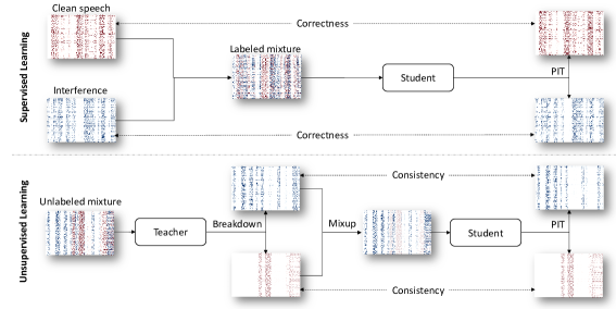
Fig. 1: Algorithmic flow of the Mixup-Breakdown training divided into the supervised and unsupervised learning procedures

Since large-scale, sufficiently varied training data with labels are often unattainable due to time and financial constraints, training a deep network of high complexity with a large number of parameters is prone to over-fitting and poor generalization. Therefore, we study a novel semi-supervised learning method called Mixup-Breakdown training (MBT) that exploits unlabeled data effectively to enhance generalization and reduce over-fitting.

As a typical training setup in speech separation, pairs of clean speech signal $\mathbf{s}$ and interference signal $\mathbf{e}$ add up into mixture signals $\mathbf{x}$ following randomly chosen signal-to-noise ratio (SNR) within specified range, resulting in a labeled training set of $N_{L}$ input-output pairs $\mathcal{D}_{L}=\{\mathbf{x}_{i},\mathbf{y}_{i}\}_{i=1}^{N_{L}}$, where $\mathbf{y}=(\mathbf{s},\mathbf{e})$, $\mathbf{x}=\mathbf{s}+\mathbf{e}$. Aside from the labeled data, in practice, unlabeled data $\mathcal{D}_{U}=\{\mathbf{x}_{j}\}_{j=N_{L}+1}^{N=N_{L}+N_{U}}$ are usually more authentic, attainable, yet under-explored.

In a supervised learning framework, given a speech separation model $\mathbf{f}_{\theta}$ with parameters $\theta$, an objective function $\mathcal{L}(\mathbf{f}_{\theta}(\mathbf{x}),\mathbf{y})$ is usually defined as the divergence between the predicted outputs $\mathbf{f}_{\theta}(\mathbf{x})=(\mathbf{\hat{s}},\mathbf{\hat{e}})$ and the original clean sources $\mathbf{y}$ to measure the “correctness of separation”, as shown in the upper algorithmic flow in Fig. 1. For example, we apply the recently proposed scale-invariant signal-to-noise ratio (SI-SNR) [8, 18] with PIT [6, 7]:

$$\mathcal{L}(\mathbf{f}_{\theta}(\mathbf{x}),\mathbf{y}) =\min_{\mathbf{u}\in\{\mathbf{\hat{s}},\,\mathbf{\hat{e}}\}}\mathcal{L}_{\text{SI-SNR}}(\mathbf{s},\mathbf{u})+\min_{\mathbf{v}\in\{\mathbf{\hat{s}},\,\mathbf{\hat{e}}\}}\mathcal{L}_{\text{SI-SNR}}(\mathbf{e},\mathbf{v}),$$ (1)

$$\mathcal{L}_{\text{SI-SNR}}(\mathbf{a},\mathbf{b}) =-10\log_{10}\frac{\lVert\Pi_{\mathbf{a}}(\mathbf{b})\rVert_{2}^{2}}{\lVert\mathbf{b}-\Pi_{\mathbf{a}}(\mathbf{b})\rVert_{2}^{2}},$$ (2)

where $\Pi_{\mathbf{a}}(\mathbf{b})=\mathbf{a}^{\top}\mathbf{b}/\lVert\mathbf{a}\rVert_{2}^{2}\cdot\mathbf{a}$ is a projection of $\mathbf{b}$ onto $\mathbf{a}$.

2.1 Conventional Supervised Learning

We first formalize the conventional supervised learning framework. Assuming that the input-output pairs follow a joint distribution $P(\mathbf{x},\mathbf{y})$, which is usually unknown, we minimize the average of the objective function over the joint distribution, i.e., the expected risk, to find an optimal set of parameters $\theta^{*}$:

$$\theta^{*} \approx\mathop{\arg\min}_{\theta}\int\mathcal{L}(\mathbf{f}_{\theta}(\mathbf{x}),\mathbf{y})\,d\,P_{\text{EMP}}(\mathbf{x},\mathbf{y};\mathcal{D}_{L})$$ (3)

$$=\mathop{\arg\min}_{\theta}\frac{1}{N_{L}}\sum_{i=1}^{N_{L}}\mathcal{L}(\mathbf{f}_{\theta}(\mathbf{x}_{i}),\mathbf{y}_{i}),$$ (4)

where in Eq.3, to approximate the unknown joint data distribution $P(\mathbf{x},\mathbf{y})$, an empirical distribution is used:

$$d\,P_{\text{EMP}}(\mathbf{x},\mathbf{y};\mathcal{D}_{L})=\frac{1}{N_{L}}\sum_{i=1}^{N_{L}}\delta(\mathbf{x}=\mathbf{x}_{i},\mathbf{y}=\mathbf{y}_{i})$$ (5)

where $\delta(\cdot)$ is a Dirac mass centered at $(\mathbf{x}_{i},\mathbf{y}_{i})$, so that the expected risk can estimate from the $N_{L}$ labeled training examples.

This conventional approach is also known as the empirical risk minimization (ERM) [19]. However, as highlighted in recent research [20, 9] as well as in classical learning theory [21], ERM has intrinsic limitations that the large neural networks trained with it memorize (instead of generalizing from) the training data; moreover, they are vulnerable to adversarial attacks, as they prone to produce drastically different predictions when giving examples just outside the training distribution. This evidence suggests that ERM is unable to generalize a model on testing distributions that differ only slightly from the training data. Our experiment in Section 4.3 also echoes this conclusion in mismatch training and test scenarios.

2.2 Mixup-Breakdown

The Mixup-Breakdown strategy is inspired from the fact that a human auditory system is capable of separating sources, not requiring any clean source for learning, yet having high consistency to perturbations such as high or low energies, fast or slow articulating speeds, moving or static locations, and with or without distortions.

As illustrated in the algorithmic flow of MBT in Fig. 1, we explore the interpolations between separated signals to provide a perturbation strategy to maintain the consistency of learning. We first introduce the Mixup and Breakdown operations:

$$\text{Mix}_{\lambda}(\mathbf{a},\mathbf{b})\triangleq\lambda\cdot\mathbf{a}+(1-\lambda)\cdot\mathbf{b}$$ (6)

$$\text{Break}_{\lambda}(\mathbf{a},\mathbf{b})\triangleq(\lambda\cdot\mathbf{a},\,\,(1-\lambda)\cdot\mathbf{b})$$ (7)

where $\mathbf{a}$ and $\mathbf{b}$ are two arbitrary signals, and $\lambda\sim\text{Beta}(\alpha,\alpha)$ for $\alpha\in(0,\infty)$ is inherited from the mixup approach [9].

The Mixup-Breakdown (MB) strategy trains a student model $\mathbf{f}_{\theta_{S}}$ to provide consistent predictions with the teacher model $\mathbf{f}_{\theta_{T}}$ of the same network structure at perturbations of predicted separations from the input mixtures (either labeled or unlabeled):

$$\mathbf{f}_{\theta_{S}}(\text{Mix}_{\lambda}(\mathbf{f}_{\theta_{T}}(\mathbf{x}_{j})))\approx\text{Break}_{\lambda}(\mathbf{f}_{\theta_{T}}(\mathbf{x}_{j}))$$ (8)

where the teacher model parameters $\theta_{T}$ is an exponential moving average of the student model parameters $\theta_{S}$. It has been proven that averaging model parameters over training steps tends to generate a more accurate model than directly using the final parameters [22, 14], resulting in better generalization performance.

Meanwhile, adding perturbation to the estimated separations is likely to construct more useful pseudo labeled input-output pairs nearer to the separation boundary, on which the consistency regularization should apply. Mathematically, the MB operation can view as a generic augmentation of the empirical distribution:

$$d\,P_{\text{MBT}}(\mathbf{\tilde{x}},\mathbf{\tilde{y}};\mathcal{D})=\frac{1}{N}\sum_{i=1}^{N}\bm{v}(\mathbf{\tilde{x}},\mathbf{\tilde{y}}|\mathbf{x}_{i})$$ (9)

$$\bm{v}(\mathbf{\tilde{x}},\mathbf{\tilde{y}}|\mathbf{x}_{i})=\mathbb{E}_{\lambda}\left[\delta\left(\mathbf{\tilde{x}}=\text{Mix}_{\lambda}(\mathbf{f}_{\theta_{T}}(\mathbf{x}_{i})),\mathbf{\tilde{y}}=\text{Break}_{\lambda}(\mathbf{f}_{\theta_{T}}(\mathbf{x}_{i}))\right)\right]$$ (10)

In a semi-supervised learning setting, provided the dataset $\mathcal{D}$ composed of the labeled dataset $\mathcal{D}_{L}$ and the unlabeled dataset $\mathcal{D}_{U}$, we present a new consistency-based training method, namely, Mixup-Breakdown Training (MBT):

$$\theta^{*}_{S}\approx\mathop{\arg\min}_{\theta_{S}} \underbrace{\left[\int\mathcal{L}(\mathbf{f}_{\theta_{S}}(\mathbf{x}),\mathbf{y})\,d\,P_{\text{EMP}}(\mathbf{x},\mathbf{y};\mathcal{D}_{L})\right.}_{\text{Correctness}}+$$ (11)

$$r(t)\underbrace{\left.\int\mathcal{L}(\mathbf{f}_{\theta_{S}}(\mathbf{\tilde{x}}),\mathbf{\tilde{y}})\,d\,P_{\text{MBT}}(\mathbf{\tilde{x}},\mathbf{\tilde{y}};\mathcal{D})\right]}_{\text{Consistency}}$$ (12)

$$=\mathop{\arg\min}_{\theta_{S}} \left[\frac{1}{N_{L}}\sum_{i=1}^{N_{L}}\mathcal{L}(\mathbf{f}_{\theta_{S}}(\mathbf{x}_{i}),\mathbf{y}_{i})+\right.$$ (13)

$$\left.\frac{r(t)}{N}\sum_{j=1}^{N}\mathcal{L}(\mathbf{f}_{\theta_{S}}(\text{Mix}_{\lambda}(\mathbf{f}_{\theta_{T}}(\mathbf{x}_{j}))),\,\,\text{Break}_{\lambda}(\mathbf{f}_{\theta_{T}}(\mathbf{x}_{j})))\right],$$ (14)

where $r(t)$ is the ramp function that increases the importance of the consistency term as the training goes [14].

2.2.1 Data Augmentation Effect Using Unlabeled Data

Data augmentation is a widely adopted technique to improve the generalization of a supervised model. For example, in image classification, new images are produced by shifting, zooming in/out, rotating, or flipping images [23]; likewise, in speech recognition, the training data are augmented using varied vocal tract length [24], SNR, tempo, and speed perturbation [25], etc. However, these approaches mostly confine to labeled data. Notably, some recent research, including the mixup technology [9] and generative adversarial networks (GANs), has also contributed to generic data augmentation methods [26, 27, 17].

Unlike GANs that require training an additional model and increasing the complexity, our MBT can be easily implemented with minimal computational overhead. By observing Eq. 14, we can use MBT to manipulate both labeled data (i.e., for $j\in\{1,...,N_{L}\}$) and unlabeled data (i.e., for $j\in\{N_{L}+1,...,N\}$) to produce pseudo “labeled” input-output pairs outside the empirical distribution. Although, in this paper we focus on amplitude interpolation (Eq. 6 and 7) like different SNR augmentation, the MBT methodology is straightforward to extend to other types of perturbations, such as various distortions, speeds, and locations (for multi-channel scenarios). Therefore we consider that the proposed MBT is promising and may enlighten a new generic way to exploit unlabeled data.

3 Related Work

Among all consistency-based methods, the recent interpolation consistency training (ICT) [17] have achieved the state-of-the-art results in computer vision (CV) benchmarks. The main difference of the ICT from the MT [14] is the use of the aforementioned mixup technique when calculating the consistency loss:

$$\mathcal{L}_{\text{ICT}}=\mathcal{L}(\mathbf{y}_{i},\mathbf{f}_{\theta_{S}}(\mathbf{x}_{i}))+r(t)\mathcal{C}(\mathbf{x}_{j},\mathbf{x}_{k})$$ (15)

$$\mathcal{C}(\mathbf{x}_{j},\mathbf{x}_{k})=\left\|\mathbf{f}_{\theta_{S}}\left(\text{Mix}_{\lambda}(\mathbf{x}_{j},\mathbf{x}_{k})\right)-\text{Mix}_{\lambda}(\mathbf{f}_{\theta_{T}}(\mathbf{x}_{j}),\mathbf{f}_{\theta_{T}}(\mathbf{x}_{k}))\ \right\|^{2}_{2}$$ (16)

for $(\mathbf{x}_{i},\mathbf{y}_{i})\sim\mathcal{D}_{L},\mathbf{x}_{j},\mathbf{x}_{k}\sim\mathcal{D}_{U}$. Note that the mixup here is on two input samples randomly drawn from the unlabeled data, which is fundamentally different from MBT.

As reported by the authors, ICT outperforms other cutting-edge SSL methods, including MT, with high significance in benchmark CV datasets. Therefore, we will analyze its performance as another strong baseline. Meanwhile, we use ICT as an ablation study to validate the necessity of the “Breakdown” part in our “Mixup-Breakdown” methodology.

4 Experiments

4.1 Experimental Setup

4.1.1 Data Preparation

To test our hypothesis that conventional models could abruptly fail when separating mixture signals that contain mismatch interference between test and training, we built three new datasets of speech mixtures based on the WSJ0-2mix corpus [28] by replacing the background speech (the one with the lower SNR) with other types of interference :

• WSJ0-Libri: using clean speech drawn from the publicly available Librispeech 100h training corpus [29].

• WSJ0-music: using music clips drawn from a 43-hour music dataset that contains various classical and popular music genres, e.g., baroque, classical, romantic, jazz, country, and hip-hop.

• WSJ0-noise: using noise clips drawn from a 4-hour recording collected in various daily life scenarios such as office, restaurant, supermarket, and construction place.

Note that each of the above new datasets follows the same SNR range as WSJ0-2mix, and contains non-overlapping train, dev, and test set like WSJ0-2mix. We also combined all the above unlabeled datasets into one union unlabeled dataset denoted as WSJ0-multi.

4.1.2 Implementation Details

We implemented the mixup, MT, ICT, and our proposed MBT to train the state-of-the-art speech separation model – Conv-TasNet [8] for comparative performance analysis. The Conv-Tasnet model architecture was replicated exactly from [8]. In all SSL settings including MT, ICT and our MBT method, we set the same decay coefficient for the mean-teacher to 0.999 to remain conservativeness following [14], and the same ramp function $r(t)=\exp(t/T_{\text{max}}-1)$ for $t\in\{1,...,T_{\text{max}}\}$, where $T_{\text{max}}=100$ was the maximum number of epochs. Besides, we set $\alpha=1$ following [9], so that $\lambda$ becames uniformly distributed in $[0,1]$.

4.2 MBT for Supervised Learning

Table 1: Comparison of performances on the WSJ0-2mix dataset. $\star$: Results in our implementation.

Method	Params.	Trained	SI-SNRi
DPCL++[1]	13.6M		10.8
DANet [2]	9.1M		10.5
ADANet [4]	9.1M	WSJ0-2mix	10.4
Chimera++ [30]	32.9M		11.5
WA-MISI-5 [31]	32.9M		12.6
BLSTM-TasNet [32]	23.6M		13.2
⋆Conv-TasNet	8.8M		15.3
		WSJ0-2mix+
⋆MBT	8.8M	“online” data	15.5
		augmentation
		WSJ0-2mix+
⋆MBT	8.8M	Unlabeled	15.6
		WSJ0-multi

First, we conducted a benchmark evaluation on the WSJ0-2mix dataset without using any unlabeled data to examine the performance of MBT simply as an “online” data augmentation for purely supervised learning. This learning was done by directly computing the consistency loss only on the labeled data, i.e., let $\mathcal{D}=\{\mathbf{x}_{i}\}_{i=1}^{N_{L}}$. The separation performances of different supervised systems on the WSJ0-2mix dataset shows in Table 1. Despite the very strong Conv-TasNet as baseline, by replacing the conventional ERM with MBT in Conv-TasNet, MBT managed to enhance the performance by $0.2$ and $0.3$ absolute SI-SNRi and SDRi improvement respectively.

4.3 Generalization Capability

Since MBT suited both supervised learning and SSL framework, for training Conv-TasNet, we compared MBT with two sets of reference approaches: 1) supervised learning methods including the ERM and the mixup, and 2) SSL methods including the MT and the ICT.

The goal in this section was to study and compare the generalization capability of different methods. For training the SSL models, we assume they have access to the corresponding unlabeled training sets of WSJ0-Libri, WSJ0-noise, and WSJ0-music. Each model was then evaluated on the test sets of WSJ0-Libri, WSJ0-noise, and WSJ0-music, representing different kinds of interference with increasing degrees of mismatch.

4.3.1 Mismatch Speech Interference

The first task evaluated two-talker speech separation with mismatch speech interference between training and inference. In the supervised learning setting, as shown in the upper half of Table 2, MBT obtained higher SI-SNRi over the ERM and the mixup baseline; in the SSL setting, it also outperformed the MT and the ICT.

Table 2: Separation performance of different training approaches in the presence of mismatch speech interference

Method	Trained on	Tested on	SI-SNRi
ERM			13.56
mixup	WSJ0-2mix		13.58
MBT			13.75
MT	WSJ0-2mix+	WSJ0-Libri	13.81
ICT	Unlabeled WSJ0-Libri		13.78
MBT			13.95
MBT	WSJ0-2mix+		13.88
	Unlabeled WSJ0-multi

4.3.2 Mismatch Background Noise Interference

Moreover, we tested the robustness of the separation models in the case of unseen background noise collected in real-world environments. We supposed this task might be less challenging than separating the two-talker speech mixture since background noise tends to be stationary, yet, unexpectedly, as shown in the upper half of Table 3, all supervised learning systems failed to retain the performance of what has achieved in domain of WSJ0-2mix. The result reflects the semi-supervised learning is crucial for a robust separation system, as shown in the lower half of Table 3, that it can achieve high and much more acceptable separation performance than the supervised systems in a new domain without any labeled data. Consistently, the MBT outperformed the MT and ICT by $0.7$ and $0.85$ absolute SI-SNRi improvement, respectively.

Table 3: Separation performance of different training approaches in the presence of mismatch background noise interference

Method	Trained on	Tested on	SI-SNRi
ERM	WSJ0-2mix		1.86
mixup			1.91
MBT			2.10
MT	WSJ0-2mix +	WSJ0-noise	12.51
ICT	Unlabeled WSJ0-noise		12.36
MBT			13.21
MBT	WSJ0-2mix +		13.52
	Unlabeled WSJ0-multi

4.3.3 Mismatch Music Interference

The third task was considered the most challenging since the music interference was highly non-stationary and was of a completely out-domain audio type. Similar to the result in Sec 4.3.2, the upper half in Table 4 indicates all supervised systems were drastically degraded to around $2$ SI-SNRi, whereas the systems trained with semi-supervised learning could remain high standard of performance, in which MBT produced significantly higher SI-SNRi than both MT and ICT with up to $13.77\%$ relative improvement.

Table 4: Separation performance of different training approaches in the presence of mismatch music interference

Method	Trained on	Tested on	SI-SNRi
ERM	WSJ0-2mix		1.93
mixup			1.94
MBT			1.99
MT	WSJ0-2mix +	WSJ0-music	14.12
ICT	Unlabeled WSJ0-music		14.02
MBT			15.95
MBT	WSJ0-2mix +		15.67
	Unlabeled WSJ0-multi

5 Conclusions

This paper introduces a novel training method called Mixup-Breakdown training (MBT). It can significantly improve the generalization of the state-of-the-art speech separation models over the standard training framework. The contribution of MBT is mainly two-fold: First, when given only labeled data, MBT can serve as a superior data augmentation technique for speech separation; secondly, when provided with a large amount of unlabeled speech mixture signals that possibly contain mismatch interference, MBT can effectively exploit the unlabeled data to enhance the generalization power of separation model with a minimal computational overhead. Our results indicate that MBT can remain strong performance even in non-specific domain. We will explore more perturbation types for MBT to further unleash its generalization capability in future work.

References

- [1] Yusuf Isik, Jonathan Le Roux, Zhuo Chen, Shinji Watanabe, and John R Hershey, “Single-channel multi-speaker separation using deep clustering,” Proc. INTERSPEECH, 2016.
- [2] Zhuo Chen, Yi Luo, and Nima Mesgarani, “Deep attractor network for single-microphone speaker separation,” in Proc. ICASSP. IEEE, 2017, pp. 246–250.
- [3] Jun Wang, Jie Chen, Dan Su, Lianwu Chen, Meng Yu, Yanmin Qian, and Dong Yu, “Deep extractor network for target speaker recovery from single channel speech mixtures,” arXiv preprint arXiv:1807.08974, 2018.
- [4] Yi Luo, Zhuo Chen, and Nima Mesgarani, “Speaker-independent speech separation with deep attractor network,” TASLP, vol. 26, no. 4, pp. 787–796, 2018.
- [5] Chenglin Xu, Wei Rao, Xiong Xiao, Eng Siong Chng, and Haizhou Li, “Single channel speech separation with constrained utterance level permutation invariant training using grid lstm,” in Proc. ICASSP. IEEE, 2018, pp. 6–10.
- [6] Dong Yu, Morten Kolbæk, Zheng-Hua Tan, and Jesper Jensen, “Permutation invariant training of deep models for speaker-independent multi-talker speech separation,” in Proc. ICASSP. IEEE, 2017, pp. 241–245.
- [7] Morten Kolbæk, Dong Yu, Zheng-Hua Tan, Jesper Jensen, Morten Kolbaek, Dong Yu, Zheng-Hua Tan, and Jesper Jensen, “Multitalker speech separation with utterance-level permutation invariant training of deep recurrent neural networks,” TASLP, vol. 25, no. 10, pp. 1901–1913, 2017.
- [8] Yi Luo and Nima Mesgarani, “Conv-tasnet: Surpassing ideal time-frequency masking for speech separation,” IEEE/ACM Transactions on Audio, Speech, and Language Processing (TASLP), vol. 27, pp. 1256–1266, 2019.
- [9] Hongyi Zhang, Moustapha Cisse, Yann N Dauphin, and David Lopez-Paz, “mixup: Beyond empirical risk minimization,” 6th International Conference on Learning Representations (ICLR), 2018.
- [10] Olivier Chapelle, Bernhard Scholkopf, and Alexander Zien, “Semi-supervised learning (chapelle, o. et al., eds.; 2006)[book reviews],” IEEE Transactions on Neural Networks, vol. 20, no. 3, pp. 542–542, 2009.
- [11] Antti Rasmus, Mathias Berglund, Mikko Honkala, Harri Valpola, and Tapani Raiko, “Semi-supervised learning with ladder networks,” in Advances in neural information processing systems (NIPS), 2015, pp. 3546–3554.
- [12] Mehdi Sajjadi, Mehran Javanmardi, and Tolga Tasdizen, “Regularization with stochastic transformations and perturbations for deep semi-supervised learning,” in NIPS, 2016, pp. 1163–1171.
- [13] Samuli Laine and Timo Aila, “Temporal ensembling for semi-supervised learning,” arXiv preprint arXiv:1610.02242, 2016.
- [14] Antti Tarvainen and Harri Valpola, “Mean teachers are better role models: Weight-averaged consistency targets improve semi-supervised deep learning results,” in NIPS, 2017, pp. 1195–1204.
- [15] Takeru Miyato, Shin-ichi Maeda, Masanori Koyama, and Shin Ishii, “Virtual adversarial training: a regularization method for supervised and semi-supervised learning,” IEEE transactions on pattern analysis and machine intelligence, vol. 41, no. 8, pp. 1979–1993, 2018.
- [16] Yucen Luo, Jun Zhu, Mengxi Li, Yong Ren, and Bo Zhang, “Smooth neighbors on teacher graphs for semi-supervised learning,” in Proc. CVPR, 2018, pp. 8896–8905.
- [17] Vikas Verma, Alex Lamb, Juho Kannala, Yoshua Bengio, and David Lopez-Paz, “Interpolation consistency training for semi-supervised learning,” arXiv preprint arXiv:1903.03825, 2019.
- [18] Gene-Ping Yang, Chao-I Tuan, Hung-Yi Lee, and Lin-shan Lee, “Improved speech separation with time-and-frequency cross-domain joint embedding and clustering,” arXiv preprint arXiv:1904.07845, 2019.
- [19] Vladimir Vapnik, “Statistical learning theory,” 1998.
- [20] Chiyuan Zhang, Samy Bengio, Moritz Hardt, Benjamin Recht, and Oriol Vinyals, “Understanding deep learning requires rethinking generalization,” ICLR, 2017.
- [21] V. Vapnik and A. Y. Chervonenkis, “On the uniform convergence of relative frequencies of events to their probabilities,” Theory of Probability and its Applications, 1971.
- [22] B. T. Polyak and A. B. Juditsky, “Acceleration of stochastic approximation by averaging,” SIAM J. Control Optim., vol. 30(4), 1992.
- [23] Esben Jannik Bjerrum, “Smiles enumeration as data augmentation for neural network modeling of molecules,” arXiv preprint arXiv:1703.07076, 2017.
- [24] Navdeep Jaitly and Geoffrey E Hinton, “Vocal tract length perturbation (vtlp) improves speech recognition,” in Proc. ICML Workshop on Deep Learning for Audio, Speech and Language, 2013, vol. 117.
- [25] Tom Ko, Vijayaditya Peddinti, Daniel Povey, and Sanjeev Khudanpur, “Audio augmentation for speech recognition,” in Sixteenth Annual Conference of the International Speech Communication Association, 2015.
- [26] Ian Goodfellow, Jean Pouget-Abadie, Mehdi Mirza, Bing Xu, David Warde-Farley, Sherjil Ozair, Aaron Courville, and Yoshua Bengio, “Generative adversarial nets,” in NIPS, 2014, pp. 2672–2680.
- [27] Antreas Antoniou, Amos Storkey, and Harrison Edwards, “Data augmentation generative adversarial networks,” arXiv preprint arXiv:1711.04340, 2017.
- [28] John R Hershey, Zhuo Chen, Jonathan Le Roux, and Shinji Watanabe, “Deep clustering: Discriminative embeddings for segmentation and separation,” in Proc. ICASSP. IEEE, 2016, pp. 31–35.
- [29] Vassil Panayotov, Guoguo Chen, Daniel Povey, and Sanjeev Khudanpur, “Librispeech: an asr corpus based on public domain audio books,” in Proc. ICASSP. IEEE, 2015, pp. 5206–5210.
- [30] Zhong-Qiu Wang, Jonathan Le Roux, and John R Hershey, “Alternative objective functions for deep clustering,” in Proc. ICASSP. IEEE, 2018, pp. 686–690.
- [31] Zhong-Qiu Wang, Jonathan Le Roux, DeLiang Wang, and John R Hershey, “End-to-end speech separation with unfolded iterative phase reconstruction,” arXiv preprint arXiv:1804.10204, 2018.
- [32] Yi Luo and Nima Mesgarani, “Real-time single-channel dereverberation and separation with time-domain audio separation network.,” in Proc. INTERSPEECH, 2018, pp. 342–346.