Phase separation in a two-dimensional binary colloidal mixture by quorum sensing activity

Abstract

We present results from Langevin dynamics simulations of a glassy active-passive mixture of soft-repulsive binary colloidal disks. Activity on the smaller particles is applied according to the quorum sensing scheme, in which a smaller particle will be active for a persistence time if its local nearest neighbors are equal to or greater than a certain threshold value. We start with a passive glassy state of the system and apply activity to the smaller particles, which shows a non-monotonous glassy character of the active particles with the persistence time of the active force, from its passive limit (zero activity). On the other hand, passive particles of the active-passive mixture phase separate at the intermediate persistence time of the active force, resulting in the hexatic-liquid and solid-liquid phases. Thus, our system shows three regimes as active glass, phase separation, and active liquid, as the persistence time increases from its smaller values. We show that the solidlike and hexatic phases consisting of passive large particles are stable due to the smaller momentum transfer from active to passive particles, compared to the higher persistence time where the positional and orientational ordering vanishes. Our model is relevant to active biological systems, where glassy dynamics is present, e.g., bacterial cytoplasm, biological tissues, dense quorum sensing bacteria, and synthetic smart amorphous glasses.

I Introduction

Active (self-propelled) particles consume energy from within the system or by some external means, and drive themselves to a non-equilibrium state Ramaswamy (2010); Bechinger et al. (2016). Systems with self-propelled particles are of great interest from the perspective of fundamental physics and they are ubiquitous. Examples of living active matter systems are, but not limited to, sperm swarming Guidobaldi et al. (2014), bird-flocking and fish schools Krause and Ruxton (2002), biological microswimmers Berg and Turner (1979), quorum sensing bacteria Papenfort and Bassler (2016) etc. Another class of active systems is synthetic active matter; examples include artificial microswimmers Bechinger et al. (2016), active mechanical (micro and nano) robots Li et al. (2017), and synthetic quorum sensing systems B$\ddot{a}$uerle et al. (2018) that are useful for the targeted drug delivery, directed mechanical work, biomarkers, and local-density-dependent motility. Motile bacteria sense a local concentration of the signaling molecules and themselves (e.g., acyl-homoserine lactones in Gram-negative bacteria) to perform virulence, biofilm formation, etc., which is termed as quorum sensing (QS) Whiteley et al. (2017). Bacteria use QS to produce, release, and sense the extracellular chemical signals that are called as autoinducer molecules for cell-cell communication. The number of autoinducer molecules increases as a function of the bacterial cell density, which activate its gene transcriptions at a cell density threshold: bacteria perform QS at both low and high cell density thresholds Jung et al. (2015).

Several living systems including bacterial cytoplasm and collective cell migration, show the fingerprints of glassy dynamics Parry et al. (2014); Janssen (2019). Glasses are dense amorphous systems, and one of the hallmarks of the glassy systems is a dramatic slowdown of the density relaxations with a minimal change in their structure Berthier and Biroli (2011). The glassy dynamics of the bacterial cytoplasm arises from its crowded (dense) intracellular components, which fluidizes by the metabolic activities of the bacterial cell, showing an active glassy characteristic Parry et al. (2014). Another class of active-glass systems are smart amorphous materials (artificial systems) including phase-changing materials and self-healing glasses Janssen (2019). Experimental study of these active materials is difficult at high density, where the corresponding passive system shows glassiness. Very recently, Klongvessa et al. performed an experiment on the gold colloidal particles that are called as active Janus colloids, half coated with platinum at high volume fractions Klongvessa et al. (2019). The authors concluded that active glass slows down at the smaller activity, whereas its fluidization enhances at the higher activity, which is a non-monotonous character of the active glassy Janus colloids. Simulation studies by Szamel and Berthier Berthier et al. (2017, 2019) also show the non-monotonous character in the (all-)active glassy binary colloidal mixture. Another simulation study of the active-passive binary mixture shows that activity fluidizes the glassy state Mandal et al. (2016).

Active DNAs in the interphase of chromosome drive to the segregated domains, consisting of euchromatin and heterochromatin that is explained from the phase separation of active-passive components Strom et al. (2017). Recently, a study of activity-induced phase separation in the monodisperse soft-repulsive active-passive disks by Stenhammer et al. Stenhammar et al. (2015) showed the presence of segregated active and passive domains, where the compression waves originating from the corona of active particles causes the crystallization of the passive particles. In a soft-repulsive active dumbbells system, the liquid (or gas) and hexatic phase coexist, as reported by Cugliandolo et al. Cugliandolo et al. (2017). These studies also showed that the motility-induced phase separation (see Ref. Geyer et al. (2019) and references therein), where phase separation occurs at a threshold value of the activity, which is not true in general. Thus, it prompts us to study the activity-induced phase separation in a dense active-passive mixture. In this study, we simulate a two-dimensional (2D) binary colloidal mixture consisting of small and large size particles in its glassy state. The small particles are kept motile depending upon their local nearest neighbors (local density), $n_{b}^{fcs}$, to replicate the local density-dependent sensing in QS bacteria. Thus, our system could be a model system for the smart amorphous materials, and the QS in crowded bacteria. We use three control parameters in our simulations: activity $f_{a}$, persistence time $\tau_{p}$, and the $n_{b}^{fcs}$ that determines the number density of the active particles in our system. Starting from the passive glass, the active system shows enhanced glassiness at smaller $\tau_{p}$ (mixed-phase), which first phase separate into hexatic-liquid and then to the solid-liquid at the intermediate $\tau_{p}$; solidlike and hexatic phases in the phase separation regime are consist of only the large (passive) particles. On further increment in $\tau_{p}$, activity $f_{a}$ fluidizes both species of the particles that undergo mixing. Thus, our system shows a continuous increase in hexatic order from its passive limit, which becomes solidlike at the intermediate $\tau_{p}$. This solidlike phase melts into the hexatic phase, which subsequently becomes liquid at the higher $\tau_{p}$.

II Model and simulation details

In this section, we discuss Langevin dynamics simulations, the QS activity, and an initial configuration of our 2D binary colloidal system.

II.1 Equations of motion

We simulate a 50:50 mixture, consisting of 1000 soft colloidal disks of size ratio 1:1.4 that has sufficient frustration to prevent crystallization, and is a well-known glass-forming system Hamanaka and Onuki (2006); Kawasaki and Tanaka (2011). Equations of motion for the colloidal disks are of stochastic type, i.e., Langevin equations

$$m_{i}\ddot{\mathbf{r}_{i}}=-\gamma\dot{\mathbf{r}_{i}}+\sum_{ij}\mathbf{F}_{ij}+\mathbf{F}^{a}_{i}+{\sqrt{2k_{B}T\gamma}}{\boldsymbol{\eta}_{i}},$$ (1)

where $\gamma$ is the friction coefficient, $\mathbf{F}_{ij}=-\boldsymbol{\nabla}V(r_{ij})$ is the inter-particle interaction force, $T$ is the thermal noise temperature, $\mathbf{F}^{a}_{i}$ is an active force of magnitude $f_{a}$, and $\eta_{i}$ is the random gaussian noise with zero mean and unit variance, i.e., $\langle\eta_{i}\rangle=$0 and $\langle\eta_{i\alpha}(t)\eta_{j\beta}(t^{\prime})\rangle=\delta_{ij}\delta_{\alpha\beta}\delta(t-t^{\prime})$. Inter-particle interactions are modelled by purely repulsive and soft Lennard-Jones potential Hansen and McDonald (2006)

$$V(r_{ij})=4\epsilon\left[\left(\frac{\sigma_{\alpha\beta}}{r_{ij}}\right)^{12}-\left(\frac{\sigma_{\alpha\beta}}{r_{ij}}\right)^{6}+\frac{1}{4}\right],$$ (2)

with cut-off at $r^{\alpha\beta}_{c}=2^{1/6}\sigma_{\alpha\beta}$. Here $(\alpha,\beta)\in(A,B)$, $\epsilon=$ 1.0, $\sigma_{AA}=$ 1.4 $\sigma_{BB}$, $\sigma_{AB}=$ 1.2 $\sigma_{BB}$, and $\sigma_{BB}=$ 1.0; distances are measured in the units of $\sigma_{BB}$. For the underdamped case, we use $\gamma=$ 10.0. The system is simulated at a constant area fraction $\phi=$ 0.628 that is calculated as $\phi=\pi\rho(\sigma^{2}_{AA}+\sigma^{2}_{BB})/8$. The equations of motion are integrated using a second-order scheme given by Vanden-Eijnden and Ciccotti Vanden-Eijnden and Ciccotti (2006), using the time step $dt=$ 0.002, for active and corresponding passive system. Note that the active system will become passive in the limit of activity $f_{a}=$ 0 (zero active force). All the quantities presented here are in the Lennard-Jones (reduced) units, i.e., reduced density $\rho^{*}=\rho\sigma^{3}$, reduced temperature $T^{*}=k_{B}T/\epsilon$, reduced time $t^{*}=(\epsilon/{m\sigma^{2}})^{1/2}t$, and reduced force $f^{*}=f\sigma/\epsilon$ Hansen and McDonald (2006).

II.2 Quorum sensing activity

QS bacteria uses local (neighboring) density detection algorithm to express their genes, virulence, biofilm formation etc. Papenfort and Bassler (2016); Whiteley et al. (2017); B$\ddot{a}$uerle et al. (2018). To replicate the behavior of QS bacteria, we simulate the binary colloidal mixture in two dimensions in which only small particles are active according to the local density searching algorithm for a finite persistence time of the active force. Note that all $A$ (large) particles are passive throughout the simulations. For the range of local density sensing algorithm, we compute radial distribution function (RDF) of $B$ particles for the passive system at $T=$ 0.01 and $\phi=$ 0.628 as

$$g_{B}(r)=\frac{A}{2\pi r\Delta rNN_{B}}\left\langle\sum_{i=1}^{N_{B}}\sum_{\begin{subarray}{c}j=1\\ j\neq i\end{subarray}}^{N}\delta({r-|\mathbf{r}_{j}-\mathbf{r}_{i}|})\right\rangle,$$ (3)

which is shown in Fig. 1(d). Here, $A$ is the area of the two-dimensional simulation box, $N$ and $N_{B}$ are total number of particles and number of $B$ particles in the system, respectively. The $g_{B}(r)$ computes number of $B$ and $A$ particles around a tagged $B$ particle, its first peak corresponds to the $B-B$ particles, whereas the second peak corresponds to the $B-A$ particles. A minima at $r=$ 1.825, after the second peak, shown by red dot-dashed line in Fig. 1(d), corresponds to the first coordination shell (FCS) of $g_{B}(r)$. We compute number of nearest-neighbors (both $A$ and $B$) of each $B$ particle within the FCS. A small ($B$) particle is active according to a criterion that if its $N_{nn}^{i}>=n^{fcs}_{b}$. Here, $N_{nn}^{i}$ is the instantaneous number of nearest neighbors of a $B$ particle within the FCS [see Figs. 1(b) and 1(d)] and the $n^{fcs}_{b}$ is a fixed threshold value for the number of nearest neighbors of $B$ particles. We scan $N_{nn}^{i}$ of each $B$ particle at each $t=\tau_{p}$, where $\tau_{p}$ is the persistence time of the active force. In this study, we present results from the $n^{fcs}_{b}=$ 4 and 5. At $n^{fcs}_{b}=$ 6, only $10-15\%$ of the $B$ particles are active (data not presented in this study, which will be reported elsewhere), and at $n^{fcs}_{b}=$ 7 only $1-5$ $B$ particles are active. Thus, the number density of active $B$ particles, $\rho_{ab}$, is controlled by the QS scheme; the range of $\rho_{ab}=0.256-0.27$ for $n_{b}^{fcs}=$ 4 and $\rho_{ab}=0.2-0.265$ for $n_{b}^{fcs}=$ 5. The shift in the range of $\rho_{ab}$ towards its smaller values is natural for $n_{b}^{fcs}=$ 5, as the number of $B$ particles with $N_{nn}^{i}=$ 5 or greater decrease compared to the $n_{b}^{fcs}=$ 4, at the same volume fraction. Thus, the number density of active particles in our study is varying and according to the QS rules using the local neighbor searching algorithm.

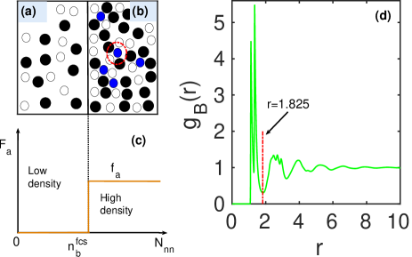
Figure 1: (a–c) Schematic diagram for the quorum sensing: (a) Passive binary mixture, (b) active-passive binary mixture, (c) quorum sensing rule at high density. In (a) and (b), open small circles are passive $B$ (small) particles, whereas filled black circles are passive $A$ (large) particles. In (b) filled blue circles are the active $B$ (small) particles and red dot-dashed circle represents the FCS of one of the active particles. (d) RDF of $B$ particles. The red dot-dashed line at $r=$ 1.825 corresponds to the FCS in $g_{B}(r)$.

We apply active force on $B$ particles according the QS scheme described above for the finite persistence time $\tau_{p}$ in the range $0.01-20.0$. The active force $\mathbf{F}_{a}^{i}$ [see Eq. 1] on an $i$th particle is given as $\mathbf{F}_{a}^{i}=f_{a}\boldsymbol{\zeta}_{i}$, where $f_{a}$ is a magnitude of the active force. Figure 1(c) shows that if a $B$ particle satisfies the criterion mentioned above then it is active with the activity $f_{a}$, otherwise it is passive and $f_{a}=$ 0. The direction of the active force on an $i^{th}$ particle is given by $\boldsymbol{\zeta}_{i}=\zeta_{ix}\hat{\boldsymbol{x}}+\zeta_{iy}\hat{\boldsymbol{y}}$ as

$$\langle\zeta_{i\alpha}(t)\zeta_{j\beta}(t^{\prime})\rangle=\delta_{ij}\delta_{\alpha\beta},$$ (4)

for $|t-t^{\prime}|<=\tau_{p}$ and zero otherwise; $(\alpha,\beta)\in(x,y)$. The $\zeta_{ix}$ and $\zeta_{iy}$ are between $-1$ and $+1$, chosen from the uniform random deviates.

II.3 Initial configurations

We prepare a random initial configuration of the passive binary colloidal mixture at the area fraction $\phi=$ 0.628, which is shown in Fig. 2(a). This random initial configuration is equilibrated at temperature $T=$ 8.0 using the Langevin dynamics simulations. Final configuration of the equilibrated system is quenched from $T=$ 8.0 to $T=$ 0.01, which is equilibrated for $5\times 10^{7}$ steps, and then trajectories are stored up to $2.5\times 10^{6}$ steps. The equilibrated configuration of the passive system at $T=$ 0.01, is used as an initial configuration for the active system. Thus, the active-passive binary mixture at all activities and persistence times runs for the $5\times 10^{7}$ steps to reach its steady state, after that, trajectories of the system are stored for analysis purpose. To examine local orientational ordering in the passive system, we invoke single particle hexatic order parameter (HOP) that entails information about the local hexatic order in two dimensions. The HOP is defined as

$$\psi_{6}^{j}=\frac{1}{N_{b}^{j}}\sum_{m=1}^{N_{b}^{j}}\exp(\imath 6\theta_{j}^{m}),$$ (5)

where $N_{b}^{j}$ are the number of nearest neighbors of a particle $j$, $\theta_{j}^{m}$ is the angle between the radius vector $\mathbf{r}_{j}^{m}$ and the reference axis Binder et al. (2002); Hamanaka and Onuki (2006). Depending upon the $\theta_{j}^{m}$, values of the $|\psi_{6}^{j}|$ ranges from 0 to 1; a perfect trigonal corresponds to the $6\theta_{j}^{m}=2\pi$ that has a value $|\psi_{6}^{j}|=$ 1, whereas $|\psi_{6}^{j}|=$ 0 corresponds to a random orientational arrangement of six nearest-neighbors of a particle $j$. We use cut-off distances $2.085$ and $1.825$, respectively as the second minima of $g_{A}(r)$ and $g_{B}(r)$, for calculating nearest-neighbors of $A$ and $B$ particles; for reference the $g_{B}(r)$ is shown in the Fig. 1(d). The absolute values of $\psi_{6}^{j}$ of majority of particles for the random initial configuration (see Fig. 2(a)), are far less than 1.0, showing a random orientational order, except for few particles, for them it shows local hexatic ordering ($|\psi_{6}^{j}|\approx$ 1) because the natural number of nearest neighbors of a particle are six in a dense 2D system. The equilibrated final configuration of the passive system at $T=$ 0.01 shows the local hexatic ordering of $A$ and $B$ particles that can be seen in Fig. 2(b). Fig. 2(b) shows that the local hexatic ordering increases in the passive system at $T=$ 0.01 and the system shows mixing. Structural analysis of the passive system is given in Appendix A, which shows that it is amorphous and does not posses long-range (or quasi-long-range) positional or orientational order.

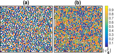
Figure 2: (a) Random initial configuration of the Passive mixture at $\phi=$ 0.628, (b) Final configuration of the Passive mixture at $T=$ 0.01 and $\phi=$ 0.628. Black (large) and red (small) edge spheres correspond to the $A$ and $B$ particles. Face color of the particles is according to the color bar for local hexatic order parameter, $|\psi_{6}^{j}|$.

III Results and discussion

III.1 Configurations of active-passive binary mixture

The final configuration obtained at $T=$ 0.01, shown in Fig. 2(b), is used as an initial configuration for the active system ($f_{a}\neq$ 0). As discussed in Sec. II.2 that we apply activity to only smaller particles according to the QS rules. We vary the activity and the persistence time of the active force as $f_{a}=$1-10 and $\tau_{p}=$ 0.01-20.0, respectively, for this study. In Fig. 3, we show few typical configurations of the active-passive binary mixture at $n_{b}^{fcs}=$ 4 and $f_{a}=$ 3. Figure 3(a) shows a configuration of the active-passive mixture at smaller persistence time $\tau_{p}=$ 0.1. By comparing the local hexatic order $|\psi_{6}^{j}|$ of the particles in Fig. 2(b) (passive mixture) and Fig. 3(a), we show that local hexatic order is similar in active-passive mixture at smaller $\tau_{p}$ to the corresponding (all particles) passive system. However, at $\tau_{p}=$ 0.3 [see Fig. 3(b)], the local hexatic order increases compare to the $\tau_{p}=$ 0.1, and the demixing of the large particles starts in the active-passive mixture. On further increasing $\tau_{p}$, system shows an extent of demixing of $A$ and $B$ particles [see Fig. 3(c)], where almost all $A$ particles show hexatic order parameter, $|\psi_{6}^{j}|\approx$ 1. On the other hand, $B$ particles that are active and passive, show hexatic and random orientation ($|\psi_{6}^{j}|$ near 0); a majority of them show random orientation [see Fig. 3(c)]. Note that we do not distinguish active and passive B particles, at this point. At $\tau_{p}=$ 15, both $A$ and $B$ particles show mixing again and the $|\psi_{6}^{j}|$ of the particles decrease, even smaller than that at the smaller persistence times [see Fig. 3(d)]. Thus, our active-passive mixture shows phase separation at the intermediate $\tau_{p}$, where hexatic order increases consisting of $A$ particles; the hexatic order decreases at the higher $\tau_{p}$. Thus, the hexatic order in $A$ particles varies non-monotonically with $\tau_{p}$. However, the $B$ particles that are active and (few of them) passive both, show decrement in the hexatic order in the phase separation regime.

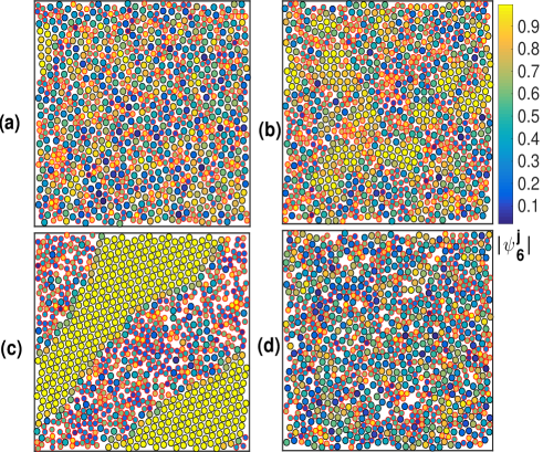
Figure 3: Steady-state configurations of the active-passive binary mixture at $n_{b}^{fcs}=$ 4 and $f_{a}=$ 3.0 at persistence times $\tau_{p}=$ 0.1 (a), $\tau_{p}=$ 0.3 (b), $\tau_{p}=$ 3.0 (c), and $\tau_{p}=$ 15.0 (d). Black (large) and red (small) edge spheres correspond to the $A$ and $B$ particles. Face color of the particles is according to the color bar for local hexatic order parameter, $|\psi_{6}^{j}|$.

III.2 Phase separation observables

The configurations of the active-passive mixture show that the system phase separates at the intermediate $\tau_{p}$ and the hexatic order increases consisting of large particles. To quantify the phase separation, we divide the simulation box into a number of square cells ($N_{cell}=8\times 8$) and calculate the difference in the number of $A$ and $B$ particles, which can be obtained by choosing the cell length, $l_{c}=$ 5.38 (along each spatial direction of the box length, $L$), for this study. The difference in the number of $A$ and $B$ particles is calculated as

$$\Phi(f_{a},\tau_{p})=\frac{1}{N_{cell}}\left\langle\sum_{i=1}^{N_{cell}}\frac{|n_{A}^{i}-n_{B}^{i}|}{(n_{A}^{i}+n_{B}^{i})}\right\rangle,$$ (6)

where $n_{A}^{i}$, $n_{B}^{i}$ are the number of $A$ and $B$ particles in an $i$th cell, respectively Chari et al. (2019). In Eq. 6, angular bracket denotes that the average is taken over the $N_{cell}$ and the steady state configurations of the system. The $\Phi(f_{a},\tau_{p})$ estimates mixing or demixing of $A$ and $B$ particles in the system: if a value of the $\Phi(f_{a},\tau_{p})$ is smaller than its critical value, then the system will be in the mixed state, and if $\Phi(f_{a},\tau_{p})$ is larger than its critical value, then the system will be in the demixed state. Hence, we consider it as a phase separation order parameter for this study.

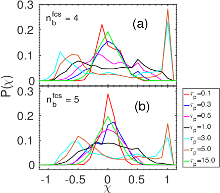
Figure 4: Probability distribution of disparity in the number of $A$ and $B$ particles, $P(\chi)$, at $f_{a}=$ 3.0, averaged over the square cells and the steady-state configurations of the system. (a) $n_{b}^{fcs}=$ 4 and (b) $n_{b}^{fcs}=$ 5.

Onset of the phase separation is considered at a critical value of the $\Phi(f_{a},\tau_{p})$, denoted by $\Phi_{c}(f_{a},\tau_{p})$ for this study. To obtain the $\Phi_{c}(f_{a},\tau_{p})$ at activity $f_{a}$ and persistence time $\tau_{p}$, we compute disparity in the number of $A$ and $B$ particles in each cell, which is calculated as $\chi=(n_{A}^{i}-n_{B}^{i})/(n_{A}^{i}+n_{B}^{i})$ over the steady states of the system Chari et al. (2019); the division of the simulation box into square cells is described above. Then, we compute distribution of $\chi$ as $P(\chi)$, which is shown in Fig. 4(a) and Fig. 4(b) for $n_{b}^{fcs}=$ 4 and 5, respectively. Figure 4(a) depicts that $P(\chi)$ has a single larger peak around $\chi=$ 0 at $\tau_{p}=$ 0.1, its height starts decreasing as the $\tau_{p}$ increases at $f_{a}=$ 3. The decrease in the peak height of the $P(\chi)$ accompanies with its broadening that splits into two peaks at intermediate persistence times. The broadening in $P(\chi)$ starts from $\tau_{p}=$ 0.3 and $f_{a}=$ 3 of $n_{b}^{fcs}=$ 4 [see Fig. 4(a)], therefore, we consider the value of $\Phi(f_{a},\tau_{p})$ at $\tau_{p}=$ 0.3 as the onset value of the phase separation order parameter, and that is $\Phi_{c}(f_{a},\tau_{p})=$ 0.3. Bimodality due to the splitting of the main peak in $P(\chi)$ is a clear sign of the disparity in the number of $A$ and $B$ particles in the square cells, and thus the signature of the phase separation. As the $\tau_{p}$ increases further, both peaks in Fig. 4(a) grow, and extent to the phase separation is shown (for example) at $\tau_{p}=$ 3 and 5 of $f_{a}=$ 3, where both peaks in $P(\chi)$ separate completely and their height also increases. From $\tau_{p}=$ 10 onwards, both peaks of $P(\chi)$ start merging again, resulting in the single peak that exhibits the mixing of active and passive particles. For $n_{b}^{fcs}=$ 5 [see Fig. 4(b)], the bimodality in $P(\chi)$ starts at the higher $\tau_{p}$ than that for $n_{b}^{fcs}=$ 4, and the extent of phase separation is reduced because of the smaller $\rho_{ab}$, which in turn reduces the peak height of $P(\chi)$ at $\tau_{p}=$ 3 and 5. This system attains $\Phi_{c}(f_{a},\tau_{p})=$ 0.3, at the higher $\tau_{p}$ that is at $\tau_{p}=$ 0.5, where demixing starts in the system for the $n_{b}^{fcs}=$ 5. Thus, the extent to the phase separation is related to the number density of the active $B$ particles in this study.

To look at finite-size effects on the phase separation, we calculate the $P(\chi)$ for $N=$ 2000 and 3000 particles; the procedure to compute $P(\chi)$ is the same as explained above. Figure 5 shows that the phase separation in the larger systems also starts at the same persistence time of the activity, which is examined from the broadening and splitting of the main peak of the $P(\chi)$ as in the case of $N=$ 1000 particles system. Figure 5 shows that the broadening in the $P(\chi)$ is more pronounced for the larger systems as compared to the $N=$ 1000 particles system, as size of domains due to the phase separation are different in the larger size systems compared to the smaller system at the same phase separation state points.

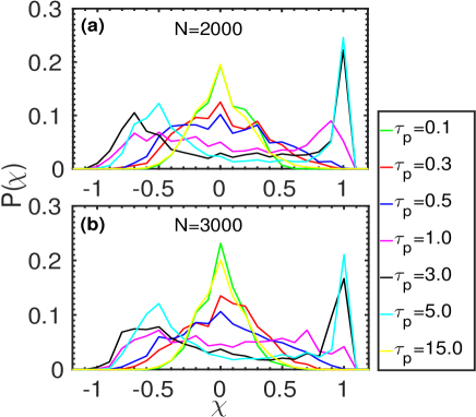
Figure 5: Probability distribution, $P(\chi)$, at $f_{a}=$ 3.0 and local neighboring threshold $n_{b}^{fcs}=$ 4, averaged over the square cells and the steady-state configurations of the system. (a) $N=$ 2000 and (b) $N=$ 3000 particles.

Further, the onset of the phase separation is also examined from the traditional correlation function that is the static structure factor Hansen and McDonald (2006), which is calculated as

$$S_{\alpha\beta}(k)=\frac{1}{N}\left\langle\sum_{i=1}^{N_{\alpha}}\sum_{j=1}^{N_{\beta}}\exp[-i\boldsymbol{k}.(\boldsymbol{r}_{j}-\boldsymbol{r}_{i})]\right\rangle,$$ (7)

where $\boldsymbol{k}$ is a wave vector and $(\alpha,\beta)\in(A,B)$; the smallest wave number is given as $k=2\pi/L$. Here, we calculate structure factor of the $A$ and $B$ particles at $f_{a}=$ 3.0 and $n_{b}^{fcs}=$ 4 with varying persistence times, which is shown in Fig. 6. Structure factors of $A$ and $B$ particles are denoted by $S_{AA}(k)$ and $S_{BB}(k)$, respectively. Figures 6(a) and 6(b) depict a growth in low wave number peak of $S_{AA}(k)$ and $S_{BB}(k)$, starting from the $\tau_{p}=$ 0.3. This growth in the peak of $S_{AA}(k)$ and $S_{BB}(k)$ at low $k$ is more pronounced at $\tau_{p}=$ 3.0 and 5.0, which corresponds to the extent of the phase separation as examined from the splitting of the main peak of the $P(\chi)$ in two peaks [see Fig. 4(a)]. The growth in the peak of $S_{AA}(k)$ and $S_{BB}(k)$, at the low wave numbers, is fitted with the Porod’s law Porod (1982) of the form $S(k)\propto k^{-3}$ at $\tau_{p}=$ 1.0, 3.0, and 5.0, which is a signature of the phase separation in the system Furukawa (1985). At $\tau_{p}=$ 15.0, the low $k$ peaks in $S_{AA}(k)$ and $S_{BB}(k)$ vanishes, which correspond to the continuous mixed state of the active-passive mixture, as evidenced by the single peak in the $P(\chi)$ [see Fig. 4(a)]. Thus, our analysis of the phase separation from the $P(\chi)$ is corroborated by the growth of the low wave number peaks in the structure factor of $A$ and $B$ particles.

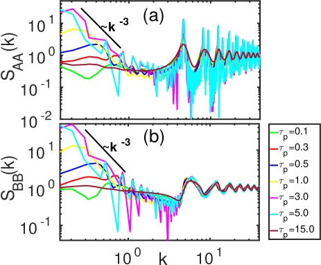
Figure 6: Static structure factor of (a) large and (b) small particles at the activity $f_{a}=$ 3.0 and $n_{b}^{fcs}=$ 4. $S_{AA}(k)$ and $S_{BB}(k)$ is fitted with the Porod’s law Porod (1982) of the form $S(k)\propto k^{-d-1}$ (see black lines) at $\tau_{p}=$ 1.0, 3.0 and 5.0. Here, $d$ ($=$ 2) is the dimensionality of the system. The growth at low wave numbers in $S_{AA}(k)$ and $S_{BB}(k)$ is a signature of phase separation in the system Furukawa (1985).

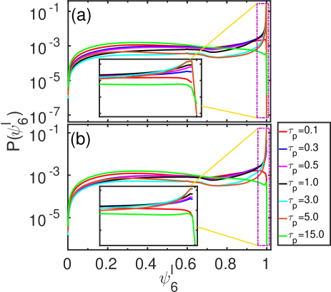
Figure 7: Probability distribution of local hexatic order, $P(\psi_{6}^{l})$, at $f_{a}=$ 3.0 and persistence times $\tau_{p}=$ 0.1-15.0. (a) $n_{b}^{fcs}=$ 4 and (b) $n_{b}^{fcs}=$ 5. The insets in (a) and (b) show the zoomed (dash-dotted) area of $P(\psi_{6}^{l})$ at $\psi_{6}^{l}=0.96-$ 1.0 .

As we know from the configurations (shown in Fig. 3) that phase separation in the system coincides with the local hexatic ordering in $A$ particles. Therefore, we look at a distribution of local hexatic ordering, averaged over the steady-state configurations of the system. Distribution of single-particle hexatic order parameter for $A$ (large) particles, $P(\psi_{6}^{l})$, is shown in Figs. 7(a) and 7(b) at $n_{b}^{fcs}=$ 4 and 5, respectively. Figure 7(a) shows that $P(\psi_{6}^{l})$ exhibits a peak near $\psi^{l}_{6}\simeq$ 1, which increases with the persistence time of the active force up to $\tau_{p}=$ 5.0, at activity $f_{a}=$ 3.0. The peak in $P(\psi_{6}^{l})$ is higher at $\tau_{p}=$ 3.0 and 5.0, where the active-passive mixture shows the extent of the phase separation. From $\tau_{p}=$ 10 onwards, the peak of $P(\psi_{6}^{l})$ near $\psi^{l}_{6}\simeq$ 1 start decreasing, showing smaller values of $P(\psi_{6}^{l})$ than that at $\tau_{p}=$ 0.1. This is because, at the higher $\tau_{p}$, the system prefers mixing and the hexatic order of majority of the particles decrease [see Fig. 3(d)], which is also supported by the merging of double peaks of $P(\chi)$ into the single peak from $\tau_{p}=$ 10 onwards [see Fig. 4(a) and Fig. 4(b)]. At $n_{b}^{fcs}=$ 5 [see Fig. 7(b)], $P(\psi_{6}^{l})$ is qualitatively similar to what found at $n_{b}^{fcs}=$ 4, only the extent to the orientational ordering in $A$ particles is smaller because the number density of the active $B$ particles reduces. On comparing the $P(\psi_{6}^{l})$ with the $P(\chi)$ at $f_{a}=$ 3, we show that the increment in the phase separation coincides with the increment in the hexatic ordering in $A$ particles. Thus, the extent to the phase separation in the system, the number density of active $B$ particles, and the hexatic order in the large particles are highly correlated.

III.3 Phase diagram

Figure 8 shows a phase diagram of the active-passive binary mixture in $\tau_{p}$-$f_{a}$ plane. To identify various regimes in the phase diagram, we calculate the phase separation order parameter $\Phi(f_{a},\tau_{p})$ [see Eq. 6 for its definition] and average hexatic order parameter for the large particles $\Psi_{6}^{l}(f_{a},\tau_{p})$. An average absolute value of the hexatic order parameter is calculated as $\Psi_{6}=N_{\alpha}^{-1}\sum_{j=1}^{N_{\alpha}}|\psi_{6}^{j}|$, where $N_{\alpha}$ is the number of particles of type $\alpha\in(A,B)$ and $\psi_{6}^{j}$ is defined in Eq. 5. Figures 8(a) and 8(b) show that $\Phi(f_{a},\tau_{p})$ increases with $\tau_{p}$ up to its intermediate values at the activity $f_{a}$. Further increasing the $\tau_{p}$, the $\Phi(f_{a},\tau_{p})$ start decreasing at each activity presented in the study. As described in Sec. III.2, the phase separation is highly correlated with the hexatic orientational ordering, therefore, we compute $\Psi_{6}^{l}(f_{a},\tau_{p})$ that is shown in Figs. 8(c) and 8(d). Similar to the $\Phi(f_{a},\tau_{p})$, the $\Psi_{6}^{l}(f_{a},\tau_{p})$ also increases with the $\tau_{p}$ up to its intermediate values. Further increasing the $\tau_{p}$, $\Psi_{6}^{l}(f_{a},\tau_{p})$ decreases to even less than that its values at the smaller $\tau_{p}$. This is because the active system is in its mixed state with smaller local hexatic order at the higher $\tau_{p}$ [see Fig. 3(d)]. Thus, the phase diagram at $n_{b}^{fcs}=$ 4, shown in Fig. 8(a) and Fig. 8(c), depicts three regimes separated by the two transition lines: the bottom transition line (BTL) separates the mixed state and the phase separation regime. The top transition line (TTL) of the phase diagram separates the phase separation region and the mixed state of active-passive particles. Thus, it shows two transitions: one from mixing to demixing and another from demixing to mixing again, which is the reentrant behavior of the system. Note that the mixed state of the particles above TTL is dissimilar to the mixed state of the particles below the BTL because the former has less orientational ordering compared to the later. The points on the BTL and TTL in the phase diagram [see Figs. 8(a–d)], at each $f_{a}$ along the line of persistence time $\tau_{p}=$ 0.01-20, correspond to the $\Phi_{c}(f_{a},\tau_{p})=$ 0.3. From the phase diagram, it is evident that the growth of $\Phi$ is highly correlated with $\Psi_{6}^{l}$, up to the TTL from below. However, the $\Psi_{6}^{l}$ decreases above the TTL compared to below BTL because activity reduces the local hexatic order that can be visualized by comparing Figs. 3(a–d). Now, it is tempting to identify the phases in these three regimes of the phase diagram by computing positional and orientational correlations.

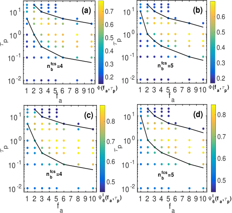
Figure 8: Phase diagram of 2D active-passive binary mixture in $\tau_{p}-f_{a}$ plane. (a–b) Order parameter of phase separation, $\Phi(f_{a},\tau_{p})$. (c–d) Average hexatic order parameter for large ($A$) particles, $\Psi_{6}^{l}(f_{a},\tau_{p})$. Black lines are corresponding to a critical value of $\Phi_{c}(f_{a},\tau_{p})=$ 0.3.

III.4 Translational and orientational order

Two-dimensional solids melt via a two-step process with the intermediate hexatic phase followed by the liquid phase. This melting occurs if volume fraction (or density) is decreased at a constant temperature, and agrees with the Kosterlitz, Thouless, Halperin, Nelson, and Young (KTHNY) two-step framework Kosterlitz and Thouless (1973); Halperin and Nelson (1978); Young (1979) in which solid to hexatic and hexatic to liquid transitions are continuous. According to the KTHNY theory, the solid phase is characterized by quasi-long-range positional order and proper long-range orientational order, whereas the hexatic phase is characterized by quasi-long-range orientational order and short-range positional order; solids show the quasi-long-range positional order in two dimensions due to the Mermin-Wagner long-wavelength fluctuations Mermin and Wagner (1966). However, studies on melting of the two-dimensional solids, consisting of repulsive hard disks Bernard and Krauth (2011) and steeply soft disks Kapfer and Krauth (2015), show solid to hexatic continuous transition and hexatic to liquid first-order transition, within the KTHNY framework. Therefore, in this study, we compute translational and orientational correlation functions to identify the phases in the three regimes of the phase diagram.

In Sec. III.2 and Sec. III.3, we have computed $P(\psi_{6}^{l})$ and $\Psi_{6}^{l}$ to examine the average local hexatic order distribution and the average hexatic order parameter for the large particles, respectively. To look at the range of this ordering, we compute hexatic order correlations as

$$g_{6}(r)=\frac{\langle\psi_{6}^{j}{\psi_{6}^{k}}^{*}\rangle|_{\mathbf{r}_{j}-\mathbf{r}_{k}=r}}{\langle|\psi_{6}^{j}|^{2}\rangle}.$$ (8)

A plot of $g_{6}^{AA}(r)$ and its fitting are displayed in Fig. 9(a) and Fig. 9(b) corresponding to $n_{b}^{fcs}=$ 4 and $n_{b}^{fcs}=$ 5, respectively. Figure 9(a) shows that the $g_{6}^{AA}(r)$ is fitted with the power law, $g_{6}^{AA}(r)\propto r^{-\eta 6}$, with an exponent $\eta 6$ that decreases continuously on increasing the $\tau_{p}$ up to $\tau_{p}=$ 5.0 at $f_{a}=$ 3.0. At the $\tau_{p}=$ 3.0 and 5.0, the exponent $\eta 6$ reaches, respectively at the values of 0.03 and 0.01 that are far smaller than 1/4, the stability limit of the hexatic phase in the continuous KTHNY transition from solid to hexatic phase. According to the KTHNY theory, there should be no decay of $g_{6}(r)$ in the solid phase that corresponds to the proper long-range orientational order. Thus, due to very small fitting exponents of the $g_{6}^{AA}(r)$ at the $\tau_{p}=$ 3.0 and 5.0, we call it a solidlike phase. On further increment in the $\tau_{p}$ at the activity $f_{a}=$ 3.0 (above the TTL) that is $\tau_{p}=$ 10.0 onwards, the $g_{6}^{AA}(r)$ decays rapidly [see Fig. 9(a)], and the exponent $\eta 6$ again increases to 2.89, though it does not fit using simple exponential that shows short-range-like orientational order in $A$ particles, corresponds to the active liquid phase; the corresponding configuration is shown in Fig. 3(d). This is because the solidlike phase melts to the hexatic that further melts to the liquid, and the orientational ordering reduces. For $n_{b}^{fcs}=$ 5 [see Fig. 9(b)], the qualitative nature of the $g_{6}^{AA}(r)$ is similar, though it differs quantitatively because the number density of the active $B$ particles is smaller that causes less phase separation. The exponents of the fitting of $g_{6}^{AA}(r)$ decrease as $\eta 6=$ 0.15 and 0.19 at the $\tau_{p}=$ 3.0 and 5.0, however, they are within the range of $0<\eta 6<1/4$, which manifests that they correspond to the (quasi-)long-range orientational order in the $A$ particles for $n_{b}^{fcs}=$ 5.

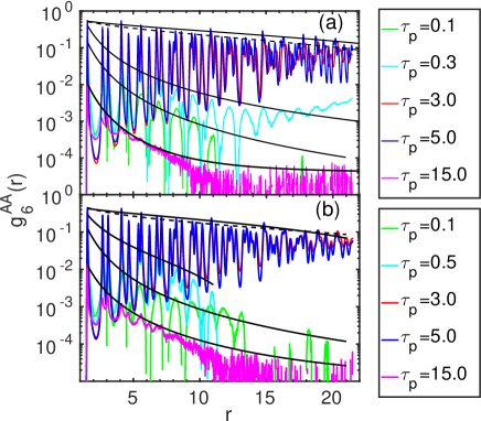
Figure 9: Hexatic order correlations in (a) at $n_{b}^{fcs}=$ 4 and (b) at $n_{b}^{fcs}=$ 5. The fitting of $g_{6}^{AA}(r)$ in (a) shows a power law $g_{6}^{AA}(r)\propto r^{-\eta 6}$ with the exponents $\eta 6=$ 2.78, 2.26, 0.035, 0.014, 2.89 at $\tau_{p}=$ 0.1, 0.3, 3.0, 5.0, 15.0, respectively. The fitting of $g_{6}^{AA}(r)$ in (b) shows the power law with exponents $\eta 6=$ 2.68, 1.53, 0.15, 0.19, 2.53 at $\tau_{p}=$ 0.1, 0.5, 3.0, 5.0, 15.0, respectively.

To look at the positional order, we compute the RDF of $A$ and $B$ particles, $g_{\alpha\beta}(r)$, defined as

$$g_{\alpha\beta}(r)=\frac{A}{2\pi r\Delta rN_{\alpha}N_{\beta}}\left\langle\sum_{i=1}^{N_{\alpha}}\sum_{\begin{subarray}{c}j=1\\ j\neq i\end{subarray}}^{N_{\beta}}\delta({r-|\mathbf{r}_{j}-\mathbf{r}_{i}|})\right\rangle,$$ (9)

where $(\alpha,\beta)\in(A,B)$. The average hexatic order [see Figs. 8(c) and 8(d)], the distribution of large particles’ local hexatic order [see Fig. 7], and the configurations of the system [see Fig. 3], show that ordering in $A$ particles increases with the persistence time up to its intermediate values and start decreasing at the higher $\tau_{p}$. Therefore, we calculate RDF of $AA$ particles and look at its fitting to examine the positional order comprising $A$ particles in the system. Figures 10(a) and 10(b) show $g_{AA}(r)$ and its fitting for $n_{b}^{fcs}=$ 4 and 5, respectively. The $g_{AA}(r)$ is fitted with the power law of the form $g_{AA}(r)\propto r^{-\eta}$ at the $\tau_{p}=$ 3.0 and 5.0 that are corresponding to the extent of the phase separation in the system at $f_{a}=$ 3.0. The obtained exponents are $\eta=$ 1.42 and 1.31 that are far larger than 1/3, the stability limit of the solid phase in the KTHNY continuous transition. However, the positional correlations decay exponentially in the hexatic phase, according to the KTHNY theory. Therefore, we consider the power-law decay of the $g_{AA}(r)$ like the quasi-long-range positional order consisting of $A$ (passive) particles. Thus, the passive $A$ particles are the solidlike at $\tau_{p}=$ 3.0 and 5.0 of $f_{a}=$ 3.0. The extent of the phase separation in the system coincides with the phase separation of the solidlike phase consisting of only passive $A$ particles, as shown in Fig. 3(c) for visualization. Figure 11(a) shows the RDF of $AA$ particles at the activity $f_{a}=$ 3.0 to look at the variation of positional order with persistence time in the range of $\tau_{p}=$ 0.1-15.0. The micro-structure of the passive (large) particles becomes rich with the increase in $\tau_{p}$ till the formation of the solidlike phase (see RDF of Fig. 10). This is because the peaks in $g_{AA}(r)$ split with increment in their height and become sharper. Thus, the RDF of $AA$ particles show that the positional order comprising $A$ particles grows from the short-range order (at smaller $\tau_{p}$) to the quasi-long-range order like at the intermediate $\tau_{p}$ of the active force. Further increase in the $\tau_{p}$, reduces the positional order in the $A$ particles, which is due to the melting of the solidlike phase into the hexatic phase that further melts to the liquid phase.

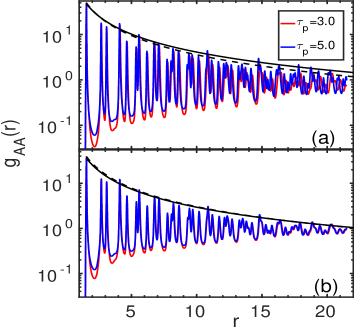
Figure 10: Radial distribution function of large particles in (a) $n_{b}^{fcs}=$ 4 and (b) $n_{b}^{fcs}=$ 5. The $g_{AA}(r)$ is fitted with the power law of the form, $g_{AA}(r)\propto r^{-\eta}$, which shows (quasi-)long-range positional order.

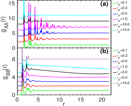
Figure 11: RDF of (a) $AA$ and (b) $BB$ particles at $f_{a}=$ 3.0 for $n_{b}^{fcs}=$ 4. In (a) and (b) plots are shifted by 2.0 and 1.0 along the $y-$axis for visibility, respectively.

Now, we look at the structural changes in the $B$ particles (active and passive) of the binary mixture with the application of activity. The RDF of $BB$ particles [see Fig. 11(b)] shows the reduction in its micro-structure as the $\tau_{p}$ is increased from the passive limit ($f_{a}=$ 0) of the activity, till the TTL is reached. The micro-structures comprising $B$ particles are considered as the splitting of the secondary peak of $g_{BB}(r)$ Kob and Anderson (1995), which start merging with increment in the $\tau_{p}$ [see Fig. 11(b)]. Interestingly, the merging of secondary peaks’ split in $g_{BB}(r)$ coincides with the increase in the positional ordering in $g_{AA}(r)$. At $\tau_{p}=$ 3.0 and 5.0 of the activity $f_{a}=$ 3.0, where the passive particles comprise the solidlike phase, height of the peaks in the $g_{BB}(r)$ [see Fig. 11(b)] decreases with $r$ up to $r=$ 4.0 that oscillates around $g_{BB}(r)=$ 2.0. The $g_{BB}(r)$ goes below 1.0 at longer distances, showing the phase separation of $A$ and $B$ particles, where $B$ particles are phase separated from the solidlike phase consisting of only $A$ particles. This coexistence region is consisting of small ($B$) and few large particles. Above TTL, the secondary peak split in $g_{BB}(r)$ reappears, shows mixing of the particles in the active liquid phase. Thus, the RDF of $A$ and $B$ particles show that the positional ordering increases in $A$ particles, whereas it decreases in $B$ particles, up to the intermediate $\tau_{p}$ (below TTL). Above TTL, both $A$- and $B$-type particles show only short-range positional ordering, and the system is in the liquid phase.

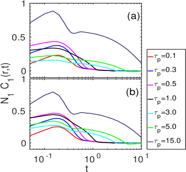
Figure 12: Velocity cross-correlations ($B-A$) within the first coordination shell at the persistence times $\tau_{p}=$ 0.1-15.0 at $f_{a}=$ 3.0. (a) $n_{b}^{fcs}=$ 4 and (b) $n_{b}^{fcs}=$ 5.

Thus, we have identified three regimes, namely, active glass (below BTL), active liquid (above TTL), and the phase separation (between the BTL and TTL) regimes by two order parameters: one is the phase separation order parameter $\Phi(f_{a},\tau_{p})$ and another is the average hexatic orientational order parameter of the large particles, $\Psi_{6}^{l}(f_{a},\tau_{p})$. The solidlike, hexatic, and liquid phases are identified by the radial distribution functions and hexatic order correlations function. However, the active glass is identified by looking at the relaxation dynamics of the system, presented in the Appendix B.

III.5 Velocity cross correlations

The QS active particles inject energy into the system that induces the transition from the active glass (mixed state) to the solid-liquid phase coexistence to the active liquid (mixed state) phases. To look at the reentrant in the orientational ordering of the system, with the persistence time of the active force, we calculate velocity cross correlations Balucani et al. (1981); Verdaguer and Padr$\acute{o}$ (2001) between $B$ and $A$ particles to examine the momentum transfer between them, which is defined as

$$C_{n}(r,t)=\frac{1}{N_{n}}\frac{{\left\langle\mathbf{v}_{i}(0).\mathbf{v}_{j}(t)\right\rangle}_{n}}{\left\langle v_{i}^{2}(0)\right\rangle},$$ (10)

where $N_{n}$ are the number of particles in the $n^{th}$ coordination shell. Normalized momentum transfer within the FCS, $N_{1}C_{1}(r,t)$, is displayed in Fig. 12(a) and Fig. 12(b) at $n_{b}^{fcs}=$ 4 and 5, respectively. Figure 12(a) shows that the momentum transfer between $B$ and $A$ particles is small at smaller $\tau_{p}$, which increases with it up to $\tau_{p}=$ 0.5. This is because the activity is insufficient to break the cages of the particles at the smaller $\tau_{p}$. The transfer of momentum from $B$ to $A$ particles decreases at $\tau_{p}=$ 1.0 and 3.0, it start increasing again from $\tau_{p}=$ 5.0, though it is less than $\tau_{p}=$ 0.3. At this intermediate $\tau_{p}$, activity fluidizes the glassy $B$ particles, whereas the $A$ particles that are passive start phase separating, resulting in the (quasi-)long-range positional and long-range orientational-like ordering. At the intermediate $\tau_{p}$, activity does not destroy the ordering of the $A$ particles, instead enhance it, and the system phase separates. Figure 12(a) shows that the momentum transfer between $B$ and $A$ particles is pronounced (from and above TTL) as the peak heights of $N_{1}C_{1}(r,t)$ shoots up because the $\tau_{p}$ is large enough to destroy the ordering of the $A$ (passive) particles. Thus, the resulting phase appears as the active liquid with the mixing of $A$ and $B$ particles. At $n_{b}^{fcs}=$ 5, the $N_{1}C_{1}(r,t)$ is qualitatively similar, though the momentum transfer between $A$ and $B$ particles is smaller than the $n_{b}^{fcs}=$ 4.

IV Conclusion

We have developed a model system for the dense active systems, where the activity is introduced by the local-density-dependent quorum sensing scheme. By applying activity to the small particles in the binary colloidal mixture, the system undergoes phase separation, accompanied by the ordering, at the intermediate persistence time of the activity. Thus, the active-passive binary mixture shows a continuous growth of hexatic order consisting of passive (large) particles from its passive glassy state on increasing persistence time at a constant activity, till the formation of the solidlike phase. Further increasing the persistence time of the active force, the positional order vanishes, and the hexatic order reappears that reduces with the persistence time. Finally, we have found that the stability in the solidlike phase is due to the least momentum transfer between active and passive particles in the phase separation regime.

Appendix A Glassy features of passive system

The average hexatic ordering in the passive colloidal mixture is examined by calculating probability distribution $P(\psi_{6})$, averaged over the equilibrium configurations of the system at $T=$ 0.01. The $P(\psi_{6})$ of $B$ particles [see Fig. A.1(a)] shows a pronounced peak around $\psi_{6}=$ 0.9, which exhibits an emergence of the hexatic order. However, the $P(\psi_{6})$ of $A$ particles shows two peaks, one around $\psi_{6}=$ 0.32 and another around $\psi_{6}=$ 0.93, which manifest the smaller orientational order in $A$ particles compared to the $B$ particles because $B$ particles show a smaller hump at the low values of the $\psi_{6}$. To examine the range of hexatic orientational ordering, we compute the hexatic order correlation function $g_{6}(r)$, defined in Eq. 8, which is shown in Fig. A.1(b). The $g_{6}(r)$ is fitted with the power law of the form $g_{6}(r)\propto r^{-\eta 6}$ with the exponents $\eta 6=$ 3.2 and 2.0, respectively for $AA$ and $BB$ particles. The exponents are far larger than $1/4$, the stability limit of the hexatic phase in the KTHNY scenario. Thus, it shows that our passive binary mixture consists of medium-range hexatic order, a feature of supercooled liquids Kawasaki and Tanaka (2011); Tah et al. (2018). The smaller value of the exponent $\eta 6$ for $B$ particles compared to the $A$ particles means a larger correlation length of hexatic order for $B$ particles. Thus, the passive system shows more (local) hexatic orientational ordering for the $B$ particles compared to the $A$ particles in this system.

The hexatic orientational order found in the absence of positional order at the size ratio 1:1.4 Hamanaka and Onuki (2006), is termed as the glassy structural order by Kawasaki and Tanaka Kawasaki and Tanaka (2011). Therefore, we examine the positional order in the system, which can be obtained from the RDF given in Eq. 9 (or its Fourier transform, widely known as structure factor). Figure A.2(a) depicts the $g(r)$ of $AA$, $BB$, and $AB$ particles, which shows an absence of long-range (or quasi-long-range) positional order in the system, however there is a medium-range hexatic orientational order as shown in Figs. A.1(a) and A.1(b). This confirms that the passive binary colloidal mixture is in its amorphous state at $T=$ 0.01 and area fraction $\phi=$ 0.628.

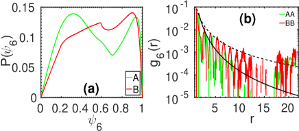
Figure A.1: (a) Probability distribution $P(\psi_{6})$ of $A$ and $B$ particles averaged over the equilibrium configurations of the passive system at $T=$ 0.01, and (b) hexatic order correlation function $g_{6}(r)$ fitted with a power law of the form, $g_{6}(r)\propto r^{-\eta 6}$; the exponent $\eta 6=$ 3.2 and 2.0 for $AA$ (solid curve) and $BB$ (dashed curve) particles.

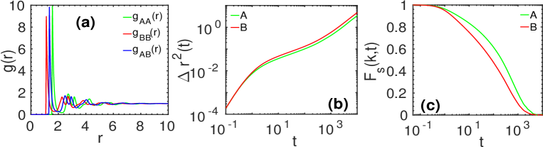
Figure A.2: Passive mixture at $T=$ 0.01 and the area fraction $\phi=$ 0.628: (a) RDFs of the binary colloidal mixture, (b) MSD of $A$ and $B$ particles, (c) incoherent intermediate scattering function, $F_{s}(k,t)$, at wave numbers corresponding to the first peak of static structure factor $S(k)$ of $A$ and $B$ particles, $k_{A}=$ 4.5 and $k_{B}=$ 5.0, respectively.

The structure of the 2D binary mixture shows that it is in the amorphous (glassy) state as described in the previous section. To confirm this, we look at the dynamics of the system. The glassy dynamics of the passive binary colloidal mixture is examined using the mean-squared displacements (MSD) and the incoherent intermediate scattering function (IISF), which are defined as

$$\Delta r^{2}(t)=\frac{1}{N}\left\langle\sum_{i=1}^{N}[\mathbf{r}_{i}(t)-\mathbf{r}_{i}(0)]^{2}\right\rangle$$ (11)

and

$$F_{s}(k,t)=\frac{1}{N}\left\langle\sum_{j=1}^{N}\exp\{i\mathbf{k}.[\mathbf{r}_{j}(t)-\mathbf{r}_{j}(0)]\}\right\rangle,$$ (12)

where wave number $k$ corresponds to the first peak of static structure factor of $A$ and $B$ particles. Here, we use $k=$ 4.5 and 5.0 for $A$ and $B$ particles, respectively. Figure A.2(b) shows the MSD of $A$ and $B$ particles at $T=$ 0.01, which exhibits a ballistic regime at short times that crossing over to the sub-diffusive regime around $t\approx$ 1.0, becomes diffusive at the longer times. The different regimes in the MSD of $A$ and $B$ particles are identified from the slope $\alpha=\partial ln\Delta r^{2}(t)/\partial lnt$ : at short times (ballistic regime) $\alpha\approx$ 2, in sub-diffusive regime $0<\alpha<1$, while in the diffusive regime $\alpha=$ 1. The sub-diffusive regime appears due to the structural cages around a tagged particle by its neighboring particles Berthier and Biroli (2011). These structural cages cause a slow down in the dynamics, thus the MSD decreases at this time scale. At long times, the particles come out of these structural cages, thus MSD again shoots up and the dynamics becomes diffusive. Although the larger ($A$) particles are slower than the smaller ($B$) ones, both sizes of particles show the sub-diffusive regime at the intermediate times [see Fig. A.2(b)], which is one of the hallmarks of the glassy dynamics Berthier and Biroli (2011). The structural relaxation of these cages is characterized using the IISF, $F_{s}(k,t)$ of both sizes of particles, which examines the relaxation of density fluctuations due to the structural cages of the particles at a wave number $k$. In this passive binary colloidal mixture, $F_{s}(k,t)$ is fitted using an empirical Kohlrausch-Williams-Watts (KWW) function of the form $f(t)^{KWW}\propto\exp(-(t/\tau)^{\beta})$, where $\beta$ is an exponent Berthier and Biroli (2011). The value of the exponent $\beta=$ 1 for the exponential density relaxations (liquid state), whereas $0<\beta<1$ for the non-exponential relaxations found in slow relaxing systems, e.g., glass-forming liquids, intracellular dynamics, motion in the crowded media, etc. For this passive binary mixture, we obtain $\beta=$ 0.66 and 0.6 for $A$ and $B$ particles, respectively. These values of $\beta$ show the non-exponential relaxation dynamics of the system at $T=$ 0.01 and area fraction $\phi=$ 0.628, which is a signature of the glassy dynamics in the passive system.

Appendix B Relaxation dynamics of the active system

Many characteristics of glassy systems are observed in the system of passive binary disks using structure and dynamics; the structure of the active system changes with the activity. As discussed in the phase diagram of the main paper, the system shows three regimes separated by the two transition lines: mixed region, phase separation, and active liquid with the mixing of both types of particles. The phase separation and the phases therein, and the active liquid are characterized in the main paper using various observables. Here, we examine the dynamics of the active-passive mixture from smaller to longer persistence times across both transition lines of the phase diagram at activity $f_{a}=$ 3.0.

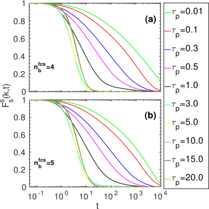
Figure A.3: Incoherent intermediate scattering function $F_{s}^{s}(k,t)$ of the small particles at $f_{a}=$ 3.0 : (a) $n_{b}^{fcs}=$ 4 and (b) $n_{b}^{fcs}=$ 5. Relaxation of the $F_{s}^{s}(k,t)$ becomes faster with increment in the $\tau_{p}$.

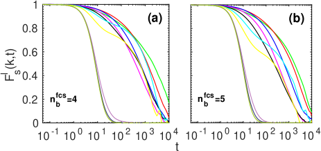
Figure A.4: Incoherent intermediate scattering function $F_{s}^{l}(k,t)$ of the large particles at $f_{a}=$ 3.0 : (a) $n_{b}^{fcs}=$ 4 and (b) $n_{b}^{fcs}=$ 5. Line colors are according to the legend of Fig. A.3. Relaxation of the $F_{s}^{l}(k,t)$ is non-monotonic with the $\tau_{p}$.

To characterize the relaxation dynamics of the active-passive mixture, we invoke incoherent intermediate scattering function. The dynamics of the system is analyzed by computing the $F_{s}(k,t)$ of $A$ and $B$ particles at the wave numbers $k=$ 4.5 and 5.0, respectively; the definition of $F_{s}(k,t)$ is given in Eq. 12. Figures A.3 and A.4 show $F_{s}(k,t)$ of $B$ and $A$ particles, respectively, at the activity $f_{a}=$ 3.0 and $\tau_{p}=$ 0.01-20 for the local neighbor threshold values $n_{b}^{fcs}=$ 4 and 5. On comparing $F_{s}(k,t)$ of passive $B$ particles [see Fig. A.2(c)] with the active $B$ particles (in Fig. A.3), it is evident that the density relaxation in the active-passive mixture becomes slower at the smaller $\tau_{p}$ because the $F_{s}(k,t)$ of passive $B$ particles relax to zero near $t\simeq 5\times 10^{3}$, whereas the $F_{s}(k,t)$ of $B$ particles in active system is above zero even till the time $t=10^{4}$. Interestingly, the $F_{s}(k,t)$ of $A$ and $B$ particles in the active system shows more slowing down for $n_{b}^{fcs}=$ 4 compared to the $n_{b}^{fcs}=$ 5 at smaller $\tau_{p}$. This slowing down is because the number density of active $B$ particles is more in case of $n_{b}^{fcs}=$ 4, showing that activity enhances the glassiness in the system at smaller $\tau_{p}$. At $f_{a}=$ 3.0, as the persistence time of active force increases (near the TTL), $F_{s}^{s}(k,t)$ shows the faster density relaxations similar to the liquids, which is due to the activity induced fluidization in the system. Thus, our system is showing the non-monotonous characteristic of the active dense systems at smaller $\tau_{p}$ (from its passive limit), as reported in a recent experimental Klongvessa et al. (2019) and simulation Berthier et al. (2017, 2019) studies of dense active colloidal systems.

At smaller $\tau_{p}$, $F_{s}^{l}(k,t)$ is qualitatively similar to the $F_{s}^{s}(k,t)$. On the other hand, the density relaxations of the $A$ particles (shown in Fig. A.4) exhibit a contrasting behavior at the intermediate $\tau_{p}$, where the system phase separates into the hexatic-liquid and solid-liquid phases. The slowing down of the $F_{s}^{l}(k,t)$ at the intermediate $\tau_{p}$ is because of the solidification that hinders the movement of the $A$ particles, enormously, and the hump in the $F_{s}^{l}(k,t)$ becomes pronounced. At $\tau_{p}=$ 3.0 and 5.0, where the active system shows the extent of the phase separation at $f_{a}=$ 3.0, it shows the glasslike density relaxations Berthier and Biroli (2011). This is because all the $A$ particles are not in the phase separation region, though, few of the $A$ particles are mixed with the $B$ particles that are in the phase coexistence region. The mixing of the $A$ and $B$ particles can be visualized from the configurations given in Fig. 3(c). Thus, our structural analysis is supporting the dynamics of the two-dimensional active-passive binary mixture in its steady state.

References

- Ramaswamy (2010) S. Ramaswamy, Ann. Rev. Condens. Matter Phys. 1, 323 (2010).
- Bechinger et al. (2016) C. Bechinger, R. D. Leonardo, H. Lwen, C. Reichhardt, G. Volpe, and G. Volpe, Rev. Mod. Phys. 88, 045006 (2016).
- Guidobaldi et al. (2014) A. Guidobaldi, Y. Jeyaram, I. Berdakin, V. V. Moshchalkov, C. A. Condat, V. I. Marconi, L. Giojalas, and A. V. Silhanek, Phys. Rev. E 89, 032720 (2014).
- Krause and Ruxton (2002) J. Krause and G. D. Ruxton, Living in Groups (Oxford University Press, Oxford, 2002).
- Berg and Turner (1979) H. C. Berg and L. Turner, Nature (London) 278, 349 (1979).
- Papenfort and Bassler (2016) K. Papenfort and B. L. Bassler, Nat. Rev. Microbiol 14, 576 (2016).
- Li et al. (2017) J. Li, B. E.-F. de vila, W. Gao, L. Zhang, and J. Wang, Sci. Robot. 2, eaam6431 (2017).
- Buerle et al. (2018) T. Buerle, A. Fischer, T. Speck, and C. Bechinger, Nature Comm. 9, 3232 (2018).
- Whiteley et al. (2017) M. Whiteley, S. P. Diggle, and E. P. Greenberg, Nature (London) 551, 313 (2017).
- Jung et al. (2015) S. A. Jung, C. A. Chapman, and W.-L. Ng, PLoS Pathog. 11, e1004837 (2015).
- Parry et al. (2014) B. R. Parry, I. V. Surovtsev, M. T. Cabeen, C. S. Hern, E. R. Dufresne, and C. Jacobs-Wagner, Cell 156, 183 (2014).
- Janssen (2019) L. M. C. Janssen, J. Phys.: Condens. Matter 31, 503002 (2019).
- Berthier and Biroli (2011) L. Berthier and G. Biroli, Rev. Mod. Phys. 83, 587 (2011).
- Klongvessa et al. (2019) N. Klongvessa, F. Ginot, C. Ybert, C. Cottin-Bizonne, and M. Leocmach, Phys. Rev. E 100, 062603 (2019).
- Berthier et al. (2017) L. Berthier, E. Flenner, and G. Szamel, New J. Phys. 19, 125006 (2017).
- Berthier et al. (2019) L. Berthier, E. Flenner, and G. Szamel, J. Chem. Phys. 150, 200901 (2019).
- Mandal et al. (2016) R. Mandal, P. J. Bhuyan, M. Rao, and C. Dasgupta, Soft Matter 12, 6268 (2016).
- Strom et al. (2017) A. R. Strom, A. V. Emelyanov, M. Mir, D. V. Fyodorov, X. Darzacq, and G. H. Karpen, Nature (London) 547, 241 (2017).
- Stenhammar et al. (2015) J. Stenhammar, R. Wittkowski, D. Marenduzzo, and M. E. Cates, Phys. Rev. Lett. 114, 018301 (2015).
- Cugliandolo et al. (2017) L. F. Cugliandolo, P. Digregorio, G. Gonnella, and A. Suma, Phys. Rev. Lett. 119, 268002 (2017).
- Geyer et al. (2019) D. Geyer, D. Martin, J. Tailleur, and D. Bartolo, Phys. Rev. X 9, 031043 (2019).
- Hamanaka and Onuki (2006) T. Hamanaka and A. Onuki, Phys. Rev. E 74, 011506 (2006).
- Kawasaki and Tanaka (2011) T. Kawasaki and H. Tanaka, J. Phys.: Condens. Matter 23, 194121 (2011).
- Hansen and McDonald (2006) J. P. Hansen and I. R. McDonald, Theory of Simple Liquids (Academic Press, London, 2006).
- Vanden-Eijnden and Ciccotti (2006) E. Vanden-Eijnden and G. Ciccotti, Chem. Phys. Lett. 429, 310 (2006).
- Binder et al. (2002) K. Binder, S. Sengupta, and P. Nielaba, J. Phys.: Condens. Matter 14, 2323 (2002).
- Chari et al. (2019) S. S. N. Chari, C. Dasgupta, and P. K. Maiti, Soft Matter 15, 7275 (2019).
- Porod (1982) G. Porod, in Small-Angle X-Ray Scattering, edited by O. Glatter and O. Kratky (Academic Press, New York, 1982).
- Furukawa (1985) H. Furukawa, Adv. Phys. 34, 703 (1985).
- Kosterlitz and Thouless (1973) J. M. Kosterlitz and D. J. Thouless, J. Phys. C: Solid State Physics 6, 1181 (1973).
- Halperin and Nelson (1978) B. I. Halperin and D. R. Nelson, Phys. Rev. Lett. 41, 121 (1978).
- Young (1979) A. P. Young, Phys. Rev. B 19, 1855 (1979).
- Mermin and Wagner (1966) N. D. Mermin and H. Wagner, Phys. Rev. Lett. 17, 1133 (1966).
- Bernard and Krauth (2011) E. P. Bernard and W. Krauth, Phys. Rev. Lett. 107, 155704 (2011).
- Kapfer and Krauth (2015) S. C. Kapfer and W. Krauth, Phys. Rev. Lett. 114, 035702 (2015).
- Kob and Anderson (1995) W. Kob and H. C. Anderson, Phys. Rev. E 51, 4626 (1995).
- Balucani et al. (1981) U. Balucani, R. Vallauri, and C. S. Murthy, Phys. Lett. 84A, 133 (1981).
- Verdaguer and Padr (2001) A. Verdaguer and J. A. Padr, J. Chem. Phys. 114, 2738 (2001).
- Tah et al. (2018) I. Tah, S. Sengupta, S. Sastry, C. Dasgupta, and S. Karmakar, Phys. Rev. Lett. 121, 085703 (2018).