A 3D Tight-Binding Model for La-Based Cuprate Superconductors

Abstract

Motivated by the recent experimental determination of the three-dimensional Fermi surface of overdoped La-based cuprate superconductors [Horio et al., Phys. Rev. Lett. ${\bf 2018}$, 121, 077004], we revisit the tight-binding parameterization of their conduction band. We construct a minimal tight-binding model entailing eight orbitals, two of them involving apical oxygen ions. Parameter optimization allows to almost perfectly reproduce the three-dimensional conduction band as obtained from density functional theory (DFT). We discuss how each parameter entering this multiband model influences it, and show that the peculiar form of its dispersion severely constraints the parameter values. We then evidence that standard perturbative derivation of an effective one-band model is poorly converging because of the comparatively small value of the charge transfer gap. Yet, this allows us to unravel the microscopical origin of the in-plane and out-of-plane hopping amplitudes. An alternative approach to the computation of the tight-binding parameters of the effective model is presented and worked out. It results that the agreement with DFT is preserved provided longer-ranged hopping amplitudes are retained. A comparison with existing models is also performed. Finally, the Fermi surface, showing staggered pieces alternating in size and shape, is compared to experiment, with the density of states also being calculated.

1 Introduction

Transition metal oxides entail a large diversity of functional oriented properties: high-T_c superconductivity [1, 2, 3, 4, 5, 6], colossal magnetoresistance observed in the manganites [7, 8, 9, 10], and transparent conducting oxides [11, 12]. In addition, a whole series of promising materials for thermoelectric applications has been discovered [13, 14, 15, 16, 17, 18, 19]. Furthermore, they also harbor fascinating phenomena such as superconductivity at the interface of two insulators [20], and peculiar metal-to-insulator transitions in vanadium sesquioxide [21, 22, 23, 24], all of them providing a strong challenge to study these systems from the theory side. Such a task implies the derivation of an appropriate microscopical model containing the relevant degrees of freedom. To some extend, the least degree of complexity arises when modeling the superconducting cuprates as, in that case, only one band crosses the Fermi energy. Accordingly, the Hubbard model on the square lattice is often considered as the proper low energy effective model of the superconducting cuprates[25]. It has been studied by a whole range of approaches, but it remains fair to say that a widely accepted theory of the cuprates, and more generally of strongly correlated oxides, is still to come.

In an effort to set up a generic model applicable to most superconducting cuprates, P. W. Anderson suggested to focus on the CuO₂ layers that are common to these materials, and, accordingly, to simplify the one-body term of the Hamiltonian down to nearest-neighbor hopping on the square lattice formed by the Cu ions [25]. He further suggested to assume a fully screened Coulomb interaction that only retains the local (Hubbard) interaction term among the $d_{x^{2}-y^{2}}$ electrons that form the only band crossing the Fermi energy. Intense efforts devoted to study the resulting two-dimensional (2D) Hubbard model has shown that it captures the basic phenomenology of the cuprates[26, 27, 28]. However, these endeavors did not allow to systematically yield long-ranged pure d-wave pairing order in the hole doped region of interest (from the underdoped $\delta\simeq$ 5$\%$ region to the overdoped $\delta\simeq$ 27$\%$ one with $\delta$ the hole doping in a half-filled band). In addition, the so-called 1/8 anomaly is found to be related to a magnetic stripe. Yet, the period of the calculated one is twice larger than experimentally observed [29, 30, 31]. Eventually, this failure may originate from an oversimplification of the model, and it has been suggested that including hopping to the next-nearest neighbors (with hopping amplitude $t^{\prime}$) leads to the correct stripe periodicity[32, 30, 33, 34]. Therefore, the physics entailed in the Hubbard model is sensitive to the very form of its one-body term. This is even more so since recent calculations indicate that the role of $t^{\prime}$ is to suppress d-wave pairing correlations[33]. This, however, is in contrast to the DFT study by Pavarini et al. [35], who showed that a larger $t^{\prime}$ is empirically correlated to a higher maximal T_c in each family of cuprate compounds. The role of possible longer-ranged hopping terms, and their relationship with oxygen orbitals, received a lesser degree of attention.

Irrespective of the form of the interaction ultimately leading to superconductivity, the one-body term of the Hamiltonian is of interest on its own, for several reasons. First, from the experimental point of view it has been established long ago that the superconducting transition temperature T_c is quite sensitive to the very structure of a sample, that is primarily reflected in the hopping term. For instance, the critical temperature is 25 K in bulk La_1.9Sr_0.1CuO₄[36], while T_c reaches 49 K in thin film form[37, 38]. Second, knowing the proper parameter set entering the kinetic energy term of the Hamiltonian might be helpful when performing numerical simulations, in particular when tackling effective low energy Hamiltonians such as the one-band Hubbard model. Alternatively, one may wonder whether the rather weak exotic superconductivity found in the repulsive $t-U$ Hubbard model[39, 40, 27, 33] persists when further hopping terms are taken into account. Third, it is of interest to understand the microscopic origin of the various hopping amplitudes entering the kinetic energy of the effective model. How do effective models based on “in layer only” CuO₂ orbitals compare to models taking the third dimension into account? Fourth, the reduction of multiband models down to an effective one-band model often results from a perturbative treatment. Yet, the relative proximity of the Cu:3d${}_{x^{2}-y^{2}}$ and O:2p energy levels prevents this treatment from being rapidly converging, and an alternative procedure to this downfolding procedure might be precious. Fifth, the Fermi surface of La_1.78Sr_0.22CuO₄ as measured by Horio et al. [41] is not to be interpreted within a Hubbard model on the square lattice.

In this work, we therefore propose to re-examine the influence of the oxygen ions, including the apical ones, on the electronic structure with a particular emphasis on the form of the inter-layer couplings. More specifically, we take the single-layer La-based cuprate superconductors La_2-xSr_xCuO₄ (LSCO) as examples [1]. Their layered body-centered tetragonal structure (BCT) [42] is explicitely taken into account. In this context, we neglect all Cu:3d orbitals but the 3d${}_{x^{2}-y^{2}}$ one, so that the underlying effective low-energy model still consists of a one-band Hubbard model, but because of the BCT structure, we retain the six relevant O:2p orbitals that shape the conduction band. The often advocated Cu:4s orbital is incorporated in our model, too [43, 35, 44, 45, 46].

The paper is organized as follows: we shortly review existing microscopical models in Section 2. We set up a three-dimensional eight-band tight-binding model in Section 3 where we show that all included orbitals have a sizeable influence on the dispersion of the conduction band. We also argue that the other oxygen orbitals may be safely neglected. In Section 4, we start the discussion by giving a set of optimized parameters which yields an almost perfect agreement with DFT results by Markiewicz et al. [47]. We then address downfolding procedures to derive an effective one-band model. We first show that the perturbative treatment to fifth order does not show sign of convergence to the exact result for realistic values of the charge transfer gap. However, this allows us to qualitatively discuss the different higher order superexchange processes contributing to the effective hopping integrals. The latter are then numerically computed by means of the Fourier transform of the exact conduction band. Finally, we discuss the peculiar calculated Fermi surface of the 3D model which is compared to the recent experimental results by Horio et al. [41]. The density of states is addressed as well. The paper is summarized and concluded in Section 5.

2 Emery and related microscopical models

Below, we propose a starting point to the description of the low-energy physics of superconducting La-based cuprates (La₂CuO₄ as parent compound). This model goes beyond the popular three-band tight-binding Emery model [48, 49, 50] which we summarize below, as it will serve as a basis for comparison. Since it is based on a single CuO₂ layer, it entails no dispersion in the direction perpendicular to them, in contrast to DFT calculations that are performed for the 3D compounds [47, 51].

In real space, the one-body term describing an ideal CuO₂ layer reads:

$$\hat{H}_{\rm E}^{(0)}=\epsilon_{d}\sum_{{\bf i},\sigma}\hat{n}_{{\bf i},\sigma}^{d}+\epsilon_{p}\left(\sum_{{\bf j},\sigma}\hat{n}^{(X)}_{{\bf j},\sigma}+\sum_{{\bf l},\sigma}\hat{n}^{(Y)}_{{\bf l},\sigma}\right)+\hat{T}_{pd}+\hat{T}_{pp}\,,$$ (1)

with

$$\hat{T}_{pd} =t_{pd}\sum_{{\bf i},\sigma}\hat{d}_{{\bf i},\sigma}^{\dagger}\left(\hat{p}_{x,{\bf i}+\frac{a}{2}{\bf e_{x}},\sigma}^{(X)}-\hat{p}_{x,{\bf i}-\frac{a}{2}{\bf e_{x}},\sigma}^{(X)}-\hat{p}_{y,{\bf i}+\frac{a}{2}{\bf e_{y}},\sigma}^{(Y)}\right.$$ (2)

$$\left.+\hat{p}_{y,{\bf i}-\frac{a}{2}{\bf e_{y}},\sigma}^{(Y)}\right)+h.c.\,\,{\rm and}\,,$$

$$\hat{T}_{pp} =t_{pp}\sum_{{\bf i},\sigma}\hat{p}_{x,{\bf i}+\frac{a}{2}{\bf e_{x}},\sigma}^{(X)\dagger}\left(\hat{p}_{y,{\bf i}-\frac{a}{2}{\bf e_{y}},\sigma}^{(Y)}-\hat{p}_{y,{\bf i}+\frac{a}{2}{\bf e_{y}},\sigma}^{(Y)}\right)$$

$$+\hat{p}_{x,{\bf i}-\frac{a}{2}{\bf e_{x}},\sigma}^{(X)\dagger}\left(\hat{p}_{y,{\bf i}+\frac{a}{2}{\bf e_{y}},\sigma}^{(Y)}-\hat{p}_{y,{\bf i}-\frac{a}{2}{\bf e_{y}},\sigma}^{(Y)}\right)+h.c.\,,$$

where ${\bf i}\equiv{\bf R}_{i}$ is the position of the Cu site in the CuO₂ plaquette of the Bravais lattice. The lattice parameter $a$ is the shortest Cu-Cu distance, and $\hat{d}^{\dagger}_{{\bf i},\sigma}$ is the creation operator of an electron with the spin $\sigma$ = $\left(\uparrow,\downarrow\right)$ on the Cu:3d${}_{x^{2}-y^{2}}$ orbital on site ${\bf i}$ with on-site energy $\epsilon_{d}$ and occupation number operator $\hat{n}_{{\bf i},\sigma}^{d}$. Two O:2p oxygen orbitals are embodied in the model through the $\hat{p}_{x,{\bf j},\sigma}^{(X)\dagger}$ (${\bf j}\equiv{\bf R}_{i}+a{\bf e}_{x}/2$), and $\hat{p}_{y,{\bf l},\sigma}^{(Y)\dagger}$ (${\bf l}\equiv{\bf R}_{i}+a{\bf e}_{y}/2$) creation operators. The on-site oxygen energy is $\epsilon_{p}$ with the occupation number operators $\hat{n}^{(X)}_{{\bf j},\sigma}$ and $\hat{n}^{(Y)}_{{\bf l},\sigma}$. The kinetic part of the Hamiltonian Eq. (2) refers to the hopping amplitude $t_{pd}=\langle 3d_{x^{2}-y^{2},{\bf i}}|\hat{T}_{pd}|p_{x,{\bf i}+a{\bf e}_{x}/2}^{(X)}\rangle$ = $-\langle 3d_{x^{2}-y^{2}}|\hat{T}_{pd}|p_{y,{\bf i}+a{\bf e}_{y}/2}^{(Y)}\rangle$ between the 2p${}_{x}^{(X)}$ and 2p${}_{y}^{(Y)}$ oxygen orbitals and the 3d${}_{x^{2}-y^{2}}$ orbital, and the hopping amplitude between both oxygen orbitals given by $t_{pp}=-\langle p_{x,{\bf i}+a{\bf e}_{x}/2}^{(X)}|\hat{T}_{pp}|p_{y,{\bf i}+a{\bf e}_{y}/2}^{(Y)}\rangle$. The form of the kinetic part of the Emery model is better known in momentum space. Applying the Fourier transform on Eqs. (1) and (2), the non-interacting Emery three-band Hamiltonian in momentum space is given by:

$$\hat{H}_{\rm E}^{(0)}=\sum_{{\bf k},\sigma}\hat{\Phi}_{{\bf k},\sigma}^{\dagger}\begin{pmatrix}\epsilon_{d}&2it_{pd}p_{x}&-2it_{pd}p_{y}\\ -2it_{pd}p_{x}&\epsilon_{p}&-4t_{pp}p_{x}p_{y}\\ 2it_{pd}p_{y}&-4t_{pp}p_{x}p_{y}&\epsilon_{p}\end{pmatrix}\hat{\Phi}_{{\bf k},\sigma}$$ (3)

with

$$p_{x}\equiv\sin{\left(\frac{k_{x}a}{2}\right)}\>\>,\>\>p_{y}\equiv\sin{\left(\frac{k_{y}a}{2}\right)}\,.$$ (4)

Here, all creation operators of electrons on Cu:3d and O:2p orbitals with the momentum ${\bf k}$ and spin $\sigma$ are gathered in the three-component operator $\hat{\Phi}_{{\bf k},\sigma}^{\dagger}=\left(\hat{d}_{{\bf k},\sigma}^{\dagger},\hat{p}_{x,{\bf k},\sigma}^{(X)\dagger},\right.$ $\left.\hat{p}_{y,{\bf k},\sigma}^{(Y)\dagger}\right)$. Consensus about the value of the parameters does not seem to have been reached but typical values in t_pd unit are given by: $\epsilon_{d}-\epsilon_{p}\simeq 2.5-3.5t_{pd}$ and $t_{pp}\simeq 0.5-0.6t_{pd}$, with $t_{pd}\simeq 1.2-1.5$ eV[52, 48, 53, 54, 55, 2, 56, 35, 57].

Since a realistic non-interacting Hamiltonian which can be implemented in quantum correlated treatments is crucial in order to correctly describe the unconventional properties of the superconducting cuprates [4, 58], other models have been put forward. For instance, a generic 2D four-band model for CuO₂ planes was suggested by Labbé and Bok[59]. Later, Andersen et al. [43] derived a 2D 8-band model extending the Emery model which interpolates the LDA band structure of stoichiometric YBa₂Cu₃O₇. They thereby showed that the shape of the Fermi surface is entirely characterized by the in-plane hopping parameters $t$, $t^{\prime}\simeq-0.30t$ and $t^{\prime\prime}\simeq 0.20t$. In order to shed light on their DFT results for LSCO, Markiewicz et al. [47] introduced a phenomenological effective model. Using, $E_{3D}(k_{x},k_{y},k_{z})=\epsilon_{M}+E_{2D}(k_{x},k_{y})+E_{z}(k_{x},k_{y},k_{z})$ the purely 2D contribution reads:

$$\begin{split}E_{2D}(k_{x},k_{y})=-2t\left[\cos{(k_{x}a)}+\cos{(k_{y}a)}\right]\\ -4t^{\prime}\cos{(k_{x}a)}\cos{(k_{y}a)}\\ -2t^{\prime\prime}\left[\cos{(2k_{x}a)}+\cos{(2k_{y}a)}\right]\\ -4t^{\prime\prime\prime}\left[\cos{(k_{x}a)}\cos{(2k_{y}a)}+\cos{(k_{y}a)}\cos{(2k_{x}a)}\right]\,,\end{split}$$ (5)

where $t$, $t^{\prime}$, $t^{\prime\prime}$ and $t^{\prime\prime\prime}$ represent first, second, third and fourth nearest-neighbor in-plane hopping integrals. Regarding the out-of-plane dispersion Markiewicz et al. entangle all three space dimensions using:

$$E_{z}(k_{x},k_{y},k_{z})=-2t_{z}\pi_{x}\pi_{y}\pi_{z}\left[\cos{(k_{x}a)}-\cos{(k_{y}a)}\right]^{2}$$ (6)

where

$$\pi_{x}\equiv\cos{(k_{x}a/2)}\>\>,\>\>\pi_{y}\equiv\cos{(k_{y}a/2)}\>\>,\>\>\pi_{z}\equiv\cos{(k_{z}c/2)}\,,$$ (7)

and $t_{z}$ denotes an inter-layer hopping parameter. The offset by (a/2, a/2) of the successive CuO₂ layers is taken into account through the factor $\pi_{x}\pi_{y}$ [47]. The constant $\epsilon_{M}$ makes $E_{3D}(0,0,0)$ vanishing. This model has also been used in order to fit the experimental out-of-plane Fermi surface of overdoped LSCO ($\delta$ = 0.22) obtained with ARPES [41]. In addition, a three-dimensional (3D) four-band tight-binding model was derived by Mishonov et al.[45] in order to explain the observation of the 3D Fermi surface in Tl₂Ba₂CuO_6+δ[60].

3 Extended three-dimensional model

The goal of this section is to set up a tight-binding model for La-based cuprates. More specifically we attempt to reproduce the dispersion of the band based on the Cu:3d${}_{x^{2}-y^{2}}$ orbital along the main symmetry lines of the Brillouin zone, including the ouf-of-plane ones, as obtained by DFT calculations by Markiewicz et al.[47]. There is an extensive literature on copper orbitals that may play an important role to high-T_c superconductivity (HTSC) [2, 3, 61]. It has predominantly been focused on the 3d${}_{x^{2}-y^{2}}$, 3d${}_{3z^{2}-r^{2}}$, and 4s orbitals that are closest to the Fermi energy [43, 62, 35, 58, 63]. The assumption that some form of the one-band Hubbard model harbors the key ingredient to HTSC leads to neglect the 3d${}_{3z^{2}-r^{2}}$ (filled) orbital altogether, as it may not be simply integrated out because of the strong interaction of these electrons with the ones populating the 3d${}_{x^{2}-y^{2}}$ orbitals. In other words, keeping both e_g orbitals unavoidably results in a two-band Hubbard model [64, 63]. Since the interaction of the latter electrons with the 4s electrons is much weaker, integrating out the latter is better justified and we explicitly take them into account in our tight-binding model, as proposed in Refs. [43, 35].

We start the construction of our model by considering the four inequivalent oxygen ions building octahedra surrounding a given copper atom: there are two in-plane oxygen ions O^(X) and O^(Y) along the x and y directions respectively and two apical oxygens O^(a) and O^(b), located above and below each copper ion, respectively. This leads to twelve nearly degenerate O:2p orbitals to be considered. Yet, as will be addressed below, only six of them significantly contribute to the dispersion of the Cu:3d${}_{x^{2}-y^{2}}$ band. Structure wise, the numerical value of the lattice parameters is given by: $a=b=3.78\leavevmode\nobreak\$Å and $c=13.18\leavevmode\nobreak\$Å. The position of the copper site and the oxygen sites in a unit-cell $i$ are given by ${\bf R}_{Cu}={\bf R}_{i}$, ${\bf R}_{O^{(X)}}={\bf R}_{i}+a{\bf e}_{x}/2$, ${\bf R}_{O^{(Y)}}={\bf R}_{i}+a{\bf e}_{y}/2$, ${\bf R}_{O^{(a)}}={\bf R}_{i}+d_{\rm Cu-O_{ap}}{\bf e}_{z}$ and ${\bf R}_{O^{(b)}}={\bf R}_{i}-d_{\rm Cu-O_{ap}}{\bf e}_{z}$. The distance $r\equiv d_{\rm Cu-O_{ap}}=2.42\leavevmode\nobreak\$Å$=0.64a$ characterizes the elongation of the octahedra. Let us observe here that symmetry forces a whole series of hopping amplitudes to vanish. In particular one has:

$$\langle 3d_{x^{2}-y^{2}}|\hat{T}|p_{z}^{(X,Y)}\rangle=\langle 3d_{x^{2}-y^{2}}|\hat{T}|p_{x,y}^{(a,b)}\rangle=0$$ (8)

and

$$\langle 4s|\hat{T}|p_{z}^{(X,Y)}\rangle=\langle 4s|\hat{T}|p_{x,y}^{(a,b)}\rangle=0.$$ (9)

Hence those six oxygen orbitals do at best play a minor role and are therefore neglected. Accordingly, all along this work we consider the eight orbitals: Cu:3d${}_{x^{2}-y^{2}}$, Cu:4s, $O^{(X)}:2p_{x}^{(X)}$, $O^{(Y)}:2p_{y}^{(Y)}$, $O^{(X)}:2p_{y}^{(X)}$, $O^{(Y)}:2p_{x}^{(Y)}$, $O^{(a)}:2p_{z}^{(a)}$, $O^{(b)}:2p_{z}^{(b)}$, in this order. Further arguments for this choice can be found in Refs. [35, 43, 65, 66, 67, 68, 69, 70, 71]. These eight orbitals are labeled by an index $\mu$ that runs from 1 to 8. Subsets of orbitals involving all of them but the Cu:3d${}_{x^{2}-y^{2}}$ one are labeled by an index $\nu$ that runs from 2 to 8, subsets of orbitals involving the in-plane oxygen orbitals are labeled by an index $\kappa$ running from 3 to 6, while the subset of apical oxygen orbitals is labeled by $\rho$ that runs from 7 to 8. Our eight-band tight-binding Hamiltonian may be expressed as:

$$\mathcal{\hat{H}}_{\rm(8)}=\hat{H}_{0}+\hat{T}+\hat{H}_{d},$$ (10)

where $\hat{H}_{0}$ stands for the on-site orbital energies relative to $\epsilon_{d}$ which denotes the on-site energy of the 3d${}_{x^{2}-y^{2}}$ orbital and $\hat{T}$ is the kinetic energy term. Introducing the Fourier transform $\hat{d}_{\bf k,\sigma}$ of the annihilation operator of an electron on site $i$ with spin $\sigma$ on the 3d${}_{x^{2}-y^{2}}$ orbital:

$$\hat{d}_{{\bf k},\sigma}=\frac{1}{\sqrt{L}}\sum_{{\bf k},\sigma}e^{-i{\bf k}\cdot{\bf R}_{i}}\hat{d}_{i,\sigma}\,,$$ (11)

and analogous expressions for the other orbitals, $\hat{H}_{0}$ reads:

$$\hat{H}_{0}=\sum_{{\bf k},\sigma}\left[-\Delta_{pd}\sum_{\kappa}\hat{n}_{{\bf k},\sigma,\kappa}^{p}-\Delta_{z}\sum_{\rho}\hat{n}_{{\bf k},\sigma,\rho}^{p_{z}}+\Delta_{s}\hat{n}_{{\bf k},\sigma}^{s}\right]\,,$$ (12)

where $\Delta_{pd}=\epsilon_{d}-\epsilon_{p}$, $\Delta_{z}=\epsilon_{d}-\epsilon_{z}$, $\Delta_{s}=\epsilon_{s}-\epsilon_{d}$. Additionally, $\epsilon_{p}$, $\epsilon_{z}$ and $\epsilon_{s}$, denote the on-site energies of the 2p${}_{x,y}^{(X,Y)}$, 2p_z and Cu:4s orbitals, respectively. The various $\hat{n}_{{\bf k},\sigma,\mu}$ operators represent the occupation number operators of a given orbital with momentum ${\bf k}$ and spin $\sigma$. L is the size of the lattice. Gathering all creation operators in the eight-component operator $\hat{\Psi}_{{\bf k},\sigma,\mu}^{\dagger}$ = $\left(\hat{d}_{{\bf k},\sigma}^{\dagger}\right.$, $\hat{s}_{{\bf k},\sigma}^{\dagger}$, $\hat{p}_{x,{\bf k},\sigma}^{(X)\dagger}$, $\hat{p}_{y,{\bf k},\sigma}^{(Y)\dagger}$, $\hat{p}_{y,{\bf k},\sigma}^{(X)\dagger}$, $\hat{p}_{x,{\bf k},\sigma}^{(Y)\dagger}$, $\hat{p}_{z,{\bf k},\sigma}^{(a)\dagger}$, $\left.\hat{p}_{z,{\bf k},\sigma}^{(b)\dagger}\right)$, the kinetic energy may be written as:

$$\hat{T}=\sum_{{\bf k},\sigma}\sum_{\mu,\mu^{\prime}}t_{\bf k}^{\mu,\mu^{\prime}}\hat{\Psi}_{{\bf k},\sigma,\mu}^{\dagger}\hat{\Psi}_{{\bf k},\sigma,\mu^{\prime}}^{\phantom{\dagger}}\,.$$ (13)

Here $t_{\bf k}^{\mu,\mu^{\prime}}$ is the hopping integral in momentum space between orbital $\mu$ and orbital $\mu^{\prime}$. Finally, we have

$$\hat{H}_{d}=\epsilon_{d}\sum_{{\bf k},\sigma}\sum_{\mu}\hat{\Psi}_{{\bf k},\sigma,\mu}^{\dagger}\hat{\Psi}_{{\bf k},\sigma,\mu}^{\phantom{\dagger}}\,.$$ (14)

Altogether, we focus on the one-body Hamiltonian

$$\hat{\mathcal{H}}=\hat{H}_{0}+\hat{T}$$ (15)

expressed as:

$$\mathcal{\hat{H}}=\sum_{{\bf k},\sigma}\sum_{\mu,\mu^{\prime}}\hat{\Psi}_{{\bf k},\sigma,\mu}^{\dagger}H_{\bf k}^{\mu,\mu^{\prime}}\hat{\Psi}_{{\bf k},\sigma,\mu^{\prime}}^{\phantom{\dagger}}\,,$$ (16)

with

$$H_{{\bf k}}=\begin{pmatrix}A_{{\bf k}_{\parallel}}&B_{{\bf k}_{\parallel}}&C_{k_{z}}\\ B_{{\bf k}_{\parallel}}^{\dagger}&D_{{\bf k}_{\parallel}}&E_{{\bf k}}\\ C_{k_{z}}^{\dagger}&E_{{\bf k}}^{\dagger}&F_{{\bf k}}\end{pmatrix}\,.\>\>\>\>\>\>\>\>\$$ (17)

Here, the Hamiltonian matrix is expressed in terms of the sub-matrices A${}_{{\bf k}_{\parallel}}$, D${}_{{\bf k}_{\parallel}}$ and F_k entailing the tight-binding Hamiltonians in the copper, in-plane oxygen, and out-of-plane oxygen orbital subspaces, respectively. The coupling between these subspaces is accounted for by the submatrices B${}_{{\bf k}_{\parallel}}$, C${}_{k_{z}}$ and E_k. While the Hamiltonian matrix Eq. (17) depends on the momentum ${\bf k}=({\bf k}_{\parallel},k_{z})$, we clarified the momentum dependence of the sub-matrices, that are derived below.

3.1 In-plane hopping integrals

In this sub-section, we set up the contribution to the Hamiltonian arising from the copper and in-plane oxygen orbitals. This leads to a two-dimensional model. The positions in the unit-cell $i$ of the O^(X) and O^(Y) ions are respectively labeled by ${\bf j}\equiv{\bf R}_{i}+a{\bf e}_{x}/2$ and ${\bf l}\equiv{\bf R}_{i}+a{\bf e}_{y}/2$.

3.1.1 Oxygen - copper and direct copper - copper hopping integrals

The strong d-p $\sigma$-hybridization has already been presented in Section 2. Then, in agreement with arguments given in Refs. [35, 43] we include in the model the effect of the Cu:4s orbital. It strongly hybridizes with the nearest neighboring O^(X):2p${}_{x}^{(X)}$ and O^(Y):2p${}_{y}^{(Y)}$ orbitals. They are located at relative positions $\pm a{\bf e}_{x}/2$ and $\pm a{\bf e}_{y}/2$ and the corresponding hopping matrix elements are $\pm t_{sp}=\langle 4s_{\bf i}|\hat{T}|p_{x,{\bf i}\pm a{\bf e}_{x}/2}^{(X)}\rangle$. Symmetry implies that $\pm t_{sp}=\langle 4s_{\bf i}|\hat{T}|p_{y,{\bf i}\pm a{\bf e}_{y}/2}^{(Y)}\rangle$. Note that the matrix elements of the kinetic energy between the Cu:4s orbital and the remaining O^(X) and O^(Y) orbitals vanish. Since the Cu:4s orbital is more extended than the 3d one we also include direct nearest neighbor 4s-4s hopping amplitude $-t_{ss}$ = $\langle 4s_{\bf i}|\hat{T}|4s_{{\bf i}\pm a{\bf e}_{x}}\rangle$ and the next nearest neighbor one $-t_{ss}^{\prime}$ = $\langle 4s_{\bf i}|\hat{T}|4s_{{\bf i}\pm a({\bf e}_{x}+{\bf e}_{y})}\rangle$, together with their symmetry related counterparts. The matrices $A_{{\bf k}_{\parallel}}$ and $B_{{\bf k}_{\parallel}}$ then follow as:

$$A_{{\bf k}_{\parallel}}=\bordermatrix{\leavevmode\nobreak\ &{|3d_{x^{2}-y^{2}}\rangle}&{|4s\rangle}\cr&0&0\cr&0&\tilde{\Delta}_{{\bf k}_{\parallel}}\cr}\,,$$ (18)

where we introduced the short-hand notation:

$$\tilde{\Delta}_{{\bf k}_{\parallel}}=\Delta_{s} -2t_{ss}(\cos{(k_{x}a)}+\cos{(k_{y}a}))$$ (19)

$$-4t_{ss}^{\prime}\cos{(k_{x}a)}\cos{(k_{y}a)}\,,$$

and

$$B_{{\bf k}_{\parallel}}=\bordermatrix{\leavevmode\nobreak\ &{|p_{x}^{(X)}\rangle}&{|p_{y}^{(Y)}\rangle}&{|p_{y}^{(X)}\rangle}&{|p_{x}^{(Y)}\rangle}\cr&2it_{pd}p_{x}&-2it_{pd}p_{y}&0&0\cr&2it_{sp}p_{x}&2it_{sp}p_{y}&0&0\cr}\,.$$ (20)

The matrix B${}_{{\bf k}_{\parallel}}$ accounts for the coupling between the Cu (3d and 4s) orbitals and the involved in-plane oxygen one. With the above sign convention $t_{pd}$, $t_{sp}$, $t_{ss}$ and $t^{\prime}_{ss}$ are all positive.

3.1.2 Oxygen-Oxygen hopping integrals

a) Neighboring oxygen ions along the axes of the square lattice

We first consider the hopping integrals between the in-plane 2p${}_{x,y}^{(X,Y)}$ oxygen orbitals. While the ionic radius of Cu²⁺ is commonly accepted to be close to $0.75\leavevmode\nobreak\$Å, the one of O^2- is $1.35\leavevmode\nobreak\$Å, which results into a strong hybridization of the oxygen orbitals among themselves. Indeed, the diameter of the O^2- ions is comparable to the distance between nearest-neighbors O^(X) and O^(Y) oxygen ions on a CuO₂ plaquette given by $a/\sqrt{2}$ = 2.68 Å. We thus introduce the $\sigma$-type hopping integral between nearest-neighbor 2p${}_{x}^{(X)}$ orbitals, $t_{\sigma^{\prime}}$ = $\langle p_{x,{\bf j}}^{(X)}|\hat{T}|p_{x,{\bf j}\pm a{\bf e_{x}}}^{(X)}\rangle$ as depicted in Fig. 1. Similarly, $t_{\sigma^{\prime}}$ = $\langle p_{y,{\bf j}}^{(X)}|\hat{T}|p_{y,{\bf j}\pm a{\bf e_{y}}}^{(X)}\rangle$ is the hopping amplitude between nearest-neighbor 2p${}_{y}^{(X)}$ orbitals. Likewise, for symmetry reasons, $\langle p_{y,{\bf l}}^{(Y)}|\hat{T}|p_{y,{\bf l}\pm a{\bf e_{y}}}^{(Y)}\rangle$ and $\langle p_{x,{\bf l}}^{(Y)}|\hat{T}|p_{x,{\bf l}\pm a{\bf e_{x}}}^{(Y)}\rangle$ will be given by $t_{\sigma^{\prime}}$ as well. In addition, $\pi$-type coupling between two O^(X) neighbors linked along $\pm a{\bf e_{y}}$ and $\pm a{\bf e_{x}}$ are also considered. They are both accounted for by the hopping integral $-t_{\pi^{\prime}}$ = $\langle p_{x,{\bf j}}^{(X)}|\hat{T}|p_{x,{\bf j}\pm a{\bf e_{y}}}^{(X)}\rangle$ = $\langle p_{y,{\bf j}}^{(X)}|\hat{T}|p_{y,{\bf j}\pm a{\bf e_{x}}}^{(X)}\rangle$. Symmetry implies that the $\pi$-type hopping integrals involving the oxygen O^(Y) ions are again given by $-t_{\pi^{\prime}}$ = $\langle p_{x,{\bf l}}^{(Y)}|\hat{T}|p_{x,{\bf l}\pm a{\bf e_{y}}}^{(Y)}\rangle$ = $\langle p_{y,{\bf l}}^{(Y)}|\hat{T}|p_{y,{\bf l}\pm a{\bf e_{x}}}^{(Y)}\rangle$. With the above used sign conventions, $t_{\sigma^{\prime}}$ and $t_{\pi^{\prime}}$ are positive. Furthermore symmetry forces all matrix elements $\langle p^{(X,Y)}_{x,y,{\bf j}}|\hat{T}|p^{(X,Y)}_{z,{\bf j}}\rangle$ to vanish.

b) Neighboring oxygen ions along the diagonal axis of the square lattice

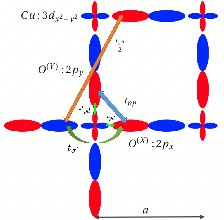
Figure 1: (Color online) Illustration of $t_{pd}$, $t_{\sigma^{\prime}}$, $t_{pp}$ and $t_{\sigma^{\prime\prime}}$ in-plane hopping amplitudes. Note that t_pp = $(t_{\sigma}+t_{\pi})/2$ and $t_{\sigma^{\prime\prime}}$ are introduced using the rotated orbital basis (2p${}_{\xi}^{(X,Y)}$, 2p${}_{\eta}^{(X,Y)}$).

In order to introduce the $\sigma$- and $\pi$-type hopping matrix elements between nearest-neighbor O^(X) and O^(Y) ions we take advantage of a transformation consisting in a rotation by $\pi/4$ around ${\bf e}_{z}$ of the 2$p_{x,y}^{(X,Y)}$ orbitals for each given oxygen site. It leads to define $\hat{p}_{\xi}^{(\beta)}=(\hat{p}_{x}^{(\beta)}+\hat{p}_{y}^{(\beta)})/\sqrt{2}$ and $\hat{p}_{\eta}^{(\beta)}=(-\hat{p}_{x}^{(\beta)}+\hat{p}_{y}^{(\beta)})/\sqrt{2}$ where $\beta\in(X,Y)$. With this transformation we obtain an alternative (or rotated) 2p oxygen orbital basis in which $\sigma$- and $\pi$-hybridization along the diagonal directions between all oxygen ions of the lattice is easily taken into account. We thus consider hybridization between 2p${}_{\xi}^{(X)}$ and 2p${}_{\xi}^{(Y)}$ along $({\bf e}_{x}+{\bf e}_{y})/\sqrt{2}$ with the associated hopping integral $t_{\sigma}$ = $\langle p_{\xi,{\bf j}}^{(X)}|\hat{T}|p_{\xi,{\bf j}\pm a({\bf e}_{x}+{\bf e}_{y})/2}^{(Y)}\rangle$. The same hopping amplitude $t_{\sigma}$ is obtained when the 2p${}_{\eta}^{(X,Y)}$ orbitals are considered along the orthogonal direction: $t_{\sigma}$ = $\langle p_{\eta,{\bf j}}^{(X)}|\hat{T}|p_{\eta,{\bf j}\pm a({\bf e}_{x}-{\bf e}_{y})/2}^{(Y)}\rangle$. Furthermore, concerning the $\pi$-type hybridization, we have $-t_{\pi}$ = $\langle p_{\eta,{\bf j}}^{(X)}|\hat{T}|p_{\eta,{\bf j}\pm a({\bf e}_{x}+{\bf e}_{y})/2}^{(Y)}\rangle$ along $({\bf e}_{x}+{\bf e}_{y})/\sqrt{2}$ and $-t_{\pi}$ = $\langle p_{\xi,{\bf j}}^{(X)}|\hat{T}|p_{\xi,{\bf j}\pm a({\bf e}_{x}-{\bf e}_{y})/2}^{(Y)}\rangle$ along $({\bf e}_{x}-{\bf e}_{y})/\sqrt{2}$.

We also take into account, in this basis, the $\sigma$-coupling between next-nearest neighbors O^(X) and O^(Y) ions. This leads to the hopping integral $t_{\sigma^{\prime\prime}}$ = $\langle p_{\xi,{\bf w}}^{(\beta)}|\hat{T}|p_{\xi,{\bf w}\pm a({\bf e}_{x}+{\bf e}_{y})}^{(\beta)}\rangle$. Symmetry implies $t_{\sigma^{\prime\prime}}$ = $\langle p_{\eta,{\bf w}}^{(\beta)}|\hat{T}|p_{\eta,{\bf w}\pm a({\bf e}_{x}-{\bf e}_{y})}^{(\beta)}\rangle$, with ${\bf w}\in({\bf j,l})$. The corresponding $\pi$-type hopping amplitudes are clearly smaller than the $\sigma$-type ones, and may be neglected (see Fig.  1). Then the hopping amplitude between $\sigma$-type 2p:O^(X,Y) next-nearest neighbor orbitals is $t_{\sigma^{\prime\prime}}/2$ in the natural basis. The matrix D${}_{{\bf k}_{\parallel}}$ embodying the tight-binding model for the four in-plane 2p oxygen orbitals therefore results as:

$$\begin{split}D_{{\bf k}_{\parallel}}=\>\>\>\>\>\>\>\>\>\>\>\>\>\>\>\>\>\>\>\>\>\>\>\>\>\>\>\>\>\>\>\>\>\>\>\>\>\>\>\>\>\>\>\>\>\>\>\>\>\>\>\>\>\>\>\>\>\>\>\>\>\>\>\>\>\>\>\>\>\>\>\>\>\>\>\>\>\>\>\>\>\>\>\>\>\>\>\>\>\>\>\>\>\>\>\>\>\>\>\>\>\>\>\>\>\>\>\>\>\>\>\>\>\>\>\>\>\>\>\>\>\>\>\>\>\>\>\>\>\>\>\>\>\>\>\>\>\>\>\>\>\>\>\>\\ \leavevmode\resizebox{385.92152pt}{}{ $$\bordermatrix{\leavevmode\nobreak\ &{|p_{x}^{(X)}\rangle}&{|p_{y}^{(Y)}\rangle}&{|p_{y}^{(X)}\rangle}&{|p_{x}^{(Y)}\rangle}\cr&\bar{\Delta}_{{\bf k}_{\parallel}}&-4t_{pp}p_{x}p_{y}&-2t_{\sigma^{\prime\prime}}p_{2x}p_{2y}&4t_{pp}^{(2)}\pi_{x}\pi_{y}\cr&-4t_{pp}p_{x}p_{y}&\bar{\Delta}_{{\bf k}_{\parallel}}^{\prime}&4t_{pp}^{(2)}\pi_{x}\pi_{y}&-2t_{\sigma^{\prime\prime}}p_{2x}p_{2y}\cr&-2t_{\sigma^{\prime\prime}}p_{2x}p_{2y}&4t_{pp}^{(2)}\pi_{x}\pi_{y}&\bar{\Delta}_{{\bf k}_{\parallel}}^{\prime}&-4t_{pp}p_{x}p_{y}\cr&4t_{pp}^{(2)}\pi_{x}\pi_{y}&-2t_{\sigma^{\prime\prime}}p_{2x}p_{2y}&-4t_{pp}p_{x}p_{y}&\bar{\Delta}_{{\bf k}_{\parallel}}\cr}$$ }\leavevmode\nobreak\ \leavevmode\nobreak\ \leavevmode\nobreak\ \leavevmode\nobreak\ \leavevmode\nobreak\ \end{split}$$ (21)

where we have defined:

$$\begin{split}\bar{\Delta}_{{\bf k}_{\parallel}}=-\Delta_{pd}+2(t_{\sigma^{\prime}}\cos{(k_{x}a)}-t_{\pi^{\prime}}\cos{(k_{y}a)})\\ +2t_{\sigma^{\prime\prime}}\cos{(k_{x}a)}\cos{(k_{y}a)}\\ \bar{\Delta}_{{\bf k}_{\parallel}}^{\prime}=-\Delta_{pd}+2(t_{\sigma^{\prime}}\cos{(k_{y}a)}-t_{\pi^{\prime}}\cos{(k_{x}a)})\\ +2t_{\sigma^{\prime\prime}}\cos{(k_{x}a)}\cos{(k_{y}a)}\>,\end{split}$$ (22)

together with

$$t_{pp}=\frac{t_{\sigma}+t_{\pi}}{2}\>\>,\>\>t_{pp}^{(2)}=\frac{t_{\sigma}-t_{\pi}}{2}\,.$$ (23)

In addition, we introduced

$$p_{2x}\equiv\sin{(k_{x}a)}\>\>\>\>,\>\>\>\>p_{2y}\equiv\sin{(k_{y}a)}\>.$$ (24)

Furthermore, we note that $t_{pp}$ is identical to the O^(X)-O^(Y) hopping integral involved in the Emery model Eq. (3) [48]. However, the smaller hopping amplitude $t_{pp}^{(2)}$ is neglected in the Emery model. While the alternative orbital basis (2p${}_{\xi}^{(X,Y)}$, 2p${}_{\eta}^{(X,Y)}$) eases the derivation of D${}_{{\bf k}_{\parallel}}$, the latter is written in the natural basis. This completes the derivation of a two-dimensional model.

3.2 Out-of-plane hopping integrals

In this subsection we derive the main contributions leading to dispersion perpendicular to the CuO₂ layers. Because of the body-centered tetragonal structure there is no obvious leading term describing the hopping of an electron on a Cu:3d${}_{x^{2}-y^{2}}$ orbital in one layer to the same orbital on a neighboring layer. Such processes involve at least the apical oxygens through their 2p_z orbitals, which themselves couple to the Cu:4s orbital[66, 35, 69, 71] and to in-plane O:2p orbitals. With this, one can attempt to model the rather broad dispersion along $k_{z}$ found in DFT calculations[47]. Below, the position in the unit-cell of apical oxygens O^(a) and O^(b) are labeled by ${\bf m}\equiv{\bf R}_{i}+{\rm d_{Cu-O_{ap}}}{\bf e}_{z}$ and ${\bf n}\equiv{\bf R}_{i}-{\rm d_{Cu-O_{ap}}}{\bf e}_{z}$, respectively.

3.2.1 Coupling of the apical oxygen ions to the in-plane orbitals

Here, we describe the coupling of the apical oxygen ions to the copper and in-plane oxygen ions. First, the hopping amplitude associated to the Cu:4s and its nearest neighbors in ${\bf e}_{z}$ direction O^(a,b):2p_z orbitals is given by $t_{sp_{z}}=\langle p_{z,{\bf m}}^{(a)}|\hat{T}|4s_{\bf i}\rangle$ and $-t_{sp_{z}}=\langle p_{z,{\bf n}}^{(b)}|\hat{T}|4s_{\bf i}\rangle$ (as shown by the blue arrows in Fig. 2). Second, symmetry yields $\langle p_{z,{\bf i}\pm r{\bf e}_{z}}^{(a,b)}|\hat{T}|3d_{x^{2}-y^{2},{\bf i}}\rangle$ = 0. Hence, the couplings between the Cu orbitals and the 2p${}_{z}^{(a,b)}$ apical oxygen orbitals may be gathered in:

$$C_{k_{z}}=\bordermatrix{\leavevmode\nobreak\ &{|p_{z}^{(a)}\rangle}&{|p_{z}^{(b)}\rangle}\cr&0&0\cr&t_{sp_{z}}e^{irk_{z}}&-t_{sp_{z}}e^{-irk_{z}}\cr}\,.$$ (25)

In addition, the 2p${}_{z}^{(a,b)}$ apical oxygen orbitals significantly hybridize with the in-plane 2p${}_{x,y}^{(X,Y)}$ oxygen ones. Indeed, with the distance between a copper ion and an apical oxygen ion being d${}_{\rm Cu-O_{ap}}$ $\simeq 0.64a$ the distance between an apical oxygen ion and an in-plane oxygen ion in the unit-cell is d${}_{\rm O-O_{ap}}$ $\simeq 0.80a$. This is comparable to the in-plane distance d${}_{\rm O^{(X)}-O^{(Y)}}$ $\simeq 0.707a$ in the unit-cell. Then, taking the point of view of apical oxygens, the O^(a):2p${}_{z}^{(a)}$ orbital hybridizes with 2p${}_{x}^{(X)}$ orbital along $\boldsymbol{\delta}_{-}^{(\pm)}=\pm a{\bf e}_{x}/2-d_{\rm Cu-O_{ap}}{\bf e}_{z}$ with the associated hopping integral $\mp t_{p_{z}}=\langle p_{z,{\bf m}}^{(a)}|\hat{T}|p_{x,{\bf m}+\boldsymbol{\delta}_{-}^{(\pm)}}^{(X)}\rangle$ and 2p${}_{y}^{(Y)}$ along $\boldsymbol{\delta}_{-}^{\prime(\pm)}=\pm a{\bf e}_{y}/2-d_{\rm Cu-O_{ap}}{\bf e}_{z}$ with $\mp t_{p_{z}}=\langle p_{z,{\bf m}}^{(a)}|\hat{T}|p_{y,{\bf m}+\boldsymbol{\delta}_{-}^{\prime(\pm)}}^{(Y)}\rangle$. Besides, O^(b):2p${}_{z}^{(b)}$ orbital also hybridizes with 2p${}_{x}^{(X)}$ orbital along $\boldsymbol{\delta}_{+}^{(\pm)}=\pm a{\bf e}_{x}+d_{\rm Cu-O_{ap}}{\bf e}_{z}$ with the associated hopping integral $\pm t_{p_{z}}$ = $\langle p_{z,{\bf n}}^{(b)}|\hat{T}|p_{x,{\bf n}+\boldsymbol{\delta}_{+}^{(\pm)}}^{(X)}\rangle$ and 2p${}_{y}^{(Y)}$ along $\boldsymbol{\delta}_{+}^{\prime(\pm)}=\pm a{\bf e}_{y}+d_{Cu-O_{ap}}{\bf e}_{z}$ with $\pm t_{p_{z}}=\langle p_{z,{\bf n}}^{(b)}|\hat{T}|p_{y,{\bf n}+\boldsymbol{\delta}_{+}^{\prime(\pm)}}\rangle$. These couplings are illustrated in Fig. 2 by green arrows.

Furthermore, the coupling between the 2p${}_{z}^{(a,b)}$ apical orbitals (belonging to the nearest upper and lower CuO₂ layers) with in-plane 2p${}_{x}^{(Y)}$ and 2p${}_{y}^{(X)}$ orbitals should be considered, too. Below, the distance between the current CuO₂ layer and the next-layer apical oxygen ions is denoted by $v\equiv d_{\rm O_{ap}}^{\rm(next-layer)}=c/2-d_{\rm Cu-O_{ap}}\simeq 1.1a$. Let us begin with O${}^{(b)}:2p_{z}^{(b)}$ located in the upper layer at (a/2, a/2, d${}_{\rm O_{ap}}^{\rm(next-layer)}$). It hybridizes with the 2p${}_{x}^{(Y)}$ orbital. The associated hopping amplitude is $\mp t_{p_{z}}^{\prime\prime}$ = $\langle p_{z,\boldsymbol{\nu}_{+}}^{(b)}|\hat{T}|p_{x,\boldsymbol{\nu}_{+}-v{\bf e}_{z}\pm{\bf e}_{x}/2}^{(Y)}\rangle$. Here we introduced $\boldsymbol{\nu}_{\pm}$ = $a({\bf e}_{x}+{\bf e}_{y})/2\pm d_{\rm O_{ap}}^{\rm(next-layer)}{\bf e}_{z}$ the position of an O^(b) (O^(a)) ion in the upper (lower) layer relative to the Cu ion in the current layer. The next-layer $O^{(b)}$ also hybridizes with the $2p_{y}^{(X)}$ orbital with the associated hopping amplitude $\mp t_{p_{z}}^{\prime\prime}$ = $\langle p_{z,\boldsymbol{\nu}_{+}}^{(b)}|\hat{T}|p_{y,\boldsymbol{\nu}_{+}-v{\bf e}_{z}\pm{\bf e}_{y}/2}^{(X)}\rangle$. Symmetry implies that the apical oxygen O^(a):2p${}_{z}^{(a)}$ orbital belonging to the lower layer at (a/2, a/2, -d${}_{\rm O_{ap}}^{\rm(next-layer)}$) hybridizes (with opposite sign) with the in-plane 2p${}_{x}^{(Y)}$ and 2p${}_{y}^{(X)}$ orbitals. Therefore, the associated hopping integrals are $\pm t_{p_{z}}^{\prime\prime}$ = $\langle p_{z,\boldsymbol{\nu}_{-}}^{(a)}|\hat{T}|p_{x,\boldsymbol{\nu}_{-}+v{\bf e}_{z}\pm{\bf e}_{x}/2}^{(Y)}\rangle$ = $\langle p_{z,\boldsymbol{\nu}_{-}}^{(a)}|\hat{T}|p_{y,\boldsymbol{\nu}_{-}+v{\bf e}_{z}\pm{\bf e}_{y}/2}^{(X)}\rangle$. These couplings between in-plane 2p orbitals and out-of-plane 2p${}_{z}^{(a,b)}$ orbitals may be gathered in:

$$E_{\bf k}=\bordermatrix{\leavevmode\nobreak\ &{|p_{z}^{(a)}\rangle}&{|p_{z}^{(b)}\rangle}\cr&2it_{p_{z}}p_{x}e^{irk_{z}}&-2it_{p_{z}}p_{x}e^{-irk_{z}}\cr&2it_{p_{z}}p_{y}e^{irk_{z}}&-2it_{p_{z}}p_{y}e^{-irk_{z}}\cr&-2it_{p_{z}}^{\prime\prime}p_{y}e^{-ivk_{z}}&2it_{p_{z}}^{\prime\prime}p_{y}e^{ivk_{z}}\cr&-2it_{p_{z}}^{\prime\prime}p_{x}e^{-ivk_{z}}&2it_{p_{z}}^{\prime\prime}p_{x}e^{ivk_{z}}\cr}\,.$$ (26)

3.2.2 Apical oxygens - Apical oxygens hopping amplitudes

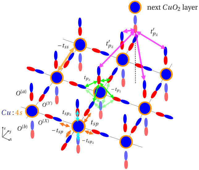
Figure 2: (Color online) Illustration of the body-centered tetragonal lattice of single-layer La-based cuprate involving the 2p${}_{x,y}^{(X,Y)}$ in-plane oxygen, 2p${}_{z}^{(a,b)}$ out-of-plane apical oxygen, and Cu:4s orbitals. The inter-layer coupling is also illustrated.

To complete the model we now proceed with the derivation of the tight-binding Hamiltonian in the out-of-plane oxygen orbital subspace. Since neither the 2p${}_{x}^{(a,b)}$ nor the 2p${}_{y}^{(a,b)}$ orbitals couple to the 3d${}_{x^{2}-y^{2}}$ and 4s copper orbitals we are left with the 2p${}_{z}^{(a,b)}$ orbitals only. Further contributions to dispersion in the direction perpendicular to CuO₂ layers come from the 2p_z orbitals of the apical oxygens. With the body-centered tetragonal symmetry of the lattice, each apical oxygen O^(a) (O^(b)) is surrounded by four nearest-neighbor apical oxygen O^(b) (O^(a)) ions belonging to the upper (lower) next CuO₂ layer. For example, we illustrate in Fig. 2 (magenta arrows) the coupling between the O^(a) apical oxygen located at (0, 0, d${}_{{\rm Cu-O_{ap}}}$) of the reference unit-cell with one of its apical nearest neighbor O^(b) located at (a/2, a/2, c/2-d${}_{{\rm Cu-O_{ap}}}$) in the unit-cell centered at (a/2, a/2, c/2). Since their distance is as small as d${}_{{\rm Cu-O_{ap}}}$, the associated hopping amplitude $t_{p_{z}}^{\prime}$ has to be taken into account. Concerning the apical oxygen O^(a) located at ${\bf m}$, the four nearest-neighbor inter-plane apical oxygens O^(b) are located at ($\pm$a/2, $\pm$a/2, d${}_{{\rm Cu-O_{ap}}}$ + d${}_{\rm O^{(a)}-O^{(b)}}$) where $u\equiv d_{\rm O^{(a)}-O^{(b)}}=c/2-2d_{\rm Cu-O_{ap}}=0.465a$ is the distance along the c-axis between two inter-plane apical oxygen ions. Thus, we introduce the corresponding hopping integrals $t_{p_{z}}^{\prime}$ = $\langle p_{z,{\bf m}}^{(a)}|\hat{T}|p_{z,{\bf m}+a(\pm{\bf e}_{x}\pm{\bf e}_{y})/2+u{\bf e}_{z}}^{(b)}\rangle$. Symmetry implies: $t_{p_{z}}^{\prime}$ = $\langle p_{z,{\bf n}}^{(b)}|\hat{T}|p_{z,{\bf n}+a(\pm{\bf e}_{x}\pm{\bf e}_{y})/2-u{\bf e}_{z}}^{(a)}\rangle$. The coupling between O^(a) and O^(b) in the unit-cell is also taken into account through $t_{p_{z}}^{\prime\prime\prime}$ = $\langle p_{z,{\bf m}}^{(a)}|\hat{T}|p_{z,{\bf n}}^{(b)}\rangle$. Note that the $\pi$-overlap between the O^(a):2p_z orbitals - and between the O^(b):2p_z orbitals - is of order $t_{\pi^{\prime\prime}}$ and may be neglected. Then, the matrix F_k which accounts for the coupling between inter-layer apical oxygen orbitals is given by:

Let us note that all previously defined tight-binding parameters are taken positive (the sign of the orbital lobes are taken care of through the adopted sign convention). Symmetry implies that many seemingly large hopping amplitudes actually vanish (see, e. g., Eqs. (8,9)). We neglected hybridizations implying the 2p${}_{z}^{(X,Y)}$ orbitals because they are smaller than the largest retained ones, so that our model is an eight-band model that may hardly be improved on in the tight-binding framework. Below, our model will be tested against the LDA results obtained by Markiewicz et al.[47], as well as against the one-band tight-binding model they use to capture their numerical findings.

4 Results and discussion

The purpose of this section is to establish an effective one-band model for Cu:3d${}_{x^{2}-y^{2}}$ band through the downfolding of the other seven bands. Because of the relatively small value of the gap between the oxygen bands and the copper one, one may infer that numerous relevant effective hopping integrals will come into play. Our procedure will hence allow for highlighting their origin in the multiband model, and for addressing what can and cannot follow from the Emery model Eq. (3).

X[5l]X[5l]X[5l]X[5l]X[5l]X[5l]X[5l]X[6l]Summary of the set of optimal tight-binding parameters in units of $t_{pd}$ fitting the LDA dispersion of the conduction band (Fig. 4). $\Delta_{pd,opt}=3.5$ & $\Delta_{z,opt}=2.6$ $\Delta_{s,opt}=6.5$ $t_{\sigma,opt}=0.95$ $t_{\sigma^{\prime},opt}=0.13$ $t_{\sigma^{\prime\prime},opt}=0.4$$t_{sp,opt}=1.3$ $t_{\pi,opt}=0.2375$
$t_{ss,opt}=0.40$ $t_{ss,opt}^{\prime}=0.10$ $t_{sp_{z},opt}=1.4$ $t_{p_{z},opt}=0.95$ $t_{p_{z},opt}^{\prime}=0.45$ $t_{p_{z},opt}^{\prime\prime}=0.10$ $t_{p_{z},opt}^{\prime\prime\prime}=0$ $t_{\pi^{\prime},opt}=0.0325$

4.1 Electronic structure and comparison to DFT

We now proceed with the dispersion of the bands resulting from the tight-binding Hamiltonian Eq. (15). In the following we focus on the path 1 connecting the symmetry points $\Gamma$=(0, 0, 0), X=($\pi/a$, 0, 0) and M=($\pi/a$, $\pi/a$, 0) as well as on the path 2 connecting the symmetry points Z=(0, 0, $2\pi/c$), R=($\pi/a$, 0, $2\pi/c$), and A=($\pi/a$, $\pi/a$, $2\pi/c$). The electronic structure of the model is shown in Fig. 3. The six lowest in energy bands have O:2p character: the four in-plane ones are lower in energy than the two out-of-plane ones. Not only do they show large dispersion along paths 1 and 2, but all six bands display strong dependence on $k_{z}$ as well. Regarding the bands originating from the Cu ions, the highest in energy one has a predominant Cu:4s character while the second highest in energy one has predominant Cu:3d${}_{x^{2}-y^{2}}$ character. On their own the former shows a weak ${\bf k}_{\parallel}$ dependence, while the latter is fully local. Hence they inheritate their dispersion from their coupling to the oxygens. The so-obtained band widths are smaller than for the oxygen based ones, but dispersion along the three directions is obtained for both Cu-based bands.

Figure 3: (Color online) Electronic structure along path 1 (full lines) and path 2 (dashed lines) arising from the eight-band tight-binding model. The used tight-binding parameters are given in Table 4.

Figure 4: (Color online) (a) Comparison of the dispersion of the conduction band as obtained within DFT by Markiewicz et al.[47] (circles) to our tight-binding model. Here, $E_{cb}(\pi/a,0,0)$ defines the zero of energy and the $k_{z}=2\pi/c$ line is shifted by 1 eV, for clarity. (b) Energy difference $\Delta E_{z}({\bf k}_{\parallel})$ Eq. (28) as a function of ${\bf k}_{\parallel}$. The used tight-binding parameters are given in Table 4, together with $t/t_{pd}=0.283$.

Let us now focus on the Cu:3d${}_{x^{2}-y^{2}}$ conduction band (the only one crossing the Fermi level), of dispersion $E_{cb}({\bf k})$. As will be discussed in sub-section 4.3, the conduction band shows strong sensitivity to the choice of the parameter set entering the Hamiltonian, not only from the point of view of the band width, but also from the point of view of the shape of the band. Hence we first stick to an optimal set of tight-binding parameters (see Table 4) which provides a good fit of the conduction band as obtained from DFT by Markiewicz et al. for the LSCO compound[47]. The dispersion of the conduction band for $k_{z}$ = 0 and $k_{z}$ = $2\pi/c$ obtained from our model is compared to a set of data points from LDA calculations [47] in Fig. 4 and Fig. 5. Regarding path 1 that encompasses the symmetry lines $\Gamma$-X-M-$\Gamma$, Figs. 4(a) and 5 demonstrate an almost perfect agreement between our model and DFT calculations. A good agreement is also found along path 2, at the exception of the vicinity of the Z point. The energy difference:

$$\Delta E_{z}({\bf k}_{\parallel})=E_{cb}({\bf k}_{\parallel},k_{z}=2\pi/c)-E_{cb}({\bf k}_{\parallel},k_{z}=0)$$ (28)

is also plotted in Fig. 4(b). Amazingly no $k_{z}$-dispersion arise above the X-M-$\Gamma$ symmetry line. It only appears above the $\Gamma$-X symmetry line (anti-nodal direction). This feature is shared by the Markiewicz 3D tight-binding model[47] (Eqs. (5, 6)) and is exhibited by LDA calculations[47, 51]. It has also been observed in recent ARPES experiments[41].

A more accurate comparison of the calculated dispersion along $\Gamma$-X to LDA is presented in Fig. 5. Clearly, the dispersion yielded by our model is in good agreement with the DFT results in the vicinity of ($\pi/a$, 0, $k_{z}$) that is close to the Fermi energy for a half-filled band. The agreement remains good for ${\bf k}$ = ($\pi/2a$, 0, $k_{z}$) but degrades when going towards the bottom of the band. In Fig. 5 we also compare the tight-binding model set up by Markiewicz et al. [47] (see Eqs. (5, 6)) to their DFT results, in which case good agreement is obtained only in the very vicinity of the ($\pi/a$, 0, $k_{z}$) symmetry line. In fact, for both models, the dispersion of the LDA conduction band along $\Gamma$-Z is poorly accounted for. At first glance this could be attributed to the neglected terms. Yet, the largest (though small) of them do not bring dispersion of the conduction band along $\Gamma$-Z, so that this rather points to a limitation of a tight-binding description that neglects other Cu orbitals. Yet, when sticking to the vicinity of half-filling, this primarily affects rather high energy excitations, which turn out to be larger than the ones involving the top of the (here neglected) 3d${}_{3z^{2}-r^{2}}$ band [72].

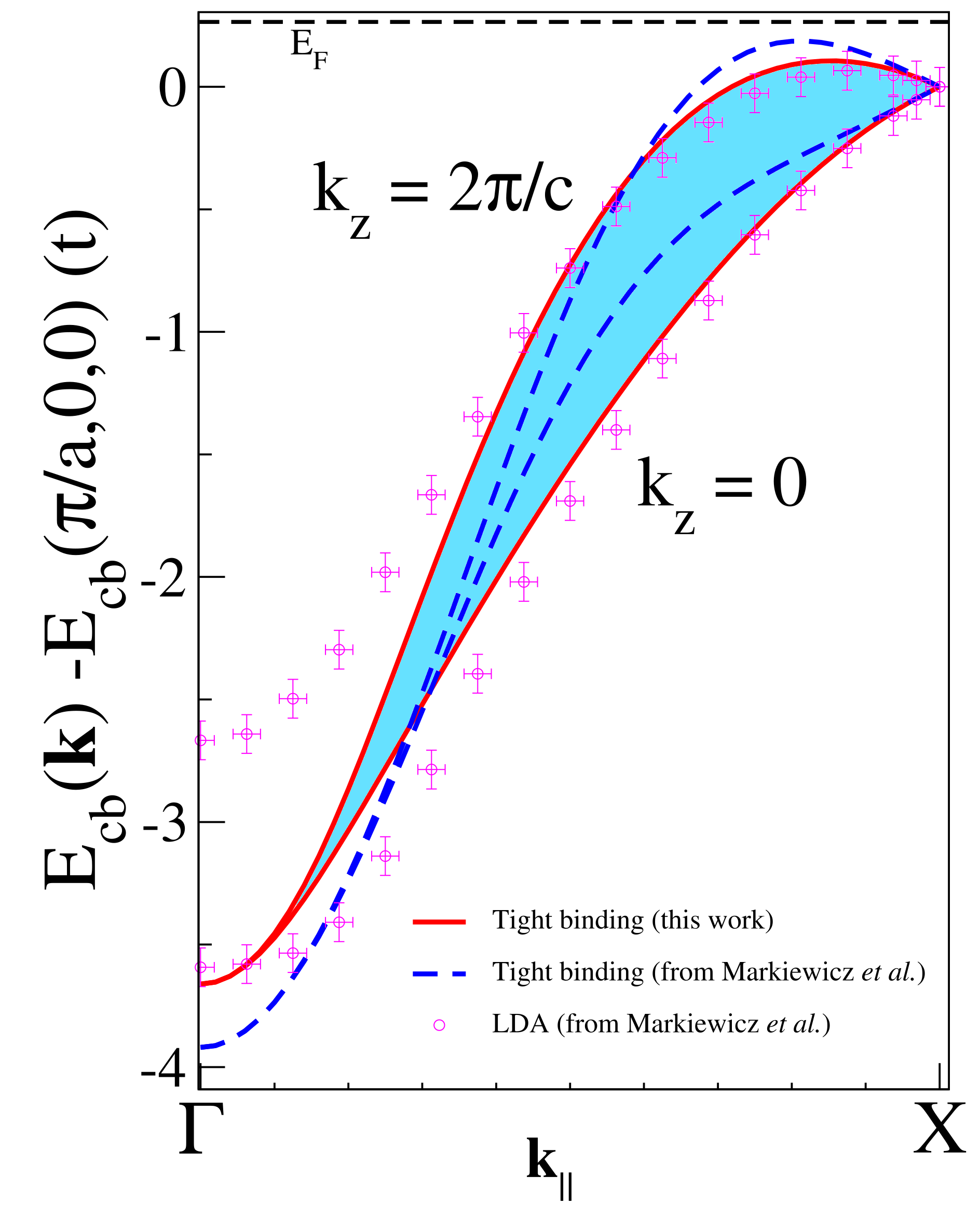
Figure 5: (Color online) Dependence on $k_{z}$ of the conduction band as a function of ${\bf k}_{\parallel}$ along $\Gamma$-X. The shaded blue region is bounded by the band for $k_{z}=0$ and $k_{z}=2\pi/c$. The used tight-binding parameters are given in Table 4, together with $t/t_{pd}=0.283$.

4.2 Analytical approach: microscopical origin of the effective hopping amplitudes from downfolding

Below, we discuss the connection between hopping processes involved in our model and within a one-band effective description of the conduction band through a downfolding of the multiband Hamiltonian Eq. (15). Indeed, as previously seen in Section 2, cuprates are often described within the Emery model[48, 49] and it was suggested that this model can be reduced to an equivalent effective single-band Mott-Hubbard system with the Zhang-Rice singlet band playing the role of the lower Hubbard band [73]. This point of view supports the early proposal by P. W. Anderson [25] that essential physics of cuprates would be captured by a one-band Hubbard-like model in which the kinetic part is made of the nearest neighbor and the next-nearest neighbor integrals $t$ and $t^{\prime}$ in addition to the local repulsive interaction that favors electron localization. However, such a description is only based on a square lattice and neglects the body-centered tetragonal structure of single-layer La-based cuprates responsible for inter-plane coupling. Here, focusing on the kinetic part of the model, we follow this route by integrating out the oxygen and the Cu:4s degrees of freedom in order to obtain a one-band effective model describing the conduction band. The one-band Hamiltonian has the ${\bf k}$ dependence of a Fourier series. Then, the copper band expression for the dispersion has an in-plane part E${}_{\parallel}({\bf k}_{\parallel})$ and an inter-plane part E${}_{z}({\bf k})$, which, up to a constant ensuring $E(0)=0$, reads:

$$E({\bf k}_{\parallel},k_{z})=E_{\parallel}(k_{x},k_{y})+E_{z}(k_{x},k_{y},k_{z})=\frac{1}{L}\sum_{i,j}t_{i,j}e^{i{\bf k}\cdot({\bf R}_{i}-{\bf R}_{j})}\,,$$ (29)

where the in-plane dispersion used in this paper is:

$$E_{\parallel} (k_{x},k_{y})=-2t\left[\cos{(k_{x}a)}+\cos{(k_{y}a)}\right]$$ (30)

$$-4t^{\prime}\cos{(k_{x}a)}\cos{(k_{y}a)}-2t^{\prime\prime}\left[\cos{(2k_{x}a)}+\cos{(2k_{y}a)}\right]$$

$$-4t^{\prime\prime\prime}\left[\cos{(2k_{x}a)}\cos{(k_{y}a)}+\cos{(2k_{y}a)}\cos{(k_{x}a)}\right]$$

$$-4t^{(4)}\cos{(2k_{x}a)}\cos{(2k_{y}a)}$$

$$-2t^{(5)}\left[\cos{(3k_{x}a)}+\cos{(3k_{y}a)}\right]$$

$$-4t^{(6)}\left[\cos{(3k_{x}a)}\cos{(k_{y}a)}+\cos{(3k_{y}a)}\cos{(k_{x}a)}\right]$$

$$-4t^{(7)}\left[\cos{(3k_{x}a)}\cos{(2k_{y}a)}+\cos{(3k_{y}a)}\cos{(2k_{x}a)}\right]\,.$$

Above, $t^{(n)}$=-$t_{i,j}$ denote the hopping integrals to the (n+1) nearest neighbors on the copper lattice as illustrated in Fig. 6(a). Further smaller hopping amplitudes are neglected. Furthermore, according to the BCT structure considered here (see Fig. 2), inter-plane hopping amplitudes between two CuO₂ layers lead to the dispersion relation:

$$E_{z} (k_{x},k_{y},k_{z})=-8\pi_{z}(k_{z})\left\{\theta\cos{\left(\frac{k_{x}a}{2}\right)}\cos{\left(\frac{k_{y}a}{2}\right)}\right.$$ (31)

$$\!\!\!\!\!+\theta^{\prime}\left[\cos{\left(\frac{3k_{x}a}{2}\right)}\cos{\left(\frac{k_{y}a}{2}\right)}+\cos{\left(\frac{3k_{y}a}{2}\right)}\cos{\left(\frac{k_{x}a}{2}\right)}\right]$$

$$\!\!\!\!\!+\theta^{\prime\prime}\cos{\left(\frac{3k_{x}a}{2}\right)}\cos{\left(\frac{3k_{y}a}{2}\right)}$$

$$\!\!\!\!\!+\theta^{\prime\prime\prime}\left[\cos{\left(\frac{5k_{x}a}{2}\right)}\cos{\left(\frac{k_{y}a}{2}\right)}+\cos{\left(\frac{5k_{y}a}{2}\right)}\cos{\left(\frac{k_{x}a}{2}\right)}\right]$$

$$\!\!\!\!\!+\theta^{(4)}\left[\!\cos{\left(\frac{5k_{x}a}{2}\right)}\!\cos{\left(\frac{3k_{y}a}{2}\right)}+\!\cos{\left(\frac{5k_{y}a}{2}\right)}\!\cos{\left(\frac{3k_{x}a}{2}\right)}\!\right]$$

$$\left.\!\!\!\!\!+\theta^{(5)}\cos{\left(\frac{5k_{x}a}{2}\right)}\cos{\left(\frac{5k_{y}a}{2}\right)}\right\}$$

$$\!\!\!\!\!-2t_{(0,0,c)}\cos{(k_{z}c)}\,.$$

Here $\theta$, $\theta^{\prime}$, $\theta^{\prime\prime}$, $\theta^{\prime\prime\prime}$, $\theta^{(4)}$, and $\theta^{(5)}$ corresponds to the inter-plane hopping amplitudes onto copper neighbors located in $(\pm\frac{a}{2}{\bf e}_{x}\pm\frac{a}{2}{\bf e}_{y}\pm\frac{c}{2}{\bf e}_{z})$, $(\pm\frac{3a}{2}{\bf e}_{x}\pm\frac{a}{2}{\bf e}_{y}\pm\frac{c}{2}{\bf e}_{z})$, $(\pm\frac{3a}{2}{\bf e}_{x}\pm\frac{3a}{2}{\bf e}_{y}\pm\frac{c}{2}{\bf e}_{z})$, $(\pm\frac{5a}{2}{\bf e}_{x}\pm\frac{a}{2}{\bf e}_{y}\pm\frac{c}{2}{\bf e}_{z})$, $(\pm\frac{5a}{2}{\bf e}_{x}\pm\frac{3a}{2}{\bf e}_{y}\pm\frac{c}{2}{\bf e}_{z})$, $(\pm\frac{5a}{2}{\bf e}_{x}\pm\frac{5a}{2}{\bf e}_{y}\pm\frac{c}{2}{\bf e}_{z})$, respectively. They are depicted in Fig. 6(b). Here $t_{(0,0,c)}$ corresponds to the hopping amplitude to neighbors located in (0, 0, c).

Figure 6: (Color online) Illustration of the copper ion positions on a BCT lattice and related effective hopping amplitudes. (a) The largest in-plane hopping integrals (between Cu ions) are denoted by $t$,$t^{\prime}$,$t^{\prime\prime}$,$t^{\prime\prime\prime}$, and $t^{(4)}$. (b) The largest inter-plane hopping integrals are denoted by $\theta$, $\theta^{\prime}$ and $\theta^{\prime\prime}$. The CuO₂ layers are shifted by (a/2, a/2).

By using the Rayleigh-Schrödinger perturbation theory (PT) as encompassed in Lindgren’s notation to fourth order (see appendix), one obtains the effective conduction band as:

$$E_{\parallel}({\bf k}_{\parallel})_{\rm eff}=E^{(2)}({\bf k}_{\parallel})+E^{(3)}({\bf k}_{\parallel})+E^{(4)}({\bf k}_{\parallel})\,,$$ (32)

since the first order contribution vanishes. Here $E^{(2)}$(${\bf k}_{\parallel}$), $E^{(3)}$(${\bf k}_{\parallel}$) and $E^{(4)}$(${\bf k}_{\parallel}$) are the second, third, and fourth order contribution to the effective dispersion, respectively:

$$E^{(2)}({\bf k}_{\parallel})=-4t_{pd}^{2}\left(\frac{p_{x}^{2}}{\bar{\Delta}_{{\bf k}_{\parallel}}}+\frac{p_{y}^{2}}{\bar{\Delta}^{\prime}_{{\bf k}_{\parallel}}}\right)$$ (33)

$$E^{(3)}({\bf k}_{\parallel})=\frac{32t_{pd}^{2}t_{pp}p_{x}^{2}p_{y}^{2}}{\bar{\Delta}_{{\bf k}_{\parallel}}\bar{\Delta}^{\prime}_{{\bf k}_{\parallel}}}$$ (34)

$$E^{(4)}({\bf k}_{\parallel}) =\frac{16t_{pd}^{4}}{\bar{\Delta}^{2}_{{\bf k}_{\parallel}}\bar{\Delta}^{\prime 2}_{{\bf k}_{\parallel}}}\left(\frac{\bar{\Delta}^{\prime 2}_{{\bf k}_{\parallel}}}{\bar{\Delta}_{{\bf k}_{\parallel}}}p_{x}^{4}+\frac{\bar{\Delta}^{2}_{{\bf k}_{\parallel}}}{\bar{\Delta}^{\prime}_{{\bf k}_{\parallel}}}p_{y}^{4}+p_{x}^{2}p_{y}^{2}\left(\bar{\Delta}_{{\bf k}_{\parallel}}+\bar{\Delta}^{\prime}_{{\bf k}_{\parallel}}\right)\right)$$ (35)

$$-\frac{16t_{pd}^{2}t_{sp}^{2}}{\bar{\Delta}_{{\bf k}_{\parallel}}\bar{\Delta}^{\prime}_{{\bf k}_{\parallel}}\tilde{\Delta}_{{\bf k}_{\parallel}}}\left(\frac{\bar{\Delta}^{\prime}_{{\bf k}_{\parallel}}}{\bar{\Delta}_{{\bf k}_{\parallel}}}p_{x}^{4}+\frac{\bar{\Delta}_{{\bf k}_{\parallel}}}{\bar{\Delta}^{\prime}_{{\bf k}_{\parallel}}}p_{y}^{4}-2p_{x}^{2}p_{y}^{2}\right)$$

$$+\frac{32t_{pd}^{2}t_{p_{z}}^{2}}{\bar{\Delta}_{{\bf k}_{\parallel}}\bar{\Delta}^{\prime}_{{\bf k}_{\parallel}}\Delta_{z}}\left(\frac{\bar{\Delta}^{\prime}_{{\bf k}_{\parallel}}}{\bar{\Delta}_{{\bf k}_{\parallel}}}p_{x}^{4}+\frac{\bar{\Delta}_{{\bf k}_{\parallel}}}{\bar{\Delta}^{\prime}_{{\bf k}_{\parallel}}}p_{y}^{4}-2p_{x}^{2}p_{y}^{2}\right)$$

$$-\frac{64t_{pd}^{2}t_{pp}^{2}p_{x}^{2}p_{y}^{2}}{\bar{\Delta}_{{\bf k}_{\parallel}}\bar{\Delta}^{\prime}_{{\bf k}_{\parallel}}}\left(\frac{p_{x}^{2}}{\bar{\Delta}_{{\bf k}_{\parallel}}}+\frac{p_{y}^{2}}{\bar{\Delta}^{\prime}_{{\bf k}_{\parallel}}}\right)$$

$$-\frac{64t_{pd}^{2}t_{pp}^{(2)^{2}}\pi_{x}^{2}\pi_{y}^{2}}{\bar{\Delta}_{{\bf k}_{\parallel}}\bar{\Delta}^{\prime}_{{\bf k}_{\parallel}}}\left(\frac{\bar{\Delta}^{\prime}_{{\bf k}_{\parallel}}}{\bar{\Delta}^{2}_{{\bf k}_{\parallel}}}p_{x}^{2}+\frac{\bar{\Delta}_{{\bf k}_{\parallel}}}{\bar{\Delta}^{\prime 2}_{{\bf k}_{\parallel}}}p_{y}^{2}\right)$$

$$-\frac{16t_{pd}^{2}t_{\sigma^{\prime\prime}}^{2}p_{2x}^{2}p_{2y}^{2}}{\bar{\Delta}_{{\bf k}_{\parallel}}\bar{\Delta}^{\prime}_{{\bf k}_{\parallel}}}\left(\frac{p_{x}^{2}}{\bar{\Delta}_{{\bf k}_{\parallel}}}+\frac{p_{y}^{2}}{\bar{\Delta}^{\prime}_{{\bf k}_{\parallel}}}\right)$$

$$-\frac{64t_{pd}^{2}t_{\sigma^{\prime\prime}}t_{pp}^{(2)}p_{x}p_{y}p_{2x}p_{2y}\pi_{x}\pi_{y}}{\bar{\Delta}^{2}_{{\bf k}_{\parallel}}\bar{\Delta}^{\prime 2}_{{\bf k}_{\parallel}}}\left(\bar{\Delta}_{{\bf k}_{\parallel}}+\bar{\Delta}^{\prime}_{{\bf k}_{\parallel}}\right)\,.$$

No $k_{z}$ dependence arises at this order in PT.

Figure 7: (Color online) Comparison between the exact conduction band with the effective one obtained from perturbation theory for different values of the charge transfer gap. The used tight-binding parameters are given in Table 4.

Figure 8: (Color online) The exact bandwidth of the conduction band is compared to different orders in perturbation theory. A good approximation of the bandwidth is obtained for $\Delta_{pd}\gtrsim 5t_{pd}$. The used tight-binding parameters are given in Table 4.

In Fig. 7 we compare the in-plane dispersion of the $3d_{x^{2}-y^{2}}$ band obtained from numerical diagonalization to the perturbative results obtained to second, third and fourth orders. Rapid convergence for all ${\bf k}_{\parallel}$ values is reached for large values of $\Delta_{pd}$ (Fig. 7(a)). For instance, for $\Delta_{pd}=10.5t_{pd}$, the dispersion obtained to fourth order in perturbation theory is found to almost perfectly reproduce the dispersion obtained by diagonalizing the eight-band Hamiltonian Eq. (16). Yet, this good agreement gets gradually lost when reducing the charge transfer gap. Indeed, for $\Delta_{pd}=3.5t_{pd}$, which is a broadly accepted value for LSCO [52, 2], the effective dispersion to second order agrees better to exact diagonalization than the one obtained to third order. Going to fourth order only yields a small improvement (see Fig. 7(b)). No good agreement could be obtained for $\Delta_{pd}=2.5t_{pd}$ (see Fig. 7(c)). Furthermore, we show in Fig. 8 that the bandwidth is correctly recovered for large values $\Delta_{pd}>8t_{pd}$, only. Thus, for realistic values of the charge transfer gap the convergence of the perturbative approach to the exact conduction band is at best very slow. Such a difficulty is not specific to our model, but arises as well when tackling the Emery model Eq. (3), and no accurate dispersion relation for realistic values of $\Delta_{pd}$ and $t_{pp}$ can be obtained. Therefore, either higher orders in perturbation theory are needed to improve the approximation of the conduction band, or the perturbation theory breaks down altogether. In the former case, this implies that smaller hopping integrals become relevant and yield new hopping processes (for example, $t_{\sigma^{\prime\prime}}$ or $t_{p_{z}}^{\prime}$) which are essential to the $3d_{x^{2}-y^{2}}$ band dispersion. This idea is crucial in order to explain the size of the longer-ranged in-plane and inter-plane hopping amplitudes $t^{\prime\prime}$, $t^{\prime\prime\prime}$ and $t_{z}$ invoked to fit the experimental (ARPES) and LDA Fermi surfaces as reported in Tables  4.2 and 4.2. Indeed, as can be seen in Eqs. (33, 34, 35), the $k_{z}$-dispersion along $\Gamma$-X is not captured by the fourth order. In fact, one needs to go to the fifth order to obtain inter-plane coupling. It follows from contributions to $\mathcal{\hat{H}}_{\rm eff}^{(5)}$ given in the appendix. We expand this term according to the matrix elements of our model Eq. (15). Inter-plane contributions contained in Eq. (54) to the effective dispersion of the conduction band are given by:

$$\begin{split}E_{z,{\rm eff}}({\bf k})=\>\>\>\>\>\>\>\>\>\>\>\>\>\>\>\>\>\>\>\>\>\>\>\>\>\>\>\>\>\>\>\>\>\>\>\>\>\>\>\>\>\>\>\>\>\>\>\>\>\>\>\>\>\>\>\>\>\>\>\>\>\>\>\>\>\>\>\>\>\>\>\>\>\>\>\>\>\>\>\>\>\>\>\>\>\>\>\>\>\>\>\>\>\>\>\>\>\>\>\>\>\>\>\>\>\>\>\>\>\>\>\>\>\>\>\>\>\\ -128t_{pd}^{2}t_{p_{z}}^{2}t_{p_{z}}^{\prime}\pi_{x}\pi_{y}\pi_{z}\left(\frac{p_{x}^{4}}{\Delta_{z}^{2}\bar{\Delta}^{2}_{{\bf k}_{\parallel}}}+\frac{p_{y}^{4}}{\Delta_{z}^{2}\bar{\Delta}^{\prime 2}_{{\bf k}_{\parallel}}}-\frac{2p_{x}^{2}p_{y}^{2}}{\Delta_{z}^{2}\bar{\Delta}^{\prime}_{{\bf k}_{\parallel}}\bar{\Delta}_{{\bf k}_{\parallel}}}\right)\\ -256t_{pd}^{2}t_{p_{z}}t_{p_{z}}^{\prime\prime}t_{pp}^{(2)}\pi_{x}\pi_{y}\pi_{z}\left[\frac{p_{x}^{4}}{\Delta_{z}\bar{\Delta}^{3}_{{\bf k}_{\parallel}}}\right.+\frac{p_{y}^{4}}{\Delta_{z}\bar{\Delta}^{\prime 3}_{{\bf k}_{\parallel}}}\\ -\frac{p_{x}^{2}p_{y}^{2}}{\Delta_{z}\bar{\Delta}_{{\bf k}_{\parallel}}\bar{\Delta}^{\prime}_{{\bf k}_{\parallel}}}\left.\left(\frac{1}{\bar{\Delta}_{{\bf k}_{\parallel}}}+\frac{1}{\bar{\Delta}^{\prime}_{{\bf k}_{\parallel}}}\right)\right]\,.\end{split}$$ (36)

X[2c]X[2c]X[2c]X[2c]X[2c]X[2c]In-plane tight-binding parameters set determined from LDA calculations or ARPES data and compared to the ones from the Emery model ($\Delta_{pd}=3.5t_{pd}$, $t_{pp}=0.6t_{pd}$) and this work (parameters given in Table 4).In-plane & $t$ $t^{\prime}/t$ $t^{\prime\prime}/t$ $t^{\prime\prime\prime}/t$ $t^{(4)}/t$
ARPES (Ref.[47]) 0.25 (eV) -0.09 0.07 0.105 $\cdot$
ARPES (Ref.[74]) 0.195 (eV) -0.095 0.075 0.09 0.02
LDA (Ref.[47]) 0.43 (eV) -0.09 0.07 0.08 $\cdot$
Emery model 0.29 ($t_{pd}$) -0.11 0.05 -0.0056 -0.0003
This work 0.28 ($t_{pd}$) -0.136 0.068 0.061 -0.017

Figure 9: (Color online) The exact $\Delta E_{z}$(${\bf k}_{\parallel}$) Eq. $(\ref{eq.delta_ez})$ is compared to the one determined from the fifth order in perturbation theory for different values of $\Delta_{pd}$. The used tight-binding parameters are given in Table 4.

In Fig. 9, we plot the energy difference $\Delta E_{z}$(${\bf k}_{\parallel}$) Eq. $(\ref{eq.delta_ez})$ along path 1, obtained both with numerical diagonalization and with the effective dispersion $E_{z,{\rm eff}}({\bf k})$ (Eq. 36). For small value of $\Delta_{pd}$ (e. g. $\Delta_{pd}=2.5t_{pd}$), $\Delta E_{z}$(${\bf k}_{\parallel}$) from PT poorly compares to the exact one. Increasing $\Delta_{pd}$ yields a slightly better agreement but convergence to the exact value is at best slow, as already observed in the case of the in-plane dispersion (Fig. 7). For realistic $\Delta_{pd}=3.5t_{pd}$, the $k_{z}$-dependence of the dispersion is not well captured.

Therefore, the Rayleigh-Schrödinger perturbation theory is not suitable to properly describe the dispersion of the conduction band. Indeed, since the first contribution to the $k_{z}$-dependence of the conduction band arises at fifth order in PT, good converging behavior of the latter is mandatory. Yet, Figs. 8 and 9 show that this happens for unrealistically large values of $\Delta_{pd}/t_{pd}$, only. However, this approach yields important qualitative informations about how hopping processes emerging from the coupling between oxygen and copper orbitals contribute to the dispersion of the conduction band when the high-energy degrees freedom are integrated out. Indeed, with the charge transfer gap larger than all hopping integrals involved in the model and neglecting $t_{\pi^{\prime}}$, a first order expansion of Eq. (36) in power of $1/\Delta_{pd}$ (e. g. $1/\Delta_{pd}(1-t_{\alpha}/\Delta_{pd})\simeq(1/\Delta_{pd})(1+t_{\alpha}/\Delta_{pd})$) leads to:

$$E_{z,{\rm eff}}({\bf k})= -2t_{z}\pi_{x}\pi_{y}\pi_{z}\left[\cos{(k_{x}a)}-\cos{(k_{y}a)}\right]^{2}$$ (37)

$$-\frac{2t_{z}^{\prime}}{\Delta_{pd}}\pi_{x}\pi_{y}\pi_{z}\left[\cos{(k_{x}a)}-\cos{(k_{y}a)}\right]^{2}\times$$

$$\left[t_{\sigma^{\prime\prime}}\cos{(k_{x}a)}\cos{(k_{y}a)}{\phantom{\frac{1}{1}}}\right.$$

$$\left.-\frac{t_{\sigma^{\prime}}}{2}\left(\cos{(k_{x}a)}+\cos{(k_{y}a)}-1\right)\right]\>,$$

with

$$t_{z} =\frac{16t_{pd}^{2}t_{p_{z}}}{\Delta_{z}\Delta_{pd}^{2}}\left(\frac{t_{p_{z}}t_{p_{z}}^{\prime}}{\Delta_{z}}+\frac{2t_{p_{z}}^{\prime\prime}t_{pp}^{(2)}}{\Delta_{pd}}\right)$$ (38)

$$t_{z}^{\prime} =\frac{64t_{pd}^{2}t_{p_{z}}}{\Delta_{z}\Delta_{pd}^{2}}\left(\frac{t_{p_{z}}t_{p_{z}}^{\prime}}{\Delta_{z}}+\frac{3t_{p_{z}}^{\prime\prime}t_{pp}^{(2)}}{\Delta_{pd}}\right)\>\>.$$

X[2c]X[2c]X[2c]X[2c]X[2c]X[2c]X[2c]Comparison of inter-layer tight-binding parameters to the ones determined from LDA.Inter-plane & $\theta/t$ $\theta^{\prime}/t$ $\theta^{\prime\prime}/t$ $\theta^{\prime\prime\prime}/t$$\theta^{(4)}/t$$\theta^{(5)}/t$
LDA (Ref.[47]) 0.015 -0.0075 -0.015 0.0075 $\cdot$ $\cdot$
This work 0.0285 -0.0070 -0.0224 0.0068 -0.0054 -0.0049

Hence the dispersion along $k_{z}$ predominantly follows from hopping processes $\sim t_{pd}^{2}t_{p_{z}}^{2}t_{p_{z}}^{\prime}/\Delta_{pd}^{2}\Delta_{z}^{2}$ and $\sim t_{pd}^{2}t_{p_{z}}t_{p_{z}}^{\prime\prime}t_{pp}^{(2)}/\Delta_{pd}^{3}\Delta_{z}$. Therefore, the Cu:4s orbital is not involved in the leading order contributions to the interlayer hopping as proposed in Refs.[43, 70, 35]. Instead, this role is devoted to in-plane and apical oxygens. Strikingly, we show in Eq. (37) that the dominant term, proportional to $t_{z}$, is exactly the inter-layer part of the phenomenological formula proposed by Markiewicz et al.[47] in order to fit LDA results for LSCO Eq. (6) while the second term enriches it. The former term was also used in Ref. [41] to fit the three-dimensional Fermi surface of overdoped La-based cuprates. The factor $\gamma\equiv\left[\cos{(k_{x}a)}-\cos{(k_{y}a)}\right]$ of d-wave symmetry suppresses dispersion along $k_{z}$ above the high-symmetry line $\Gamma$-M observed in our model (see Fig. 4). We may note that band structures calculated for bi-layers Bi-2212 [75, 47], Tl-2201 [45], tri-layer Tl-2223 and four-layer Tl-2234 [76] revealed that the dominant inter-layer hopping exhibits a $\gamma^{2}$-modulation, too. In addition, Chakravarty et al. [77] assumed the same $\gamma^{2}$-modulation of the inter-layer hopping term which thus plays an important role in the inter-layer pair tunneling mechanism for boosting T_c. In our model, $\gamma$ arises from the layer-to-layer hybridization between O:2p_z apical oxygen orbitals through the in-plane O:2p_x,y ones, see Eq. (37). This leads to virtual processes involving hopping from, e. g., an O:2p_x orbital to a nearest O:2p_z orbital, then to a nearest layer O:2p_z orbital, and then to an O:2p_x,y orbital.

However, this perturbative treatment yields a tight-binding model different from the one of Ref. [47] (Eqs. (5, 6)) as it contains other longer-ranged hopping terms included in the contribution proportional to $t_{z}^{\prime}$ (Eq. (38)). Let us now remark that Eq. (6) may be recast in the form of Eq. (31), since:

$$-2t_{z}\pi_{z}\pi_{x}\pi_{y}\left[\cos{(k_{x}a)}-\cos{(k_{y}a)}\right]^{2}=$$ (39)

$$-2t_{z}\pi_{z}\left(\frac{1}{2}\cos{\left(\frac{k_{x}a}{2}\right)}\cos{\left(\frac{k_{y}a}{2}\right)}\right.$$

$$-\frac{1}{4}\left[\cos{\left(\frac{3k_{x}a}{2}\right)}\cos{\left(\frac{k_{y}a}{2}\right)}+\cos{\left(\frac{3k_{y}a}{2}\right)}\cos{\left(\frac{k_{x}a}{2}\right)}\right]$$

$$-\frac{1}{2}\cos{\left(\frac{3k_{x}a}{2}\right)}\cos{\left(\frac{3k_{y}a}{2}\right)}$$

$$+\frac{1}{4}\left[\cos{\left(\frac{5k_{x}a}{2}\right)}\cos{\left(\frac{k_{y}a}{2}\right)}+\left.\cos{\left(\frac{5k_{y}a}{2}\right)}\cos{\left(\frac{k_{x}a}{2}\right)}\right]\right)\,.$$

Hence Eq. (6) corresponds to Eq. (31) under the assumption $t_{z}=8\theta=-16\theta^{\prime}=-8\theta^{\prime\prime}=16\theta^{\prime\prime\prime}$, which may not be justified within in our model, unless all contributions to the out-of-plane hopping amplitudes are neglected, but the leading one. In our model, the multiplicity of processes involved in $t_{z}^{\prime}$ is higher than those involved in $t_{z}$, see Eq. (38). In addition, the in-plane $t_{\sigma^{\prime\prime}}$ and $t_{\sigma^{\prime}}$ integrals involved in the term proportional to $t_{z}^{\prime}$ significantly contribute to the effective inter-plane hopping integrals. Therefore, the implicit relation between $t_{z}$, $\theta$, $\theta^{\prime}$, $\theta^{\prime\prime}$ and $\theta^{\prime\prime\prime}$ involved in the formula Eq. (6) used in Ref. [47, 41] is broken in our model. Indeed, by expanding Eq. (37) on the basis of Eq. (31), we explicit the microscopical hopping processes contribution to the inter-plane effective hopping integrals $\theta$, $\theta^{\prime}$, $\theta^{\prime\prime}$ and $\theta^{\prime\prime\prime}$. We obtain:

$$\theta =\frac{2t_{pd}^{2}t_{p_{z}}}{\Delta_{pd}^{2}\Delta_{z}}\left[\frac{t_{p_{z}}t_{p_{z}}^{\prime}}{\Delta_{z}}\left(1-\frac{t_{\sigma^{\prime\prime}}-t_{\sigma^{\prime}}}{\Delta_{pd}}\right)\right.$$ (40)

$$\left.+\frac{2t_{p_{z}}^{\prime\prime}t_{pp}^{(2)}}{\Delta_{pd}}\left(1-\frac{3(t_{\sigma^{\prime\prime}}-t_{\sigma^{\prime}})}{2\Delta_{pd}}\right)\right]$$

$$\theta^{\prime} =\frac{-t_{pd}^{2}t_{p_{z}}}{\Delta_{pd}^{2}\Delta_{z}}\left[\frac{t_{p_{z}}t_{p_{z}}^{\prime}}{\Delta_{z}}\left(1-\frac{2(t_{\sigma^{\prime\prime}}-t_{\sigma^{\prime}})}{\Delta_{pd}}\right)\right.$$

$$\left.+\frac{2t_{p_{z}}^{\prime\prime}t_{pp}^{(2)}}{\Delta_{pd}}\left(1-\frac{3(t_{\sigma^{\prime\prime}}-t_{\sigma^{\prime}})}{2\Delta_{pd}}\right)\right]$$

$$\theta^{\prime\prime} =\frac{-2t_{pd}^{2}t_{p_{z}}}{\Delta_{pd}^{2}\Delta_{z}}\left[\frac{t_{p_{z}}t_{p_{z}}^{\prime}}{\Delta_{z}}\left(1-\frac{2t_{\sigma^{\prime\prime}}-t_{\sigma^{\prime}}}{\Delta_{pd}}\right)\right.$$

$$\left.+\frac{2t_{p_{z}}^{\prime\prime}t_{pp}^{(2)}}{\Delta_{pd}}\left(1-\frac{3(2t_{\sigma^{\prime\prime}}-t_{\sigma^{\prime}})}{2\Delta_{pd}}\right)\right]$$

$$\theta^{\prime\prime\prime} =\frac{t_{pd}^{2}t_{p_{z}}}{\Delta_{pd}^{2}\Delta_{z}}\left[\frac{t_{p_{z}}t_{p_{z}}^{\prime}}{\Delta_{z}}\left(1-\frac{(3t_{\sigma^{\prime\prime}}-2t_{\sigma^{\prime}})}{\Delta_{pd}}\right)\right.$$

$$\left.+\frac{2t_{p_{z}}^{\prime\prime}t_{pp}^{(2)}}{\Delta_{pd}}\left(1-\frac{3(3t_{\sigma^{\prime\prime}}-2t_{\sigma^{\prime}})}{2\Delta_{pd}}\right)\right]\,.$$

These are the main inter-plane effective hopping amplitudes. As a matter of fact, the nearest neighbor $\theta$ and the second nearest neighbor $\theta^{\prime\prime}$ are the dominating inter-plane hopping integrals. Their amplitudes are very close to one another, while $\theta^{\prime}$ is smaller by a factor close to 2, only. Despite the needed fifth perturbative order, inter-plane hopping processes must be taken into account since $\Delta_{z}$ ¡ $\Delta_{pd}$ [58]. The underlying microscopic mechanism implies hopping from the Cu:3d${}_{x^{2}-y^{2}}$ orbital to an in-plane oxygen one, then to an apical oxygen one, then to an apical oxygen one belonging to the next CuO₂ layer, then to an in-plane oxygen one in this layer, and finally to the Cu:3d${}_{x^{2}-y^{2}}$ one in this layer. The various $\theta$’s are proportional, to leading order, to $t_{pd}^{2}t_{p_{z}}^{2}t_{p_{z}}^{\prime}/\Delta_{pd}^{2}\Delta_{z}^{2}$. Furthermore, the leading corrections may also significantly contribute and become important for small values of $\Delta_{z}$ and $\Delta_{pd}$, which is the relevant experimental situation. Besides, hopping processes through the direct coupling between in-plane oxygen orbitals and next-layer apical oxygen orbital of order $t_{pd}^{2}t_{p_{z}}t_{p_{z}}^{\prime\prime}t_{pp}^{(2)}/\Delta_{pd}^{3}\Delta_{z}$ contribute as well. In addition, in-plane hopping integrals $t_{\sigma^{\prime}}$ and $t_{\sigma^{\prime\prime}}$ trigger longer-ranged hopping processes and are contributing to the anisotropy of the inter-plane effective hopping integrals.

Furthermore, a similar study to the in-plane effective dispersion can be performed. Fourth order in PT suffices to obtain the leading contributions. Then, by linearizing Eq. (52) and performing a Taylor expansion as done for Eq. (36), one obtains the in-plane effective hopping integrals as:

$$t =t_{E}+\frac{t_{pd}^{2}}{\Delta_{pd}^{2}}(t_{\sigma^{\prime\prime}}-2t_{\sigma^{\prime}})+\frac{t_{pd}^{2}}{\Delta_{pd}^{3}}\left[4t_{pp}(2t_{\sigma^{\prime\prime}}\right.-3t_{\sigma^{\prime}})$$ (41)

$$+2t_{\sigma^{\prime\prime}}^{2}+\left.3t_{\sigma^{\prime}}^{2}-2t_{pp}^{(2)^{2}}-4t_{\sigma^{\prime}}t_{\sigma^{\prime\prime}}\right]$$

$$t^{\prime} =t_{E}^{\prime}+\frac{2t_{pd}^{2}}{\Delta_{pd}^{2}}\left(\frac{2t_{p_{z}}^{2}}{\Delta_{z}}-\frac{t_{sp}^{2}}{\Delta_{s}}-t_{\sigma^{\prime\prime}}\right)+\frac{2t_{pd}^{2}}{\Delta_{pd}^{3}}\left[3t_{\sigma^{\prime}}\right.t_{\sigma^{\prime\prime}}$$

$$-\left.4t_{pp}(t_{\sigma^{\prime\prime}}-t_{\sigma^{\prime}})\right]$$

$$t^{\prime\prime} =t_{E}^{\prime\prime}+\frac{2t_{pd}^{2}}{\Delta_{pd}^{2}}\left(-\frac{t_{p_{z}}^{2}}{\Delta_{z}}+\frac{t_{sp}^{2}}{2\Delta_{s}}+\frac{t_{\sigma^{\prime}}}{2}\right)+\frac{2t_{pd}^{2}}{\Delta_{pd}^{3}}\left[t_{pp}^{(2)^{2}}\right.$$

$$-\left.2t_{pp}(t_{\sigma^{\prime\prime}}-t_{\sigma^{\prime}})+t_{\sigma^{\prime\prime}}t_{pp}^{(2)}-t_{\sigma^{\prime}}^{2}\right]$$

$$t^{\prime\prime\prime} =t_{E}^{\prime\prime\prime}+\frac{t_{pd}^{2}t_{\sigma^{\prime\prime}}}{2\Delta_{pd}^{2}}+\frac{t_{pd}^{2}}{\Delta_{pd}^{3}}\left[2t_{pp}(t_{\sigma^{\prime\prime}}-t_{\sigma^{\prime}})\right.+\frac{t_{\sigma^{\prime\prime}}^{2}}{2}$$

$$\left.+t_{pp}^{(2)^{2}}-2t_{\sigma^{\prime}}t_{\sigma^{\prime\prime}}\right]\,.$$

Where $t_{E}^{(i)}$ are the hopping integrals arising when downfolding the Emery model Eq. (3) via the same perturbative treatment:

$$t_{E} =\frac{t_{pd}^{2}}{\Delta_{pd}}+\frac{4t_{pd}^{2}t_{pp}}{\Delta_{pd}^{2}}+\frac{14t_{pd}^{2}t_{pp}^{2}}{\Delta_{pd}^{3}}-\frac{8t_{pd}^{4}}{\Delta_{pd}^{3}}$$ (42)

$$t_{E}^{\prime} =-\frac{2t_{pd}^{2}t_{pp}}{\Delta_{pd}^{2}}-\frac{8t_{pd}^{2}t_{pp}^{2}}{\Delta_{pd}^{3}}+\frac{2t_{pd}^{4}}{\Delta_{pd}^{3}}$$

$$t_{E}^{\prime\prime} =-\frac{2t_{pd}^{2}t_{pp}^{2}}{\Delta_{pd}^{3}}+\frac{t_{pd}^{4}}{\Delta_{pd}^{3}}$$

$$t_{E}^{\prime\prime\prime} =\frac{t_{pd}^{2}t_{pp}^{2}}{\Delta_{pd}^{3}}\,.$$

Not only does our model capture the in-plane d-p and O^(X)-O^(Y) hopping processes involved in the Emery Model Eq. (3), but the purpose of Eq. (41) is to show how the effective hopping parameters entailed in the Emery model are modified within our model. Indeed, it turns out that the added O-O hopping integrals $t_{\sigma^{\prime}}$ and $t_{\sigma^{\prime\prime}}$ modify the copper lattice effective hopping parameters. For example, the leading contribution to $t^{\prime\prime}$ follows from $t_{\sigma^{\prime}}$. It is proportional to $t_{\sigma^{\prime}}(t_{pd}/\Delta_{pd})^{2}$ while in the Emery model $t^{\prime\prime}$ is proportional to $(t_{pp}^{2}/\Delta_{pd})(t_{pd}/\Delta_{pd})^{2}$ (to leading order). Similarly, the main contribution to the third nearest neighbor hopping amplitude $t^{\prime\prime\prime}$ is no longer governed by $(t_{pp}^{2}/\Delta_{pd})(t_{pd}/\Delta_{pd})^{2}$ as in the Emery model, but by $t_{\sigma^{\prime\prime}}(t_{pd}/\Delta_{pd})^{2}$. Furthermore, $t_{\sigma^{\prime\prime}}$ also yields a leading order contribution to $t^{\prime}$. In addition, we find $t_{\sigma^{\prime}}$ and $t_{\sigma^{\prime\prime}}$ to produce longer-ranged hopping amplitudes of order $1/\Delta_{pd}^{3}$ until $t^{(7)}$. Moreover, hopping processes involving apical oxygen ions and Cu:4s orbitals yield sub-leading order contributions to $t^{\prime}$ and $t^{\prime\prime}$. Indeed, hopping processes involving the $t_{p_{z}}$ hopping integral between in-plane oxygen and apical oxygen orbitals ($\sim t_{pd}^{2}t_{p_{z}}^{2}/\Delta_{pd}^{2}\Delta_{z}$) strongly reduce the amplitude of $t^{\prime}$ and $t^{\prime\prime}$. This is compatible with the recent experimental observation that $t^{\prime}$ decreases when the apical oxygen ions are brought closer to the basal plane [71], which further supports the empirical correlation between $t^{\prime}$ and d${}_{\rm Cu-O_{ap}}$ found by Pavarini et al.[35]. Moreover, we show that $t^{\prime}$ and $t^{\prime\prime}$ only are sensitive to the apical oxygen ions, while $t^{\prime\prime\prime}$ is not at fourth order in perturbation theory Eq. (41). Besides, as already shown in Ref.[35], the $t_{sp}$ hopping integral resulting from the hybridization between Cu:4s and in-plane oxygen orbitals enhances $t^{\prime}$ and, to a lesser extent, $t^{\prime\prime}$ through hopping processes ($\sim t_{pd}^{2}t_{sp}^{2}/\Delta_{pd}^{2}\Delta_{s}$).

4.3 Numerical approach: role of microscopical parameters

The previous section shows that the perturbative approach is suitable to interprete the different leading order hopping processes involved in the multiband model. Yet, this description in terms of higher order superexchange processes is not accurate enough to quantitatively provide the effective dispersion of the conduction band. A better alternative consists in applying the Fourier transform of the conduction band obtained via numerical diagonalization. This quantitative approach allows us to find the numerical values of the in-plane and inter-plane hopping integrals which perfectly fit the conduction band and, therefore, provides a realistic one-band effective model. For instance, we obtain the hopping parameter $\theta$ as:

$$\theta=\int\frac{d{\bf k}}{(2\pi)^{3}}e^{i{\bf k}\cdot(\frac{a}{2}({\bf e_{x}}+{\bf e_{y}})+\frac{c}{2}{\bf e_{z}})}E_{cb}({\bf k})$$ (43)

and accordingly for the other ones.

The numerically obtained 3d${}_{x^{2}-y^{2}}$ band is very sensitive to the choice of the tight-binding parameters of the model introduced in Section 3. Then we have found a set of optimal parameters yielding a good fit of the LDA conduction band (see Figs. 4 and 5). The parameters of the 8-band model are expressed in $t_{pd}$ unit where $t_{pd}\simeq 1.2-1.5$ eV [52, 48, 53, 54, 55, 2, 56, 35, 57]. Some of them are well known through LDA calculations and we fix them to their typical value. We accordingly set the optimal energy gaps between the 3d${}_{x^{2}-y^{2}}$ band and the other band as: $\Delta_{pd,opt}=3.5t_{pd}$[52, 55, 58], $\Delta_{s,opt}=6.5t_{pd}$[43, 35], and $\Delta_{z,opt}=2.6t_{pd}$[58, 69]. Concerning typical values for the hopping amplitudes, we set: $t_{sp,opt}=1.3t_{pd}$[43, 35], $t_{\pi}$ = $t_{\sigma}/4$ and $t_{\pi^{\prime}}$ = $t_{\sigma^{\prime}}/4$ according to Refs. [78, 79]. The uncertainty on $t_{\sigma}$, $t_{\sigma^{\prime}}$ and $t_{\sigma^{\prime\prime}}$ is larger. Here we choose $t_{\sigma,opt}=0.95t_{pd}$ since t_pp = $(t_{\sigma}+t_{\pi})/2\simeq 0.6t_{pd}$ which is the typical admitted value of the O^(X)-O^(Y) hopping matrix element in the Emery model [2, 55, 69]. Since the distance between the involved oxygen ions increases: $t_{\sigma,opt}>t_{\sigma^{\prime},opt}$, $t_{\sigma^{\prime\prime},opt}$. Then, we set $t_{\sigma^{\prime\prime},opt}=0.4t_{pd}$ according to Ref.[57] in which a sizeable hopping amplitude is determined between next-nearest neighbors O^(β)-O^(β) ($\beta$ = X or Y) oxygens from first-principle calculations for La-based cuprates. However, the hopping amplitude between nearest neighbors O^(β)-O^(β) oxygens was determined to be small [57]. Accordingly, we set $t_{\sigma^{\prime},opt}=0.13t_{pd}$. Besides, we set $t_{ss,opt}=0.4t_{pd}$ and $t_{ss,opt}^{\prime}=0.1t_{pd}$ according to the inter-atomic distance between the copper atoms. Concerning hopping integrals involving apical oxygens, no consensus about their values has been reached in the literature. All these unknown in-plane and out-of-plane hopping amplitudes are determined in order to optimize the ${\bf k}_{\parallel}$ dispersion of the calculated conduction band as well as the effect of the $k_{z}$-dispersion in order to provide a better comparison with LDA (Figs. 4 and 5). We found optimal values: $t_{sp_{z},opt}=1.4t_{pd}$, $t_{p_{z},opt}=0.95t_{pd}$, $t_{p_{z},opt}^{\prime}=0.45t_{pd}$, $t_{p_{z},opt}^{\prime\prime}=0.1t_{pd}$, and $t_{p_{z},opt}^{\prime\prime\prime}$ = 0. These values are consistent with the different inter-atomic distances involving apical oxygens which are detailed in Section 3. The set of optimal parameter is reported in Table 4.

Figure 10: (Color online) (a) Dispersion of the conduction band along path 1 (solid lines) and path 2 (dashed lines) with $t_{\sigma^{\prime\prime}}$ varied around its optimal value. (b) $\Delta E_{z}({\bf k}_{\parallel})$ with $t_{\sigma^{\prime\prime}}$ varied around its optimal value. The other used tight-binding parameters are given in Table 4.

X[6c]X[5c]X[5c]X[5c]X[5c]X[5c]X[5c]X[5c]X[5c]Dependence of the main in-plane and inter-plane effective hopping amplitudes on $t_{\sigma^{\prime\prime}}$ expressed in units of its optimal value. The other used tight-binding parameters are given in Table 4.$t_{\sigma^{\prime\prime}}/t_{\sigma^{\prime\prime},opt}$ & $t/t_{pd}$ $t^{\prime}/t$ $t^{\prime\prime}/t$ $t^{\prime\prime\prime}/t$ $t^{(4)}/t$ $\theta/t$ $\theta^{\prime}/t$ $\theta^{\prime\prime}/t$
0 0.267 0.038 0.014 0.029 0.015 0.0303 -0.0089 -0.0258
0.5 0.275 -0.052 0.038 0.045 0.003 0.0293 -0.0079 -0.0241
1 0.283 -0.136 0.068 0.061 -0.017 0.0285 -0.0069 -0.0224
1.5 0.291 -0.222 0.103 0.074 -0.049 0.0279 -0.0059 -0.0209

It turns out that some tight-binding parameters have stronger impact on the dispersion of the conduction band than others. In fact the unknown hopping integrals $t_{\sigma^{\prime}}$, $t_{\pi^{\prime}}$, $t_{ss}$, $t_{ss^{\prime}}$ and $t_{sp_{z}}$ modifies weakly the conduction band and are, therefore non-critical. In contrast, $t_{p_{z}}$, $t_{p_{z}}^{\prime}$ and $t_{\sigma^{\prime\prime}}$ strongly affect the 3$d_{x^{2}-y^{2}}$ dispersion because they give birth to leading order hopping processes (see the perturbative expansion Eqs. (40,41)). Indeed, Fig. 10(a) shows the strong influence of the $t_{\sigma^{\prime\prime}}$ hopping integral around its optimal value on the dispersion along path 1 of the Brillouin zone. Increasing $t_{\sigma^{\prime\prime}}$ reduces the energy of the band at X whereas the energy value at M (the bandwidth) is strongly increased. Hence the entire dispersion along $\Gamma$-X-M-$\Gamma$ is modified. However, the dispersion along $k_{z}$ of width $\Delta E_{z}({\bf k}_{\parallel})$ shown in Fig. 10(b) is largest above the $\Gamma$-X line. It is hardly influenced by $t_{\sigma^{\prime\prime}}$. Table 4.3 shows how the in-plane and the inter-plane microscopic hopping parameters $t^{(i)}/t$ are modified by $t_{\sigma^{\prime\prime}}$. When $t_{\sigma^{\prime\prime}}$ is increased, then $t$ is moderately increased in agreement with Eq. (41). However, $t^{\prime}/t$ and $t^{\prime\prime\prime}/t$ strongly vary when $t_{\sigma^{\prime\prime}}$ is modified around its optimal value. Indeed, as shown in the perturbative treatment Eq. (41), leading order hopping processes, $\sim-t_{\sigma^{\prime\prime}}t_{pd}^{2}/\Delta_{pd}^{2}$, contribute to $t^{\prime}$. This indicates that $t^{\prime}$ may get either increasingly negative when increasing $t_{\sigma^{\prime\prime}}$ from $t_{\sigma^{\prime\prime},opt}$, or possibly positive when decreasing $t_{\sigma^{\prime\prime}}$ from $t_{\sigma^{\prime\prime},opt}$. This trend is confirmed by the exact calculation. Likewise, the decrease of $t^{\prime\prime\prime}$ when decreasing $t_{\sigma^{\prime\prime}}$ from $t_{\sigma^{\prime\prime},opt}$ predicted by perturbation theory is realized by the exact calculation, whereas $t^{\prime\prime}$ is weakly modified by $t_{\sigma^{\prime\prime}}$ since the leading order hopping processes, $\sim t_{\sigma^{\prime}}t_{pd}^{2}/\Delta_{pd}^{2}$, follow from $t_{\sigma^{\prime}}$. Besides, all inter-plane hopping parameters depend on $t_{\sigma^{\prime\prime}}$ as shown in the perturbative treatment Eq. (40). However their magnitudes weakly decrease when increasing $t_{\sigma^{\prime\prime}}$ (see Table 4.3).

Figure 11: (Color online) (a) Dispersion of the conduction band along path 1 (solid lines) and path 2 (dashed lines) with $t_{p_{z}}$ varied around its optimal value. (b) $\Delta E_{z}({\bf k}_{\parallel})$ with $t_{p_{z}}$ varied around its optimal value. The other used tight-binding parameters are given in Table 4.

X[6c]X[5c]X[5c]X[5c]X[5c]X[5c]X[5c]X[5c]X[5c]Dependence of the main in-plane and inter-plane effective hopping amplitudes on $t_{p_{z}}$ expressed in units of its optimal value. The other used tight-binding parameters are given in Table 4.$t_{p_{z}}/t_{p_{z},opt}$ & $t/t_{pd}$ $t^{\prime}/t$ $t^{\prime\prime}/t$ $t^{\prime\prime\prime}/t$ $t^{(4)}/t$ $\theta/t$ $\theta^{\prime}/t$ $\theta^{\prime\prime}/t$
0 0.295 -0.302 0.148 0.027 -0.043 0.0014 -0.0002 -0.0010
0.5 0.292 -0.258 0.126 0.037 -0.036 0.0082 -0.0017 -0.0065
1 0.283 -0.136 0.068 0.061 -0.017 0.0285 -0.0069 -0.0224
1.5 0.273 0.168 -0.039 0.086 -0.049 0.0857 -0.0267 -0.0508

Concerning the hopping integral $t_{p_{z}}$ accounting for the coupling between the 2p in-plane oxygen orbitals and the 2$p_{z}$ apical oxygen orbitals, its impact on the dispersion of the conduction band is shown in Fig. 11. When $t_{p_{z}}=0$, there is only very small $k_{z}$ dispersion above $\Gamma$-X. It originates from the terms $\sim t_{p_{z}}^{\prime\prime}t_{sp_{z}}$, which lead to high order inter-plane hopping processes (higher than five) and non-vanishing inter-plane hopping integrals reported in Table 4.3. An increase in $t_{p_{z}}$ influences the dispersion of the conduction band. Yet, regarding the symmetry lines, this increase is not limited to $\Gamma$-M. As shown in Fig. 11(b), the difference in energy of the dispersion along $\Gamma$-X and Z-R strongly increases with $t_{p_{z}}$, in contrast to the bandwidth that is not affected. Table 4.3 shows that the presence of apical oxygens has a strong impact on the in-plane and inter-plane microscopic hopping parameters. Indeed, $t^{\prime}/t$ is drastically reduced, in agreement with the perturbative result Eq. (41). In addition, Eqs. (41, 42) reveal that Emery processes to leading order $\sim-t_{pp}t_{pd}^{2}/\Delta_{pd}^{2}$ are in competition with the out-of-plane processes $\sim t_{p_{z}}^{2}t_{pd}^{2}/\Delta_{pd}^{2}\Delta_{z}$. These numerical observations are in good agreement with first-principle calculations by Pavarini et al. [35] showing that the higher Cu-apical oxygen distance is correlated to the higher $|t^{\prime}/t|$ as experimentally supported [80, 81, 71]. In a similar way, $t^{\prime\prime}/t$ is decreased by increasing $t_{p_{z}}$, in agreement with Eq. (41), too. Surprisingly, $t^{\prime\prime\prime}/t$ is significantly enhanced when $t_{p_{z}}$ is increased whereas no apical hopping processes are seen in the perturbative expansion up to fourth (Eq. (41)), and even to fifth order. In fact, one needs to compute the sixth order to unravel the origin the rising of $t^{\prime\prime\prime}/t$ with apical oxygen couplings and the interesting term is given in the appendix by Eq. (55).

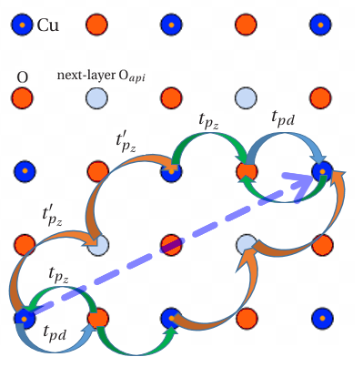
Figure 12: (Color online) Illustration of non-negligible inter-layer hopping processes contributing to $t^{\prime\prime\prime}\sim t_{pd}t_{p_{z}}t_{p_{z}}^{\prime 2}t_{p_{z}}t_{pd}/\Delta_{pd}^{2}\Delta_{z}^{3}$ and indicated by dashed arrow. Orange circles denote the in-plane oxygens, blue circles denote the copper sites above which the apical oxygens are located (orange dots), whereas shaded blue circles denote the apical oxygens located below the next-layer copper sites.

$\mathcal{\hat{H}}_{\rm eff}^{(6)}$ contains non-negligible hopping processes which are contributing to $t^{\prime\prime\prime}\sim t_{pd}^{2}t_{p_{z}}^{2}t_{p_{z}}^{\prime 2}/\Delta_{pd}^{2}\Delta_{z}^{3}$ and are originated from the inter-layer coupling (see Fig. 12). Besides, inter-plane hopping integrals are naturally enhanced by increasing $t_{p_{z}}$. As seen in Eq. (40), inter-plane hopping processes $\sim t_{pd}^{2}t_{p_{z}}^{2}t_{p_{z}}^{\prime}/\Delta_{pd}^{2}\Delta_{z}^{2}$ are leading orders for $\theta$ and $\theta^{\prime\prime}$ with opposite sign as numerically observed in Table 4.3.

Figure 13: (Color online) (a) Dispersion of the conduction band along path 1 (solid lines) and path 2 (dashed lines) with $t_{p_{z}}^{\prime}$ varied around its optimal value. (b) $\Delta E_{z}({\bf k}_{\parallel})$ with $t_{p_{z}}^{\prime}$ varied around its optimal value. The other used tight-binding parameters are given in Table 4.

X[6c]X[5c]X[5c]X[5c]X[5c]X[5c]X[5c]X[5c]X[5c]Dependence of the main in-plane and inter-plane effective hopping amplitudes on $t_{p_{z}}^{\prime}$ expressed in units of its optimal value. The other used tight-binding parameters are given in Table 4.$t_{p_{z}}^{\prime}/t_{p_{z},opt}^{\prime}$ & $t/t_{pd}$ $t^{\prime}/t$ $t^{\prime\prime}/t$ $t^{\prime\prime\prime}/t$ $t^{(4)}/t$ $\theta/t$ $\theta^{\prime}/t$ $\theta^{\prime\prime}/t$
0 0.287 -0.136 0.067 0.053 -0.026 0.0026 -0.0007 -0.0019
0.5 0.286 -0.136 0.067 0.055 -0.024 0.0141 -0.0039 -0.0115
1 0.283 -0.136 0.068 0.061 -0.017 0.0285 -0.0069 -0.0224
1.5 0.277 -0.143 0.068 0.072 -0.0007 0.0508 -0.0094 -0.0364

Concerning the hopping integral $t_{p_{z}}^{\prime}$ accounting for the coupling between inter-layer apical oxygens, Fig. 13 shows how it modifies the dispersion of the conduction band. In agreement with Eq. (27), $t_{p_{z}}^{\prime}$ does not affect the dispersion along X-M-$\Gamma$ as expected from perturbation theory Eq. (37). When $t_{p_{z}}^{\prime}$ = 0, there is naturally no inter-plane coupling and the result is similar to the case $t_{p_{z}}$ = 0. When $t_{p_{z}}^{\prime}$ is increased, the splitting between $k_{z}$ = 0 and $k_{z}=2\pi/c$ emerges along $\Gamma$-X and crosses the optimal value. Table 4.3 shows that in-plane hopping parameters are essentially independent of $t_{p_{z}}^{\prime}$, yet with the exception of $t^{\prime\prime\prime}/t$ (due to sixth order inter-layer hopping processes Eq. (55) illustrated in Fig. 12). Similarly to the previously examined $t_{p_{z}}$ case, $t_{p_{z}}^{\prime}$ yields hopping processes which essentially affect the diagonal inter-plane hopping integrals $\theta$ and $\theta^{\prime\prime}$, with opposite sign as numerically observed in Table 4.3.

Figure 14: (Color online) The exact dispersion of the conduction band along path 1and path 2 (red full lines) is compared to the effective one-band dispersion. i) With all hopping amplitudes retained (blue dashed lines), and ii) with $t$, $t^{\prime}$, $t^{\prime\prime}$, $t^{\prime\prime\prime}$, $\theta$, and $\theta^{\prime\prime}$ retained, only (green dotted lines). The used tight-binding parameters are given in Table 4, together with $t/t_{pd}=0.283$.

4.4 Numerical approach: optimal parameters

Having clarified the role of all tight-binding parameters entering Eq. (15) we now set them to their optimal value. After diagonalizing the Hamiltonian matrix Eq. (17), we apply the Fourier transform of the Cu:3d${}_{x^{2}-y^{2}}$ band and we obtain the numerical value of the microscopic hopping parameters which ultimately parameterize the conduction band through the one-band effective dispersion Eqs. (30) and (31). In-plane hopping parameters are given by: $t^{\prime}/t=-0.1364$, $t^{\prime\prime}/t=0.0677$, $t^{\prime\prime\prime}/t=0.0608$, $t^{(4)}/t=-0.0166$, $t^{(5)}/t=-0.0017$, $t^{(6)}/t=0.0125$, $t^{(7)}/t=0.0071$. Inter-plane hopping parameters are given by: $\theta/t=0.0285$, $\theta^{\prime}/t=-0.0070$, $\theta^{\prime\prime}/t=-0.0224$, $\theta^{\prime\prime\prime}/t=0.0068$, $\theta^{(4)}/t=-0.0052$, $\theta^{(5)}/t=-0.0047$ and t${}_{\left(0,0,c\right)}/t=-0.0007$. Fig. 14 shows the almost perfect fit of the one-band effective dispersion of the conduction band Eq. (29). Simplifying the effective model by retaining the largest in-plane ($t^{\prime}/t$, $t^{\prime\prime}/t$, and $t^{\prime\prime\prime}/t$) and out-of-plane ($\theta/t$, and $\theta^{\prime\prime}/t$) hopping integrals yields a good fit, too, yet with a small discrepancy along $\Gamma$-X. This approximation should nevertheless be sufficient for further purposes.

4.5 Fermi surface and density of states

Let us now turn to the Fermi surfaces following from our model. In Fig. 15 we plot projections of the 3D Fermi surface onto the ${\bf k}_{\parallel}$-plane for three important density values: half-filling (n = 1), an underdoped case (n = 0.875) and an overdoped one (n = 0.78). These projections are plotted for several positive values of $k_{z}$ as they depend on —$k_{z}$—, only. At half-filling (Fig. 15(a)), we obtain hole-like, cylindrical Fermi surfaces, for all values of $k_{z}$. They are open in $k_{z}$-direction and closed in the ${\bf k}_{\parallel}$ plane. In fact, in this case, $k_{z}$ has very little influence on the projected Fermi surface (PFS) in general, and virtually none for ${\bf k}_{\parallel}$ along $\Gamma$-M since in that case, E(${\bf k}$) very weakly depends on $k_{z}$. We further notice that the hopping amplitudes beyond $t$ no longer lead to a nested Fermi surface.

Figure 15: (Color online) Projection of the Fermi surfaces on the basal plane for several representative values of $k_{z}$ and electron density. (a) n = 1.0 (half-filling), (b) n = 0.875 (underdoped), and (c) n = 0.78 (overdoped). Parameter: $k_{z}=0$ (black full line), $k_{z}=\pi/2c$ (green dashed line), $k_{z}=\pi/c$ (green dotted line), $k_{z}=3\pi/2c$ (green full line), and $k_{z}=2\pi/c$ (black dashed line). The used tight-binding parameters are given in Table 4.

In the 1/8 hole doped case, Fig. 15(b), the Fermi surface retains its closed cylindrical shape. Astonishingly enough, the PFS around $\Gamma$ (Z’) for $k_{z}=2\pi/c$ (0) are nested, with a nesting vector ${\bf Q}\simeq(0.84,0.84)\pi/a$. One might then infer that our model is most prone to develop an incommensurate magnetic instability in this case, which might result in the formation of a stripe order (a combination of charge-density-wave and spin-density-wave modulations) that has been reported in Eu-LSCO [82], Nd-LSCO [29, 83] and LBCO [84, 83]. Besides, the influence of $k_{z}$ on the PFSs is stronger than at half-filling. Indeed, for $k_{z}=0$, the PFSs splits into two closed pieces: a smaller nested one centered around the Z’-point and a larger one centered around the $\Gamma$-point that even goes beyond the X and Y points of the square lattice. This piece has both hole and electron characters, depending on whether ${\bf k}_{\parallel}$ is rather on the nodal directions, or not. For $k_{z}=2\pi/c$ the roles of $\Gamma$ and Z’ are exchanged. For $k_{z}$ close to $\pi/c$, the two pieces join and the PFS shows hole-like character, only. Let us stress that the PFS for $k_{z}=0$ is in good agreement with 2D Fermi surface map experimentally obtained via ARPES [80, 81] and in LDA for hole doped LSCO cuprate [47, 51].

The PFSs consist of two pieces for all values of $k_{z}$. For small values of $k_{z}$ a smaller electron-like piece is centered around Z’, while the larger one is centered around the $\Gamma$-point. Again, this piece has both hole and electron character, depending on the direction of ${\bf k}_{\parallel}$. For large values of $k_{z}$ the roles of $\Gamma$ and Z’ are again exchanged. In fact, such split PFSs, together with the staggering of their size and straight and rounded shapes have been recently observed in ARPES experiment on overdoped ($\delta=22\%$) LSCO [41]. Since these features may neither be accounted for on the square lattice nor on the cubic one, they originate from the BCT structure. Furthermore it gives rise to peculiar large momentum-low energy excitations that are absent in simpler models.

Truly, these PFSs may equally well be obtained using the conduction band arising from the diagonalization of the Hamiltonian Eq. (17) or with its tight-binding form Eqs. (30) and (31), in a broad density range around half-filling. Given the rather involved form of the full tight-binding model it is tempting to neglected the smallest hopping amplitudes. This leads to retain nearest neighbor hopping amplitudes, $t$ and $\theta$, followed by $t^{\prime}$, $t^{\prime\prime}$, $t^{\prime\prime\prime}$, $\theta^{\prime}$, $\theta^{\prime\prime}$, and $\theta^{\prime\prime\prime}$, only (see Table 4.2 and Table 4.2). This approximation suffices to reproduce the Fermi surfaces with a high accuracy in all considered cases. One may then further consider neglecting $\theta^{\prime}$ and $\theta^{\prime\prime\prime}$ as well, since the so obtained conduction band is in very good agreement with the exact one (see Fig. 14). At half-filling, the resulting PFSs are in excellent agreement with the exact ones. Yet, already from $\delta=1/8$ on, the agreement degrades and, e. g., the (in-plane) PFSs no longer close around $\Gamma$ and $Z^{\prime}$, but around $M$. Yet, it only takes a small increase in doping to recover this feature. Finally, further simplifications such as neglecting $\theta^{\prime\prime}$ as well, result into an even poorer account of the conduction band. This may hardly come as a surprise given the above discussed slow convergence of the perturbative calculation of the effective model, which itself follows from the relatively small value of the charge transfer gap, and which unavoidably generates a larger number of non-negligible hopping amplitudes.

Figure 16: (Color online) The density of states of: our effective 3D model Eq. (29) (blue dashed-dotted line), the corresponding 2D model (black solid line), the tight-binding model to nearest neighbor only on the square (dotted red line) and cubic (green dashed line) lattices. Right inset: the Van Hove singularity of our model close to the bottom of the band. Left inset: the plateau exhibited by our model and surrounded by two Van Hove singularities in the vicinity of the middle of the band.

The density of states of our model is shown in Fig. 16, where it is compared to the simpler model where inter-plane hopping is set to zero. Comparison to nearest neighbor only hopping on both the square and the cubic lattices is performed, too. Interestingly, our three-dimensional model inherits features from both cases. Indeed, the density of states at the bottom of the band and at the top of the band is finite, as in the 2D case. Yet, it now exhibits a plateau surrounded by two Van Hove singularities in the vicinity of the middle of the band as for the cubic lattice. However, the plateau centered around $-0.6t$ is of considerably narrower width, as a consequence of the anisotropy of the model. Expressed in terms of the charge carrier density, the plateau extends from (1-$\delta$) = 0.81 to (1-$\delta$) = 0.89. Furthermore, one notices an additional Van Hove singularity for small density; it does not exhibit any counterpart for large density, as is expected for a particle-hole symmetric model. Finally, the 3D case remains strikingly close to the 2D one. This behavior finds its explanation when expanding Eq. (30) around the bottom of the band that is located at the $\Gamma$-point. One finds $E_{cb}({\bf k})=\epsilon_{0}+\epsilon_{1}(k_{x}^{2}+k_{y}^{2})$ where the $k_{z}$-dependence is missing. A similar behavior is found in the vicinity of the top of the band. The lack of $k_{z}$-dependence above the symmetry lines X-M-$\Gamma$ contributes to this feature, too.

5 Summary and conclusion

Summarizing, we have re-analyzed the conduction band relevant to single-layer La-based superconducting cuprates in the tight-binding framework. We have shown that it naturally emerges from an eight-band model involving two copper orbitals and six oxygen orbitals. As a consequence of their strong mutual hybridization, longer-ranged tight-binding parameters were taken into account. In particular, we obtained that the retained apical oxygen orbitals are not only crucial to the dispersion of the band perpendicular to the basal plane, but also significantly renormalize the in-plane dispersion as compared to the Emery model. This allowed us to accurately reproduce the DFT results of Markiewicz et al.[47], as well as to shed light on the peculiar $k_{z}$-dependence of the conduction band.

We then proceeded to the determination of the parameters entering the tight-binding Hamiltonian characterizing the conduction band. We first applied the Rayleigh-Schrödinger perturbation theory in order to unravel the microscopic processes contained in the eight-band model that determine the various hopping parameters entering the effective low-energy model. We have shown that the model extends the Emery model on two aspects since, on one hand, accounting for apical oxygens significantly affects the in-plane hopping amplitudes (see Table 4.2), and, on the other hand, it gives birth to out-of-plane dispersion. It turns out that perturbation theory to fifth order is mandatory to obtain non-vanishing layer to layer hopping that we found to be primarily governed by apical oxygen orbitals. This extends the 3D model proposed by Markiewicz et al.[47] (see Eq. (37)). Yet, because of the relatively small value of the charge transfer gap, the perturbative approach lacks accuracy.

We then overcame this difficulty by directly computing the hopping parameters through the Fourier transform of the numerically obtained conduction band Eq. (43). This leads to longer ranged hopping amplitudes that slowly decay with distance, and one needs to take many of them into account in order to accurately reproduce the conduction band and the Fermi surfaces. As revealed by Table 4.2 the so obtained main in-plane hopping amplitudes are in very good agreement with the ones used to fit the Fermi surfaces obtained with ARPES experiments on La-based cuprates [80, 81]. In particular, we found $t^{\prime}/t\simeq-0.1$ and $t^{\prime\prime}/t^{\prime}\simeq-0.5$ and we obtained, in addition, $(|t^{\prime}|+|t^{\prime\prime}|)/t\simeq 0.2$ as reported for overdoped La_1.78Sr_0.22CuO₄[80, 81, 85]. Furthermore, we found $t^{\prime\prime\prime}\simeq t^{\prime\prime}$, which was empirically used to model ARPES data or DFT calculations [47, 74]. Regarding inter-layer couplings (see Table 4.2), we found the magnitude of $\theta^{\prime}$ to be smaller than the one of $\theta$ and $\theta^{\prime\prime}$. Furthermore, the relation between $\theta$, $\theta^{\prime}$, $\theta^{\prime\prime}$, and $\theta^{\prime\prime\prime}$ assumed in Eq. (6)[47] could not be recovered, so that the leading contribution to the dispersion perpendicular to the layers is indeed given by Eq. (37). In the doped case our model yields peculiar Fermi surfaces which projections on the basal plane alternate in size and shape. Since this may not arise in tight-binding models on square or cubic lattices this may be seen as a signature of the body-centered tetragonal structure that is at the heart of this work. It is compatible with recent ARPES measurements of the 3D Fermi surface of overdoped LSCO [41]. Finally, it would be of interest to carry out the corresponding analysis to other cuprate families, or to highly anisotropic oxides such as PdCoO₂ [86, 87], which structure entails shifted layers such as Bi-2212 [47] or Tl-2201 [88, 89]. We also unraveled that simplifying Eqs. (30) and (31) down to a model that only entails the in-plane $t$, $t^{\prime}$, $t^{\prime\prime}$, and $t^{\prime\prime\prime}$ as well as the out-of-plane $\theta$, and $\theta^{\prime\prime}$ hopping amplitudes (given in Tables 4.2 and 4.2) yields a reasonable description of the conduction band and should therefore suffice for future purposes. For instance, it would be of interest to understand how the found peculiar form of nesting and interaction generate magnetic or pairing instabilities within a Hubbard model on the BCT lattice. Work along this line is in progress.

Acknowledgments.  The authors acknowledge the financial support of the Ministère de la Recherche, the Région Normandie and the French Agence Nationale de la Recherche (ANR), through the program Investissements d’Avenir (ANR-10-LABX-09-01) and LabEx EMC3. The authors gratefully acknowledge G. A. Sawatsky, A. F. Santander-Syro, A. M. Oleś, V. H. Dao and O. Juillet for inspiring discussions.

Appendix A Lindgren’s formulation of Rayleigh-Schrödinger perturbation theory

The above Eqs. (33, 34, 35, 36) have been derived using the Rayleigh-Schrödinger perturbation theory. More specifically, we made use of Lindgren’s formulation [90] to set up an effective tight-binding Hamiltonian and to put forward the microscopic origin of the various hopping amplitudes. Below, we summarize the main steps leading to an effective Hamiltonian at a given order in perturbation theory. The Hamiltonian $\hat{H}$ Eqs. (16, 17) is separated into its diagonal part that plays the role of the unperturbed Hamiltonian, $\sum_{{\bf k},\sigma}\mathcal{\hat{H}}_{0,\sigma}({\bf k})\equiv\sum_{{\bf k},\sigma}\sum_{\nu}\epsilon_{\nu}({\bf k})\hat{\Psi}_{{\bf k},\sigma,\nu}^{\dagger}\hat{\Psi}_{{\bf k},\sigma,\nu}^{\phantom{\dagger}}$, and its off-diagonal part this is considered as the perturbation $\sum_{{\bf k},\sigma}\mathcal{\hat{H}}_{1,\sigma}({\bf k})$

$$\mathcal{\hat{H}}=\sum_{{\bf k},\sigma}\left(\mathcal{\hat{H}}_{0,\sigma}({\bf k})+\mathcal{\hat{H}}_{1,\sigma}({\bf k})\right)\>.$$ (44)

Usually, perturbation theory is applied to problems lacking an exact solution. In our case the latter has been found, but in numerical form, only, and our goal is not to recover it. Instead, it is to shed light on both how the perturbation generates the dispersion of the conduction band, and on the microscopical origin of the various hopping amplitudes entering the effective one-band model. In Lindgren’s approach [90], the effective Hamiltonian acting on the low energy sector of the Hilbert space, here spanned by $|d_{{\bf k},\sigma}\rangle$, is expressed in terms of a wave operator $\hat{\Omega}({\bf k})$ [91] as:

$$\begin{split}\mathcal{\hat{H}}_{\rm eff}^{(i)}=\sum_{{\bf k}}|d_{\bf k}\rangle\langle d_{\bf k}|\mathcal{\hat{H}}_{1}({\bf k})\left(\hat{\Omega}^{(0)}({\bf k})+\hat{\Omega}^{(1)}({\bf k})+\hat{\Omega}^{(2)}({\bf k})+...\right.\\ +\left.\hat{\Omega}^{(i-1)}({\bf k})\right)\>\>,\end{split}$$ (45)

where the dull index $\sigma$ is omitted for simplicity. Having measured all energies relative to $\epsilon_{d}$ forces the zeroth order contribution to vanish. To zeroth order the wave operator is simply the projection operator onto the low-energy sector of our model:

$$\hat{\Omega}^{(0)}({\bf k})=|d_{\bf k}\rangle\langle d_{\bf k}|\>.$$ (46)

Starting from Schrödinger’s equation, Lindgren obtained a recursion formula for $\hat{\Omega}^{(l)}({\bf k})$:

$$= (1-|d_{\bf k}\rangle\langle d_{\bf k}|)\mathcal{\hat{H}}_{1}({\bf k})\hat{\Omega}^{(l-1)}({\bf k})$$ (47)

$$-\sum_{m=1}^{l-1}\hat{\Omega}^{(l-m)}({\bf k})\mathcal{\hat{H}}_{1}({\bf k})\hat{\Omega}^{(m-1)}({\bf k})\>.$$

The lowest orders are then explicitly obtained as:

$$\hat{\Omega}^{(1)}({\bf k})=\sum_{\nu}|\nu_{\bf k}\rangle\langle d_{\bf k}|\frac{\langle\nu_{\bf k}|\mathcal{\hat{H}}_{1}({\bf k})|d_{\bf k}\rangle}{\epsilon_{d}-\epsilon_{\nu}({\bf k})}$$ (48)

$$\hat{\Omega}^{(2)}({\bf k})=\sum_{\nu}|\nu_{\bf k}\rangle\langle d_{\bf k}|\frac{\langle\nu_{\bf k}|\mathcal{\hat{H}}_{1}({\bf k})\hat{\Omega}^{(1)}({\bf k})-\hat{\Omega}^{(1)}({\bf k})\mathcal{\hat{H}}_{1}({\bf k})|d_{\bf k}\rangle}{\epsilon_{d}-\epsilon_{\nu}({\bf k})}$$ (49)

$$\hat{\Omega}^{(3)}({\bf k})=\sum_{\nu}|\nu_{\bf k}\rangle\langle d_{\bf k}|\times$$ (50)

$$\frac{\langle\nu_{\bf k}|\mathcal{\hat{H}}_{1}({\bf k})\hat{\Omega}^{(2)}({\bf k})\!-\!\hat{\Omega}^{(1)}({\bf k})\mathcal{\hat{H}}_{1}({\bf k})\hat{\Omega}^{(1)}({\bf k})\!-\!\hat{\Omega}^{(2)}({\bf k})\mathcal{\hat{H}}_{1}({\bf k})|d_{\bf k}\rangle}{\epsilon_{d}-\epsilon_{\nu}({\bf k})}$$

$$\hat{\Omega}^{(4)}({\bf k})=\sum_{\nu}|\nu_{\bf k}\rangle\langle d_{\bf k}|$$ (51)

$$\times\frac{\langle\nu_{\bf k}|\left[\mathcal{\hat{H}}_{1}({\bf k})\hat{\Omega}^{(3)}({\bf k})-\hat{\Omega}^{(1)}({\bf k})\mathcal{\hat{H}}_{1}({\bf k})\hat{\Omega}^{(2)}({\bf k})\right.}{\epsilon_{d}-\epsilon_{\nu}({\bf k})}$$

$$-\frac{\left.\hat{\Omega}^{(2)}({\bf k})\mathcal{\hat{H}}_{1}({\bf k})\hat{\Omega}^{(1)}({\bf k})+\hat{\Omega}^{(3)}({\bf k})\mathcal{\hat{H}}_{1}({\bf k})\right]|d_{\bf k}\rangle}{\epsilon_{d}-\epsilon_{\nu}({\bf k})}\,,$$

where we have kept (the here vanishing) $\epsilon_{d}$, for clarity. Hence

$$\mathcal{\hat{H}}_{\rm eff}^{(4)} =\sum_{{\bf k}}|d_{\bf k}\rangle\langle d_{\bf k}|\left[\epsilon_{d}+\sum_{\nu}\frac{|h_{\nu}({\bf k})|^{2}}{\epsilon_{d}-\epsilon_{\nu}({\bf k})}\right.$$ (52)

$$+\sum_{\nu,\nu^{\prime}}\frac{h_{\nu}({\bf k})g_{\nu,\nu^{\prime}}({\bf k})h_{\nu^{\prime}}({\bf k})}{(\epsilon_{d}-\epsilon_{\nu}({\bf k}))(\epsilon_{d}-\epsilon_{\nu^{\prime}}({\bf k}))}$$

$$+\sum_{\nu,\nu^{\prime},\nu^{\prime\prime}}\frac{h_{\nu}({\bf k})g_{\nu,\nu^{\prime}}({\bf k})g_{\nu^{\prime},\nu^{\prime\prime}}({\bf k})h_{\nu^{\prime\prime}}^{*}({\bf k})}{(\epsilon_{d}-\epsilon_{\nu}({\bf k}))(\epsilon_{d}-\epsilon_{\nu^{\prime}}({\bf k}))(\epsilon_{d}-\epsilon_{\nu^{\prime\prime}}({\bf k}))}$$

$$-\left.\sum_{\nu,\nu^{\prime}}\frac{|h_{\nu}({\bf k})|^{2}|h_{\nu^{\prime}}({\bf k})|^{2}}{(\epsilon_{d}-\epsilon_{\nu^{\prime}}({\bf k}))^{2}(\epsilon_{d}-\epsilon_{\nu^{\prime}}({\bf k}))}\right]\,,$$

with

$$\mathcal{\hat{H}}_{1,d,\nu} =\sum_{{\bf k}}t_{pd}\left(h_{3}({\bf k})|d_{\bf k}\rangle\langle p_{x,{\bf k}}^{(X)}|+h_{4}({\bf k})|d_{\bf k}\rangle\langle p_{y,{\bf k}}^{(Y)}|\right)$$ (53)

$$\mathcal{\hat{H}}_{1,\nu,\nu^{\prime}} =\sum_{{\bf k}}\sum_{\nu,\nu^{\prime}}g_{\nu,\nu^{\prime}}({\bf k})|\nu_{\bf k}\rangle\langle\nu_{\bf k}^{\prime}|\>,$$

where $h_{3}({\bf k})=2it_{pd}p_{x}$ and $h_{4}({\bf k})=-2it_{pd}p_{y}$. The matrix elements $\langle\nu_{\bf k}|\mathcal{\hat{H}}_{1}({\bf k})|\nu^{\prime}_{\bf k}\rangle$ are denoted by $g_{\nu,\nu^{\prime}}({\bf k})$. Regarding the inter-layer coupling given by Eq. (27), it turns out to appear at fifth order, from the contributions to $\mathcal{\hat{H}}_{\rm eff}^{(5)}$ reading:

$$\sum_{\nu,\nu^{\prime},\nu^{\prime\prime},\nu^{\prime\prime\prime}}\frac{h_{\nu}({\bf k})g_{\nu,\nu^{\prime}}({\bf k})g_{\nu^{\prime},\nu^{\prime\prime}}({\bf k})g_{\nu^{\prime\prime},\nu^{\prime\prime\prime}}({\bf k})h_{\nu^{\prime\prime\prime}}^{*}({\bf k})}{(\epsilon_{d}-\epsilon_{\nu}({\bf k}))(\epsilon_{d}-\epsilon_{\nu^{\prime}}({\bf k}))(\epsilon_{d}-\epsilon_{\nu^{\prime\prime}}({\bf k}))(\epsilon_{d}-\epsilon_{\nu^{\prime\prime\prime}}({\bf k}))}\>.$$ (54)

Besides, inter-layer couplings may significantly contribute to in-plane hopping amplitudes. This is especially relevant to $t^{\prime\prime\prime}$, from contribution to $\mathcal{\hat{H}}_{\rm eff}^{(6)}$ of the form:

$$\sum_{\nu,\nu^{\prime},\nu^{\prime\prime}} \frac{h_{\nu}({\bf k})g_{\nu,\nu^{\prime}}({\bf k})g_{\nu^{\prime},\nu^{\prime\prime}}({\bf k})}{(\epsilon_{d}-\epsilon_{\nu}({\bf k}))(\epsilon_{d}-\epsilon_{\nu^{\prime}}({\bf k}))(\epsilon_{d}-\epsilon_{\nu^{\prime\prime}}({\bf k}))}$$ (55)

$$\times\sum_{\nu^{\prime\prime\prime},\nu^{\prime\prime\prime\prime}} \frac{g_{\nu^{\prime\prime},\nu^{\prime\prime\prime}}({\bf k})g_{\nu^{\prime\prime\prime},\nu^{\prime\prime\prime\prime}}({\bf k})h_{\nu^{\prime\prime\prime\prime}}^{*}({\bf k})}{(\epsilon_{d}-\epsilon_{\nu^{\prime\prime\prime}}({\bf k}))(\epsilon_{d}-\epsilon_{\nu^{\prime\prime\prime\prime}}({\bf k}))}\,.$$

References

• [1] K. A. Müller, J. G. Bednorz, Z. Phys. B: Condens. Matter 1986, 64, 189.
• [2] E. Dagotto, Rev. Mod. Phys. 1994, 66, 763.
• [3] P. A. Lee, N. Nagaosa, X.-G. Wen, Rev. Mod. Phys. 2006, 78, 17.
• [4] E. Fradkin, S. A. Kivelson, Nat. Phys. 2012, 8, 864.
• [5] B. Keimer, S. A. Kivelson, M. R. Norman, S. Uchida, J. Zaanen, Nature 2015, 518, 179.
• [6] C. Proust, L. Taillefer, Annu. Rev. Condens. Matter Phys. 2019, 10, 409.
• [7] R. von Helmolt, J. Wecker, B. Holzapfel, L. Schultz, K. Samwer, Phys. Rev. Lett. 1993, 71, 2331.
• [8] Y. Tomioka, A. Asamitsu, Y. Moritomo, H. Kuwahara, Y. Tokura, Phys. Rev. Lett. 1995, 74, 5108.
• [9] B. Raveau, A. Maignan, V. Caignaert, J. Solid State Chem. 1995, 117, 424.
• [10] A. Maignan, Ch. Simon, V. Caignaert, B. Raveau, Solid State Commun. 1995, 96, 623.
• [11] H. Kawazoe, M. Yasukawa, H. Hyodo, M. Kurita, H. Yanagi, H. Hosono, Nature 1997, 389, 939.
• [12] T. Harada, K. Fujiwara, A. Tsukazaki, APL Materials 2018, 6, 046107.
• [13] I. Terasaki, Y. Sasago, K. Uchinokura, Phys. Rev. B 1997, 56, R12685.
• [14] A. C. Masset, C. Michel, A. Maignan, M. Hervieu, O. Toulemonde, F. Studer, B. Raveau, J. Hejtmanek, Phys. Rev. B 2000, 62, 166.
• [15] I. Matsubara, R. Funahashi, T. Takeuchi, S. Sodeoka, T. Shimizu, K. Ueno, Appl. Phys. Lett. 2001, 78, 3627.
• [16] M. Miclau, J. Hejtmanek, R. Retoux, K. Knizek, Z. Jirak, R. Frésard, A. Maignan, S. Hébert, M. Hervieu, C. Martin, Chem. Mater. 2007, 19, 4243.
• [17] H. Ohta, S. Kim, Y. Mune, T. Mizoguchi, K. Nomura, S. Ohta, T. Nomura, Y. Nakanishi, Y. Ikuhara, M. Hirano, H. Hosono, K. Koumoto, Nat. Mater. 2007, 6, 129.
• [18] N. Wang, H. J. Chen, H. C. He, W. Norimatsu, M. Kusunoki, K. Koumoto, Sci. Rep. 2013, 3, 3449.
• [19] E. Guilmeau, M. Poienar, S. Kremer, S. Marinel, S, Hébert, R. Frésard, A. Maignan, Solid State Commun. 2011, 151, 1798.
• [20] N. Reyren, S. Thiel, A. D. Caviglia, L. F. Kourkoutis, G. Hammerl, C. Richter, C. W. Schneider, T. Kopp, A.-S. Rüetschi, D. Jaccard, M. Gabay, D. A. Muller, J.-M. Triscone, J. Mannhart, Science 2007, 317, 1196.
• [21] D. B. McWhan, A. Menth, J. P. Remeika, W. F. Brinkman, T. M. Rice, Phys. Rev. B 1973, 7, 1920.
• [22] K. Held, G. Keller, V. Eyert, D. Vollhardt, V. I. Anisimov, Phys. Rev. Lett. 2001, 86, 5345.
• [23] P. Limelette, A. Georges, D. Jérome, P. Wzietek, P. Metcalf, J. M. Honig, Science 2003, 302, 89.
• [24] C. Grygiel, Ch. Simon, B. Mercey, W. Prellier, R. Frésard, P. Limelette, Appl. Phys. Lett. 2007, 91, 262103.
• [25] P. W. Anderson, Science 1987, 235, 1196.
• [26] A. M. S. Tremblay, B. Kyung, D. Sénéchal, J. Low Temp. Phys. 2006, 32, 424.
• [27] A. Leprévost, O. Juillet, R. Frésard, New J. Phys. 2015, 17, 103023.
• [28] B.-X. Zheng, C.-M. Chung, P. Corboz, G. Ehlers, M.-P. Qin, R. M. Noack, S. R. White, S. Zhang, G. K.-L. Chan, Science 2017, 358, 1155.
• [29] J. Tranquada, B. Sternlieb, J. Axe, Y. Nakamura, S. Uchida. Nature 1995, 375, 561; J. M. Tranquada, J. D. Axe, N. Ichikawa, A. R. Moodenbaugh, Y. Nakamura, S. Uchida, Phys. Rev. Lett. 1997, 78, 338.
• [30] M. Raczkowski, R. Frésard, A. M. Oleś, Europhys. Lett. 2006, 76, 128.
• [31] J. P. F. LeBlanc, A. E. Antipov, F. Becca, I. W. Bulik, G. K.-L. Chan, C.-M. Chung, Y. Deng, M. Ferrero, T. M. Henderson, C. A. Jimnez-Hoyos, E. Kozik, X.-W. Liu, A. J. Millis, N. V. Prokofev, M. Qin, G. E. Scuseria, H. Shi, B. V. Svistunov, L. F. Tocchio, I. S. Tupitsyn, S. R. White, S. Zhang, B.-X. Zheng, Z. Zhu, E. Gull, Phys. Rev. X ${\bf 2015}$, 5, 041041.
• [32] M. Raczkowski, R. Frésard, A. M. Oleś, Phys. Rev. B 2006, 73, 174525.
• [33] K. Ido, T. Ohgoe, M. Imada, Phys. Rev. B 2018, 97, 045138.
• [34] E. W. Huang, C. B. Mendl, H.-C. Jiang, B. Moritz, T. P. Devereaux, npj Quantum Materials 2018, 3, 22.
• [35] E. Pavarini, I. Dasgupta, T. Saha-Dasgupta, O. Jepsen, O. K. Andersen, Phys. Rev. Lett. 2001, 87, 047003.
• [36] P. G. Radaelli, D. G. Hinks, A. W. Mitchell, B. A. Hunter, J. L. Wagner, B. Dabrowski, K. G. Vandervoort, H. K. Viswanathan, J. D. Jorgensen, Phys. Rev. B 1994, 49, 4163.
• [37] J. P. Locquet, J. Perret, J. Fompeyrine, E. Mächler, J. W. Seo, G. Van Tendeloo, Nature 1998, 394, 453.
• [38] H. Sato, A. Tsukada, M. Naito, A. Matsuda, Phys. Rev. B 2000, 61, 12447.
• [39] P. Corboz, T. M. Rice, M. Troyer, Phys. Rev. Lett. 2014, 113, 046402.
• [40] T. Misawa, M. Imada, Phys. Rev. B 2014, 90, 115137.
• [41] M. Horio, K. Hauser, Y. Sassa, Z. Mingazheva, D. Sutter, K. Kramer, A. Cook, E. Nocerino, O. K. Forslund, O. Tjernberg, M. Kobayashi, A. Chikina, N. B. M. Schröter, J. A. Krieger, T. Schmitt, V. N. Strocov, S. Pyon, T. Takayama, H. Takagi, O. J. Lipscombe, S. M. Hayden, M. Ishikado, H. Eisaki, T. Neupert, M. Månsson, C. E. Matt, J. Chang, Phys. Rev. Lett. 2018, 121, 077004.
• [42] N. Nguyen, J. Choisnet, M. Hervieu, B. Raveau, J. Solid State Chem. 1981, 39, 120; N. Nguyen, F. Studer, B. Raveau, J. Phys. Chem. Solids 1983, 44, 389.
• [43] O. K. Andersen, A. I. Liechtenstein, O. Jepsen, F. Paulsen, J. Phys. Chem. Solids 1995, 56, 1573; O. K. Andersen, S. Y. Savrasov, O. Jepsen, A. I. Liechtenstein, J. Low Temp. Phys. 1996, 105, 285.
• [44] T. M. Mishonov, J. O Indekeu, E. S. Penev, J. Phys.: Condens. Matter 2003, 15, 4429.
• [45] M. Stoev, T. M. Mishonov, Eur. Phys. J. B 2010, 73, 109.
• [46] A. Bansil, M. Lindroos, S. Sahrakorpi, R. S. Markiewicz, New J. Phys. 2005, 7, 140.
• [47] R. S. Markiewicz, S. Sahrakorpi, M. Lindroos, H. Lin, A. Bansil, Phys. Rev. B 2005, 72, 054519.
• [48] V. J. Emery, Phys. Rev. Lett. 1987, 58, 2794; V. J. Emery, G. Reiter, Phys. Rev. B 1988, 38, 4547.
• [49] C. M. Varma, Solid State Commun. 1987, 62, 681.
• [50] Y. B. Gaididei, V. M. Loktev, Phys. Status Solidi 1988, 147, 307.
• [51] M. Lindroos, S. Sahrakorpi, V. Arpiainen, R. S. Markiewicz, A. Bansil, J. Phys. Chem. Sol. 2006, 67, 244.
• [52] A. K. McMahan, R. M. Martin, S. Satpathy, Phys. Rev. B 1988, 38, 6650.
• [53] F. Mila, Phys. Rev. B 1988, 38, 11358.
• [54] M. S. Hybertsen, M. Schlüter, N. E. Christensen, Phys. Rev. B 1989, 39, 9028.
• [55] A. P. Kampf, Phys. Rep. 1994, 249, 219.
• [56] G. Dopf, A. Muramatsu, W. Hanke, Phys. Rev. B 1990, 41, 9264; G. Dopf, J. Wagner, P. Dieterich, A. Muramatsu, W. Hanke, Phys. Rev. Lett. 1992, 68, 2082; G. Dopf, A. Muramatsu, W. Hanke, Phys. Rev. Lett. 1992, 68, 353.
• [57] P. R. C. Kent, T. Saha-Dasgupta, O. Jepsen, O. K. Andersen, A. Macridin, T. A. Maier, M. Jarrell, T. C. Schulthess, Phys. Rev. B 2008, 78, 035132.
• [58] S. W. Jang, T. Kotani, H. Kino, K. Kuroki, M. J. Han, Sci. Rep. 2015, 5, 12050.
• [59] J. Labbé, J. Bok, Europhys. Lett. 1987, 3, 1225.
• [60] N. E. Hussey, M. Abdel-Jawad, A. Carrington, A. P. Mackenzie, L. Balicas, Nature 2003, 425, 814.
• [61] A. Damascelli, Z.-X. Shen, Z. Hussain, Rev. Mod. Phys. 2003, 75, 473.
• [62] D. J. Scalapino, Phys. Rep. 1995, 250, 330.
• [63] C. E. Matt, D. Sutter, A. M. Cook, Y. Sassa, M. Månsson, O. Tjernberg, L. Das, M. Horio, D. Destraz, C. G. Fatuzzo, K. Hauser, M. Shi, M. Kobayashi, V. N. Strocov, T. Schmitt, P. Dudin, M. Hoesch, S. Pyon, T. Takayama, H. Takagi, O. J. Lipscombe, S. M. Hayden, T. Kurosawa, N. Momono, M. Oda, T. Neupert, J. Chang, Nat. Commun. 2018, 9, 972.
• [64] H. Sakakibara, H. Usui, K. Kuroki, R. Arita, H. Aoki, Phys. Rev. Lett. 2010, 105, 057003.
• [65] R. Raimondi, J. H. Jefferson, L. F. Feiner, Phys. Rev. B 1996, 53, 8774.
• [66] L. F. Feiner, M. Grilli, C. Di Castro, Phys. Rev. B 1992, 45, 10647.
• [67] B. Lau, M. Berciu, G. A. Sawatzky, Phys. Rev. Lett. 2011, 106, 036401.
• [68] P. Hansmann, N. Parragh, A. Toschi, G. Sangiovanni, K. Held, New J. Phys. 2014, 16, 033009.
• [69] C. Weber, K. Haule, G. Kotliar, Phys. Rev. B 2010, 82, 125107.
• [70] T. Xiang, J. M. Wheatley, Phys. Rev. Lett. 1996, 77, 4632.
• [71] Y. Y. Peng, G. Dellea, M. Minola, M. Conni, A. Amorese, D. Di Castro, G. M. De Luca, K. Kummer, M. Salluzzo, X. Sun, X. J. Zhou, G. Balestrino, M. Le Tacon, B. Keimer, L. Braicovich, N. B. Brookes, G. Ghiringhelli, Nat. Phys. 2017, 13, 1201.
• [72] K. P. Kramer, M. Horio, S. S. Tsirkin, Y. Sassa, K. Hauser, C. E. Matt, D. Sutter, A. Chikina, N. Schröter, J. A. Krieger, T. Schmitt, V. N. Strocov, N. Plumb, M. Shi, S. Pyon, T. Takayama, H. Takagi, T. Adachi, T. Ohgi, T. Kawamata, Y. Koike, T. Kondo, O. J. Lipscombe, S. M. Hayden, M. Ishikado, H. Eisaki, T. Neupert, J. Chang, Phys. Rev. B ${\bf 2019}$, 99, 224509.
• [73] F. C. Zhang, T. M. Rice. Phys. Rev. B 1988, 37, 3759(R).
• [74] M. R. Norman, Phys. Rev. B 2007, 75, 184514.
• [75] L. M. Mattheiss, D. R. Hamann, Phys. Rev. B 1988, 38, 5012.
• [76] G. G. N. Angilella, R. Pucci, Physica B 1999, 265, 136.
• [77] S. Chakravarty, A. Sudbø, P. W. Anderson, S. Strong, Science 1993, 261, 337.
• [78] H. Ebrahimnejad, G. A. Sawatzky, M. Berciu, Nat. Phys. 2014, 10, 951.
• [79] W. A. Harrison, Elementary Electronic Structure, World Scientific 1999.
• [80] T. Yoshida, X. J. Zhou, K. Tanaka, W. L. Yang, Z. Hussain, Z.-X. Shen, A. Fujimori, S. Sahrakorpi, M. Lindroos, R. S. Markiewicz, A. Bansil, S. Komiya, Y. Ando, H. Eisaki, T. Kakeshita, S. Uchida, Phys. Rev. B 2006, 74, 224510.
• [81] T. Yoshida, X. J. Zhou, D. H. Lu, S. Komiya, Y. Ando, H. Eisaki, T. Kakeshita, S. Uchida, Z. Hussain, Z.-X. Shen, A. Fujimori, J. Phys: Condens. Matter 2007, 19, 125209.
• [82] J. Fink, V. Soltwisch, J. Geck, E. Schierle, E. Weschke, B. Büchner, Phys. Rev. B 2011, 83, 092503.
• [83] J. M. Tranquada, Physica B, 2012, 407, 1771.
• [84] M. Hücker, M. v. Zimmermann, G. D. Gu, Z. J. Xu, J. S. Wen, Guangyong Xu, H. J. Kang, A. Zheludev, J. M. Tranquada, Phys. Rev. B 2011, 83, 104506.
• [85] J. Chang, M. Månsson, S. Pailhès, T. Claesson, O. J. Lipscombe, S. M. Hayden, L. Patthey, O. Tjernberg, J. Mesot, Nat. Commun. 2013, 4, 2559.
• [86] C. W. Hicks, A. S. Gibbs, A. P. Mackenzie, H. Takatsu, Y. Maeno, E. A. Yelland, Phys. Rev. Lett. 2012, 109, 116401.
• [87] R. Daou, R. Frésard, S. Hébert, A. Maignan, Phys. Rev. B 2015, 91, 041113(R).
• [88] D. J. Singh, W. E. Pickett, Physica C 1992, 203, 193.
• [89] D. C. Peets, J. D. F. Mottershead, B. Wu, I. S. Elfimov, R. Liang, W. N. Hardy, D. A. Bonn, M. Raudsepp, N. J. C. Ingle, A. Damascelli, New J. Phys. 2007, 9, 28.
• [90] I. Lindgren, J. Phys. B 1974, 7, 2441.
• [91] C. Møller, K. Dan. Vid. Selsk. 1945, 22, 19.