Hidden symmetry and the separability of the Maxwell equation
on the Wahlquist spacetime

Abstract

We examine hidden symmetry and its relation to the separability of the Maxwell equation on the Wahlquist spacetime. After seeing that the Wahlquist spacetime is a type-D spacetime whose repeated principal null directions are shear-free and geodesic, we show that the spacetime admits three gauged conformal Killing-Yano (GCKY) tensors which are in a relation with torsional conformal Killing-Yano tensors. As a by-product, we obtain an ordinary CKY tensor. We also show that thanks to the GCKY tensors, the Maxwell equation reduces to three Debye equations, which are scalar-type equations, and two of them can be solved by separation of variables.

I Introduction

Hidden symmetry of spacetime has played an important role in the study of black hole physics. In particular, conformal Killing-Yano symmetry, known as hidden symmetry of the Kerr spacetime, has received special attention since it has been crucial to understanding the separability of various equations on a curved spacetime.

On the Kerr spacetime, the Hamilton-Jacobi equation for geodesics, the Klein-Gordon equation, and the Dirac equation can be solved by separation of variables, and these separabilities have been understood in terms of a Killing-Yano tensor. For electromagnetic and gravitational perturbations, Teukolsky Teukolsky:1972 ; Teukolsky:1973 provided the scalar-type master equations, which can be solved by separation of variables. Cohen and Kegeles Cohen:1974 showed that, if a spacetime is algebraically special and its repeated principal null direction (PND) is shear-free and geodesic, the Maxwell equation reduces to a scalar-type master equation called the Debye equation. They also showed that when their method is applied to the Kerr spacetime, the Debye equation coincides with the Teukolsky equation. Moreover, they extended their results to massless Dirac fields on algebraically special spacetimes and gravitational perturbations on vacuum spacetimes Cohen:1979 . After a while, Benn, Charlton, and Kress Benn:1997 unveiled the underlying structure of the works by Cohen and Kegeles from the viewpoint of GCKY symmetry. So far, while the GCKY symmetry has been related to obtaining the scalar-type master equations from the Dirac, Maxwell, and linearized Einstein equations, the separability of those equations has not been well understood. To fill the gap is one of the aims in this paper.

In this paper, we examine hidden symmetry of the Wahlquist spacetime Wahlquist:1968 ; Kramer:1985 ; Senovilla:1987 ; Wahlquist:1992 ; Bradley:1999 ; Mars:2001 ; Hinoue:2014 , which is a stationary, axially symmetric solution to the Einstein equation with rigidly rotating perfect fluids. According to the Goldberg-Sachs theorem, the repeated PNDs on a type-D vacuum spacetime are shear-free and geodesic. However, since the Wahlquist metric is a non-vacuum type-D spacetime, it is interesting to ask if the repeated PNDs are shear-free and geodesic. According to Cohen:1974 ; Benn:1997 , if they are so, we obtain GCKY tensors with a certain condition and hence the Maxwell equation reduces to the Debye equation. Since the Wahlquist spacetime is known to admit a torsional conformal Killing-Yano (TCKY) tensor Hinoue:2014 , there may be some relation between the gauged and torsional CKY tensors, and it is another aim of this work to clarify it. We also examine whether the Debye equation can be solved by separation of variables.

This paper is organized as follows. In the next section, we examine hidden symmetry of the Wahlquist spacetime. In Sec. III, we show that the Maxwell equation reduces to three Debye equations, and two of them can be solved by separation of variables. The last section is devoted to summary and discussion. In appendix, we briefly show the separability of the Dirac equation on the Wahlquist spacetime. We summarize our terminology for spacetimes in FIG. 2 and relations between hidden symmetry of the Wahlqusit spacetime in FIG. 2.

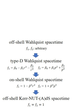
Figure 1: Our terminology for spacetimes in this work, which depend on the functions $f_{1}$ and $f_{2}$.

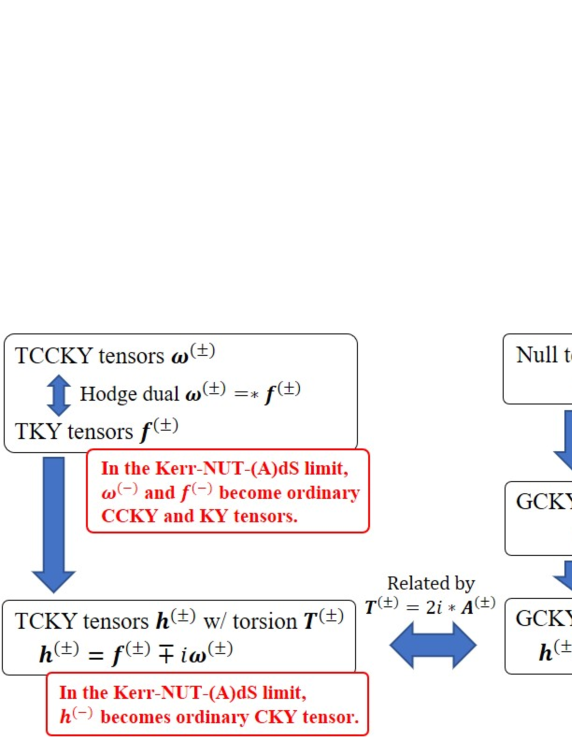
Figure 2: Relations between hidden symmetry of the Wahlquist spacetime. The arrows show that, if $A\Rightarrow B$, $B$ is induced or constructed from $A$.

II Hidden symmetry of the Wahlquist spacetime

In this section, we examine hidden symmetry of the Wahlquist spacetime. Although some results about the torsional conformal Killing-Yano tensor on this spacetime were already found in Hinoue:2014 , the aim of this section is to elucidate the gauged conformal Killing-Yano tensors and their relations to the torsional one.

II.1 Off-shell Wahlquist metric

The Wahlquist metric (see, e.g. Hinoue:2014 ) is written as

$$ds^{2}=-\frac{{\cal Q}}{r^{2}+p^{2}}(d\tau-p^{2}d\sigma)^{2}+\frac{r^{2}+p^{2}}{{\cal Q}f_{1}}dr^{2}+\frac{r^{2}+p^{2}}{{\cal P}f_{2}}dp^{2}+\frac{{\cal P}}{r^{2}+p^{2}}(d\tau+r^{2}d\sigma)^{2}\,,$$ (1)

where ${\cal Q}$ and ${\cal P}$ are given by

$${\cal Q}= Q_{0}+a_{2}r\sqrt{1-\beta^{2}r^{2}}+\nu_{0}r^{2}+\frac{\mu_{0}}{\beta^{2}}\left[r^{2}-\frac{r\,\textrm{Arcsin}(\beta r)\sqrt{1-\beta^{2}r^{2}}}{\beta}\right]\,,$$ (2)

$${\cal P}= Q_{0}+a_{1}p\sqrt{1+\beta^{2}p^{2}}-\nu_{0}p^{2}-\frac{\mu_{0}}{\beta^{2}}\left[p^{2}-\frac{p\,\textrm{Arcsin}(\beta p)\sqrt{1+\beta^{2}p^{2}}}{\beta}\right]\,,$$ (3)

and $f_{1}$ and $f_{2}$ are given by

$$f_{1}=1-\beta^{2}r^{2}\,,\qquad f_{2}=1+\beta^{2}p^{2}\,,$$ (4)

with constants $Q_{0}$, $a_{1}$, $a_{2}$, $\nu_{0}$, $\mu_{0}$ and $\beta$.

To handle a wider class of metrics including the Wahlquist metric, we consider the metric (1) with ${\cal Q}$, ${\cal P}$, $f_{1}$, and $f_{2}$ replaced with arbitrary functions of single variable, ${\cal Q}(r)$, ${\cal P}(p)$, $f_{1}(r)$, and $f_{2}(p)$ and call it the off-shell Wahlquist metric. As a special class, the Wahlquist metric with $\beta=0$ is called the Kerr-NUT-(A)dS metric. Moreover, the off-shell Wahlquist metric with $f_{1}=f_{2}=1$ is called the off-shell Kerr-NUT-(A)dS metric.

II.2 Torsional Killing-Yano tensor and Killing-Stäckel tensor

In Hinoue:2014 , it was shown that the off-shell Wahlquist metric admits torsional Killing-Yano (TKY) tensors ${\bm{f}}^{(\pm)}$ and torsional closed conformal Killing-Yano (TCCKY) tensors ${\bm{\omega}}^{(\pm)}$, defined by the equations

$$\nabla^{(T)}_{a}f_{bc} =\nabla^{(T)}_{[a}f_{bc]}\,,$$ (5)

$$\nabla^{(T)}_{a}\omega_{bc} =g_{ab}\xi^{(T)}_{c}-g_{ac}\xi^{(T)}_{b}\,,$$ (6)

where

$$\xi^{(T)}_{a}=\frac{1}{3}\nabla^{(T)b}\omega_{ba}\,.$$ (7)

Here, $\nabla^{(T)}_{a}$ is the covariant derivative with totally antisymmetric torsion ${\bm{T}}$ and it acts on a 2-form ${\bm{\Psi}}$ as

$$\nabla^{(T)}_{a}\Psi_{bc}=\nabla_{a}\Psi_{bc}+\frac{1}{2}T_{ab}{}^{d}\Psi_{cd}-\frac{1}{2}T_{ac}{}^{d}\Psi_{bd}\,.$$ (8)

To describe such symmetries, it is convenient to introduce the orthonormal basis $\{{\bm{e}}^{\mu}\}$ as

$${\bm{e}}^{0}=\sqrt{\frac{{\cal Q}}{r^{2}+p^{2}}}(d\tau-p^{2}d\sigma)\,,\quad{\bm{e}}^{1}=\sqrt{\frac{r^{2}+p^{2}}{{\cal Q}f_{1}}}dr\,,\quad{\bm{e}}^{2}=\sqrt{\frac{r^{2}+p^{2}}{{\cal P}f_{2}}}dp\,,\quad{\bm{e}}^{3}=\sqrt{\frac{{\cal P}}{r^{2}+p^{2}}}(d\tau+r^{2}d\sigma)\,,$$ (9)

with which the metric is given by

$${\bm{g}}=-{\bm{e}}^{0}{\bm{e}}^{0}+{\bm{e}}^{1}{\bm{e}}^{1}+{\bm{e}}^{2}{\bm{e}}^{2}+{\bm{e}}^{3}{\bm{e}}^{3}\,.$$ (10)

In terms of these orthonormal basis, the TKY tensors ${\bm{f}}^{(\pm)}$ and as their Hodge dual the TCCKY tensors ${\bm{\omega}}^{(\pm)}=*{\bm{f}}^{(\pm)}$ are given by

$${\bm{f}}^{(\pm)}=p\,{\bm{e}}^{0}\wedge{\bm{e}}^{1}\pm r\,{\bm{e}}^{2}\wedge{\bm{e}}^{3}\,,$$ (11)

$${\bm{\omega}}^{(\pm)}=p\,{\bm{e}}^{2}\wedge{\bm{e}}^{3}\mp r\,{\bm{e}}^{0}\wedge{\bm{e}}^{1}\,,$$ (12)

with the common totally antisymmetric torsion

$${\bm{T}}^{(\pm)}= \frac{2r(\sqrt{f_{1}}\pm\sqrt{f_{2}})}{r^{2}+p^{2}}\sqrt{\frac{{\cal P}}{r^{2}+p^{2}}}\,{\bm{e}}^{0}\wedge{\bm{e}}^{1}\wedge{\bm{e}}^{3}\pm\frac{2p(\sqrt{f_{1}}\pm\sqrt{f_{2}})}{r^{2}+p^{2}}\sqrt{\frac{{\cal Q}}{r^{2}+p^{2}}}\,{\bm{e}}^{0}\wedge{\bm{e}}^{2}\wedge{\bm{e}}^{3}\,.$$ (13)

It turns out that ${\bm{T}}^{(-)}$ vanishes in the limit to the off-shell Kerr-NUT-(A)dS metric, and then ${\bm{f}}^{(-)}$ and ${\bm{\omega}}^{(-)}$ become ordinary KY and CCKY tensors. On the other hand, ${\bm{T}}^{(+)}$ does not vanish in the same limit.

The squares of the TKY and TCCKY tensors, defined by $K_{ab}=f^{(\pm)}_{ac}f^{(\pm)}{}_{b}{}^{c}$ and $Q_{ab}=\omega^{(\pm)}_{ac}\omega^{(\pm)}{}_{b}{}^{c}$ with double sign correspond, give rise to a Killing-Stäckel tensor ${\bm{K}}$ and a conformal Killing-Stäckel tensor ${\bm{Q}}$, defined by

$$\nabla_{(a}K_{bc)}=0\,,\quad\nabla_{(a}Q_{bc)}=q_{(a}g_{bc)}\,.$$ (14)

Thus, we obtain

$${\bm{K}} =p^{2}({\bm{e}}^{0}{\bm{e}}^{0}-{\bm{e}}^{1}{\bm{e}}^{1})+r^{2}({\bm{e}}^{2}{\bm{e}}^{2}+{\bm{e}}^{3}{\bm{e}}^{3})\,,$$ (15)

$${\bm{Q}} =r^{2}({\bm{e}}^{0}{\bm{e}}^{0}-{\bm{e}}^{1}{\bm{e}}^{1})+p^{2}({\bm{e}}^{2}{\bm{e}}^{2}+{\bm{e}}^{3}{\bm{e}}^{3})\,.$$ (16)

These tensors are known to guarantee the existence of conserved quantities along geodesics. Thanks to them, the Hamilton-Jacobi equation for geodesics on the Wahlquist spacetime is completely integrable in the Liouville sense.

Furthermore, a linear combination of TKY and TCCKY tensors with a common totally antisymmetric torsion gives rise to a TCKY tensor ${\bm{h}}$, defined by

$$\nabla^{(T)}_{a}h_{bc} =\nabla^{(T)}_{[a}h_{bc]}+g_{ab}\xi^{(T)}_{c}-g_{ac}\xi^{(T)}_{b}\,,$$ (17)

where

$$\xi^{(T)}_{a}=\frac{1}{3}\nabla^{(T)b}h_{ba}\,.$$ (18)

Hence, we are able to construct two complex TCKY tensors,

$${\bm{h}}^{(+)}={\bm{f}}^{(+)}-i{\bm{\omega}}^{(+)}=-(r-ip)\left({\bm{e}}^{0}\wedge{\bm{e}}^{1}-i\,{\bm{e}}^{2}\wedge{\bm{e}}^{3}\right)\,,$$ (19)

$${\bm{h}}^{(-)}={\bm{f}}^{(-)}+i{\bm{\omega}}^{(-)}=-(r+ip)\left({\bm{e}}^{0}\wedge{\bm{e}}^{1}-i\,{\bm{e}}^{2}\wedge{\bm{e}}^{3}\right)\,,$$ (20)

where ${\bm{h}}^{(\pm)}$ are TCKY tensors with the antisymmetric torsions ${\bm{T}}^{(\pm)}$, given by (13), corresponding to the signs. As shown later, these TCKY tensors are also GCKY tensors. Moreover, we will see that, when we consider the on-shell Wahlquist spacetime, ${\bm{h}}^{(\pm)}$ are obtained from an ordinary CKY tensor by certain gauge transformations.

II.3 Principal null directions

In order to see if the PNDs in the Wahlquist spacetime are shear-free and geodesic, it is convenient to introduce a null tetrad $\{{\bm{k}},{\bm{l}},{\bm{m}},\bar{{\bm{m}}}\}$ and calculate the corresponding spin coefficients. If $\kappa$, $\sigma$, $\lambda$, and $\mu$ vanish, ${\bm{k}}$ and ${\bm{l}}$ are shear-free and geodesic.

To do so, we first introduce the orthonormal vector basis $\{{\bm{e}}_{\mu}\}$ by ${\bm{e}}^{\mu}({\bm{e}}_{\nu})=\delta^{\mu}_{\nu}$, which are given by

$${\bm{e}}_{0}=\frac{1}{\sqrt{{\cal Q}(r^{2}+p^{2})}}(r^{2}\partial_{\tau}-\partial_{\sigma})\,,\quad{\bm{e}}_{1}=\sqrt{\frac{{\cal Q}f_{1}}{r^{2}+p^{2}}}\partial_{r}\,,\quad{\bm{e}}_{2}=\sqrt{\frac{{\cal P}f_{2}}{r^{2}+p^{2}}}\partial_{p}\,,\quad{\bm{e}}_{3}=\frac{1}{\sqrt{{\cal P}(r^{2}+p^{2})}}(p^{2}\partial_{\tau}+\partial_{\sigma})\,.$$ (21)

Using these orthonormal basis, we introduce the null basis $\{{\bm{k}},{\bm{l}},{\bm{m}},\bar{{\bm{m}}}\}$ by

$${\bm{k}}=\sqrt{\frac{r^{2}+p^{2}}{{\cal Q}f_{1}}}({\bm{e}}_{0}+{\bm{e}}_{1})\,,\quad{\bm{l}}=\frac{1}{2}\sqrt{\frac{{\cal Q}f_{1}}{r^{2}+p^{2}}}({\bm{e}}_{0}-{\bm{e}}_{1})\,,\quad{\bm{m}}=\frac{\sqrt{r^{2}+p^{2}}}{\sqrt{2}\bar{\chi}}({\bm{e}}_{2}-i{\bm{e}}_{3})\,.$$ (22)

where

$$\chi=r+ip\,,\quad\bar{\chi}=r-ip\,,$$ (23)

and $\bar{{\bm{m}}}$ is the complex conjugate to ${\bm{m}}$.

Using these null basis, we calculate the Weyl scalars $\{\Psi_{0},\Psi_{1},\Psi_{2},\Psi_{3},\Psi_{4}\}$. It turns out that, since $\Psi_{0}$ and $\Psi_{4}$ are vanishing for arbitrary $f_{1}$ and $f_{2}$, ${\bm{k}}$ and ${\bm{l}}$ are PNDs. Moreover, if and only if $f_{1}$ and $f_{2}$ are given by

$$f_{1}=\beta_{0}-\beta_{1}r^{2}-\frac{\beta_{2}}{r^{2}}\,,\quad f_{2}=\beta_{0}+\beta_{1}p^{2}+\frac{\beta_{2}}{p^{2}}\,,$$ (24)

with constants $\beta_{0}$, $\beta_{1}$, $\beta_{2}$, all the Weyl scalars other than $\Psi_{2}$ vanish, so that ${\bm{k}}$ and ${\bm{l}}$ become repeated PNDs. This means that the Wahlquist metric with $f_{1}$ and $f_{2}$ given by (24) is of type D in the Petrov classification. Hereafter, we call it the type-D Wahlquist metric. The original Wahlquist metric is a particular case of the type-D Wahlquist metric with $\beta_{0}=1$, $\beta_{1}=\beta^{2}$, and $\beta_{2}=0$.

For arbitrary $f_{1}$ and $f_{2}$, the spin coefficients are given by

$$\kappa=\sigma=\lambda=\nu=0\,,\quad\epsilon=\frac{ip(\sqrt{f_{1}}-\sqrt{f_{2}})}{2(r^{2}+p^{2})\sqrt{f_{1}}}+\frac{f_{1}^{\prime}}{4f_{1}}\,,\quad\gamma=\frac{{\cal Q}f_{1}}{r^{2}+p^{2}}\left(\frac{(2r-ip)\sqrt{f_{1}}-ip\sqrt{f_{2}}}{4(r^{2}+p^{2})\sqrt{f_{1}}}-\frac{f_{1}^{\prime}}{8f_{1}}-\frac{{\cal Q}^{\prime}}{4{\cal Q}}\right)\,,$$

$$\rho=\frac{r\sqrt{f_{1}}-ip\sqrt{f_{2}}}{(r^{2}+p^{2})\sqrt{f_{1}}}\,,\quad\mu=\frac{(r\sqrt{f_{1}}-ip\sqrt{f_{2}}){\cal Q}\sqrt{f_{1}}}{2(r^{2}+p^{2})^{2}}\,,\quad\tau=\frac{i(r\sqrt{f_{1}}-ip\sqrt{f_{2}})\sqrt{{\cal P}}}{\sqrt{2}\bar{\chi}(r^{2}+p^{2})}\,,\quad\pi=-\frac{i(r\sqrt{f_{1}}-ip\sqrt{f_{2}})\sqrt{{\cal P}}}{\sqrt{2}\chi(r^{2}+p^{2})}\,,$$

$$\alpha=-\frac{\sqrt{{\cal P}f_{2}}}{\sqrt{2}\chi}\left(\frac{i(r\sqrt{f_{1}}+(r-2ip)\sqrt{f_{2}})}{2(r^{2}+p^{2})\sqrt{f_{2}}}-\frac{{\cal P}^{\prime}}{4{\cal P}}\right)\,,\quad\beta=\frac{\sqrt{{\cal P}f_{2}}}{\sqrt{2}\bar{\chi}}\left(\frac{ir(\sqrt{f_{1}}-\sqrt{f_{2}})}{2(r^{2}+p^{2})\sqrt{f_{2}}}-\frac{{\cal P}^{\prime}}{4{\cal P}}\right)\,,$$ (25)

which show that ${\bm{k}}$ and ${\bm{l}}$ are shear-free and geodesic for arbitrary $f_{1}$ and $f_{2}$.

For later calculation, we introduce the null 1-form basis $\{{\bm{k}}_{*},{\bm{l}}_{*},{\bm{m}}_{*},\bar{{\bm{m}}}_{*}\}$, which are dual to (22) in the sense that for the null vector basis $\{{\bm{E}}_{a}\}=\{{\bm{k}},{\bm{l}},{\bm{m}},\bar{{\bm{m}}}\}$, the dual basis $\{{\bm{E}}^{a}_{*}\}=\{{\bm{k}}_{*},{\bm{l}}_{*},{\bm{m}}_{*},\bar{{\bm{m}}}_{*}\}$ are given by ${\bm{E}}^{a}_{*}({\bm{E}}_{b})=\delta^{a}_{b}$. The explicit forms are given by

$${\bm{k}}_{*}=\frac{1}{2}\sqrt{\frac{{\cal Q}f_{1}}{r^{2}+p^{2}}}({\bm{e}}^{0}+{\bm{e}}^{1})\,,\quad{\bm{l}}_{*}=\sqrt{\frac{r^{2}+p^{2}}{{\cal Q}f_{1}}}({\bm{e}}^{0}-{\bm{e}}^{1})\,,\quad{\bm{m}}_{*}=\frac{\sqrt{r^{2}+p^{2}}}{\sqrt{2}\chi}({\bm{e}}^{2}+i{\bm{e}}^{3})\,,$$ (26)

and $\bar{{\bm{m}}}_{*}$ is the complex conjugate to ${\bm{m}}_{*}$.

II.4 Gauged conformal Killing-Yano tensors

According to Benn:1997 , a shear-free PND provides a GCKY tensor ${\bm{h}}$, defined by

$$\nabla^{(A)}_{a}h_{bc} =\nabla^{(A)}_{[a}h_{bc]}+g_{ab}\xi^{(A)}_{c}-g_{ac}\xi^{(A)}_{b}\,,$$ (27)

where

$$\xi^{(A)}_{a}=\frac{1}{3}\nabla^{(A)b}h_{ba}\,.$$ (28)

Here, $\nabla^{(A)}_{a}$ is the gauge-covariant derivative with gauge field ${\bm{A}}$ given by $\nabla^{(A)}_{a}=\nabla_{a}+A_{a}$. We note that this gauge-covariant derivative acts on a $p$-form $\Psi_{a_{1}\dots a_{p}}$ as

$$\nabla^{(A)}_{a}\Psi_{b_{1}\dots b_{p}}=(\nabla_{a}+A_{a})\Psi_{b_{1}\dots b_{p}}\,.$$ (29)

For the off-shell Wahlquist metric, we can construct three GCKYs

$$\bm{h}^{(1)} =\bm{l}_{*}\wedge\bar{\bm{m}}_{*}\,,$$ (30)

$$\bm{h}^{(2)} =\bm{k}_{*}\wedge\bm{m}_{*}\,,$$ (31)

$$\bm{h}^{(3)} =\bm{k}_{*}\wedge\bm{l}_{*}-\bm{m}_{*}\wedge\bar{\bm{m}}_{*}\,,$$ (32)

with the gauge fields

$$\bm{A}^{(1)}= 2(\epsilon+\rho)\bm{k}_{*}+2\gamma\bm{l}_{*}+2(\beta+\tau)\bm{m}_{*}+2\alpha\bar{\bm{m}}_{*}\,,$$ (33)

$$\bm{A}^{(2)}= -2\epsilon\bm{k}_{*}-2(\gamma+\mu)\bm{l}_{*}-2\beta\bm{m}_{*}-2(\alpha+\pi)\bar{\bm{m}}_{*}\,,$$ (34)

$$\bm{A}^{(3)}= \rho\bm{k}_{*}-\mu\bm{l}_{*}+\tau\bm{m}_{*}-\pi\bar{\bm{m}}_{*}\,.$$ (35)

These gauge fields satisfy the relation

$$\bm{A}^{(1)}+\bm{A}^{(2)}=2\bm{A}^{(3)}\,.$$ (36)

Particularly, it is remarkable that if, and only if, $f_{1}$ and $f_{2}$ are given by (24), the field strength ${\bm{F}}^{(3)}=d{\bm{A}}^{(3)}$ vanishes and hence ${\bm{A}}^{(3)}$ is given by ${\bm{A}}^{(3)}=d\log W$ with

$$W= \Bigg{(}\left(\frac{r\sqrt{f_{1}}-ip\sqrt{f_{2}}}{r^{2}+p^{2}}\right)^{2}+\beta_{1}\Bigg{)}^{-1/2}\,.$$ (37)

In what follows, we show that the TCKY tensors ${\bm{h}}^{(\pm)}$ obtained in (19) and (20) are also GCKY tensors. To show this, it is important that the GCKY equation (27) is covariant under a gauge transformation

$${\bm{h}}\to\tilde{{\bm{h}}}=\Omega{\bm{h}}\,,\quad{\bm{A}}\to\tilde{{\bm{A}}}={\bm{A}}-d\log\Omega\,,$$ (38)

where $\Omega$ is some function. Since ${\bm{h}}^{(3)}$ and ${\bm{A}}^{(3)}$ are written in the orthonormal basis $\{{\bm{e}}^{\mu}\}$ as

$${\bm{h}}^{(3)}= -{\bm{e}}^{0}\wedge{\bm{e}}^{1}+i{\bm{e}}^{2}\wedge{\bm{e}}^{3}\,,$$ (39)

$${\bm{A}}^{(3)}= \frac{r\sqrt{f_{1}}-ip\sqrt{f_{2}}}{r^{2}+p^{2}}\sqrt{\frac{{\cal Q}}{r^{2}+p^{2}}}\,{\bm{e}}^{1}+\frac{ir\sqrt{f_{1}}+p\sqrt{f_{2}}}{r^{2}+p^{2}}\sqrt{\frac{{\cal P}}{r^{2}+p^{2}}}\,{\bm{e}}^{2}\,,$$ (40)

we notice that

$${\bm{h}}^{(\pm)}=(r\mp ip){\bm{h}}^{(3)}\,.$$ (41)

This shows that the TCKY tensors ${\bm{h}}^{(\pm)}$ are obtained from the GCKY tensor ${\bm{h}}^{(3)}$ by the gauge transformation (38) with $\Omega=(r\mp ip)$, and hence ${\bm{h}}^{(\pm)}$ are GCKY tensors with the gauge fields

$${\bm{A}}^{(\pm)}= \frac{ir(\sqrt{f_{1}}\pm\sqrt{f_{2}})}{r^{2}+p^{2}}\sqrt{\frac{{\cal P}}{r^{2}+p^{2}}}\,{\bm{e}}^{2}\mp\frac{ip(\sqrt{f_{1}}\pm\sqrt{f_{2}})}{r^{2}+p^{2}}\sqrt{\frac{{\cal Q}}{r^{2}+p^{2}}}\,{\bm{e}}^{1}\,.$$ (42)

Compared with (13), these gauge fields ${\bm{A}}^{(\pm)}$ are related with the torsions ${\bm{T}}^{(\pm)}$ by the Hodge dual as

$$\bm{T}^{(\pm)}=2i*{\bm{A}}^{(\pm)}\,.$$ (43)

II.5 Conformal Killing-Yano tensor

In the previous subsection, we found that on the type-D Wahlquist spacetime, the gauge field ${\bm{A}}^{(3)}$ is closed. If a gauge field ${\bm{A}}$ of a GCKY tensor ${\bm{h}}$ is closed, we can erase it by performing a gauge transformation (38), and then the GCKY tensor becomes an ordinary CKY tensor. In fact, performing the gauge transformation (38) with the function (37), we can erase the gauge field ${\bm{A}}^{(3)}$, and obtain a CKY tensor $\tilde{{\bm{h}}}^{(3)}$ as

$$\tilde{{\bm{h}}}^{(3)}=W{\bm{h}}^{(3)}\,.$$ (44)

To the best of our knowledge, this CKY tensor on the Wahlquist spacetime is derived for the first time by this work.

Finally, we comment that the CKY tensor $\tilde{{\bm{h}}}^{(3)}$ is related with the TCKY tensors ${\bm{h}}^{(\pm)}$ by

$$\tilde{{\bm{h}}}^{(3)}=\frac{W}{r\mp ip}{\bm{h}}^{(\pm)}\,.$$ (45)

Particularly, in the limit to the Kerr-NUT-(A)dS spacetime, we have $W=r+ip$, and hence the CKY tensor $\tilde{{\bm{h}}}^{(3)}$ coincides with ${\bm{h}}^{(-)}$.

III Separability of the Maxwell equation

In this section, we consider the Maxwell equation on the Wahlquist spacetime. We first briefly review the work by Benn, Charlton, and Kress Benn:1997 . Then, we apply it to the Maxwell equations on the off-shell and type-D Wahlquist spacetimes.

III.1 Maxwell field, GCKY tensor, and Debye potential

We consider the Maxwell equation,

$$\nabla^{a}{\cal F}_{ab}=0\,,$$ (46)

where ${\cal F}_{ab}=\nabla_{a}{\cal A}_{b}-\nabla_{b}{\cal A}_{a}$ is a Maxwell field. Here, we have written the gauge potential of Maxwell field in calligraphic letter to distinguish it from gauge fields of GCKY tensors.

Benn, Charlton, and Kress Benn:1997 showed that, if a spacetime admits a GCKY tensor ${\bm{h}}$ with a gauge field ${\bm{A}}$, given by (27), and it satisfies the eigenequation,

$$\frac{1}{2}C_{ab}{}^{cd}h_{cd}-\frac{1}{6}Rh_{ab}-F^{c}{}_{[a}h_{b]c}=\lambda h_{ab}$$ (47)

with some function $\lambda$, where $C_{abcd}$ and $R$ are the Weyl and scalar curvatures, and ${\bm{F}}$ is the field strength of ${\bm{A}}$, i.e., ${\bm{F}}=d{\bm{A}}$, then the Maxwell equation (46) reduces to the scalar-type equation,

$$g^{ab}(\nabla_{a}-A_{a})(\nabla_{b}-A_{b})\Phi+\lambda\Phi=0\,.$$ (48)

This equation is called the Debye equation, and its solution is called a Debye potential. Given a Debye potential $\Phi$, we can reconstruct the gauge potential $\bm{{\cal A}}$ of Maxwell field as

$${\cal A}_{a}=-\nabla^{b}(\Phi h_{ba})+\frac{2}{3}\Phi(\nabla^{b}+A^{b})h_{ba}\,.$$ (49)

It was shown in Houri:2019 that, when we apply this formulation to the Maxwell equation on the Kerr-NUT-(A)dS spacetime, we obtain three Debye equations and two of them become separable. The separable Debye equations reduce to the Teukolsky equations Teukolsky:1972 ; Teukolsky:1972 with $s=\pm 1$ in the limit to the Kerr spacetime. In the next subsection, we apply it to the Maxwell equation on the Wahlquist spacetime.

It is worth stressing that the Debye equation (48) is covariant under the gauge transformation

$$\tilde{{\bm{h}}}=\Omega{\bm{h}}\,,\quad\tilde{{\bm{A}}}={\bm{A}}-d\log\Omega\,,\quad\tilde{\Phi}=\Omega^{-1}\Phi\,.$$ (50)

In fact, after the gauge transformation, we have

$$\left[g^{ab}(\nabla_{a}-\tilde{A}_{a})(\nabla_{b}-\tilde{A}_{b})+\lambda\right]\tilde{\Phi}=0\,.$$ (51)

The gauge potential (49) of Maxwell field is gauge invariant, i.e.,

$$\tilde{\bm{{\cal A}}~{}}=\bm{{\cal A}}\,.$$ (52)

III.2 Debye equations

For the type-D Wahlquist spacetime, we can confirm that the GCKY tensors $\bm{h}^{(i)}$, given by (30)–(32), satisfy the eigenequation (47) with

$$\lambda =-\frac{R}{6}-4\Psi_{2}\quad\textrm{for both ${\bm{h}}^{(1)}$ and ${\bm{h}}^{(2)}$}\,,$$ (53)

$$\lambda =-\frac{R}{6}+2\Psi_{2}\quad\textrm{for ${\bm{h}}^{(3)}$}\,,$$ (54)

where $R$ is the scalar curvature, and $\Psi_{2}$ is the Weyl scalar. Here, we note that the eigenequation for ${\bm{h}}^{(3)}$ is satisfied with $f_{1}$ and $f_{2}$ arbitrary.

III.2.1 Off-shell case

When the metric is off-shell, that is, $f_{1}$ and $f_{2}$ are arbitrary, the only ${\bm{h}}^{(3)}$ satisfies the eigenequation (47). Hence, we obtain the Debye equation for ${\bm{h}}^{(3)}$ as

$$\left[g^{ab}\left(\nabla_{a}-A^{(3)}_{a}\right)\left(\nabla_{b}-A^{(3)}_{b}\right)-\frac{R}{6}+2\Psi_{2}\right]\Phi=0\,,$$ (55)

which is explicitly given by

$$\frac{1}{r^{2}+p^{2}}\Bigg{[}f_{1}{\cal Q}\partial_{r}^{2}+\left(f_{1}{\cal Q}^{\prime}+\left(\frac{f_{1}^{\prime}}{2}-\frac{2(r\sqrt{f_{1}}-ip\sqrt{f_{2}})}{(r^{2}+p^{2})\sqrt{f_{1}}}\right){\cal Q}\right)\partial_{r}-\frac{1}{{\cal Q}}(r^{2}\partial_{\tau}-\partial_{\sigma})^{2}$$

$$+f_{2}{\cal P}\partial_{p}^{2}+\left(f_{2}{\cal P}^{\prime}+\left(\frac{f_{2}^{\prime}}{2}-\frac{2i(r\sqrt{f_{1}}-ip\sqrt{f_{2}})}{(r^{2}+p^{2})\sqrt{f_{2}}}\right){\cal P}\right)\partial_{p}+\frac{1}{{\cal P}}(p^{2}\partial_{\tau}+\partial_{\sigma})^{2}\Bigg{]}\Phi =0\,.$$ (57)

This equation cannot be separated even using the gauge transformation (50).

Since ${\bm{h}}^{(1)}$ and ${\bm{h}}^{(2)}$ do not satisfy the eigenequation (47), we cannot obtain the Debye equations for them.

III.2.2 Type-D case

Let us consider the type-D case, that is, $f_{1}$ and $f_{2}$ are given by (24). In this case, since ${\bm{h}}^{(1)}$ and ${\bm{h}}^{(2)}$ satisfy the eigenequation (47), we obtain three Debye equations for ${\bm{h}}^{(1)}$, ${\bm{h}}^{(2)}$, and ${\bm{h}}^{(3)}$. However, none of them is separable.

To obtain the Debye equations that are separable, we need to perform the gauge transformations

$$\tilde{{\bm{h}}}^{(1)}=\frac{W}{\chi}{\bm{h}}^{(1)}\,,\quad\tilde{{\bm{A}}}^{(1)}={\bm{A}}^{(1)}-d\log\frac{W}{\chi}\,,$$ (58)

$$\tilde{{\bm{h}}}^{(2)}=\chi W{\bm{h}}^{(2)}\,,\quad\tilde{{\bm{A}}}^{(2)}={\bm{A}}^{(2)}-d\log(\chi W)\,,$$ (59)

where $W$ is given by (37). We note that $\tilde{{\bm{A}}}^{(1)}+\tilde{{\bm{A}}}^{(2)}=0$ follows from (36) and ${\bm{A}}^{(3)}=d\log W$, and hence $\tilde{{\bm{A}}}^{(2)}=-\tilde{{\bm{A}}}^{(1)}$. For these GCKY tensors, the Debye equations are written as

$$\left[g^{ab}\left(\nabla_{a}+s\tilde{A}^{(1)}_{a}\right)\left(\nabla_{b}+s\tilde{A}^{(1)}_{b}\right)-\frac{R}{6}-4s^{2}\Psi_{2}\right]\tilde{\Phi}=0\,,$$ (60)

where $s=-1$ for $\tilde{{\bm{h}}}^{(1)}$ and $s=1$ for $\tilde{{\bm{h}}}^{(2)}$. The equation is explicitly given by

$$\frac{1}{r^{2}+p^{2}}\Bigg{[}f_{1}{\cal Q}\partial_{r}^{2}+\left((s+1)f_{1}{\cal Q}^{\prime}+(2s+1)\frac{f_{1}^{\prime}}{2}{\cal Q}\right)\partial_{r}+f_{2}{\cal P}\partial_{p}^{2}+\left(f_{2}{\cal P}^{\prime}+\frac{f_{2}^{\prime}}{2}{\cal P}\right)\partial_{p}$$

$$\qquad\qquad-\frac{1}{{\cal Q}}(r^{2}\partial_{\tau}-\partial_{\sigma})^{2}+s\sqrt{f_{1}}\left(\frac{{\cal Q}^{\prime}}{{\cal Q}}(r^{2}\partial_{\tau}-\partial_{\sigma})-4r\partial_{\tau}\right)+U_{1}$$

$$\qquad\qquad+\frac{1}{{\cal P}}(p^{2}\partial_{\tau}+\partial_{\sigma})^{2}-is\sqrt{f_{2}}\left(\frac{{\cal P}^{\prime}}{{\cal P}}(p^{2}\partial_{\tau}+\partial_{\sigma})-4p\partial_{\tau}\right)+U_{2}\Bigg{]}\tilde{\Phi}=0\,,$$ (61)

where

$$U_{1}= \frac{(s+1)(2s+1)}{6}f_{1}{\cal Q}^{\prime\prime}+\frac{(s+1)(8s+1)}{12}f_{1}^{\prime}{\cal Q}^{\prime}$$

$$-\frac{(s^{2}-1)\beta_{1}^{2}r^{8}-(s-1)(4s+1)\beta_{0}\beta_{1}r^{6}+(10s^{2}-18s-1)\beta_{1}\beta_{2}r^{4}+9s\beta_{0}\beta_{2}r^{2}-3s(s+2)\beta_{2}^{2}}{3r^{6}f_{1}}{\cal Q}\,,$$ (62)

$$U_{2}= \frac{2s^{2}+1}{6}f_{2}{\cal P}^{\prime\prime}+\frac{(2s^{2}+1)}{12}f_{2}^{\prime}{\cal P}^{\prime}-\frac{s^{2}f_{2}{\cal P}^{\prime 2}}{4{\cal P}}+\frac{(4s^{2}+1)\beta_{1}}{3}{\cal P}\,.$$ (63)

Thus the Debye equations for $\tilde{{\bm{h}}}^{(1)}$ and $\tilde{{\bm{h}}}^{(2)}$ are separable. Setting the separated form

$$\tilde{\Phi}=e^{i\omega\tau}e^{im\sigma}R(r)S(p)\,,$$ (64)

we obtain the ordinary differential equations

$$\frac{1}{\sqrt{f_{1}}^{2s-1}{\cal Q}^{s}}\frac{d}{dr}\left(\sqrt{f_{1}}^{2s+1}{\cal Q}^{s+1}\frac{dR}{dr}\right)+V_{1}R =0\,,$$ (65)

$$\sqrt{f_{2}}\frac{d}{dp}\left(\sqrt{f_{2}}{\cal P}\frac{dS}{dp}\right)+V_{2}S =0\,,$$ (66)

where

$$V_{1}= \frac{1}{{\cal Q}}(\omega r^{2}-m)^{2}+is\sqrt{f_{1}}\left(\frac{{\cal Q}^{\prime}}{{\cal Q}}(\omega r^{2}-m)-4\omega r\right)+\frac{(s+1)(2s+1)}{6}f_{1}{\cal Q}^{\prime\prime}+\frac{(s+1)(8s+1)}{12}f_{1}^{\prime}{\cal Q}^{\prime}$$

$$-\frac{(s^{2}-1)\beta_{1}^{2}r^{8}-(s-1)(4s+1)\beta_{0}\beta_{1}r^{6}+(10s^{2}-18s-1)\beta_{1}\beta_{2}r^{4}+9s\beta_{0}\beta_{2}r^{2}-3s(s+2)\beta_{2}^{2}}{3r^{6}f_{1}}{\cal Q}-\kappa\,,$$ (67)

$$V_{2}= -\frac{(s\sqrt{f_{2}}{\cal P}^{\prime}-2\omega p^{2}-2m)^{2}}{4{\cal P}}-4s\omega p\sqrt{f_{2}}+\frac{2s^{2}+1}{6}f_{2}{\cal P}^{\prime\prime}+\frac{(2s^{2}+1)}{12}f_{2}^{\prime}{\cal P}^{\prime}+\frac{(4s^{2}+1)\beta_{1}}{3}{\cal P}+\kappa\,.$$ (68)

It is important that the Debye equations obtained here reduce to the Teukolsky equation Teukolsky:1972 ; Teukolsky:1973 in the limit to the Ricci-flat case, where the Wahlquist spacetime becomes the Kerr spacetime.

Since $\tilde{{\bm{h}}}^{(3)}$ is an ordinary CKY tensor, the corresponding gauge field $\tilde{{\bm{A}}}^{(3)}$ is vanishing. Thus, the Debye equation for $\tilde{{\bm{h}}}^{(3)}$ is given by

$$\left[g^{ab}\nabla_{a}\nabla_{b}-\frac{R}{6}+2\Psi_{2}\right]\tilde{\Phi}=0\,,$$ (69)

which is not separable. One might think that there could be a gauge transformation that transforms the Debye equation for ${\bm{h}}^{(3)}$ to a separable one. However, we can show that such a gauge transformation does not exist. Thus, the Debye equation for ${\bm{h}}^{(3)}$ cannot be solved by separation of variables, up to any gauge transformation.

III.3 Separation constant and symmetry operator

Equation (61) is written as

$${\cal H}\Phi\equiv\frac{1}{r^{2}+p^{2}}\left({\cal S}_{1}+{\cal S}_{2}\right)\Phi=0\,,$$ (70)

where

$${\cal S}_{1}= \frac{1}{\sqrt{f_{1}}^{2s-1}{\cal Q}^{s}}\partial_{r}\left(\sqrt{f_{1}}^{2s+1}{\cal Q}^{s+1}\partial_{r}\right)-\frac{1}{{\cal Q}}(r^{2}\partial_{\tau}-\partial_{\sigma})^{2}+s\sqrt{f_{1}}\left(\frac{{\cal Q}^{\prime}}{{\cal Q}}(r^{2}\partial_{\tau}-\partial_{\sigma})-4r\partial_{\tau}\right)+U_{1}\,,$$ (71)

$${\cal S}_{2}= \sqrt{f_{2}}\partial_{p}\left(\sqrt{f_{2}}{\cal P}\partial_{p}\right)+\frac{1}{{\cal P}}(p^{2}\partial_{\tau}+\partial_{\sigma})^{2}-is\sqrt{f_{2}}\left(\frac{{\cal P}^{\prime}}{{\cal P}}(p^{2}\partial_{\tau}+\partial_{\sigma})-4p\partial_{\tau}\right)+U_{2}\,.$$ (72)

The separability of (61) implies the existence of a symmetry operator ${\cal K}$ which commutes with ${\cal H}$, i.e., $[{\cal H},{\cal K}]=0$, because the separation constant is provided as the eigenvalue of the symmetry operator,

$${\cal K}\Phi=\kappa\Phi\,.$$ (73)

The symmetry operator ${\cal K}$ is actually obtained as

$${\cal K}=\frac{1}{r^{2}+p^{2}}\left(p^{2}{\cal S}_{1}-r^{2}{\cal S}_{2}\right)\,.$$ (74)

A direct calculation shows that the symmetry operator ${\cal K}$ commutes with ${\cal H}$. From Eqs. (65) and (66), we have ${\cal S}_{1}\Phi=\kappa\Phi$ and ${\cal S}_{2}\Phi=-\kappa\Phi$, and hence we can confirm the relation (73).

III.4 Gauge potentials of Maxwell field

By using (49), we can reconstruct the gauge potentials of Maxwell field. Now that we have two sets of GCKY tensors ${\bm{h}}^{(i)}$ and $\tilde{{\bm{h}}}^{(i)}$, the corresponding gauge potentials are given by

$${\cal A}^{(i)}_{a} =-\nabla^{b}\left(\Phi^{(i)}h^{(i)}_{ba}\right)+\frac{2}{3}\Phi^{(i)}\left(\nabla^{b}+A^{(i)b}\right)h^{(i)}_{ba}\,,$$

$$=-\nabla^{b}\left(\tilde{\Phi}^{(i)}\tilde{h}^{(i)}_{ba}\right)+\frac{2}{3}\tilde{\Phi}^{(i)}\left(\nabla^{b}+\tilde{A}^{(i)b}\right)\tilde{h}^{(i)}_{ba}\,,$$ (75)

where $\Phi^{(i)}$ and $\tilde{\Phi}^{(i)}$ are solutions to the Debye equations for ${\bm{h}}^{(i)}$ and $\tilde{{\bm{h}}}^{(i)}$, respectively.

Finally, we comment its relation to the work by Araneda Araneda:2016 ; Araneda:2018 . Since we find that for all $i=1,2,3$, ${\bm{h}}^{(i)}$ satisfies the relation

$$\left(\nabla^{b}+A^{(i)b}\right)h^{(i)}_{ba}=3A^{(3)b}h^{(i)}_{ba}\,,$$ (76)

using which the gauge potentials $\bm{\mathcal{A}}^{(i)}$ can be expressed in an alternative form

$${\cal A}^{(i)}_{a}=-\left(\nabla^{b}-2A^{(3)b}\right)\left(\Phi^{(i)}h^{(i)}_{ba}\right)\,.$$ (77)

This form of the gauge potentials was pointed out in Araneda:2016 ; Araneda:2018 , where Araneda derived the form of gauge potential on a type-D vacuum spacetime with cosmological constant. Our result generalizes it to non-vacuum case. From the viewpoint of gauge invariance, Araneda’s form (77) looks like breaking the gauge invariance (52) since ${\bm{A}}^{(3)}$ enters in the gauge-covariant derivative.

IV Summary and discussion

We have examined hidden symmetry and its relation to the separability of the Maxwell equation on the Wahlquist spacetime. When the metric is off-shell, that is, $f_{1}$ and $f_{2}$ are arbitrary, the Wahlquist spacetime is of type I rather than type D. Nevertheless, the PNDs ${\bm{k}}$ and ${\bm{l}}$ on this spacetime are shear-free and geodesic, and hence those shear-free PNDs provide us three GCKY tensors ${\bm{h}}^{(1)}$, ${\bm{h}}^{(2)}$, and ${\bm{h}}^{(3)}$. Moreover, since ${\bm{h}}^{(3)}$ satisfies the eigenequation (47), the Maxwell equation reduces to the Debye equation (57). When $f_{1}$ and $f_{2}$ are given by (24), ${\bm{k}}$ and ${\bm{l}}$ become repeated PNDs, and hence the Wahlquist spacetime is of type D. Then, ${\bm{h}}^{(1)}$ and ${\bm{h}}^{(2)}$ satisfy the eigenequation (47), and we obtain two additional Debye equations, although the Debye equations for ${\bm{h}}^{(1)}$ and ${\bm{h}}^{(2)}$ are not separable.

In order to obtain the separable Debye equation (60), we have performed the gauge transformations (44), (58) and (59), keeping the relation ${\bm{A}}^{(1)}+{\bm{A}}^{(2)}=2{\bm{A}}^{(3)}$. In fact, the Debye equations for ${\bm{h}}^{(1)}$ and ${\bm{h}}^{(2)}$ are not separable; on the other hand, the Debye equations for $\tilde{{\bm{h}}}^{(1)}$ and $\tilde{{\bm{h}}}^{(2)}$ are separable. At this moment, we do not have a clear understanding why the separation of variables is achieved by these gauge transformations. An observation we can make is that thanks to ${\bm{A}}^{(3)}$ being pure gauge, we fixed the gauge transformation (59) so that $\tilde{{\bm{A}}}^{(2)}=-\tilde{{\bm{A}}}^{(1)}$, and then the Debye equation for $\tilde{{\bm{h}}}^{(2)}$ became separable. Another observation is that in the Kerr-NUT-(A)dS spacetime, since we have $\tilde{{\bm{h}}}^{(1)}={\bm{h}}^{(1)}$ and $\tilde{{\bm{h}}}^{(2)}=\chi^{2}{\bm{h}}^{(2)}$, the Debye equation for ${\bm{h}}^{(1)}$ is separable without any gauge transformation. It would be interesting to investigate the origin of the separable property based on these observations.

Recall that the Debye equation (60) reduces to the Teukolsky equation with $s=0$, $\pm 1/2$, $\pm 1$ and $\pm 2$ in the limit to the Ricci-flat spacetime, i.e., the Kerr spacetime. This motivates us to ask if the Debye equation (60) derived on non-vacuum spacetime makes sense for values of $s$ other than $s=\pm 1$. In appendix A we examine the $s=\pm 1/2$ case, and find that the master equations of the massless Dirac equation can be derived based on the method of Benn:1997 . In Hinoue:2014 , it was shown that the torsional Dirac equation on the Wahlquist spacetime can be solved by separation of variables. Namely, on the Wahlquist spacetime, both ordinary and torsional Dirac equations are separable at least in the massless case.

For $s=\pm 2$, even in four dimensions, the separation of variables in the linearised Einstein equation has not been realized so far except in the vacuum case. It is remarkable that Araneda Araneda:2016 ; Araneda:2018 provided the master equations for the linearized Einstein equation on a type-D vacuum spacetime with cosmological constant. The Debye equation (60) for s=2 coincides with his master equation in the vaccum limit.

For $s=0$, the Debye equation (60) becomes the conformally invariant equation, called the conformal-Laplace equation,

$$\left(\Box-\frac{R}{6}\right)\Phi=0\,,$$ (78)

which implies that the conformal-Laplace equation on the conformal class of the type-D Wahlquist spacetime can be solved by separation of variables. This seems natural because GCKY symmetry preserves under any conformal transformation ${\bm{g}}\to\tilde{{\bm{g}}}=\Omega^{2}{\bm{g}}$.

We have connected the GCKY tensors ${\bm{h}}^{(\pm)}$ with gauge fields ${\bm{A}}^{(\pm)}$ to the TCKY tensors ${\bm{h}}^{(\pm)}$ with torsions ${\bm{T}}^{(\pm)}=2i*{\bm{A}}^{(\pm)}$. Such a connection between gauged and torsional CKY tensors is of great interest in the study of hidden symmetry since there is a little difference between their properties. For example, we will be able to investigate (gauged) CKY symmetry by means of torsional CKY symmetry, as we have constructed the ordinary CKY tensor $\tilde{{\bm{h}}}^{(3)}$ on the Wahlquist spacetime in Sec. II. On the other hand, such a connection might exist only in four dimensions, since the torsion and the gauge field are connected by the Hodge dual.

The method used in this paper seems to work only in four dimensions, so we need alternative methods to examine the higher-dimensional case Hinoue:2014 . One possibility is to apply the novel method recently developed for the Kerr-NUT-(A)dS metric in general dimensions Lunin:2017 ; Frolov:2018 ; Krtous:2018 , which is based on the ordinary CCKY tensor. The Wahlquist spacetime in general dimensions admits TCCKY Hinoue:2014 , which suggests that this method works in a parallel manner even in general dimensions. However, the existence of torsion could be obstacle for this method. In Kubiznak:2019 , this method was applied on the Cvetič-Lü-Page-Pope spacetime in five dimensions, where the Maxwell equation is modified by adding the Chern-Simons term that arises naturally in the equation of motion in the supergravity theory, and the additional term is realized by means of the torsion. For now, we have no reason on the Wahlquist spacetime to modify the Maxwell equation by torsion, but it would be fruitful to pursue this issue and clarify the applicability of this method.

Appendix A Separability of the massless Dirac equation

In this appendix, we sketch the outline of how to obtain the master equations of the massless Dirac equation

$$\gamma^{a}\nabla_{a}\Psi=0\,,$$ (79)

where $\{\gamma^{a}\}=\{\gamma^{0},\gamma^{1},\gamma^{2},\gamma^{3}\}$ are the gamma matrices. In what follows, we use the representations of the gamma matrices

$$\gamma^{0}=\left(\begin{array}[]{cc}0&-I\\ I&0\end{array}\right)\,,\quad\gamma^{1}=\left(\begin{array}[]{cc}0&I\\ I&0\end{array}\right)\,,\quad\gamma^{2}=\left(\begin{array}[]{cc}\sigma^{1}&0\\ 0&-\sigma^{1}\end{array}\right)\,,\quad\gamma^{3}=\left(\begin{array}[]{cc}\sigma^{2}&0\\ 0&-\sigma^{2}\end{array}\right)\,,$$ (88)

and, as usual we define $\gamma^{5}$ as

$$\gamma^{5}=\gamma^{0}\gamma^{1}\gamma^{2}\gamma^{3}=\left(\begin{array}[]{cc}-i\sigma^{3}&0\\ 0&i\sigma^{3}\end{array}\right)\,,$$ (91)

where $\sigma^{1}$, $\sigma^{2}$ and $\sigma^{3}$ are Pauli’s matrices.

A.1 Gauged twistor spinor and the massless Dirac equation

Benn, Charlton and Kress Benn:1997 showed that if a spacetime admits a gauged twistor spinor $\psi$, defined by

$$\nabla^{(A)}_{a}\psi=\frac{1}{4}\gamma_{a}\gamma^{b}\nabla_{b}^{(A)}\psi\,,$$ (92)

where $\nabla^{(A)}_{a}$ is the gauge-covariant derivative given by $\nabla^{(A)}_{a}=\nabla_{a}+A_{a}$, and if it satisfies the equations

$$\frac{1}{2}F_{ab}\gamma^{a}\gamma^{b}\psi=\lambda_{F}\psi\,,$$ (93)

with some function $\lambda_{F}$ and the field strength ${\bm{F}}$ of the gauge field ${\bm{A}}$, then the massless Dirac equation reduces to the scalar-type equation

$$\left[g^{ab}\left(\nabla_{a}-A_{a}\right)\left(\nabla_{b}-A_{b}\right)+\lambda\right]\Phi=0$$ (94)

with

$$\lambda=-\frac{R}{6}-\frac{\lambda_{F}}{3}\,.$$ (95)

Given a solution $\Phi$ to (94), we can reconstruct a solution $\Psi$ to the Dirac equation (79) by

$$\Psi=\gamma^{a}\nabla_{a}(\Phi\psi)-\frac{1}{2}\Phi\gamma^{a}\nabla^{(A)}_{a}\psi\,.$$ (96)

The chilarity of this Dirac field $\Psi$ becomes opposite to the chirality of the gauged twistor spinor $\psi$.

A.2 Dirac equation on the Wahlquist spacetime

On the off-shell Wahlquist spacetime, we obtain the gauged twistor spinors as

$$\psi_{-}^{(1)}=e^{-i\alpha}\left(\begin{array}[]{c}0\\ u\\ 0\\ 0\end{array}\right)\,,\quad\psi_{+}^{(1)}=e^{i\alpha}\left(\begin{array}[]{c}u\\ 0\\ 0\\ 0\end{array}\right)\,,\quad\psi_{-}^{(2)}=e^{i\alpha}\left(\begin{array}[]{c}0\\ 0\\ v\\ 0\end{array}\right)\,,\quad\psi_{+}^{(2)}=e^{-i\alpha}\left(\begin{array}[]{c}0\\ 0\\ 0\\ v\end{array}\right)\,,$$ (97)

where

$$u=\left(\frac{r^{2}+p^{2}}{Qf_{1}}\right)^{1/4}\,,\quad v=\frac{1}{\sqrt{2}}\left(\frac{Qf_{1}}{r^{2}+p^{2}}\right)^{1/4}\,,\quad\alpha=\frac{1}{2}\tan^{-1}\left(\frac{r}{p}\right)\,.$$ (98)

The signs $\pm$ correspond to the chirality as

$$i\gamma^{5}\psi_{\pm}^{(1)}=\pm\psi_{\pm}^{(1)}\,,\quad i\gamma^{5}\psi_{\pm}^{(2)}=\pm\psi_{\pm}^{(2)}\,.$$ (99)

The gauge fields for $\psi_{-}^{(1)}$ and $\psi_{-}^{(2)}$ are given by $\frac{1}{2}{\bm{A}}^{(1)}$ and $\frac{1}{2}{\bm{A}}^{(2)}$, where ${\bm{A}}^{(1)}$ and ${\bm{A}}^{(2)}$ are the gauge fields for GCKY tensors given by (33) and (34), and the gauge fields for $\psi_{+}^{(1)}$ and $\psi_{+}^{(2)}$ are given by the complex conjugates of the gauge fields for $\psi_{-}^{(1)}$ and $\psi_{-}^{(2)}$, respectively. These twistor spinors are related to the PNDs by

$${\bm{\ell}}_{*}=\left(\bar{\psi}_{-}^{(1)}\gamma_{a}\psi_{-}^{(1)}\right)\bm{e}^{a}=\left(\bar{\psi}_{+}^{(1)}\gamma_{a}\psi_{+}^{(1)}\right)\bm{e}^{a}\,,\quad\bm{k}_{*}=\left(\bar{\psi}_{-}^{(2)}\gamma_{a}\psi_{-}^{(2)}\right)\bm{e}^{a}=\left(\bar{\psi}_{+}^{(2)}\gamma_{a}\psi_{+}^{(2)}\right)\bm{e}^{a}\,.$$ (100)

It is shown that these twistor spinors satisfy Eq. (93) with

$$\lambda=-\frac{R}{6}-\Psi_{2}\qquad\textrm{for $\psi_{-}^{(1)}$, $\psi_{-}^{(2)}$}\,,$$ (101)

$$\lambda=-\frac{R}{6}-\bar{\Psi}_{2}\qquad\textrm{for $\psi_{+}^{(1)}$, $\psi_{+}^{(2)}$}\,,$$ (102)

where $\bar{\Psi}_{2}$ is the complex conjugate of $\Psi_{2}$. Thus, after the gauge transformations (58) and (59) for the gauge fields, we obtain

$$\left[g^{ab}\left(\nabla_{a}\pm\frac{1}{2}\tilde{A}^{(1)}_{a}\right)\left(\nabla_{b}\pm\frac{1}{2}\tilde{A}^{(1)}_{b}\right)-\frac{R}{6}-\Psi_{2}\right]\tilde{\Phi}=0\,,$$ (103)

where the plus and minus signs in front of $\frac{1}{2}$ correspond to the cases using $\psi_{-}^{(2)}$ and $\psi_{-}^{(1)}$, respectively. An important consequence is that this equation coincides with Eq. (60) with $s=\pm 1/2$, and hence this can be solved by separation of variables.

Finally, we remark that the gauged twistor spinors (97) give rise to three GCKY tensors

$${\bm{h}}^{(1)}= \left(\bar{\psi}^{(1)}_{+}[\gamma_{a},\gamma_{b}]\psi^{(1)}_{-}\right)\,\bm{e}^{a}\wedge\bm{e}^{b}\,,$$ (104)

$${\bm{h}}^{(2)}= \left(\bar{\psi}^{(2)}_{+}[\gamma_{a},\gamma_{b}]\psi^{(2)}_{-}\right)\,\bm{e}^{a}\wedge\bm{e}^{b}\,,$$ (105)

$${\bm{h}}^{(3)}= \left(\bar{\psi}^{(1)}_{+}[\gamma_{a},\gamma_{b}]\psi^{(2)}_{-}\right)\,\bm{e}^{a}\wedge\bm{e}^{b}\,,$$ (106)

with the gauge fields ${\bm{A}}^{(1)}$, ${\bm{A}}^{(2)}$ and ${\bm{A}}^{(3)}=\frac{1}{2}\left({\bm{A}}^{(1)}+{\bm{A}}^{(2)}\right)$. These GCKY tensors coincide with the GCKY tensors given by (30)–(32) up to some normalisation constants.

References

• (1) S. A. Teukolsky, Rotating black holes: Separable wave equations for gravitational and electromagnetic perturbations, Phys. Rev. Lett. 29 (1972) 1114.
• (2) S. A. Teukolsky, Perturbations of a rotating black hole. 1. Fundamental equations for gravitational, electromagnetic and neutrino field perturbations, Astrophys. J. 185 (1973) 635.
• (3) J. M. Cohen, L. S. Kegeles, Electromagnetic fields in curved spaces: A constructive procedure, Phys. Rev. D 10 (1974) 1070-1084.
• (4) J. M. Cohen, L. S. Kegeles, Constructive procedure for perturbations of spacetimes, Phys. Rev. D 19 (1979) 1641-1664.
• (5) I. M. Benn, P. Charlton, J. Kress, Debye Potentials for Maxwell and Dirac Fields from a Generalisation of the Killing-Yano Equation, J. Math. Phys. 38 (1997) 4504-4527. [arXiv:gr-qc/9610037]
• (6) H. D. Wahlquist, Phys. Rev., 172 (1968) 1291.
• (7) D. Kramer, Perfect fluids with vanishing Simon tensor, Class. Quantum Grav., 2 (1985) L135-L139.
• (8) J. M. M. Senovilla, Stationary axisymmetric perfect-fluid metric with $q+3p=$const, Phys. Lett., A123 (1987) 211-214.
• (9) H. D. Wahlquist, The problem of exact solutions for rotating rigid bodies in general relativity J. Math. Phys., 33 (1992) 304-335; Erratum 33 (1992) 3255.
• (10) M. Mars, The Wahlquist-Newman solution, Phys. Rev. D63 (2001) 064022. [arXiv:gr-qc/0101021]
• (11) M. Bradley, G. Fodor, M. Marklund, Z. Perjés, The Wahlquist metric cannot describe an isolated rotating body Class. Quantum Grav. 17 (2000) 351-359. [arXiv:gr-qc/9910001]
• (12) K. Hinoue, T. Houri, C. Rugina, Y. Yasui, General Wahlquist metric in all dimensions, Phys. Rev. D 90 (2014) 024037 [arXiv:1402.6904[gr-qc]]
• (13) T. Houri, D. Kubiznak, C. M. Warnick, Y. Yasui, Local metrics admitting a principal Killing-Yano tensor with torsion, Class. Quantum Grav. 29 (2012) 165001 [arXiv:1203.0393[hep-th]]
• (14) T. Houri, N. Tanahashi, Y. Yasui, On symmetry operators for the Maxwell equation on the Kerr-NUT-(A)dS spacetime [arXiv:1908.10250[gr-qc]]
• (15) B. Araneda, Symmetry operators and decoupled equations for linear fields on black hole spacetimes, Class. Quantum Grav. 34 (2017) 035002 [arXiv:1610.00736[gr-qc]]
• (16) B. Araneda, Generalized wave operators, weighted Killing fields, and perturbations of higher dimensional spacetimes, Class. Quantum Grav. 35 (2018) 075015 [arXiv:1711.09872 [gr-qc]]
• (17) O. Lunin, Maxwell’s equations in the Myers-Perry geometry, JHEP 12 (2017) 138, [arXiv:1708.06766]
• (18) V. P. Frolov, P. Krtouš, D. Kubizňák, Separation of variables in Maxwell equations in Plebanski-Demianski spacetime, Phys. Rev. D 97 (2018) 101701, [arXiv:1802.09491[hep-th]]
• (19) P. Krtouš, V. P. Frolov, D. Kubizňák, Separation of Maxwell equations in Kerr-NUT-(A)dS spacetimes, Nucl. Phys. B 934 (2018) 7-38, [arXiv:1803.02485[hep-th]]
• (20) R. Cayuso, F. Gray, D. Kubiznak, A. Margalit, R. G. Souza, L. Thiele, Principal Tensor Strikes Again: Separability of Vector Equations with Torsion, [arXiv:1906.10072[hep-th]]
• (21) Ü. Ertem, Gauged twistor spinors and symmetry operators, J. Math. Phys. 58 (2017) 032302 [arXiv:1610.02510[hep-th]]
• (22) Ü. Ertem, Spin Geometry and Some Applications, [arXiv:1801.06988[math-ph]]