Scalable Inference for Nonparametric Hawkes Process Using Pólya-Gamma Augmentation

Abstract

In this paper, we consider the sigmoid Gaussian Hawkes process model: the baseline intensity and triggering kernel of Hawkes process are both modeled as the sigmoid transformation of random trajectories drawn from Gaussian processes (GP). By introducing auxiliary latent random variables (branching structure, Pólya-Gamma random variables and latent marked Poisson processes), the likelihood is converted to two decoupled components with a Gaussian form which allows for an efficient conjugate analytical inference. Using the augmented likelihood, we derive an expectation-maximization (EM) algorithm to obtain the maximum a posteriori (MAP) estimate. Furthermore, we extend the EM algorithm to an efficient approximate Bayesian inference algorithm: mean-field variational inference. We demonstrate the performance of two algorithms on simulated fictitious data. Experiments on real data show that our proposed inference algorithms can recover well the underlying prompting characteristics efficiently.

1 Introduction

Background

The Hawkes process is one important class of point processes which can be utilized to model the self-exciting phenomenon in numerous application domains, e.g. crime (?), ecosystem (?), transportation (?) and social network (?). An important statistic of point processes is the conditional intensity: the probability of one event occurring in an infinitesimal time interval given history. Specifically, the conditional intensity of Hawkes process is

$$\lambda(t)=\mu(t)+\int_{0}^{t}\phi(t-s)d\mathbb{N}(s)=\mu(t)+\sum_{t_{i}<t}\phi(t-t_{i}),$$ (1)

where $\mu(t)>0$ is the baseline intensity, $\{t_{i}\}$ are timestamps of events occurring before $t$, $\mathbb{N}(t)$ is the corresponding counting process and $\phi(\tau)>0$ where $\tau=t-t_{i}$ is the triggering kernel. The summation of triggering kernels explains the nature of self-excitation: events occurring in the past intensify the rate of occurrence in the future.

The classic Hawkes process is supposed to be in a parametric form: the baseline intensity $\mu(t)$ is assumed to be a constant with triggering kernel $\phi(\tau)$ being a parametric function, e.g. exponential decay or power law decay function. However, in reality, the actual exogenous rate $\mu(t)$ can change over time due to the varying exterior context; the actual endogenous rate capturing how previous events trigger posterior ones, which is modeled by $\phi(\tau)$, can be rather complex among different applications. For example, the exogenous rate of civilian deaths due to insurgent activity is changing over time (?) and the prompting effect of vehicle collision decays periodically and oscillatingly (?). Obviously, the models based on classic Hawkes process tend to be oversimplified or even incapable of capturing the ground truth in numerous scenarios. Therefore, it is remarkably necessary to estimate the exogenous and endogenous dynamics in a data-driven nonparametric approach.

A wide variety of nonparametric estimation approaches of Hawkes process have been largely investigated over past few years. From frequentist nonparametric perspective, ? (?) proposed to estimate the triggering kernel modeled as a histogram function with an EM algorithm and ? (?) extended this method by introducing a smooth regularizer and performed estimation by solving a Euler-Lagrange equation, ? (?) further extended this algorithm to multivariate Hawkes process; ? (?) provided an estimation approach that is based on the solution of a Wiener-Hopf equation relating the triggering kernel with the second order statistics; ?; ? (?; ?) attempted to minimize a quadratic contrast function with a grid based triggering kernel. From Bayesian nonparametric perspective, most related works are based on Gaussian-Cox processes: the Poisson process with a stochastic intensity modulated by GP. To guarantee the non–negativity of intensity, trajectories drawn from a GP prior need to be squashed by a link function. For example, a log-Gaussian intensity is utilized by ?; ? (?; ?); ? (?) proposed a sigmoid-GP intensity and a tractable Markov chain Monte Carlo (MCMC) algorithm. ? (?) developed a variational Gaussian approximation algorithm with a square link function. As far as we know, only a small amount of works attempted to infer Hawkes process with GP prior since Hawkes process is more complicated than Poisson. For example, ? (?) added an extra GP regression step into the EM algorithm by ? (?) to achieve smoothness and facilitate choice of hyperparameters; ? (?) extended the variational inference algorithm by ? (?) to Hawkes process.

Issues

All GP modulated intensity models mentioned above have the same issue: 1) due to the existence of link function, the likelihood of GP variables is non-conjugate to the prior resulting in a non-Gaussian posterior. The non-conjugacy leads to a complicated and time-consuming inference procedure. 2) Furthermore, in Hawkes process, the exogenous component (baseline intensity) and the endogenous component (triggering kernel) are coupled in the likelihood, which further hampers the tractability of inference.

Targets

To circumvent these problems, we augment the likelihood with auxiliary latent random variables: branching structure, Pólya-Gamma random variables and latent marked Poisson processes. The branching structure of Hawkes process is introduced to decouple $\mu(t)$ and $\phi(\tau)$ to two independent components in the likelihood; inspired by ? (?) and ? (?), we use a sigmoid link function in the model and convert the sigmoid to an infinite mixture of Gaussians involving Pólya-Gamma random variables; the latent marked Poisson processes are augmented to linearize the exponential integral term in likelihood. By augmenting the likelihood in such a way, the likelihood becomes conjugate to the GP prior. With these latent random variables, we use the augmented likelihood to construct two efficient analytical iterative algorithms. The first one is an EM algorithm to obtain the MAP estimate; furthermore, we extend the EM algorithm to a mean-field variational inference algorithm that is slightly slower but can provide uncertainty with a distribution estimation rather than point estimation. It is worth noting that the naïve implementations of both algorithms are time-consuming. To improve efficiency remarkably, the sparse GP approximation (?) is introduced.

Contributions

Specifically, we make the following contributions:

1. An EM algorithm and a mean-field varitional inference algorithm are derived for Bayesian nonparametric Hawkes process: the baseline intensity and triggering kernel are both sigmoid-GP rates.

2. The original Hawkes process likelihood is converted to two decoupled factors which are conjugate to GP priors by augmenting the branching structure, Pólya-Gamma random variables and latent marked Poisson processes. This results in simple and efficient EM and varitional inference algorithms with explicit expressions.

3. The complexity is further reduced to be almost linear due to the utilization of sparse GP approximation.

2 Sigmoid GP Hawkes Process

A Hawkes process is a stochastic process whose realization is a sequence of timestamps $D=\{t_{i}\}_{i=1}^{N}\in[0,T]$. Here, $t_{i}$ stands for the occurrence time of $i$-th event with $T$ being the observation window. The conditional intensity of Hawkes process is already provided in Eq.(1). Given $\mu(t)$ and $\phi(\tau)$, the Hawkes process likelihood (?) is

$$p(D|\mu(t), \phi(\tau))=\prod_{i=1}^{N}\left[\mu(t_{i})+\sum_{t_{j}<t_{i}}\phi(t_{i}-t_{j})\right]\cdot$$ (2)

$$\exp\left(-\int_{T}\left(\mu(t)+\sum_{t_{i}<t}\phi(t-t_{i})\right)dt\right).$$

We propose a GP based Bayesian nonparametric Hawkes process model: sigmoid-GP Hawkes process (SGPHP) whose baseline intensity and triggering kernel are functions drawn from a GP prior, passed through a sigmoid link function and scaled by an upper-bound to guarantee the non-negativity: $\mu(t)=\lambda^{*}_{\mu}\sigma(f(t)),\phi(\tau)=\lambda^{*}_{\phi}\sigma(g(\tau))$ where $\sigma(\cdot)$ is the sigmoid function, $f$ and $g$ are two functions drawn from the corresponding GP priors, $\lambda^{*}_{\mu}$ and $\lambda^{*}_{\phi}$ are the upper-bounds of $\mu(t)$ and $\phi(\tau)$.

In a naïve Bayesian framework, the inference of posterior of $\mu(t)$ and $\phi(\tau)$ is non-trivial because of 1) the doubly-intractable problem introduced by ? (?) caused by intractable integrals in the numerator and denominator; 2) the posterior being non-Gaussian. However, as we can see later, these two problems can be circumvented by augmenting the likelihood with auxiliary latent random variables. The sigmoid link function is chosen since it can be transformed to infinite mixture of Gaussians; consequently, the augmented likelihood is in a conjugate form allowing for more efficient EM and varitional inference with explicit expressions.

3 Likelihood Augmentation

3.1 Augmenting Branching Structure

In the above likelihood, the coupling of $\mu(t)$ and $\phi(\tau)$ in the products term leads to inference difficulty. A well-known decoupling method is to incorporate the branching structure of Hawkes process (?; ?). The branching structure $\mathbf{X}$ is a triangular matrix with Bernoulli variables $x_{ij}$ indicating whether the $i$-th event is triggered by itself or a previous event $j$.

$$\begin{split}&x_{ii}=\left\{\begin{aligned} &1\ \ \text{if event $i$ is a background event}\\ &0\ \ \ \ \ \ \ \ \ \ \ \ \ \ \text{otherwise}\\ \end{aligned}\right.\\ &x_{ij}=\left\{\begin{aligned} &1\ \ \text{if event $i$ is caused by event $j$}\\ &0\ \ \ \ \ \ \ \ \ \ \ \ \ \ \text{otherwise}\\ \end{aligned}\right.\end{split}$$

The joint likelihood with branching structure is

$$p(D,\mathbf{X}|\mu(t),\phi(\tau))=\underbrace{\prod_{i=1}^{N}\mu(t_{i})^{x_{ii}}\exp{\left(-\int_{T}\mu(t)dt\right)}}\cdot$$ (3)

$$\underbrace{\prod_{i=2}^{N}\prod_{j=1}^{i-1}\phi(t_{i}-t_{j})^{x_{ij}}\prod_{i=1}^{N}\exp{\left(-\int_{T_{\phi}}\phi(\tau)d\tau\right)}},$$

where $T_{\phi}$ is the support of triggering kernel, $\mu(t)=\lambda^{*}_{\mu}\sigma(f(t))$, $\phi(\tau)=\lambda^{*}_{\phi}\sigma(g(\tau))$. After introducing the branching structure, the joint likelihood is decoupled to two independent factors.

3.2 Transformation of Sigmoid Function

We utilize a remarkable representation discovered in the literature of Bayesian inference for logistic regression (?) in recent years. Surprisingly, the sigmoid function is redefined as a Gaussian representation

$$\sigma(z)=\int_{0}^{\infty}e^{h(\omega,z)}p_{\text{PG}}(\omega|1,0)d\omega,$$ (4)

where $h(\omega,z)=z/2-z^{2}\omega/2-\log 2$, $p_{\text{PG}}(\omega|1,0)$ is the Pólya-Gamma distribution with $\omega\in\mathbb{R}^{+}$. The derivation is shown in the Appendix I.

Using Eq.(4), the products of observations $\sigma(f(t_{i}))$ and $\sigma(g(\tau_{ij}))$ ($\tau_{ij}=t_{i}-t_{j}$) in the likelihood Eq.(3) are transformed into a Gaussian form. It is worth noting that we do not need to know the exact form of Pólya-Gamma distribution but only its first order moment.

3.3 Transformation of Exponential Integral

Here, we only discuss the baseline intensity part. All derivation in the triggering kernel part is same as the baseline intensity part except some notations. Utilizing Eq.(4) and the sigmoid property $\sigma(z)=1-\sigma(-z)$, the exponential integral in the likelihood Eq.(3) can be rewritten as

$$\exp{\left(-\int_{T}\lambda^{*}_{\mu}\sigma(f(t))dt\right)}=$$ (5)

$$\exp{\left(-\int_{T}\int_{\mathbb{R}^{+}}\left(1-e^{h(\omega_{\mu},-f(t))}\right)\lambda^{*}_{\mu}p_{\text{PG}}(\omega_{\mu}|1,0)d\omega_{\mu}dt\right)}$$

According to Campbell’s theorem (?), the right hand side of Eq.(5) is a characteristic functional of a marked Poisson process, so we can rewrite it as

$$\exp{\left(-\int_{T}\lambda^{*}_{\mu}\sigma(f(t))dt\right)}=\mathbb{E}_{p_{\lambda_{\mu}}}\left[\prod_{(\omega_{\mu},t)\in\Pi_{\mu}}e^{h(\omega_{\mu},-f(t))}\right],$$ (6)

where $\Pi_{\mu}=\{({\omega_{\mu}}_{m},t_{m})\}_{m=1}^{M_{\mu}}$ denotes a random realization of a marked Poisson process and ${p_{\lambda_{\mu}}}$ is the probability measure of the marked Poisson process $\Pi_{\mu}$ with intensity $\lambda_{\mu}(t,\omega_{\mu})=\lambda^{*}_{\mu}p_{\text{PG}}(\omega_{\mu}|1,0)$. The events $\{t_{m}\}_{m=1}^{M_{\mu}}$ follow a Poisson process with rate $\lambda^{*}_{\mu}$ and the latent Pólya-Gamma variable ${\omega_{\mu}}_{m}$ denotes the independent mark at each location $t_{m}$. The detailed derivation can be found in the Appendix  II.

3.4 Augmented Likelihood

Substituting Eq.(4) and Eq.(6) into Eq.(3), we obtain

1. the augmented joint likelihood of baseline intensity part (derivation in Appendix III)

$$p(D,\Pi_{\mu},\bm{\omega}_{ii},\mathbf{X}_{ii}| \lambda^{*}_{\mu},f)=\prod_{i=1}^{N}\left(\lambda_{\mu}(t_{i},\omega_{ii})e^{h(\omega_{ii},f(t_{i}))}\right)^{x_{ii}}$$ (7)

$$\cdot p_{\lambda_{\mu}}(\Pi_{\mu}|\lambda^{*}_{\mu})\prod_{(\omega_{\mu},t)\in\Pi_{\mu}}e^{h(\omega_{\mu},-f(t))}$$

with $\bm{\omega}_{ii}$ denoting a vector of $\omega_{ii}$ on each $t_{i}$ and $\mathbf{X}_{ii}$ being the diagonal of branching structure $\mathbf{X}$;

2. and the augmented joint likelihood of triggering kernel part (derivation in Appendix III)

$$p(D,\{\Pi_{\phi_{i}}\}_{i=1}^{N},\bm{\omega}_{ij},\mathbf{X}_{ij}|\lambda^{*}_{\phi},g)=$$ (8)

$$\prod_{i=2}^{N}\prod_{j=1}^{i-1}\left(\lambda_{\phi}(\tau_{ij},\omega_{ij})e^{h(\omega_{ij},g(\tau_{ij}))}\right)^{x_{ij}}\cdot$$

$$\prod_{i=1}^{N}\left[p_{\lambda_{\phi}}(\Pi_{\phi_{i}}|\lambda^{*}_{\phi})\prod_{(\omega_{\phi},\tau)\in\Pi_{\phi_{i}}}e^{h(\omega_{\phi},-g(\tau))}\right],$$

where ${p_{\lambda_{\phi}}}$ is the probability measure of the corresponding latent marked Poisson process $\Pi_{\phi_{i}}=\{({\omega_{\phi}}_{m},\tau_{m})\}_{m=1}^{M_{\phi_{i}}}$ with intensity $\lambda_{\phi}(\tau,\omega_{\phi})=\lambda^{*}_{\phi}p_{\text{PG}}(\omega_{\phi}|1,0)$, $\bm{\omega}_{ij}$ denotes the vector of $\omega_{ij}$ on each $\tau_{ij}$ and $\mathbf{X}_{ij}$ is the entries off the diagonal of branching structure. It is worth noting that there exists $N$ independent latent marked Poisson processes because of the exponential integral product term in Eq.(3).

The motivation of augmenting auxiliary latent random variables should now be clear. The augmented representation of likelihood contains the GP variables $f(\cdot)$ and $g(\cdot)$ only linearly and quadratically in the exponents and is thus conjugate to the GP prior.

4 EM Algorithm

With the original likelihood Eq.(2) and GP priors $\mathcal{GP}(f)$ and $\mathcal{GP}(g)$ (symmetric prior $\mathcal{GP}(\cdot|0,K_{\cdot})$), the log-posterior corresponds to a penalized log-likelihood. As discussed by ? (?) and ? (?) for GP models with likelihood depending on finite inputs only, the regularizer is given by the squared reproducing kernel Hilbert space (RKHS) norm corresponding to the GP kernel. Therefore, we obtain

$$\hat{\lambda}^{*}_{\mu},\hat{f},\hat{\lambda}^{*}_{\phi},\hat{g}= \text{argmax}\bigg{\{}\log p(D|\lambda^{*}_{\mu},f,\lambda^{*}_{\phi},g)$$ (9)

$$-\frac{1}{2}\|f\|^{2}_{\mathcal{H}_{k_{f}}}-\frac{1}{2}\|g\|^{2}_{\mathcal{H}_{k_{g}}}\bigg{\}},$$

where $\hat{\lambda}^{*}_{\mu},\hat{f},\hat{\lambda}^{*}_{\phi},\hat{g}$ are the MAP estimates, $\|\cdot\|^{2}_{\mathcal{H}_{k}}$ is the squared RKHS norm with kernel $k$. The regularizer is the functional counterpart of log Gaussian prior. Instead of performing direct optimization, we propose an EM algorithm with the augmented auxiliary variables. Specifically, we propose a lower-bound of the log-posterior

$$\mathcal{Q}((\lambda^{*}_{\mu},f,\lambda^{*}_{\phi},g)|(\lambda^{*}_{\mu},f,\lambda^{*}_{\phi},g)_{\text{old}})=$$ (10)

$$\mathbb{E}\left[\log p(D,\Pi_{\mu},\bm{\omega}_{ii},\{\Pi_{\phi_{i}}\}_{i=1}^{N},\bm{\omega}_{ij},\mathbf{X}|\lambda^{*}_{\mu},f,\lambda^{*}_{\phi},g)\right]$$

$$-\frac{1}{2}\|f\|^{2}_{\mathcal{H}_{k_{f}}}-\frac{1}{2}\|g\|^{2}_{\mathcal{H}_{k_{g}}},$$

with $\mathbb{E}$ over $P(\Pi_{\mu},\bm{\omega}_{ii},\{\Pi_{\phi_{i}}\}_{i=1}^{N},\bm{\omega}_{ij},\mathbf{X}|(\lambda^{*}_{\mu},f,\lambda^{*}_{\phi},g)_{\text{old}})$.

Because of auxiliary variables augmentation, the GP variables are in a quadratic form in the lower-bound, which results in an analytical solution in the M step.

4.1 E Step

In the E step, we first derive the conditional density $P(\Pi_{\mu},\bm{\omega}_{ii},\{\Pi_{\phi_{i}}\}_{i=1}^{N},\bm{\omega}_{ij},\mathbf{X}|(\lambda^{*}_{\mu},f,\lambda^{*}_{\phi},g)_{\text{old}})$ and then compute the lower-bound $\mathcal{Q}$.

Conditional density

The conditional density of $\Pi_{\mu}$, $\bm{\omega}_{ii}$, $\{\Pi_{\phi_{i}}\}_{i=1}^{N}$, $\bm{\omega}_{ij}$, $\mathbf{X}$ given $(\lambda^{*}_{\mu},f,\lambda^{*}_{\phi},g)_{\text{old}}$ can be factorized and obtained from Eq.(7) and (8). More specifically, we provide details of these factors.

1. The conditional distributions of Pólya-Gamma variables $\bm{\omega}_{ii}$ and $\bm{\omega}_{ij}$ depend on the function values $f_{\text{old}}$ and $g_{\text{old}}$ at $t_{i}$ and $\tau_{ij}$

$$p(\bm{\omega}_{ii}|\mathbf{f}_{\text{old}}) =\prod_{i=1}^{N}p_{\text{PG}}(\omega_{ii}|1,f_{\text{old}}(t_{i}))$$ (11)

$$p(\bm{\omega}_{ij}|\mathbf{g}_{\text{old}}) =\prod_{i=2}^{N}\prod_{j=1}^{i-1}p_{\text{PG}}(\omega_{ij}|1,g_{\text{old}}(\tau_{ij})),$$

where we marginalize out $\mathbf{X}$ and utilize the tilted Pólya-Gamma distribution $p_{\text{PG}}(\omega|b,c)\propto e^{-c^{2}\omega/2}p_{\text{PG}}(\omega|b,0)$ with the first order moment being $\mathbb{E}[\omega]=\frac{b}{2c}\tanh{\frac{c}{2}}$ (?).

2. The conditional density of $\Pi_{\mu}$ depends on $f_{\text{old}}$ and ${\lambda_{\mu}^{*}}_{\text{old}}$

$$p(\Pi_{\mu}|f_{\text{old}},{\lambda_{\mu}^{*}}_{\text{old}})=$$ (12)

$$\frac{p_{\lambda_{\mu}}(\Pi_{\mu}|{\lambda_{\mu}^{*}}_{\text{old}})\prod_{(\omega_{\mu},t)\in\Pi_{\mu}}e^{h(\omega_{\mu},-f_{\text{old}}(t))}}{\int p_{\lambda_{\mu}}(\Pi_{\mu}|{\lambda_{\mu}^{*}}_{\text{old}})\prod_{(\omega_{\mu},t)\in\Pi_{\mu}}{e^{h(\omega_{\mu},-f_{\text{old}}(t))}}d\Pi_{\mu}}.$$

Using Eq.(5) and (6) to convert the denominator, Eq.(12) can be rewritten as

$$p(\Pi_{\mu}|f_{\text{old}},{\lambda_{\mu}^{*}}_{\text{old}})=$$

$$\frac{p_{\lambda_{\mu}}(\Pi_{\mu}|{\lambda_{\mu}^{*}}_{\text{old}})\prod_{(\omega_{\mu},t)\in\Pi_{\mu}}e^{h(\omega_{\mu},-f_{\text{old}}(t))}}{\exp{(-\iint(1-e^{h(\omega_{\mu},-f_{\text{old}}(t))}){\lambda_{\mu}^{*}}_{\text{old}}p_{\text{PG}}(\omega_{\mu}|1,0)d\omega_{\mu}dt)}}=$$

$$\prod_{(\omega_{\mu},t)\in\Pi_{\mu}}\left(e^{h(\omega_{\mu},-f_{\text{old}}(t))}{\lambda_{\mu}^{*}}_{\text{old}}p_{\text{PG}}(\omega_{\mu}|1,0)\right)\cdot$$

$$\exp{\left(-\iint e^{h(\omega_{\mu},-f_{\text{old}}(t))}{\lambda_{\mu}^{*}}_{\text{old}}p_{\text{PG}}(\omega_{\mu}|1,0)d\omega_{\mu}dt\right)}$$

It is straightforward to see the above conditional distribution is in the likelihood form of a marked Poisson process with intensity function

$$\Lambda_{\mu}(t,\omega_{\mu}) =e^{h(\omega_{\mu},-f_{\text{old}}(t))}{\lambda_{\mu}^{*}}_{\text{old}}p_{\text{PG}}(\omega_{\mu}|1,0)$$ (13)

$$={\lambda_{\mu}^{*}}_{\text{old}}\sigma(-f_{\text{old}}(t))p_{\text{PG}}(\omega_{\mu}|1,f_{\text{old}}(t)).$$

The derivation of conditional distribution of $\Pi_{\phi_{i}}$ is same as $\Pi_{\mu}$ with the corresponding subscripts being replaced. It is worth noting that there exists $N$ independent marked Poisson processes $\{\Pi_{\phi_{i}}\}_{i=1}^{N}$ with the same intensity function

$$\Lambda_{\phi}(\tau,\omega_{\phi})={\lambda_{\phi}^{*}}_{\text{old}}\sigma(-g_{\text{old}}(\tau))p_{\text{PG}}(\omega_{\phi}|1,g_{\text{old}}(\tau)).$$ (14)

3. Combining Eq.(7) and (8) and marginalizing out $\bm{\omega}_{ii}$ and $\bm{\omega}_{ij}$, we obtain the conditional distribution of $\mathbf{X}$

$$p(\mathbf{X}|(\lambda^{*}_{\mu},f,\lambda^{*}_{\phi},g)_{\text{old}})\propto\prod_{i=1}^{N}\left(\mu_{\text{old}}(t_{i})\right)^{x_{ii}}\prod_{i=2}^{N}\prod_{j=1}^{i-1}\left(\phi_{\text{old}}(\tau_{ij})\right)^{x_{ij}},$$

with $\mu_{\text{old}}(t_{i})={\lambda_{\mu}^{*}}_{\text{old}}\sigma(f_{\text{old}}(t_{i}))$ and $\phi_{\text{old}}(\tau_{ij})={\lambda_{\phi}^{*}}_{\text{old}}\sigma(g_{\text{old}}(\tau_{ij}))$. This is a multinomial distribution with

$$p(x_{ii}=1) =\frac{\mu_{\text{old}}(t_{i})}{\mu_{\text{old}}(t_{i})+\sum_{j=1}^{i-1}\phi_{\text{old}}(\tau_{ij})}$$ (15)

$$p(x_{ij}=1) =\frac{\phi_{\text{old}}(\tau_{ij})}{\mu_{\text{old}}(t_{i})+\sum_{j=1}^{i-1}\phi_{\text{old}}(\tau_{ij})}$$

which is a well-known result in ? (?) and ? (?).

Lower-bound of log-posterior

Given those conditional densities above, we can compute the lower-bound $\mathcal{Q}$. The expectation of log-likelihood (ELL) term in Eq.(10) can be rewritten as the summation of baseline intensity part and triggering kernel part. The ELL of baseline intensity part is

$$\text{ELL}_{\mu}(\lambda_{\mu}^{*},f)$$ (16)

$$=\mathbb{E}_{P(\Pi_{\mu},\bm{\omega}_{ii},\mathbf{X}_{ii}|(\lambda^{*}_{\mu},f,\lambda^{*}_{\phi},g)_{\text{old}})}\left[\log p(D,\Pi_{\mu},\bm{\omega}_{ii},\mathbf{X}_{ii}|\lambda^{*}_{\mu},f)\right]$$

$$=-\frac{1}{2}\int_{T}A_{\mu}(t)f^{2}(t)dt+\int_{T}B_{\mu}(t)f(t)dt-\lambda_{\mu}^{*}T$$

$$\left(\sum_{i=1}^{N}\mathbb{E}(x_{ii})+\iint\Lambda_{\mu}(t,\omega_{\mu})d\omega_{\mu}dt\right)\log\lambda_{\mu}^{*}$$

where

$$A_{\mu}(t)=\sum_{i=1}^{N}\mathbb{E}[\omega_{ii}]\mathbb{E}[x_{ii}]\delta(t-t_{i})+\int_{0}^{\infty}\omega_{\mu}\Lambda_{\mu}(t,\omega_{\mu})d\omega_{\mu}$$

$$B_{\mu}(t)=\frac{1}{2}\sum_{i=1}^{N}\mathbb{E}[x_{ii}]\delta(t-t_{i})-\frac{1}{2}\int_{0}^{\infty}\Lambda_{\mu}(t,\omega_{\mu})d\omega_{\mu},$$

with $\mathbb{E}$ over $P(\omega_{ii}|f_{\text{old}}(t_{i}))$ or $P(x_{ii}|(\lambda^{*}_{\mu},f,\lambda^{*}_{\phi},g)_{\text{old}})$.

Similarly, the ELL of triggering kernel part is written as

$$\text{ELL}_{\phi}(\lambda_{\phi}^{*},g)=$$ (17)

$$\mathbb{E}_{P(\{\Pi_{\phi_{i}}\},\bm{\omega}_{ij},\mathbf{X}_{ij}|(\lambda^{*}_{\mu},f,\lambda^{*}_{\phi},g)_{\text{old}})}\left[\log p(D,\{\Pi_{\phi_{i}}\},\bm{\omega}_{ij},\mathbf{X}_{ij}|\lambda^{*}_{\phi},g)\right]$$

$$=-\frac{1}{2}\int_{T_{\phi}}A_{\phi}(\tau)g^{2}(\tau)d\tau+\int_{T_{\phi}}B_{\phi}(\tau)g(\tau)d\tau-N\lambda_{\phi}^{*}T_{\phi}$$

$$\left(\sum_{i=2}^{N}\sum_{j=1}^{i-1}\mathbb{E}(x_{ij})+N\iint\Lambda_{\phi}(\tau,\omega_{\phi})d\omega_{\phi}d\tau\right)\log\lambda_{\phi}^{*}$$

where

$$A_{\phi}(\tau)= \sum_{i,j}\mathbb{E}[\omega_{ij}]\mathbb{E}[x_{ij}]\delta(\tau-\tau_{ij})+N\int_{0}^{\infty}\omega_{\phi}\Lambda_{\phi}(\tau,\omega_{\phi})d\omega_{\phi}$$

$$B_{\phi}(\tau)= \frac{1}{2}\sum_{i,j}\mathbb{E}[x_{ij}]\delta(\tau-\tau_{ij})-\frac{N}{2}\int_{0}^{\infty}\Lambda_{\phi}(\tau,\omega_{\phi})d\omega_{\phi},$$

with $\mathbb{E}$ over $P(\omega_{ij}|g_{\text{old}}(\tau_{ij}))$ or $P(x_{ij}|(\lambda^{*}_{\mu},f,\lambda^{*}_{\phi},g)_{\text{old}})$.

However, the ELL is intractable for general GP priors by the fact that the ELL is a functional. To circumvent the problem, we utilize the sparse GP approximation to introduce some inducing points. $f$ and $g$ are supposed to be dependent on their corresponding inducing points $\{t_{s}\}_{s=1}^{S_{\mu}}$ and $\{\tau_{s}\}_{s=1}^{S_{\phi}}$; the function values of $f$ and $g$ at these inducing points are $\mathbf{f}_{t_{s}}$ and $\mathbf{g}_{\tau_{s}}$. Given a sample $\mathbf{f}_{t_{s}}$ and $\mathbf{g}_{\tau_{s}}$, $f(t)$ and $g(\tau)$ in Eq.(16) and (17) are assumed to be the posterior mean functions

$$f(t)=\mathbf{k}_{t_{s}t}^{T}\mathbf{K}_{t_{s}t_{s}}^{-1}\mathbf{f}_{t_{s}},\ \ g(\tau)=\mathbf{k}_{\tau_{s}\tau}^{T}\mathbf{K}_{\tau_{s}\tau_{s}}^{-1}\mathbf{g}_{\tau_{s}},$$ (18)

with $\mathbf{k}_{tt_{s}}^{T}$ and $\mathbf{k}_{\tau\tau_{s}}^{T}$ being the kernel vector w.r.t. the observations and inducing points while $\mathbf{K}_{t_{s}t_{s}}$ and $\mathbf{K}_{\tau_{s}\tau_{s}}$ being w.r.t. inducing points only.

Substituting Eq.(18) to Eq.(16) and (17), we can obtain

$$\mathcal{Q}((\lambda_{\mu}^{*},\mathbf{f}_{t_{s}},\lambda_{\phi}^{*},\mathbf{g}_{\tau_{s}})|(\lambda_{\mu}^{*},\mathbf{f}_{t_{s}},\lambda_{\phi}^{*},\mathbf{g}_{\tau_{s}})_{\text{old}})=\text{ELL}_{\mu}(\lambda_{\mu}^{*},\mathbf{f}_{t_{s}})$$ (19)

$$+\text{ELL}_{\phi}(\lambda_{\phi}^{*},\mathbf{g}_{\tau_{s}})-\frac{1}{2}\mathbf{f}_{t_{s}}^{T}\mathbf{K}_{t_{s}t_{s}}^{-1}\mathbf{f}_{t_{s}}-\frac{1}{2}\mathbf{g}_{\tau_{s}}^{T}\mathbf{K}_{\tau_{s}\tau_{s}}^{-1}\mathbf{g}_{\tau_{s}}$$

4.2 M Step

In the M step, we maximize the lower-bound $\mathcal{Q}$. The optimal parameters $\hat{\lambda}^{*}_{\mu},\hat{\mathbf{f}}_{t_{s}},\hat{\lambda}^{*}_{\phi},\hat{\mathbf{g}}_{\tau_{s}}$ can be obtained by setting the gradient of Eq.(19) to zero. Due to auxiliary variables augmentation, we have analytical solutions

$$\hat{\lambda}^{*}_{\mu} =\left(\sum_{i=1}^{N}p_{ii}+M_{\mu}\right)/T$$ (20)

$$\hat{\lambda}^{*}_{\phi} =\left(\sum_{i=2}^{N}\sum_{j=1}^{i-1}p_{ij}+NM_{\phi}\right)/(NT_{\phi})$$

$$\hat{\mathbf{f}}_{t_{s}} =\mathbf{\Sigma}_{t_{s}}\mathbf{K}_{t_{s}t_{s}}^{-1}\int_{T}B_{\mu}(t)\mathbf{k}_{t_{s}t}dt$$

$$\hat{\mathbf{g}}_{\tau_{s}} =\mathbf{\Sigma}_{\tau_{s}}\mathbf{K}_{\tau_{s}\tau_{s}}^{-1}\int_{T_{\phi}}B_{\phi}(\tau)\mathbf{k}_{\tau_{s}\tau}d\tau$$

where $\mathbf{\Sigma}_{t_{s}}=\left[\mathbf{K}_{t_{s}t_{s}}^{-1}\int A_{\mu}(t)\mathbf{k}_{t_{s}t}\mathbf{k}_{t_{s}t}^{T}dt\mathbf{K}_{t_{s}t_{s}}^{-1}+\mathbf{K}_{t_{s}t_{s}}^{-1}\right]^{-1}$, $\mathbf{\Sigma}_{\tau_{s}}=\left[\mathbf{K}_{\tau_{s}\tau_{s}}^{-1}\int A_{\phi}(\tau)\mathbf{k}_{\tau_{s}\tau}\mathbf{k}_{\tau_{s}\tau}^{T}d\tau\mathbf{K}_{\tau_{s}\tau_{s}}^{-1}+\mathbf{K}_{\tau_{s}\tau_{s}}^{-1}\right]^{-1}$, $M_{\mu}=\iint\Lambda_{\mu}(t,\omega_{\mu})d\omega_{\mu}dt$, $M_{\phi}=\iint\Lambda_{\phi}(\tau,\omega_{\phi})d\omega_{\phi}d\tau$. All intractable integrals can be solved by Gaussian quadrature.

4.3 Complexity

Another advantage of sparse GP approximation is the complexity of matrix inversion is fixed to $\mathcal{O}(S_{\mu}^{3}+S_{\phi}^{3})$ where $S_{\mu}$ (or $S_{\phi}$) $\ll N$. This results in a complexity scaling almost linearly with data size: $\mathcal{O}(NL)$ where $L=\int_{T_{\phi}}\frac{\mu(t)}{1-\int\phi(\tau)d\tau}dt\ll N$ due to the sparsity of expectation of branching structure: previous points that are more than $T_{\phi}$ far away from event $i$ have no influence on event $i$ ($\mathbb{E}[x_{ij}]=0$).

4.4 Hyperparameters

Throughout this paper, the GP covariance kernel is the squared exponential kernel $k(x,x^{\prime})=\theta_{0}\exp\left(-\frac{\theta_{1}}{2}\|x-x^{\prime}\|^{2}\right)$. The hyperparameters $\theta_{0}$ and $\theta_{1}$ can be optimized by performing maximization of $\mathcal{Q}$ over $\bm{\theta}=\{\theta_{0},\theta_{1}\}$ using numerical packages. Normally, we update $\bm{\theta}$ every 20 iterations.

Additional hyperparameters are the number and location of inducing points which affect the complexity and estimation quality of $\mu(t)$ and $\phi(\tau)$. A large number of inducing points will lead to high complexity while a small number cannot capture the dynamics. For fast inference, the inducing points are uniformly located on the domain. Another advantage of uniform location is that the kernel matrix has Toeplitz structure  (?) which means the matrix inversion can be implemented more efficiently. The number of inducing points is gradually increased until no more significant improvement. The final pseudo code is provided in Alg.1.

Result: $\mu(t)=\lambda^{*}_{\mu}\sigma(f(t))$, $\phi(\tau)=\lambda^{*}_{\phi}\sigma(g(\tau))$

Initialize hyperparameters and $\mathbf{X}$, $\lambda_{\mu}^{*}$, $\lambda_{\phi}^{*}$, $\bm{\omega}_{ii}$, $\bm{\omega}_{ij}$, $\mathbf{f}_{t_{s}}$, $\mathbf{g}_{\tau_{s}}$, $\Pi_{\mu}$, $\{\Pi_{\phi_{i}}\}_{i=1}^{N}$;

for  do

       Update the posterior of $\bm{\omega}_{ii}$ and $\bm{\omega}_{ij}$ by Eq.(11);

       Update intensities of $\Pi_{\mu}$ and $\{\Pi_{\phi}\}$ by Eq.(13), (14);

       Update the posterior of $\mathbf{X}$ by Eq.(15);

       Update $\lambda^{*}_{\mu},\mathbf{f}_{t_{s}},\lambda^{*}_{\phi}$ and $\mathbf{g}_{\tau_{s}}$ by Eq.(20);

       Update hyperparameters.

end for

Algorithm 1 EM algorithm for SGPHP

5 Mean-field Variational Inference

In the following, we extend the EM algorithm to a mean-field variational inference (?) algorithm which solves the inference problem slightly slower than EM, but can provide uncertainty with a distribution estimation rather than point estimation.

In variational inference, the posterior distribution over latent variables is approximated by a variational distribution. The optimal variational distribution is chosen by minimising the Kullback-Leibler (KL) divergence or equivalently maximizing the evidence lower bound (ELBO). A common approach is the mean-field method where the variational distribution is assumed to factorize over some partition of latent variables.

For the problem at hand, incorporating priors of $\lambda^{*}_{\mu}$, $f$, $\lambda^{*}_{\phi}$ and $g$ into Eq. (7) and (8), we obtain the joint distribution over all variables. Without loss of generality, an improper prior $p(\lambda_{\cdot}^{*})=1/\lambda_{\cdot}^{*}$ and a symmetric GP prior $\mathcal{GP}(\cdot|0,K_{\cdot})$ (?) are utilized here. We assume the variational distribution $q$ can factorize as

$$q(\Pi_{\mu},\bm{\omega}_{ii},\{\Pi_{\phi_{i}}\}_{i=1}^{N},\bm{\omega}_{ij},\mathbf{X},\lambda^{*}_{\mu},f,\lambda^{*}_{\phi},g)=$$

$$q_{1}(\Pi_{\mu},\bm{\omega}_{ii},\{\Pi_{\phi_{i}}\}_{i=1}^{N},\bm{\omega}_{ij},\mathbf{X})q_{2}(\lambda^{*}_{\mu},f,\lambda^{*}_{\phi},g).$$

The derivation of variational mean-field approach is shown in the Appendix IV. It is similar with that of EM algorithm. Here, we only show the final result. The optimal distribution for each factor maximizing the ELBO is given by

Optimal Density of Pólya-Gamma Variables

$$q_{1}(\bm{\omega}_{ii}) =\prod_{i=1}^{N}p_{\text{PG}}(\omega_{ii}|1,\tilde{f}(t_{i}))$$ (21)

$$q_{1}(\bm{\omega}_{ij}) =\prod_{i=2}^{N}\prod_{j=1}^{i-1}p_{\text{PG}}(\omega_{ij}|1,\tilde{g}(\tau_{ij})),$$

where $\tilde{f}(t_{i})=\sqrt{\mathbb{E}(f^{2}(t_{i}))}$ and $\tilde{g}(\tau_{ij})=\sqrt{\mathbb{E}(g^{2}(\tau_{ij}))}$ which can be computed utilizing $\mathbb{E}(C^{2})=\mathbb{E}^{2}(C)+\text{Var}(C)$.

Optimal Marked Poisson Processes

$$\Lambda_{\mu}^{1}(t,\omega_{\mu}) ={\tilde{\lambda}_{\mu}^{*}}\sigma(-\tilde{f}(t))p_{\text{PG}}(\omega_{\mu}|1,\tilde{f}(t))e^{(\tilde{f}(t)-\bar{f}(t))/2}$$ (22)

$$\Lambda_{\phi}^{1}(\tau,\omega_{\phi}) ={\tilde{\lambda}_{\phi}^{*}}\sigma(-\tilde{g}(\tau))p_{\text{PG}}(\omega_{\phi}|1,\tilde{g}(\tau))e^{(\tilde{g}(\tau)-\bar{g}(\tau))/2},$$

where $\tilde{\lambda}_{\mu}^{*}=e^{\mathbb{E}(\log\lambda_{\mu}^{*})}$, $\bar{f}(t)=\mathbb{E}(f(t))$, $\tilde{\lambda}_{\phi}^{*}=e^{\mathbb{E}(\log\lambda_{\phi}^{*})}$ and $\bar{g}(\tau)=\mathbb{E}(g(\tau))$.

Optimal Density of Intensity Upper-bounds

$$q_{2}(\lambda_{\mu}^{*}) =\text{Gamma}(\lambda_{\mu}^{*}|\alpha_{\mu},\beta_{\mu})$$ (23)

$$q_{2}(\lambda_{\phi}^{*}) =\text{Gamma}(\lambda_{\phi}^{*}|\alpha_{\phi},\beta_{\phi}),$$

where $\alpha_{\mu}=\sum_{i=1}^{N}\mathbb{E}(x_{ii})+\iint\Lambda_{\mu}^{1}(t,\omega_{\mu})dtd\omega_{\mu}$, $\beta_{\mu}=T$, $\alpha_{\phi}=\sum_{i=1}^{N}\sum_{j=1}^{i-1}\mathbb{E}(x_{ij})+N\iint\Lambda_{\phi}^{1}(\tau,\omega_{\phi})d\tau d\omega_{\phi}$, $\beta_{\phi}=NT_{\phi}$ and all intractable integrals can be solved by Gaussian quadrature. This provides the required expectation for Eq.(22) by $\mathbb{E}(\lambda^{*})=\alpha/\beta$ and $\mathbb{E}(\log\lambda^{*})=\psi(\alpha)-\log\beta$ where $\psi(\cdot)$ is the digamma function.

Optimal Sparse Gaussian Process

$$q_{2}(\mathbf{f}_{t_{s}}) =\mathcal{N}(\mathbf{f}_{t_{s}}|\tilde{\mathbf{m}}_{t_{s}},\tilde{\mathbf{\Sigma}}_{t_{s}})$$ (24)

$$q_{2}(\mathbf{g}_{\tau_{s}}) =\mathcal{N}(\mathbf{g}_{\tau_{s}}|\tilde{\mathbf{m}}_{\tau_{s}},\tilde{\mathbf{\Sigma}}_{\tau_{s}}),$$

where $\tilde{\mathbf{\Sigma}}_{t_{s}}=\left[\mathbf{K}_{t_{s}t_{s}}^{-1}\int\tilde{A}_{\mu}(t)\mathbf{k}_{t_{s}t}\mathbf{k}_{t_{s}t}^{T}dt\mathbf{K}_{t_{s}t_{s}}^{-1}+\mathbf{K}_{t_{s}t_{s}}^{-1}\right]^{-1}$, $\tilde{\mathbf{m}}_{t_{s}}=\tilde{\mathbf{\Sigma}}_{t_{s}}\mathbf{K}_{t_{s}t_{s}}^{-1}\int\tilde{B}_{\mu}(t)\mathbf{k}_{t_{s}t}dt$ with $\tilde{A}_{\mu}(t)=\sum_{i=1}^{N}\mathbb{E}[\omega_{ii}]\mathbb{E}[x_{ii}]\delta(t-t_{i})+\int_{0}^{\infty}\omega_{\mu}\Lambda_{\mu}^{1}(t,\omega_{\mu})d\omega_{\mu}$ and $\tilde{B}_{\mu}(t)=\frac{1}{2}\sum_{i=1}^{N}\mathbb{E}[x_{ii}]\delta(t-t_{i})-\frac{1}{2}\int_{0}^{\infty}\Lambda_{\mu}^{1}(t,\omega_{\mu})d\omega_{\mu}$; $\tilde{\mathbf{\Sigma}}_{\tau_{s}}=\left[\mathbf{K}_{\tau_{s}\tau_{s}}^{-1}\int\tilde{A}_{\phi}(\tau)\mathbf{k}_{\tau_{s}\tau}\mathbf{k}_{\tau_{s}\tau}^{T}d\tau\mathbf{K}_{\tau_{s}\tau_{s}}^{-1}+\mathbf{K}_{\tau_{s}\tau_{s}}^{-1}\right]^{-1}$, $\tilde{\mathbf{m}}_{\tau_{s}}=\tilde{\mathbf{\Sigma}}_{\tau_{s}}\mathbf{K}_{\tau_{s}\tau_{s}}^{-1}\int\tilde{B}_{\phi}(\tau)\mathbf{k}_{\tau_{s}\tau}d\tau$ with $\tilde{A}_{\phi}(\tau)=\sum_{i,j}\mathbb{E}[\omega_{ij}]\mathbb{E}[x_{ij}]\delta(\tau-\tau_{ij})+N\int_{0}^{\infty}\omega_{\phi}\Lambda_{\phi}^{1}(\tau,\omega_{\phi})d\omega_{\phi}$ and $\tilde{B}_{\phi}(\tau)=\frac{1}{2}\sum_{i,j}\mathbb{E}[x_{ij}]\delta(\tau-\tau_{ij})-\frac{N}{2}\int_{0}^{\infty}\Lambda_{\phi}^{1}(\tau,\omega_{\phi})d\omega_{\phi}$. All intractable integrals are solved by Gaussian quadrature. Note also the similarity to EM algorithm in Eq.(20).

Optimal Density of Branching Structure

$$q_{1}(x_{ii}=1) =\frac{\tilde{\mu}(t_{i})}{\tilde{\mu}(t_{i})+\sum_{j=1}^{i-1}\tilde{\phi}(\tau_{ij})}$$ (25)

$$q_{1}(x_{ij}=1) =\frac{\tilde{\phi}(\tau_{ij})}{\tilde{\mu}(t_{i})+\sum_{j=1}^{i-1}\tilde{\phi}(\tau_{ij})},$$

with $\tilde{\mu}(t_{i})=\tilde{\lambda}_{\mu}^{*}e^{\mathbb{E}(\log\sigma(f(t_{i})))}$, $\tilde{\phi}(\tau_{ij})=\tilde{\lambda}_{\phi}^{*}e^{\mathbb{E}(\log\sigma(g(\tau_{ij})))}$. The $\mathbb{E}(\log\sigma(\cdot))$ term can be solved by Gaussian quadrature.

Hyperparameters

Similarly, the hyperparameters $\theta_{0}$ and $\theta_{1}$ can be optimized by performing maximization of ELBO over $\{\theta_{0},\theta_{1}\}$ using numerical packages. The optimization of number and location of inducing points is same as EM algorithm. The final pseudo code is provided in Alg.2.

Result: $\mu(t)=\lambda^{*}_{\mu}\sigma(f(t))$, $\phi(\tau)=\lambda^{*}_{\phi}\sigma(g(\tau))$

Initialize hyperparameters and variational distributions of $\mathbf{X}$, $\lambda_{\mu}^{*}$, $\lambda_{\phi}^{*}$, $\bm{\omega}_{ii}$, $\bm{\omega}_{ij}$, $\mathbf{f}_{t_{s}}$, $\mathbf{g}_{\tau_{s}}$, $\Pi_{\mu}$, $\{\Pi_{\phi_{i}}\}_{i=1}^{N}$;

for  do

       Update $q_{1}$ of $\bm{\omega}_{ii}$ and $\bm{\omega}_{ij}$ by Eq.(21);

       Update $\Lambda^{1}$ of $\Pi_{\mu}$ and $\{\Pi_{\phi}\}$ by Eq.(22);

       Update $q_{2}$ of $\lambda_{\mu}^{*}$ and $\lambda_{\phi}^{*}$ by Eq.(23);

       Update $q_{2}$ of $\mathbf{f}_{t_{s}}$ and $\mathbf{g}_{\tau_{s}}$ by Eq.(24);

       Update $q_{1}$ of $\mathbf{X}$ by Eq.(25);

       Update hyperparameters.

end for

Algorithm 2 Mean-field algorithm for SGPHP

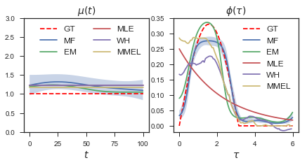
(a)

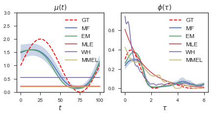
(b)

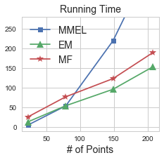
(c)

Figure 1: The fictitious data experimental results. (a): The estimated $\hat{\mu}(t)$ and $\hat{\phi}(\tau)$ in case 1 (with shading being one standard deviation for MF); (b): for case 2. We can see both EM and MF algorithms capture the structure of underlying rates better than other alternatives. (c): The running time (seconds) of different iterative nonparametric algorithms on varying $\#$ of observations. We can see EM and MF algorithms scale linearly with observation, which is more efficient than MMEL. (GT=Ground Truth)

6 Experiments

We evaluate the performance of our proposed EM and mean-field (MF) algorithms on both fictitious and real-world data. Specifically, we compare our proposed algorithms to the following alternatives. 1. Maximum Likelihood Estimation (MLE): the vanilla Hawkes process with constant $\mu$ and exponential decay triggering kernel; 2. Wiener-Hopf (WH): a nonparametric algorithm for Hawkes process where $\mu$ is constant and $\phi(\tau)$ is a nonparametric function (?); 3. Majorization Minimization Euler-Lagrange (MMEL): another nonparametric algorithm for Hawkes process with constant $\mu$ and smooth $\phi(\tau)$, which similarly utilizes the branching structure and estimates $\phi(\tau)$ by an Euler-Lagrange equation (?). We also tried to compare to the long short-term memory (LSTM) based neural Hawkes process (?) but found it hard to converge at least on our data. On the contrary, our proposed algorithms are easier to converge due to the fact that there are fewer parameters to tune, which constitutes another advantage.

We use the following metrics to evaluate the performance of various methods: TestLL: the log-likelihood of hold-out data using the trained model. This is a metric describing the model prediction ability. EstErr: the mean squared error between the estimated $\hat{\mu}(t)$, $\hat{\phi}(\tau)$ and the ground truth. It is only used for fictitious data. RunTime: the running time of various methods w.r.t. the number of training data. Q-Q plot: the plot visualizes the goodness-of-fit for different models using time rescaling theorem (?).

Table 1: EstErr and TestLL for fictitious and real datasets.

		MLE	WH	MMEL	EM	MF
Case 1	$\textit{EstErr}(\hat{\mu},\mu)$	0.236	0.228	0.173	0.137	0.223
	$\textit{EstErr}(\hat{\phi},\phi)$	0.0289	0.0039	0.0053	0.0016	0.0005
	TestLL	31.21	33.72	32.78	33.87	33.98
Case 2	$\textit{EstErr}(\hat{\mu},\mu)$	1.141	0.706	1.135	0.134	0.099
	$\textit{EstErr}(\hat{\phi},\phi)$	0.0076	0.0086	0.0082	0.0011	0.0020
	TestLL	27.48	22.97	26.35	33.18	32.58
Collision	TestLL	420.41	439.67	470.56	470.34	494.46
Crime	TestLL	371.59	400.36	381.42	520.22	375.29

6.1 Fictitious Data Experiments

In fictitious data experiments, we use the thinning algorithm (?) to generate 100 sets of training data and 10 sets of hold-out data with $T_{\phi}=6$ and $T=100$ in 2 cases: 1. $\mu(t)$ is a constant and 2. $\mu(t)$ is changing over time.

1. $\mu(t)=1$ and $\phi(\tau)=\left\{\begin{aligned} &0.33\sin{\tau}\ \ (0<\tau\leq\pi)\\ &0\ \ (\pi<\tau<T_{\phi})\end{aligned}\right.$;

2. $\mu(t)=\sin\left(\frac{2\pi}{T}\cdot t\right)+1\ \ (0<t<T)$ and $\phi(\tau)=0.3\left(\sin(\frac{2\pi}{3}\cdot\tau)+1\right)\cdot\exp(-0.7\tau)\ \ (0<\tau<T_{\phi})$.

The inducing points and hyperparameters are optimized for inference. The estimated $\hat{\mu}(t)$ and $\hat{\phi}(\tau)$ are shown in Fig.1(a) and 1(b). From accuracy perspective, the result in Tab.1 confirms that EM and MF algorithms outperform other alternatives in all cases w.r.t. TestLL and EstErr (mean for MF). For MLE, the estimated results are far away from ground truth due to parametric constraint. For WH and MMEL, the constant limitation on $\mu(t)$ still exists even though $\phi(\tau)$ has been relieved. On the contrary, our EM and MF algorithms provide nonparametric $\hat{\mu}(t)$ and $\hat{\phi}(\tau)$ concurrently. From efficiency perspective, EM and MF algorithms are compared to the other iterative nonparametric algorithm MMEL with same iterations. We can see EM and MF’s RunTime scales linearly with observation in Fig.1(c), which proves their superior efficiency.

6.2 Real Data Experiments

In the real data section, we apply our EM and MF algorithms to two different datasets,

Motor Vehicle Collisions in New York City : a vehicle collision dataset from New York City Police Department;

Crime in Vancouver: a dataset of crimes in Vancouver from the Vancouver Open Data Catalogue.

More experimental details (e.g. dataset introduction, data pre-processing, hyperparameter selection) are provided in Appendix V. We compare the performance of our proposed algorithms to other alternatives. For each inference algorithm, we evaluate its predictive performance using TestLL. The TestLL of EM, MF and other alternatives are shown in Tab.1. We can observe our EM and MF algorithms’ consistent superiority over other alternatives whose baseline intensity or triggering kernel is too restricted to capture the dynamics. To further measure the performance, we generate the Q-Q plot. We transform a sequence of timestamps in hold-out data by the fitted model to a set of independent uniform random variables on the interval $(0,1)$. The result is shown in Appendix V. All experimental results prove our proposed algorithms can not only describe $\mu(t)$ and $\phi(\tau)$ in a completely flexible manner which leads to better goodness-of-fit but also with superior efficiency.

7 Conclusions

In this paper, the scalable EM and mean-filed variational inference algorithms are proposed for sigmoid Gaussian Hawkes process. By augmenting the branching structure, Pólya-Gamma random variables and latent marked Poisson processes, the inference can be performed in a conjugate way efficiently. Furthermore, by introducing sparse GP approximation, our proposed algorithms scale linearly with the number of observations. The fictitious and real data experimental results confirm that the performance of accuracy and efficiency of our proposed algorithms is superior to other state-of-the-art alternatives. Future work can be done on the extension to multivariate or multidimensional Hawkes processes.

Appendix A Appendices

I Proof of Transformation of Sigmoid Function

? (?) found that the inverse hyperbolic cosine can be expressed as an infinite mixture of Gaussian densities

$$\cosh^{-b}{(z/2)}=\int_{0}^{\infty}e^{-z^{2}\omega/2}p_{\text{PG}}(\omega|b,0)d\omega,$$ (1)

where $p_{\text{PG}}(\omega|b,0)$ is the Pólya-Gamma distribution with $\omega\in\mathbb{R}^{+}$. As a result, the sigmoid function can be defined as a Gaussian representation

$$\sigma(z)=\frac{e^{z/2}}{2\cosh{(z/2)}}=\int_{0}^{\infty}e^{h(\omega,z)}p_{\text{PG}}(\omega|1,0)d\omega,$$ (2)

where $h(\omega,z)=z/2-z^{2}\omega/2-\log 2$. This proves Eq.(4) in the main paper.

II Campbell’s Theorem

Let $\Pi_{\hat{\mathcal{Z}}}=\{(\mathbf{z}_{n},\bm{\omega}_{n})\}_{n=1}^{N}$ be a marked Poisson process on the product space $\hat{\mathcal{Z}}=\mathcal{Z}\times\Omega$ with intensity $\Lambda(\mathbf{z},\bm{\omega})=\Lambda(\mathbf{z})p(\bm{\omega}|\mathbf{z})$. $\Lambda(\mathbf{z})$ is the intensity for the unmarked Poisson process $\{\mathbf{z}_{n}\}_{n=1}^{N}$ with $\bm{\omega}_{n}\sim p(\bm{\omega}_{n}|\mathbf{z}_{n})$ being an independent mark drawn at each $\mathbf{z}_{n}$. Furthermore, we define a function $h(\mathbf{z},\bm{\omega}):\mathcal{Z}\times\Omega\rightarrow\mathbb{R}$ and the sum $H(\Pi_{\hat{\mathcal{Z}}})=\sum_{(\mathbf{z},\bm{\omega})\in\Pi_{\hat{\mathcal{Z}}}}h(\mathbf{z},\bm{\omega})$. If $\Lambda(\mathbf{z},\bm{\omega})<\infty$, then

$$\mathbb{E}_{\Pi_{\hat{\mathcal{Z}}}}\left[\exp{\left(\xi H(\Pi_{\hat{\mathcal{Z}}})\right)}\right]$$

$$=\exp{\left[\int_{\hat{\mathcal{Z}}}\left(e^{\xi h(\mathbf{z},\bm{\omega})}-1\right)\Lambda(\mathbf{z},\bm{\omega})d\bm{\omega}d\mathbf{z}\right]},$$

for any $\xi\in\mathbb{C}$. The above equation defines the characteristic functional of a marked Poisson process. This proves Eq.(6) in the main paper. The mean and variance are

$$\mathbb{E}_{\Pi_{\hat{\mathcal{Z}}}}\left[H(\Pi_{\hat{\mathcal{Z}}})\right] =\int_{\hat{\mathcal{Z}}}h(\mathbf{z},\bm{\omega})\Lambda(\mathbf{z},\bm{\omega})d\bm{\omega}d\mathbf{z}$$

$$\text{Var}_{\Pi_{\hat{\mathcal{Z}}}}\left[H(\Pi_{\hat{\mathcal{Z}}})\right] =\int_{\hat{\mathcal{Z}}}[h(\mathbf{z},\bm{\omega})]^{2}\Lambda(\mathbf{z},\bm{\omega})d\bm{\omega}d\mathbf{z}$$

III Proof of Augmented Likelihood

Substituting Eq.(4) and (6) into Eq.(3) in the main paper, we obtain the augmented joint likelihood of baseline intensity part

$$p(D,\mathbf{X}_{ii}|\lambda^{*}_{\mu},f)$$

$$=\prod_{i=1}^{N}\left(\lambda^{*}_{\mu}\sigma(f(t_{i}))\right)^{x_{ii}}\exp{\left(-\int_{T}\lambda^{*}_{\mu}\sigma(f(t))dt\right)}$$

$$=\prod_{i=1}^{N}\left(\int_{0}^{\infty}\lambda^{*}_{\mu}e^{h(\omega_{ii},f(t_{i}))}p_{\text{PG}}(\omega_{ii}|1,0)d\omega_{ii}\right)^{x_{ii}}\cdot$$

$$\mathbb{E}_{p_{\lambda_{\mu}}}\left[\prod_{(\omega_{\mu},t)\in\Pi_{\mu}}e^{h(\omega_{\mu},-f(t))}\right]$$

$$=\iint\prod_{i=1}^{N}\left(\lambda_{\mu}(t_{i},\omega_{ii})e^{h(\omega_{ii},f(t_{i}))}\right)^{x_{ii}}$$

$$\cdot p_{\lambda_{\mu}}(\Pi_{\mu}|\lambda^{*}_{\mu})\prod_{(\omega_{\mu},t)\in\Pi_{\mu}}e^{h(\omega_{\mu},-f(t))}d\bm{\omega}_{ii}d\Pi_{\mu}.$$

with $\bm{\omega}_{ii}$ denoting a vector of $\omega_{ii}$ and $\lambda_{\mu}(t_{i},\omega_{ii})=\lambda^{*}_{\mu}p_{\text{PG}}(\omega_{ii}|1,0)$. Therefore, the augmented joint likelihood is

$$p(D,\Pi_{\mu},\bm{\omega}_{ii},\mathbf{X}_{ii}|\lambda^{*}_{\mu},f)=\prod_{i=1}^{N}\left(\lambda_{\mu}(t_{i},\omega_{ii})e^{h(\omega_{ii},f(t_{i}))}\right)^{x_{ii}}$$

$$\cdot p_{\lambda_{\mu}}(\Pi_{\mu}|\lambda^{*}_{\mu})\prod_{(\omega_{\mu},t)\in\Pi_{\mu}}e^{h(\omega_{\mu},-f(t))}$$

This proves Eq.(7) in the main paper. The proof of Eq.(8) in the main paper is the same and omitted here.

IV Derivation of Mean-field Approach

A standard derivation in the variational mean–field approach shows that the optimal distribution for each factor maximizing the ELBO is given by

$$\log q_{1}(\Pi_{\mu},\bm{\omega}_{ii},\{\Pi_{\phi_{i}}\}_{i=1}^{N},\bm{\omega}_{ij},\mathbf{X})=$$ (3)

$$\mathbb{E}_{q_{2}}[\log p(\Pi_{\mu},\bm{\omega}_{ii},\{\Pi_{\phi_{i}}\}_{i=1}^{N},\bm{\omega}_{ij},\mathbf{X},\lambda^{*}_{\mu},f,\lambda^{*}_{\phi},g)]+C_{1}$$

$$\log q_{2}(\lambda^{*}_{\mu},f,\lambda^{*}_{\phi},g)=$$

$$\mathbb{E}_{q_{1}}[\log p(\Pi_{\mu},\bm{\omega}_{ii},\{\Pi_{\phi_{i}}\}_{i=1}^{N},\bm{\omega}_{ij},\mathbf{X},\lambda^{*}_{\mu},f,\lambda^{*}_{\phi},g)]+C_{2}$$

For our problem, incorporating priors of $\lambda^{*}_{\mu}$, $f$, $\lambda^{*}_{\phi}$ and $g$ into Eq. (7) and (8) in the main paper, we obtain the joint distribution over all variables. Without loss of generality, an improper prior $p(\lambda_{\cdot}^{*})=1/\lambda_{\cdot}^{*}$ and a symmetric GP prior $\mathcal{GP}(\cdot|0,K_{\cdot})$ (?) are utilized here. The final augmented joint distribution of baseline intensity part is

$$p(D, \Pi_{\mu},\bm{\omega}_{ii},\mathbf{X}_{ii},\lambda^{*}_{\mu},f)=\prod_{i=1}^{N}\left(\lambda_{\mu}(t_{i},\omega_{ii})e^{h(\omega_{ii},f(t_{i}))}\right)^{x_{ii}}$$ (4)

$$\cdot p_{\lambda_{\mu}}(\Pi_{\mu}|\lambda^{*}_{\mu})\prod_{(\omega_{\mu},t)\in\Pi_{\mu}}e^{h(\omega_{\mu},-f(t))}\cdot{\lambda_{\mu}^{*}}^{-1}\mathcal{GP}(f);$$

and that of triggering kernel part is

$$p(D,\{\Pi_{\phi_{i}}\}_{i=1}^{N},\bm{\omega}_{ij},\mathbf{X}_{ij},\lambda^{*}_{\phi},g)=$$ (5)

$$\prod_{i=2}^{N}\prod_{j=1}^{i-1}\left(\lambda_{\phi}(\tau_{ij},\omega_{ij})e^{h(\omega_{ij},g(\tau_{ij}))}\right)^{x_{ij}}\cdot$$

$$\prod_{i=1}^{N}\left[p_{\lambda_{\phi}}(\Pi_{\phi_{i}}|\lambda^{*}_{\phi})\prod_{(\omega_{\phi},\tau)\in\Pi_{\phi_{i}}}e^{h(\omega_{\phi},-g(\tau))}\right]\cdot{\lambda_{\phi}^{*}}^{-1}\mathcal{GP}(g).$$

Substituting Eq.(4) and (5) into Eq.(3), we can obtain the optimal distribution for each factor (Eq.(21)$\sim$(25) in the main paper). What is worth noting is that $\bm{\omega}_{ii}$ and $\bm{\omega}_{ij}$ are coupled with branching structure $\mathbf{X}$. We marginalize out $\bm{\omega}$ when solving $q_{1}(\mathbf{X})$ and vice versa.

V Experimental Details

In this appendix, we elaborate on the details of data generation, processing, hyperparameter setup and some experimental results.

Fictitious Data Experimental Details

The first case has a constant $\mu(t)$ and half sinusoidal triggering kernel $\phi(\tau)$. The bandwidth of WH is set to 0.3 and there are 10 inducing points on both $\mu(t)$ and $\phi(\tau)$ for EM and MF. The learned results in Fig.1 and Tab.1 prove EM and MF can learn the correct triggering kernel in non-monotonic decreasing cases.

The second case is a general case with time-changing $\mu(t)$ and sinusoidal exponential decay triggering kernel. The bandwidth of WH is 0.1 and there are 10 inducing points on both $\mu(t)$ and $\phi(\tau)$ for EM and MF. Learned results in Fig.1 and Tab.1 show our proposed algorithms are still the champion.

Vehicle Collision Dataset

In daily transportation, car collisions happening in the past will have a triggering influence on the future because of the traffic congestion caused by the initial accident, so there is a self-exciting phenomenon in this kind of application. The vehicle collision dataset is from New York City Police Department. We filter out weekday records in nearly one month (Sep.18th-Oct.13th 2017). The number of collisions in each day is about 600. Records in Sep.18th-Oct.6th are used as training data and Oct.9th-13th are held out as test data.

We compare the performance of EM, MF and other alternatives. The whole observation period $T$ is set to 1440 minutes (24 hours) and the support of triggering kernel $T_{\phi}$ is set to 60 minutes. For hyperparameters, the bandwidth of WH is set to 0.3 and there are 10 inducing points on $\mu(t)$ and $\phi(\tau)$ for EM and MF with hyperparameters $\{\theta_{0},\theta_{1}\}$ optimized for inference. The final result is the average of learned $\mu(t)$ or $\phi(\tau)$ of each day.

Crime in Vancouver

In crime domain, the past crime will have a triggering effect on future ones, which has been reported in a lot of literature. The data of crimes in Vancouver comes from the Vancouver Open Data Catalogue. It was extracted on 2017-07-18 and it includes all valid felony, misdemeanour and violation crimes from 2003-01-01 to 2017-07-13. The columns are crime type, year, month, day, hour, minute, block, neighbourhood, latitude, longitude etc. We filter out the crime records from 2016-06-01 to 2016-08-31 as training data and 2016-09-01 to 2016-11-30 as test data, add a small time interval to separate all the simultaneous records and delete some records with empty values.

The whole observation period $T$ is set to 92 days and the support of $\phi(\tau)$ is set to 6 days. For hyperparameters, the bandwidth of WH is set to 0.5 and there are still 10 inducing points on $\mu(t)$ and $\phi(\tau)$ for EM and MF with hyperparameters $\{\theta_{0},\theta_{1}\}$ optimized for inference.

Q-Q plot

After the baseline intensity and triggering kernel estimated from the training data series, we can compute the rescaled timestamps of test data:

$$\tau_{i}=\Lambda(t_{i})-\Lambda(t_{i-1}),$$

where $\Lambda(t_{i})=\int_{0}^{t_{i}}\lambda(t|\mathcal{H}_{t_{i}})dt$, $\mathcal{H}_{t_{i}}$ is the history before $t_{i}$. According to the time rescaling theorem, $\{\tau_{i}\}$ are independent exponential random variables with mean $1$ if the model is correct. With further transformation:

$$z_{i}=1-\exp(-\tau_{i}),$$

$\{z_{i}\}$ are independent uniform random variables on the interval $(0,1)$. Any statistical assessment that measures agreement between the transformed data and a uniform distribution evaluates how well the fitted model agrees with the test data. So we can draw the Q-Q plot of the transformed timestamps with respect to the uniform distribution. The plots are shown in Fig. 2. The perfect model follows a straight line of $y=x$. We can observe that the learned model from our algorithm (the better one from EM or MF) is generally closer to the straight line, which suggests its better goodness-of-fit.

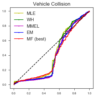
(a)

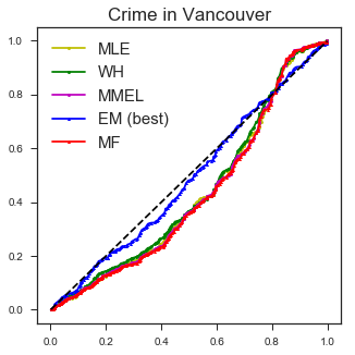
(b)

Figure 2: Q-Q plot of EM, MF and other alternative inference algorithms for the real data.

References

• [Adams, Murray, and MacKay 2009] Adams, R. P.; Murray, I.; and MacKay, D. J. 2009. Tractable nonparametric Bayesian inference in Poisson processes with Gaussian process intensities. In Proceedings of the 26th Annual International Conference on Machine Learning, 9–16. ACM.
• [Bacry and Muzy 2016] Bacry, E., and Muzy, J.-F. 2016. First-and second-order statistics characterization of Hawkes processes and non-parametric estimation. IEEE Transactions on Information Theory 62(4):2184–2202.
• [Bishop 2007] Bishop, C. 2007. Pattern recognition and machine learning (Information Science and Statistics), 1st edn. 2006. corr. 2nd printing edn. Springer, New York.
• [Cunningham, Shenoy, and Sahani 2008] Cunningham, J. P.; Shenoy, K. V.; and Sahani, M. 2008. Fast Gaussian process methods for point process intensity estimation. In Proceedings of the 25th international conference on Machine learning, 192–199. ACM.
• [Daley and Vere-Jones 2003] Daley, D. J., and Vere-Jones, D. 2003. An introduction to the theory of point processes. vol. i. probability and its applications.
• [Donner and Opper 2018] Donner, C., and Opper, M. 2018. Efficient Bayesian inference for a Gaussian process density model. arXiv preprint arXiv:1805.11494.
• [Donner 2019] Donner, C. 2019. Bayesian inference of inhomogeneous point process models.
• [Du et al. 2016] Du, N.; Dai, H.; Trivedi, R.; Upadhyay, U.; Gomez-Rodriguez, M.; and Song, L. 2016. Recurrent marked temporal point processes: embedding event history to vector. In Proceedings of the 22nd ACM SIGKDD International Conference on Knowledge Discovery and Data Mining, 1555–1564. ACM.
• [Eichler, Dahlhaus, and Dueck 2017] Eichler, M.; Dahlhaus, R.; and Dueck, J. 2017. Graphical modeling for multivariate Hawkes processes with nonparametric link functions. Journal of Time Series Analysis 38(2):225–242.
• [Gupta et al. 2018] Gupta, A.; Farajtabar, M.; Dilkina, B.; and Zha, H. 2018. Discrete interventions in Hawkes processes with applications in invasive species management. In IJCAI, 3385–3392.
• [Kingman 2005] Kingman, J. F. C. 2005. Poisson processes. Encyclopedia of biostatistics 6.
• [Lewis and Mohler 2011] Lewis, E., and Mohler, G. 2011. A nonparametric EM algorithm for multiscale Hawkes processes. Journal of Nonparametric Statistics 1(1):1–20.
• [Liu, Yan, and Chen 2018] Liu, Y.; Yan, T.; and Chen, H. 2018. Exploiting graph regularized multi-dimensional Hawkes processes for modeling events with spatio-temporal characteristics. In IJCAI, 2475–2482.
• [Lloyd et al. 2015] Lloyd, C.; Gunter, T.; Osborne, M.; and Roberts, S. 2015. Variational inference for Gaussian process modulated Poisson processes. In International Conference on Machine Learning, 1814–1822.
• [Marsan and Lengline 2008] Marsan, D., and Lengline, O. 2008. Extending earthquakes’ reach through cascading. Science 319(5866):1076–1079.
• [Mei and Eisner 2017] Mei, H., and Eisner, J. M. 2017. The neural Hawkes process: A neurally self-modulating multivariate point process. In Advances in Neural Information Processing Systems, 6754–6764.
• [Møller, Syversveen, and Waagepetersen 1998] Møller, J.; Syversveen, A. R.; and Waagepetersen, R. P. 1998. Log Gaussian Cox processes. Scandinavian journal of statistics 25(3):451–482.
• [Ogata 1998] Ogata, Y. 1998. Space-time point-process models for earthquake occurrences. Annals of the Institute of Statistical Mathematics 50(2):379–402.
• [Papangelou 1972] Papangelou, F. 1972. Integrability of expected increments of point processes and a related random change of scale. Transactions of the American Mathematical Society 165:483–506.
• [Pinto, Chahed, and Altman 2015] Pinto, J. C. L.; Chahed, T.; and Altman, E. 2015. Trend detection in social networks using Hawkes processes. In Proceedings of the 2015 IEEE/ACM International Conference on Advances in Social Networks Analysis and Mining 2015, 1441–1448. ACM.
• [Polson, Scott, and Windle 2013] Polson, N. G.; Scott, J. G.; and Windle, J. 2013. Bayesian inference for logistic models using Pólya-Gamma latent variables. Journal of the American statistical Association 108(504):1339–1349.
• [Rasmussen 2003] Rasmussen, C. E. 2003. Gaussian processes in machine learning. In Summer School on Machine Learning, 63–71. Springer.
• [Reynaud-Bouret, Schbath, and others 2010] Reynaud-Bouret, P.; Schbath, S.; et al. 2010. Adaptive estimation for Hawkes processes; application to genome analysis. The Annals of Statistics 38(5):2781–2822.
• [Samo and Roberts 2015] Samo, Y.-L. K., and Roberts, S. 2015. Scalable nonparametric Bayesian inference on point processes with Gaussian processes. In International Conference on Machine Learning, 2227–2236.
• [Titsias 2009] Titsias, M. 2009. Variational learning of inducing variables in sparse Gaussian processes. In Artificial Intelligence and Statistics, 567–574.
• [Zhou et al. 2018] Zhou, F.; Li, Z.; Fan, X.; Wang, Y.; Sowmya, A.; and Chen, F. 2018. A refined MISD algorithm based on Gaussian process regression. In Pacific-Asia Conference on Knowledge Discovery and Data Mining, 584–596. Springer.
• [Zhou, Zha, and Song 2013] Zhou, K.; Zha, H.; and Song, L. 2013. Learning triggering kernels for multi-dimensional Hawkes processes. In International Conference on Machine Learning, 1301–1309.
• [Zhou 2019] Zhou, F. 2019. Efficient EM-variational inference for Hawkes process. arXiv preprint arXiv:1905.12251.