Ensemble quantile classifier

Abstract

Both the median-based classifier and the quantile-based classifier are useful for discriminating high-dimensional data with heavy-tailed or skewed inputs. But these methods are restricted as they assign equal weight to each variable in an unregularized way. The ensemble quantile classifier is a more flexible regularized classifier that provides better performance with high-dimensional data, asymmetric data or when there are many irrelevant extraneous inputs. The improved performance is demonstrated by a simulation study as well as an application to text categorization. It is proven that the estimated parameters of the ensemble quantile classifier consistently estimate the minimal population loss under suitable general model assumptions. It is also shown that the ensemble quantile classifier is Bayes optimal under suitable assumptions with asymmetric Laplace distribution inputs.
Keywords: Binary classification, Extraneous noise variables, High-dimensional discriminant analysis, Pattern recognition and machine learning, Sparsity, Text mining,

1 Introduction

The class prediction problem with $p$-dimensional input $\bm{x}=(x_{1},\dotsc,x_{p})$ and output variable $y\in{\cal K}$, where ${\cal K}=\{1,\ldots,K\}$, is considered. For each class $k\in{\cal K}$, $\bm{x}$ is a $p$-multivariate random vector generated from the multivariate probability distributions $P_{k}$. The family of component-wise distance-based discriminant rules is defined by,

$$D_{k}=\sum_{j=1}^{p}d(x_{j},P_{k,j}),$$ (1)

where $x_{j}\in\Re$ is a test input, $P_{k,j}$ is the $j$-th marginal distribution of $P_{k}$, and $d(x_{j},P_{k,j})$ is the distance between $x_{j}$ and $P_{k,j}$ (Hennig and Viroli, 2016a; Hall et al., 2009; Tibshirani et al., 2003). The optimal prediction is

$$\hat{y}={\rm argmin}_{k\in{\cal K}}D_{k}.$$ (2)

For example, the centroid classifier may be defined by $d(x_{j},P_{k,j})=(x_{j}-\mu_{k,j})^{2}$ where $\mu_{k,j}$ is the mean of $P_{k,j}$. This classifier is a special case of the naive Bayes classifier (Hastie et al., 2009), also known as the diagonal linear discriminant classifier. It provides an effective classifier for large $p$ and many types of high dimensional data inputs (Dudoit et al., 2002; Bickel and Levina, 2004; Fan and Fan, 2008). When the input $\bm{x}$ includes symmetric random variables with fat tails, the median classifier (MC), $d(x_{j},P_{k,j})=|x_{j}-m_{k,j}|$, where $m_{k,j}={\rm median}(P_{k,j})$, $k\in{\cal K}$ and $j=1,\ldots,p$, often has better performance. Hall et al. (2009) proved that under suitable regularity conditions MC produced asymptotically correct predictions. In practice a training data set, where variables may be rescaled if necessary (Hennig and Viroli, 2016a, Section 4.1), is used to estimate the parameters $\mu_{k,j}$ or $m_{k,j}$ for $k\in{\cal K}$ and $j=1,\ldots,p$.

It sometimes happens that the distribution of two variables is similar near the center but differs in the tails due to skewness or other characteristics. Quantile regression makes use of this phenomenon (Koenker and Bassett, 1978). The Tukey mean difference plot (Cleveland, 1993, p.21) was invented to compare data from such distributions. Hennig and Viroli (2016a) extended MC to the quantile-based classifier (QC) defined by $d(x_{j},P_{k,j})=\rho_{\theta_{j}}(x_{j}-q_{k,j}({\theta_{j}}))$, where $q_{k,j}({\theta_{j}})$ is the $\theta_{j}$-quantile of $P_{k,j}$ for $0<\theta_{j}<1$ and

$$\rho_{\theta}(u)=u(\theta-\mathbf{1}_{\{u<0\}})$$ (3)

is the quantile distance function (Koenker and Bassett, 1978; Koenker, 2005). When $\theta=0.5$, QC reduces to MC. Hennig and Viroli (2016a) showed that the QC can provide the Bayes optimal prediction with skewed input distributions. The usefulness of QC was demonstrated by simulation as well as an application (Hennig and Viroli, 2016a). An R package which implements the centroid, median and quantile classifiers is available (Hennig and Viroli, 2016b).

Although QC is effective for discriminating high-dimensional data with heavy-tailed or skewed inputs, it suffers from the restriction of assigning each variable the same importance, which limits its effectiveness when there are irrelevant extraneous inputs. Another limitation for QC and the median centroid classifier with high dimensional data may be noise accumulation. Fan and Fan (2008, Theorem 1a) proved that the centroid classifier may perform no better than random guessing due to noise accumulation with high dimensional data.

Our proposed ensemble quantile classifier (EQC), presented in Section 2, is a flexible regularized classifier that aims to overcome these two limitations and provides better performance with high-dimensional data, asymmetric data or when there are many irrelevant extraneous inputs. We introduce the binary EQC for discriminating observations into one of two classes and then extend it to situations with more than two classes. In 2 of Section 3, it is shown that sample loss function of EQC converges to the population value when the sample size increases. In Section 4 and Section 5, the improved performance of EQC is demonstrated by a simulation study and an application to text categorization.

2 Ensemble quantile classifier

Ensemble predictors were derived from the idea popularly known as Wisdom of the Crowd (Hastie et al., 2009; Silver, 2012). Newbold and Granger (1974) showed that economic time series forecasts could be improved by using a weighted average of forecasts from a heterogeneous variety of time series models. Many advanced ensemble prediction methods for supervised learning problems have been developed such as random forests (Breiman, 2001) and various boosting algorithms (Freund and Schapire, 1997; Schapire and Freund, 2012). The ensemble stacking method introduced by Wolpert (1992) and Breiman (1996) has also been widely used. Comprehensive surveys of ensemble learning algorithms are given by Hastie et al. (2009); Dietterich (2000); Zhou (2012) and Lior (2019). Ensemble stacking uses a metalearner to combine base learners. In Section 2.1 and Section 2.2 a method for using regularized logistic regression to combine quantile classifiers is developed and is generalized to the multiclass case in Section 2.3.

2.1 Quantile-difference transformation and EQC

For the classification problem with $K$ classes and $p$ inputs, let $q_{k,j}({\theta_{j}})$ be the $\theta_{j}$-quantile of $P_{k,j}$ where $0<\theta_{j}<1$ for $k\in{\cal K}$ and $j=1,\ldots,p$. The derived inputs to the metalearner are obtained from the quantile-difference transformation of $\bm{x}=(x_{1},\dotsc,x_{p})$ defined by,

$$\operatorname{Q}_{\bm{\theta}}^{(k_{1},k_{2})}(\bm{x})=\bigl{(}\operatorname{Q}_{\theta_{1}}^{(k_{1},k_{2})}(x_{1}),\dotsc,\operatorname{Q}_{\theta_{p}}^{(k_{1},k_{2})}(x_{p})\bigr{)},$$ (4)

where,

$$\operatorname{Q}_{\theta_{j}}^{(k_{1},k_{2})}(x_{j})=\rho_{\theta_{j}}(x_{j}-q_{k_{1},j}(\theta_{j}))-\rho_{\theta_{j}}(x_{j}-q_{k_{2},j}(\theta_{j})),\ j=1,\dotsc,p,$$

and $\rho_{\theta}(u)=u(\theta-\mathbf{1}_{\{u<0\}})$ is the quantile-distance function. The superscript $(k_{1},k_{2})$ is omitted if $k_{1}=1$ and $k_{2}=2$. As shown in Figure 1 the quantile-difference transformation has constant tails so the derived inputs are insensitive to outliers.

Figure 1: Quantile-difference transformation for classes 1 and 2 when $q_{1}(\theta)<q_{2}(\theta)$.

In the binary case, the QC discriminant function is given by $s(\bm{x}\mid\bm{\theta})=\sum_{j}\operatorname{Q}_{\theta_{j}}(x_{j})$ where $\bm{x}=(x_{1},\ldots,x_{p})$ is a test input and $\bm{\theta}=(\theta_{1},\ldots,\theta_{p})$. The classifier predicts class 1 or 2 according as $s(\bm{x}\mid\bm{\theta})\leqslant 0$ or $>0$. Hennig and Viroli (2016a) estimated the parameter $\bm{\theta}$ by minimizing the misclassification rate on the training data using a grid search. In most cases they found that using the same value of $\theta_{j}=\theta$, $j=1,\dotsc,p$ for all input variables worked well for the QC, which means a restriction $\bm{\theta}=\{\theta,\dotsc,\theta\}\in\bm{\Theta}\subseteq(0,1)^{p}$. For simplicity and computational expediency, this restriction was imposed in the simulation study and the application to text categorization.

2.2 EQC for binary case

The discriminant function for QC is simply an additive sum $\operatorname{Q}_{\theta_{j}}(x_{j})$ for $j=1,\dotsc,p$ but in practice it is often the case that several of the variables are more important and should be given more weights. EQC is proposed to extend QC by providing an effective classifier that takes this into account. The discriminate function for the EQC binary case may be written,

$$s(\bm{x}\mid\bm{\theta},\beta_{0},\bm{\beta})=\mathsf{C}\bigl{(}\operatorname{Q}_{\bm{\theta}}(\bm{x})\mid\beta_{0},\bm{\beta}\bigr{)},$$ (5)

where $\operatorname{Q}_{\bm{\theta}}(\bm{x})$ is defined in Equation 4 and $\mathsf{C}(\bm{z}\mid\beta_{0},\bm{\beta})$ is the metalearner with the intercept term $\beta_{0}\in\mathbb{R}$ and the weight vector $\bm{\beta}\in\mathbb{R}^{p}$. Then $(\beta_{0},\bm{\beta})$ along with the $p$ quantile parameters $\bm{\theta}\in(0,1)^{p}$ may be estimated by minimizing a suitable regularized loss function with a regularization parameter $\bm{\alpha}$ using cross-validation.

The metalearner $\mathsf{C}(\bm{z}\mid\beta_{0},\bm{\beta})$ can be substituted by the discriminant function of most regularized classifiers such as the penalized logistic regression (Park and Hastie, 2007) or the support vector machine (SVM) (Cortes and Vapnik, 1995). For the penalized logistic regression $\bm{\alpha}=\lambda$, where $\lambda$ is the penalty defined in Equation 7 while for the SVM model with the linear kernel defined in Equation 8, $\bm{\alpha=}\mathfrak{c}$, where $\mathfrak{c}$ is the cost penalty. Ridge logistic regression is recommended as a default choice for $\mathsf{C}$ since it often performs well. For high-dimensional data where $p>n$, it is preferable to treat $\bm{\theta}$ as a tuning parameter and estimate it together with $\bm{\alpha}$ using cross-validation to avoid overfitting.

When the quantiles are substituted by their estimates, the estimated discriminant function is denoted by $\hat{\mathcal{G}}(\bm{x}\mid\bm{\theta},\beta_{0},\bm{\beta})$ and the estimated quantile-difference transformation is denoted by $\hat{\operatorname{Q}}_{\bm{\theta}}(\bm{x}_{i})$.

Using the penalized logistic regression for $\mathsf{C}$,

$$\mathsf{C}\bigl{(}\operatorname{Q}_{\bm{\theta}}(\bm{x})\mid\beta_{0},\bm{\beta}\bigr{)}=\beta_{0}+\sum_{j=1}^{p}\beta_{j}\operatorname{Q}_{\theta_{j}}(x_{j}).$$ (6)

Let $\bm{\alpha}=\lambda$ be the penalty parameter in the regularized binomial loss function (Friedman et al., 2010). So given $\lambda$ and the input $\operatorname{Q}_{\bm{\theta}}(\bm{x})$, $(\beta_{0},\bm{\beta})$ may be estimated by minimizing,

$$\text{Loss}_{\text{binomial}}\Bigl{(}\beta_{0},\bm{\beta}\bigm{|}\lambda,\operatorname{Q}_{\bm{\theta}}(\bm{x}_{i}),i=1,\dotsc,n\Bigr{)}= -\frac{1}{n}\sum_{i=1}^{n}\Bigl{\{}(y_{i}-1)\mathsf{C}\bigl{(}\operatorname{Q}_{\bm{\theta}}(\bm{x}_{i})\mid\beta_{0},\bm{\beta}\bigr{)}-$$

$$\log(1+e^{\mathsf{C}(\operatorname{Q}_{\bm{\theta}}(\bm{x}_{i})\mid\beta_{0},\bm{\beta})})\Bigr{\}}+\frac{\lambda}{2}\lVert\bm{\beta}\rVert_{l},$$ (7)

where $\lVert\bm{\beta}\rVert_{1}=\sum_{j=1}^{p}|\beta_{j}|$ for LASSO and $\lVert\bm{\beta}\rVert_{2}=\sum_{j=1}^{p}\beta_{j}^{2}$ for ridge regression. Using the SVM with the linear kernel (LSVM) has the same linear discriminant function as Equation 6, but $(\beta_{0},\bm{\beta})$ is estimated by minimizing the regularized hinge loss (Hastie et al., 2009, Equation 12.25),

$$\text{Loss}_{\text{hinge}}\Bigl{(}\beta_{0},\bm{\beta}\bigm{|}\mathfrak{c},\operatorname{Q}_{\bm{\theta}}(\bm{x}_{i}),i=1,\dotsc,n\Bigr{)}= \frac{1}{n}\sum_{i=1}^{n}\Bigl{[}1-(y_{i}-1)\mathsf{C}\bigl{(}\operatorname{Q}_{\bm{\theta}}(\bm{x}_{i})\mid\beta_{0},\bm{\beta}\bigr{)}\Bigr{]}_{+}+\frac{1}{2n\mathfrak{c}}\lVert\bm{\beta}\rVert_{2},$$ (8)

where $[x]_{+}$ indicates the positive part of $x$ and $\mathfrak{c}$ is the cost tuning parameter.

If $\beta_{0}=0$ and $\beta_{j}=1$ for $j=1,\dotsc,p$, then EQC has the same decision boundary as QC. In A, it is shown that EQC with $\mathsf{C}$ defined in Equation 6 has the same form as the Bayes decision boundary when $P_{1}$ and $P_{2}$ consist of independent asymmetric Laplace distributions. This motivates further exploration and development of the EQC. The estimation of $(\beta_{0},\bm{\beta})$ by ridge/LASSO penalized logistic regression and LSVM are all capable of dealing with high dimensional data. The associated ensemble classifiers used in this paper are denoted respectively by EQC/RIDGE, EQC/LASSO and EQC/LSVM. A non-negative constraint of $\bm{\beta}$ was also investigated but we did not find an experimentally significant accuracy improvement, which agrees with a previous study of stacking classifiers (Ting and Witten, 1999).

Algorithm 1 shows the entire process of tuning and training EQC. Here the misclassification rate is used as a criterion to choose the tuning parameters but in some cases other criteria such as the AUC may be appropriate.

The time complexity of this algorithm is determined by the time complexities for the quantile estimation, the quantile-difference transformation and the coordinate descent algorithm which are respectively $O\bigl{(}pn\log(n)\bigr{)}$, $O(npH)$, $O\bigl{(}n(p+1)IH)\bigr{)}$, where $H$ is the size of the tuning set $\bm{\Theta}$, and $I$ is the number of iterations required for minimization of the loss function. In total Algorithm 1 has complexity $O\bigl{(}(T+1)(pn\log(n)+n(p+1)IH)\bigr{)}$, where $T$ is the number of cross-validation folds. The computational burden for cross-validation may be reduced by using parallel computation (Kuhn and Johnson, 2013).

Data: $S=\{(\bm{x}_{1},y_{1}),\dotsc,(\bm{x}_{n},y_{n})\}$, $p=$ the number of variables within $\bm{x}$.

Input: $\bm{\Theta}=$ tuning set of $\bm{\theta}\in(0,1)^{p}$, $\mathbb{A}=$ tuning set of $\bm{\alpha}$, $T=$ the number of cross-validation folds.

begin tuning parameters:

       Randomly partition $S$ into $T$ non-overlap folds, $S_{1},\dotsc,S_{T}$.

       for $t=1,\dotsc,T$ do fit $\mathsf{C}$ on $S\setminus S_{t}$,

             foreach $\bm{\theta}$ in $\bm{\Theta}$ do

                   Estimate $\hat{q}_{k,j}(\theta_{j})$ for $k=1,2$ and $j=1,\dotsc,p$ from $S\setminus S_{t}$.

                   Compute $\hat{\operatorname{Q}}_{\bm{\theta}}(\bm{x}_{i})$ for $i=1,\dotsc,n$.

                   foreach  $\bm{\alpha}$ in $\mathbb{A}$  do

                         Estimate $(\beta_{0},\bm{\beta})$ by minimizing the loss function such as Equation 7 on $\hat{\operatorname{Q}}_{\bm{\theta}}(\bm{x}_{i})$ for $(\bm{x}_{i},y_{i})\in S\setminus S_{t}$ with the tuning parameter $\bm{\alpha}$.

                         Apply the estimated $\hat{\mathsf{C}}$ on $\hat{\operatorname{Q}}_{\bm{\theta}}(\bm{x}_{i})$ for $(\bm{x}_{i},y_{i})\in S_{t}$ and return the misclassification rates.

                   end foreach

                  

             end foreach

            

       end for

      Average the misclassification rate over folds for each combination of $\bm{\theta}$ and $\bm{\alpha}$. Denote $(\hat{\bm{\theta}},\hat{\bm{\alpha}})$ as the combination with the minimum average misclassification rate.

      

end

Output: Refit $\mathsf{C}$ with $(\hat{\bm{\theta}},\hat{\bm{\alpha}})$ on the full data $S$.

Algorithm 1 Tune and train EQC for binary case

2.3 Multiclass EQC

A practical method to extend the binary classifier to multiclass ($K>2$) is to build a set of one-versus-all classifiers or a set of one-versus-one classifiers (Hastie et al., 2009, p. 658). A less heuristic approach, similar to the multinomial logistic regression, is to use the $K-1$ log-odd-ratios to implement maximum likelihood estimation (MLE). The multinomial logistic regression requires estimation of $(K-1)(p+1)$ coefficients but here the multiclass EQC only requires $p+K-1$ coefficients including $p$ weights $\beta_{j}$, $j=1,\dotsc,p$, and $K-1$ intercept terms $\beta_{0,k}$, $k=1,\dotsc,K-1$.

Let $\bm{\beta}=(\beta_{1},\dotsc,\beta_{p})$. Assume for an input $\bm{x}$,

$$\log\frac{\mathbb{P}(y=1\mid\bm{x},\bm{\theta},\bm{\beta},\{\beta_{0,k}\}_{k=1}^{K-1})}{\mathbb{P}(y=K\mid\bm{x},\bm{\theta},\bm{\beta},\{\beta_{0,k}\}_{k=1}^{K-1})} =-\mathsf{C}\bigl{(}\operatorname{Q}_{\bm{\theta}}^{(1,K)}(\bm{x})\mid\beta_{0,1},\bm{\beta}\bigr{)}$$

$$\log\frac{\mathbb{P}(y=2\mid\bm{x},\bm{\theta},\bm{\beta},\{\beta_{0,k}\}_{k=1}^{K-1})}{\mathbb{P}(y=K\mid\bm{x},\bm{\theta},\bm{\beta},\{\beta_{0,k}\}_{k=1}^{K-1})} =-\mathsf{C}\bigl{(}\operatorname{Q}_{\bm{\theta}}^{(2,K)}(\bm{x})\mid\beta_{0,2},\bm{\beta}\bigr{)}$$

$$\vdots$$

$$\log\frac{\mathbb{P}(y=K-1\mid\bm{x},\bm{\theta},\bm{\beta},\{\beta_{0,k}\}_{k=1}^{K-1})}{\mathbb{P}(y=K\mid\bm{x},\bm{\theta},\bm{\beta},\{\beta_{0,k}\}_{k=1}^{K-1})} =-\mathsf{C}\bigl{(}\operatorname{Q}_{\bm{\theta}}^{(K-1,K)}(\bm{x})\mid\beta_{0,K-1},\bm{\beta}\bigr{)},$$

and $\sum_{k=1}^{K}\mathbb{P}(y=k\mid\bm{x},\bm{\theta},\bm{\beta},\{\beta_{0,k}\}_{k=1}^{K-1})=1$. The negative sign prior to $\mathsf{C}$ is used because class $K$ is used in the denominator of the log-odd-ratios and it is the alternative class in $\operatorname{Q}_{\bm{\theta}}^{(k,K)}(\bm{x})$, which implies that the smaller $\mathsf{C}\bigl{(}\operatorname{Q}_{\bm{\theta}}^{(k,K)}(\bm{x})\mid\beta_{0,k},\bm{\beta}\bigr{)}$ is, the closer $\bm{x}$ is to class $k$ compared to class $K$ and hence the larger the log-odd-ratios between class $k$ and class $K$ is. Let $\beta_{0,K}=0$ and thus,

$$\mathbb{P}(y=k_{0}\mid\bm{x},\bm{\theta},\bm{\beta},\{\beta_{0,k}\}_{k=1}^{K-1})=\frac{e^{-\mathsf{C}\bigl{(}\mathopen{}\mathclose{{}\left.\operatorname{Q}_{\bm{\theta}}^{(k_{0},K)}(\bm{x})}\right|\,\beta_{0,k_{0}},\bm{\beta}\bigr{)}}}{\sum_{k=1}^{K}e^{{-\mathsf{C}\bigl{(}\mathopen{}\mathclose{{}\left.\operatorname{Q}_{\bm{\theta}}^{(k,K)}(\bm{x})}\right|\,\beta_{0,k},\bm{\beta}\bigr{)}}}},\text{ for }k_{0}=1,\dotsc,K.$$ (9)

Given the tuning parameter $\lambda$, the L2 regularized log-likelihood function may be written,

$$\tilde{\ell}(\bm{\beta},\{\beta_{0,k}\}_{k=1}^{K-1}\mid\bm{\theta},\lambda)=\frac{1}{n}\sum_{i=1}^{n}\log\mathbb{P}(y=y_{i}\mid\bm{x}_{i},\bm{\theta},\bm{\beta},\{\beta_{0,k}\}_{k=1}^{K-1})-\frac{\lambda}{2}\sum_{j=1}^{p}\beta_{j}^{2}.$$ (10)

It can be shown that $\tilde{\ell}(\bm{\beta},\{\beta_{0,k}\}_{k=1}^{K-1}\mid\bm{\theta},\lambda)$ is a concave function so it is amenable to optimization based on gradients or Newton’s method. For further details see B and the software implementation (Lai and McLeod, 2018).

3 Asymptotic consistency

In this section, the theoretical result is derived in a slightly modified setup of the method in Algorithm 1. It is assumed that $p$ is fixed while $n$ increases, so $\bm{\theta}$ and $(\beta_{0},\bm{\beta})$ may be estimated by maximum likelihood. In addition, $\bm{\alpha}$ is neglected as the asymptotic properties of the selection of the tuning parameter are not discussed.

Let $(\tilde{\bm{\theta}},\tilde{\beta}_{0},\tilde{\bm{\beta}})$ be the parameters that minimize the population binomial loss function,

$$\Psi(\bm{\theta},\beta_{0},\bm{\beta}) =\pi_{1}\int\log(1+e^{\mathsf{C}(\operatorname{Q}_{\bm{\theta}}(\bm{x})\mid\beta_{0},\bm{\beta})})\mathop{}\!\mathrm{d}P_{1}(\bm{x})-$$

$$\phantom{==}\pi_{2}\int\Bigl{\{}\mathsf{C}\bigl{(}\operatorname{Q}_{\bm{\theta}}(\bm{x})\mid\beta_{0},\bm{\beta}\bigr{)}-\log(1+e^{\mathsf{C}(\operatorname{Q}_{\bm{\theta}}(\bm{x})\mid\beta_{0},\bm{\beta})})\Bigr{\}}\mathop{}\!\mathrm{d}P_{2}(\bm{x}),$$ (11)

where $\pi_{1}$ and $\pi_{2}$ are prior probabilities of the two classes.

Let $(\hat{\bm{\theta}}_{n},\hat{\beta}_{n0},\hat{\bm{\beta}}_{n})$ be the parameters that minimize the empirical binomial loss function,

$$\Psi_{n}(\bm{\theta},\beta_{0},\bm{\beta})=-\frac{1}{n}\sum_{i=1}^{n}\Bigl{\{}(y_{i}-1)\mathsf{C}\bigl{(}\hat{\operatorname{Q}}_{\bm{\theta}}(\bm{x}_{i})\mid\beta_{0},\bm{\beta}\bigr{)}-\log(1+e^{\mathsf{C}(\hat{\operatorname{Q}}_{\bm{\theta}}(\bm{x}_{i})\mid\beta_{0},\bm{\beta})})\Bigr{\}}.$$ (12)

It is shown that under suitable assumptions, $(\hat{\bm{\theta}}_{n},\hat{\beta}_{n0},\hat{\bm{\beta}}_{n})$ is a consistent estimator of $(\tilde{\bm{\theta}},\tilde{\beta}_{0},\tilde{\bm{\beta}})$. The proofs are available in C. These results have been proved by Hennig and Viroli (2016a) for the quantile-based classifier with the 0-1 loss function. The proof given by them has been adapted to take into account the additional parameters $(\beta_{0},\bm{\beta})$ and the change of the loss function from the 0-1 loss function to the binomial loss function. Assumption 2 is added in addition to Assumption 1 made by Hennig and Viroli (2016a). The linear discriminant function or metalearner $\mathsf{C}(\bm{z}\mid\beta_{0},\bm{\beta})$ in Equation 6, the discriminant function with multiplicative interactions, and the polynomial discriminant function used in polynomial kernel SVM all satisfy Assumption 2. These assumptions ensure the convergence can still hold with $(\beta_{0},\bm{\beta})$. The use of the binomial loss function simplifies the proof and the computation. Since the 0-1 loss function is not a convex or a continuous function, its minimization is NP-hard and hence the binomial loss function or the hinge loss function are used instead. Assumption 2 of Hennig and Viroli (2016a) is not needed because the binomial loss function is used.

Assumption 1.

$\forall j=1,\dotsc,p$, $k=1,2$, the quantile function $q_{k,j}(\theta_{j})$ is a continuous function of $\theta_{j}\in\Theta_{j}\subset({0},{1})$.

Assumption 2.

$\mathsf{C}(\bm{z}\mid\beta_{0},\bm{\beta})$ is required to be differentiable with respect to $\bm{z}$, $\beta_{0}$ and $\bm{\beta}$. In addition, $\tilde{\beta}_{0}$ and $\tilde{\bm{\beta}}$ are required to be bounded. That is, $\exists C>0$ such that $\lvert\tilde{\beta}_{j}\rvert\leqslant C$, for $j=0,1,\dotsc,p$.

Theorem 1.

Under Assumptions 1 and 2, $\forall\epsilon>0$,

$$\lim_{n\rightarrow\infty}\mathbb{P}\{\lvert\Psi(\tilde{\bm{\theta}},\tilde{\beta}_{0},\tilde{\bm{\beta}})-\Psi(\hat{\bm{\theta}}_{n},\hat{\beta}_{n0},\hat{\bm{\beta}}_{n})\rvert>\epsilon\}=0.$$

Assumption 2 is needed to ensure that the estimation of $(\beta_{0},\bm{\beta})$ converges. 1 shows that the estimated parameters are consistent in achieving the minimal population loss. Beside, 2 states that the empirical minimal loss will converge to the population minimal loss asymptotically as $n\rightarrow\infty$ with $p$ fixed.

Theorem 2.

Under Assumptions 1 and 2, $\forall\epsilon>0$,

$$\lim_{n\rightarrow\infty}\mathbb{P}\{\lvert\Psi(\tilde{\bm{\theta}},\tilde{\beta}_{0},\tilde{\bm{\beta}})-\Psi_{n}(\hat{\bm{\theta}}_{n},\hat{\beta}_{n0},\hat{\bm{\beta}}_{n})\rvert>\epsilon\}=0.$$

Based on 1 and 2, when $n$ is large relative to $p$, Algorithm 1 can be modified to estimate $\theta$ by minimizing the training loss function instead of using cross-validation approach.

4 Simulation validation

4.1 Experimental setup

Simulation experiments are presented to demonstrate the improved performance of EQC over QC with high-dimensional skewed inputs as well as other classifiers. The following thirteen classifiers were compared:

QC

quantile-based classifier (Hennig and Viroli, 2016a);

MC

median-based classifier (Hall et al., 2009);

EMC

EQC with $\theta=0.5$ with ridge logistic regression;

EQC/LOGISTIC

EQC with logistic regression;

EQC/RIDGE

EQC with ridge logistic regression;

EQC/LASSO

EQC with LASSO logistic regression;

EQC/LSVM

EQC with linear SVM;

NB

naive Bayes classifier;

LDA

linear discriminant analysis;

LASSO

LASSO logistic regression (Friedman et al., 2010);

RIDGE

ridge logistic regression (Friedman et al., 2010);

LSVM

SVM with linear kernel (Cortes and Vapnik, 1995);

RSVM

SVM with radial basis kernel (Cortes and Vapnik, 1995).

Tuning parameters were selected by minimizing the 5-fold cross validation errors. QC, MC and EQC were fit using the R implementation (Lai and McLeod, 2018) while NB, LSVM and RSVM used the algorithms in Meyer et al. (2018). The LDA from (Venables and Ripley, 2002) was used. RIDGE and LASSO used the package glmnet (Friedman et al., 2010). EQC/LOGISTIC used the base R function stats::glm.

Three location-shift input distributions, corresponding to heavy-tails, highly skewed and a heterogeneous skewed, were examined as discussed by Hennig and Viroli (2016a):

T3

$t$ distribution on 3 degrees of freedom;

LOGNORMAL

log-normal distribution;

HETEROGENEOUS

equal number of $W$, $\exp(W)$, $\log(\lvert W\rvert)$, $W^{2}$ and $\lvert W\rvert^{0.5}$ in order, where $W\sim\textsf{N}(0,1)$.

All generated variables were statistically independent and the distributions were adjusted to have mean zero and variance 1. The classification error rates were estimated using 100 simulations with independent test samples of size $10^{4}$.

For each of the three distributions a location-shift vector $\bm{\delta}$ was used to produce the second class where $\bm{\delta}=(0.32,\dotsc,0.32)$ for T3, $\bm{\delta}=(0.06,\dotsc,0.06)$ for LOGNORMAL and $\bm{\delta}=(0.14,\dotsc,0.14)$ for HETEROGENEOUS. The additive shifts were chosen to make the test error rate of the QC close to $10\%$ for samples of size $n=100$.

Simulation experiments to demonstrate the effectiveness of prediction algorithms with high-dimensional data typically use a large number of non-informative features or noise variables. For example, the models of Hastie et al. (2009, Equation 18.37) and Fan and Fan (2008, Section 5.1) used 95% and 98% of the variables to represent informationless random noise. We considered the influence of these irreverent variables by including Gaussian predictors independent of the classes.

For each simulation scenario, the following settings were used,

1. Training sample size $n$: $100$, $200$;

2. Number of all variables $p$: $50$, $100$, $200$;

3. Standard Gaussian noises with the percentage of noise variables within the $p$ variables set to $0\%$, $50\%$, $90\%$, which corresponds to 0, $p/2$ and $0.9\times p$ variables being non-informative. The corresponding simulation parameter setting will be denoted as ${\rm NOISE}\ =0\%,50\%,90\%$. For example, when ${\rm NOISE}\ =90\%$ there are respectively 5, 10 and 20 informative variables when $p=50,100,200$.

In addition to the case where the input variables were statistical independent, the correlated variables case was also investigated. Correlation was imposed by using the Gaussian copula with the correlation matrix uniformly sampled from the space of positive-definite correlation matrices (Joe, 2006) with equal correlations distributed as beta($0.5$, $0.5$). The implementation is available in the R package clusterGeneration (Qiu and Joe., 2015).

4.2 Test error rates

The mean test error rates for each of the 100 simulations are tabulated in D.

The boxplots of the test error rates for the independent variables in the low dimensional, $n=200,p=50$, and the high dimensional, $n=100,p=200$, scenarios are displayed in Figure 2 and Figure 3 respectively. The scenario with extraneous noise present is shown in the bottom two rows of Figure 2 and Figure 3 and here it is seen that in both the LOGNORMAL and HETEROGENEOUS cases, the EQC methods outperform all the other methods.

Focusing on Figure 2, in the symmetric thick-tailed case, T3, MC is best but QC, EMC and EQC/RIDGE closely approximate the MC performance as might be expected. While in the skewed cases, LOGNORMAL and HETEROGENEOUS, the four regularized EQC methods outperform all others. It is also interesting that EQC/LOGISITC has a lower error rate than QC in the HETEROGENEOUS case as shown in the panels in the right-most column. This implies that the addition of weights using the ensemble method can help improve performance when the importance of variables varies. However, even in this case the regularized EQC methods are still best and the relative performance of the regularized methods over QC improves as the proportion of noise variables increases. Next in the LOGNORMAL case shown in the middle panels in Figure 2, EQC/RIDGE has overall the best performance though when there is no extraneous noise, QC is about the same. But as extraneous noise is added, all EQC methods improve relative to QC where EQC/LOGISTIC’s performance is slightly worse than the EQC regularized logistic methods.

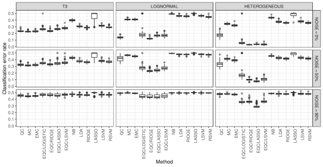
Figure 2: Low dimensional scenario test error rates, $n=200,p=50$.

In the high-dimensional case in Figure 3, the conclusions are broadly similar to the low-dimensional case in Figure 2 but with two notable differences. First, QC is much worse than the EQC/RIDGE in the LOGNORMAL scenario even when all variables are informative. Since QC lacks regularization, it becomes a victim of the accumulated noise phenomenon (Fan and Fan, 2008). Second, EQC/LASSO is much worse than EQC/RIDGE and EQC/LSVM with the low (0%) and medium (50%) level of noises since the assumption of sparse predictors made by LASSO (Hastie et al., 2009, Section 16.2.2; James et al., 2013, Section 6.2.2.3) does not hold. Conversely when the noise level is 90%, EQC/LASSO becomes competitive to EQC/RIDGE and EQC/LSVM in the scenarios of T3 and LOGNORMAL, and it becomes dominant in the HETEROGENEOUS scenario.

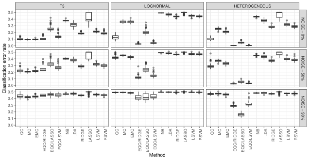
Figure 3: High dimensional scenario test error rates, $n=100,p=200$. EQC/LOGISTIC is not available in the high dimensional scenario.

Figure 4 shows that the difference in classifier performance between the independent case and the dependent case is negligible in the skewed scenarios LOGNORMAL and HETEROGENEOUS. In the T3 scenario, The performance of LDA is best and is greatly improved over the case with independent variables. This improvement is not surprising since the correlations induce heterogeneous weights on variables for the LDA (Hastie et al., 2009, Equation 4.9).

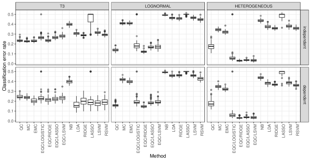
Figure 4: Comparison of test error rates with independent and correlated input variables in the low dimensional scenario, $n=200,p=50$.

4.3 Comparing EQC/RIDGE with QC for fixed ${\theta}$

Figure 5 shows the mean test rate of QC and EQC/RIDGE trained on a sample of size $n=100$ and evaluated over a grid for $\theta\in(0,1)$, where 200 simulations for $10^{4}$ test samples for each parameter setting and grid point were used. The confidence limits are too narrow to show. Looking along the first row of panels corresponding to the T3 case, the performance of EQC/RIDGE and QC is about the same for all $\theta$. Since $\theta=0.5$ corresponds to the Bayes optimal median centroid (Hall et al., 2009), both QC and EQC/RIDGE provide optimal performance in the T3 case when $\theta=0.5$. For the LOGNORMAL and HETEROGENOUS scenarios EQC/RIDGE outperforms QC. This figure demonstrates that the estimation of a suitable $\theta$ is important in achieving a low test error rate.

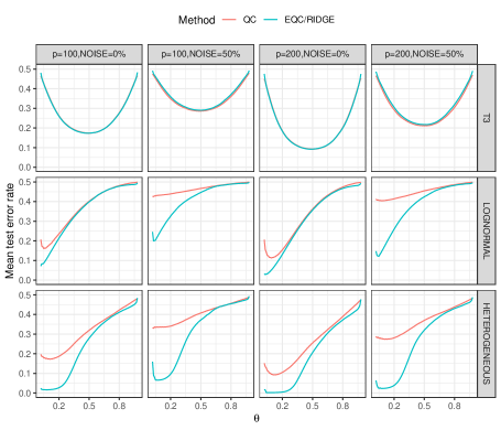
Figure 5: Mean test error rates of the QC and the EQC/RIDGE against $\theta$ for fixed $n=100$, the three distributional scenarios, the number of variables $p=100,200$ and ${\rm NOISE}=0\%,50\%$.

5 Reuters-21578 text categorization

5.1 Binary classification

As in Hall et al. (2009) we used a subset of the Reuters-21578 text categorization test collection (Lewis, 1997; Sebastiani, 2002) to demonstrate the usefulness of EQC and its improved performance over MC and QC. The improved performance may be expected since this data set is high-dimensional, sparse and the variables are highly skewed.

The subset contains two topics, “acq” and “crude”, which can be found from the R package tm (Feinerer and Hornik, 2017). The subset has 70 observations (documents), where $n_{1}=50$ are of the topic “acq” and $n_{2}=20$ are of the topic “crude”. The raw data set was preprocessed to first remove digits, punctuation marks, extra white spaces, then convert to lower case, and remove stop words and reduce to their stem. It ended up with a $70\times 1517$ document-term matrix, where a row represents a document and a column represents a term, recording the frequency of a term. A summary of the processed data set is shown in Table 1.

The performance of a classifier was assessed by the mean classification error rate estimated by 5 repetitions of 10-fold cross-validations with each fold containing $5$ documents of the topic “acq” and $2$ documents of the topic “crude”.

Since the performances of some classifiers such as the naive Bayes classifier and the LDA could be much improved by using external feature selection strategies, three external strategies for variable selection were investigated. The first strategy was to use a subset of the data by removing low frequency terms that appear in only one document, denoted by removeLowFreq. This produced a $70\times 766$ document-term matrix. The second and third strategies used Fisher’s exact test to select $L=50$ or $L=1000$ terms with the smallest p-values within each fold of the cross-validation.

Table 1: Summary of the Reuters-21578 subset.

#Classes	#Samples	#Samples(acq)	#Samples(crude)	#Features
2 (acq vs crude)	70	50	20	1517

Table 2 shows the estimated error rates and their estimated standard errors for each classifier. The second column indicates the situation where no external feature selection was used. The four EQC methods, including the EMC, performed the best even without any external feature selections, followed by the QC and the MC. It was found that most of the quantile-difference transformed variables were constants, which can be removed. This sparsity may explain the improved performance of the EQC family.

Table 2: Mean classification error rates, and their standard errors in parentheses, from 5 repetitions of 10-fold cross-validations for the Reuters-21578 subset.

Method	Classification Error Rates
	Overall	RemoveLowFreq	$L=50$	$L=1000$
QC	0.069(0.013)	0.06(0.012)	0.049(0.01)	0.063(0.012)
MC	0.06(0.012)	0.063(0.014)	0.054(0.012)	0.063(0.014)
EMC	0.034(0.01)	–	–	–
EQC/RIDGE	0.034(0.01)	–	–	–
EQC/LASSO	0.037(0.011)	–	–	–
EQC/LSVM	0.034(0.01)	–	–	–
NB	0.714(0)	0.714(0)	0.117(0.015)	0.134(0.015)
LDA	0.191(0.014)	0.18(0.019)	0.086(0.014)	0.183(0.014)
RIDGE	0.203(0.012)	0.186(0.012)	0.097(0.013)	0.203(0.012)
LASSO	0.051(0.013)	0.049(0.013)	0.066(0.014)	0.049(0.013)
LSVM	0.109(0.013)	0.1(0.013)	0.091(0.014)	0.1(0.013)
RSVM	0.217(0.012)	0.203(0.016)	0.097(0.014)	0.191(0.018)

5.2 Multiclass classification

To see how the EQC performs on the multiclass problem, a larger subset of Reuters-21578, denoted by R8 (Cardoso-Cachopo, 2007) was tried. This data set contains a training set and a test set that were obtained by applying the modApte train/test split on the raw data (Lewis, 1997). This resulted in retaining 8 classes with the highest number of positive training examples. In order to classify those 8 classes, the same preprocessing procedure as in Section 5.1 on the R8 data set was applied. The terms were preprocessed to first remove digits, punctuation marks, extra white spaces, then convert to lower case, and remove stop words and reduce to their stem. Terms that appeared in less than $0.5\%$ of documents were also removed, resulting in a $5485\times 1367$ document-term matrix for training and a $2189\times 1367$ document-term matrix for testing. The number of samples for each class is summarized in Table 3.

Classifiers in the binary case were used but with the ridge logistic regression and the LASSO logistic regression extended to the multinomial regressions, and SVM extended to multi-class SVM by the one-against-one method (Hastie et al., 2009). Table 4 shows the mean test error and the sensitivities of different classes. The EQC still outperformed the other methods on the larger subset while the EMC, the QC and the MC performed poorly this time. With a much larger sample size, the LSVM and the ridge multinomial regression were competitive with EQC.

Table 3: Summary of the Reuters-21578 subset R8 with 1367 features.

Class	#Samples
	train	test
acq	1596	696
crude	253	121
earn	2840	1083
grain	41	10
interest	190	81
money-fx	206	87
ship	108	36
trade	251	75
Total	5485	2189

Table 4: Test error rate and sensitivities for each multiclass classifier on the Reuters-21578 subset R8.

Method	Test Error	Sensitivities
		acq	crude	earn	grain	interest	money-fx	ship	trade
QC	0.144	0.963	0.745	0.857	0.333	0.763	0.663	0.481	0.757
MC	0.392	0.820	0.899	0.864	0.000	0.102	0.000	0.059	0.000
EMC	0.309	0.750	0.925	0.875	1.000	0.700	0.316	0.091	0.908
EQC	0.044	0.956	0.964	0.985	0.692	0.865	0.805	0.757	0.910
NB	0.994	0.000	0.000	0.000	0.005	1.000	1.000	0.000	1.000
LDA	0.109	0.896	0.883	0.906	1.000	0.732	0.709	0.759	0.906
RIDGE	0.060	0.934	0.944	0.956	0.833	0.946	0.839	0.923	0.850
LASSO	0.168	0.908	0.932	0.780	0.000	0.955	1.000	1.000	1.000
LSVM	0.083	0.960	0.847	0.938	0.667	0.855	0.778	0.641	0.747
RSVM	0.131	0.739	0.951	0.975	1.000	1.000	0.775	0.900	0.889

6 Discussion and conclusion

The aim of the ensemble quantile classifier is to derive a regularized weighted quantile-based classifier that can best retain the advantage of QC on skewed inputs and overcome the limitation of the QC with high-dimensional data that includes noisy inputs. The improvement using EQC has been demonstrated in simulation experiments as well as with an application to text categorization.

We implemented the EQC methods in Lai and McLeod (2018), where a vignette is available for reproducing the simulations and the Reuters text categorization application in the paper.

Appendix

Appendix A Relationship to asymmetric Laplace distribution

A random variable $x$ is said to follow the asymmetric Laplace distribution, denoted as $x\sim\textsf{AL}(m,\kappa,\lambda)$, if its probability density function has the form,

$$f(x)=\frac{\lambda}{\kappa+1/\kappa}\begin{cases}e^{\frac{\lambda}{k}(x-m)},&\text{if }x<m\\ e^{-\lambda k(x-m)},&\text{if }x\geqslant m\end{cases},$$ (13)

where $m\in\mathbb{R}$, $\lambda>0$ and $\kappa>0$ respectively are the location, the scale and the skewness parameters.

Let $\pi_{1}$ and $\pi_{2}$ be the prior probabilities of $P_{1}$ and $P_{2}$. If $P_{1}$ and $P_{2}$ consist of independent asymmetric Laplace distribution with parameters $(\bm{m_{1}},\bm{\kappa},\bm{\lambda})$ and $(\bm{m_{2}},\bm{\kappa},\bm{\lambda})$, then the Bayes decision boundary becomes $\{\,{\bm{x}}:{s_{AL}(\bm{x})=0}\,\}$ with,

$$s_{AL}(\bm{x})=\log(\pi_{2}/\pi_{1})+\sum_{j=1}^{p}\lambda_{j}(\kappa_{j}+\kappa_{j}^{-1})S_{al}(x_{j},m_{1j},m_{2j},\kappa_{j},\lambda_{j}),$$ (14)

where for $m_{1}<m_{2}$,

$$S_{al}(x,m_{1},m_{2},\kappa,\lambda)=\begin{cases}-\frac{1}{\kappa^{2}+1}(m_{2}-m_{1}),&\text{if}\ x<m_{1}\\ x-\frac{\kappa^{2}}{\kappa^{2}+1}m_{1}-\frac{1}{\kappa^{2}+1}m_{2},&\text{if}\ m_{1}\leqslant x<m_{2}\\ \frac{\kappa^{2}}{\kappa^{2}+1}(m_{2}-m_{1}),&\text{if}\ x\geqslant m_{2}\end{cases}.$$

Since $m$ is also the $[\kappa^{2}/(1+\kappa^{2})]$-quantile of an asymmetric Laplace distribution, if we let $\theta_{j}=\kappa_{j}^{2}/(1+\kappa_{j}^{2})$, Equation 14 will become the $\mathsf{C}\bigl{(}\operatorname{Q}_{\bm{\theta}}(\bm{x})\mid\beta_{0},\bm{\beta}\bigr{)}$ of EQC in Equation 6 with $\beta_{0}=\log(\pi_{2}/\pi_{1})$ and $\beta_{j}=\lambda_{j}\sqrt{[\theta_{j}(1-\theta_{j})]^{-1}}$ for $j=1,\dotsc,p$. If $x_{j}$’s are rescaled by its standard deviation $\sqrt{1+\kappa^{4}}/(\lambda\kappa)$ first, then the $\bm{\beta}$ will become

$$\beta_{j}=\frac{\sqrt{2}}{\theta_{j}(1-\theta_{j})}\sqrt{(\theta_{j}-\frac{1}{2})^{2}+\frac{1}{4}},\text{ for }j=1,\dotsc,p.$$ (15)

Therefore, we can see that the decision boundary given by the EQC is the Bayes decision boundary in this special case while QC cannot be if $\bm{\kappa}$ is not homogeneous.

Appendix B Maximum likelihood estimation of multiclass EQC

In this section, we formulate the log-likelihood function of for the multiclass EQC in a matrix form as well as its gradient vector and Hessian function. This is useful for further investigation of theoretical properties and the ease of computation. At the end, we will show that the Hessian matrix is semi-negative-definite so the log-likelihood function has a single, unique maximum.

Without loss of generality, we let $\beta_{0,k}=0$ for all $k=1,\dotsc,K-1$ and disregard them. Define $\bm{1}_{K}=(1)_{1\times K}$, $\bm{1}_{n}=(1)_{1\times n}$, $\bm{Y}=(y_{k,i})_{K\times n}$, where $y_{k,i}=1$ if $y_{i}=k$ and $0$ otherwise. We also define,

$$\bm{Q}_{i}=\begin{pmatrix}-\operatorname{Q}_{\bm{\theta}}^{(1,K)}(\bm{x}_{i})\\ \vdots\\ -\operatorname{Q}_{\bm{\theta}}^{(K,K)}(\bm{x}_{i})\end{pmatrix},\text{ for }i=1,\dotsc,n,$$

$$\bm{Q}=\begin{pmatrix}\bm{Q}_{1}\\ \vdots\\ \bm{Q}_{n}\end{pmatrix},$$

$$\bm{\beta}=(\beta_{1},\dotsc,\beta_{p})^{{\mathchoice{\raisebox{0.0pt}{$\displaystyle\intercal$}}{\raisebox{0.0pt}{$\textstyle\intercal$}}{\raisebox{0.0pt}{$\scriptstyle\intercal$}}{\raisebox{0.0pt}{$\scriptscriptstyle\intercal$}}}},$$

and

$$\bm{C} =\Bigl{(}C_{1}(\bm{\beta}),\dotsc,C_{n}(\bm{\beta})\Bigr{)}^{{\mathchoice{\raisebox{0.0pt}{$\displaystyle\intercal$}}{\raisebox{0.0pt}{$\textstyle\intercal$}}{\raisebox{0.0pt}{$\scriptstyle\intercal$}}{\raisebox{0.0pt}{$\scriptscriptstyle\intercal$}}}}$$

$$=\begin{pmatrix}\bm{1}_{K}\exp[\bm{Q}_{1}\bm{\beta}]\\ \vdots\\ \bm{1}_{K}\exp[\bm{Q}_{n}\bm{\beta}]\end{pmatrix}$$

$$=\bm{B}_{1}\exp[\bm{Q}\bm{\beta}],$$

where $\exp[\cdot]$ is the entrywise exponential operation and $\bm{B}_{1}=\operatorname{diag}_{n}(\bm{1}_{K},\dotsc,\bm{1}_{K})$ is a block diagonal matrix consisting of $n$ repetitions of $\bm{1}_{K}$.

Then the log-likelihood function of EQC given $\bm{\theta}$ can be expressed,

$$\ell(\bm{\beta}) =\operatorname{vec}[\bm{Y}]^{{\mathchoice{\raisebox{0.0pt}{$\displaystyle\intercal$}}{\raisebox{0.0pt}{$\textstyle\intercal$}}{\raisebox{0.0pt}{$\scriptstyle\intercal$}}{\raisebox{0.0pt}{$\scriptscriptstyle\intercal$}}}}\bm{Q}\bm{\beta}-\bm{1}_{n}\log[\bm{C}]$$

$$=\operatorname{vec}[\bm{Y}]^{{\mathchoice{\raisebox{0.0pt}{$\displaystyle\intercal$}}{\raisebox{0.0pt}{$\textstyle\intercal$}}{\raisebox{0.0pt}{$\scriptstyle\intercal$}}{\raisebox{0.0pt}{$\scriptscriptstyle\intercal$}}}}\bm{Q}\bm{\beta}-\bm{1}_{n}\log\Bigl{[}B_{1}\exp[\bm{Q}\bm{\beta}]\Bigr{]},$$ (16)

where $\log[\cdot]$ is the entrywise natural logarithm operation and $\operatorname{vec}[\cdot]$ is a matrix vectorization operation which creates a column vector by appending all columns of the matrix.

The gradient vector can be expressed,

$$\nabla\ell(\bm{\beta})=\operatorname{vec}[\bm{Y}]^{{\mathchoice{\raisebox{0.0pt}{$\displaystyle\intercal$}}{\raisebox{0.0pt}{$\textstyle\intercal$}}{\raisebox{0.0pt}{$\scriptstyle\intercal$}}{\raisebox{0.0pt}{$\scriptscriptstyle\intercal$}}}}\bm{Q}-\bm{1}_{n}\Bigl{[}\bm{A}\oslash\bm{E}_{2}\Bigr{]},$$ (17)

where

$$\bm{A}=\bm{B}_{1}\,\bm{U},$$

$$\bm{U}=\bm{Q}\odot\bm{E}_{1},$$

$\odot$ stands for the entrywise multiplication or the Hadamard product and $\oslash$ stands for the entrywise division, $\bm{E}_{1}$ is an $nK\times p$ matrix with $p$ repeated columns of $\exp[\bm{Q}\bm{\beta}]$, which is,

$$\bm{E}_{1}=\underbrace{\begin{pmatrix}\exp[\bm{Q}\bm{\beta}]&\dotsc&\exp[\bm{Q}\bm{\beta}]\end{pmatrix}}_{p\text{ repeated columns}},$$

and $\bm{E}_{2}$ is an $n\times p$ matrix with $p$ repeated columns of $\bm{C}=\bm{B}_{1}\exp[\bm{Q}\bm{\beta}]$, which is,

$$\bm{E}_{2}=\underbrace{\begin{pmatrix}\bm{C}&\dotsc&\bm{C}\end{pmatrix}}_{p\text{ repeated columns}}.$$

In particular, the $j$-th element of $\nabla\ell(\bm{\beta})$ is, for $j=1,\dotsc,p$,

$$\nabla_{j}\ell(\bm{\beta})=\operatorname{vec}[\bm{Y}]^{{\mathchoice{\raisebox{0.0pt}{$\displaystyle\intercal$}}{\raisebox{0.0pt}{$\textstyle\intercal$}}{\raisebox{0.0pt}{$\scriptstyle\intercal$}}{\raisebox{0.0pt}{$\scriptscriptstyle\intercal$}}}}\bm{Q}\bm{e}_{j}-\bm{1}_{n}\bigl{[}\bm{A}_{j}\oslash C\bigr{]},$$

where

$$\bm{A}_{j}=\bm{A}\bm{e}_{j}=\bm{B}_{1}\,\bigl{[}\bm{Q}\bm{e}_{j}\odot\exp(\bm{Q}\bm{\beta})\bigr{]},$$

$\bm{e}_{j}$ is a unit column vector of length $p$ where the $j$-th element is $1$ and the other elements are $0$’s.

The $j$-th row of the Hessian matrix can be expressed as, for $j=1,\dotsc,p$,

$$\nabla\bigl{(}\nabla_{j}\ell(\bm{\beta})\bigr{)}=\bm{F}_{j}\bm{A}-[\bm{1}_{n}\oslash\bm{C}^{\mathchoice{\raisebox{0.0pt}{$\displaystyle\intercal$}}{\raisebox{0.0pt}{$\textstyle\intercal$}}{\raisebox{0.0pt}{$\scriptstyle\intercal$}}{\raisebox{0.0pt}{$\scriptscriptstyle\intercal$}}}]\,\bm{B}_{1}\bm{G}_{j},$$ (18)

where

$$\bm{F}_{j}=\bigl{[}\bm{A}_{j}\oslash[\bm{C}\odot\bm{C}]\bigr{]}^{{\mathchoice{\raisebox{0.0pt}{$\displaystyle\intercal$}}{\raisebox{0.0pt}{$\textstyle\intercal$}}{\raisebox{0.0pt}{$\scriptstyle\intercal$}}{\raisebox{0.0pt}{$\scriptscriptstyle\intercal$}}}},$$

and

$$\bm{G}_{j}=\bm{U}\odot\bm{E}_{3,j},$$

and

$$\bm{E}_{3,j}=\underbrace{\begin{pmatrix}\bm{Q}\bm{e}_{j}&\dotsc&\bm{Q}\bm{e}_{j}\end{pmatrix}}_{p\text{ repeated columns}}.$$

Then the Hessian matrix can be expressed,

$$\nabla^{2}\ell(\bm{\beta})=\begin{pmatrix}\bm{F}_{1}\\ \vdots\\ \bm{F}_{p}\end{pmatrix}\bm{A}-\bm{B}_{2}\begin{pmatrix}\bm{G}_{1}\\ \vdots\\ \bm{G}_{p}\end{pmatrix}$$ (19)

where $\bm{B}_{2}=\operatorname{diag}_{p}\bigl{(}[\bm{1}_{n}\oslash\bm{C}^{\mathchoice{\raisebox{0.0pt}{$\displaystyle\intercal$}}{\raisebox{0.0pt}{$\textstyle\intercal$}}{\raisebox{0.0pt}{$\scriptstyle\intercal$}}{\raisebox{0.0pt}{$\scriptscriptstyle\intercal$}}}]\,\bm{B}_{1},\dotsc,[\bm{1}_{n}\oslash\bm{C}^{\mathchoice{\raisebox{0.0pt}{$\displaystyle\intercal$}}{\raisebox{0.0pt}{$\textstyle\intercal$}}{\raisebox{0.0pt}{$\scriptstyle\intercal$}}{\raisebox{0.0pt}{$\scriptscriptstyle\intercal$}}}]\,\bm{B}_{1}\bigl{)}$ is a block diagonal matrix consists of $p$ repetitions of $[\bm{1}_{n}\oslash\bm{C}^{\mathchoice{\raisebox{0.0pt}{$\displaystyle\intercal$}}{\raisebox{0.0pt}{$\textstyle\intercal$}}{\raisebox{0.0pt}{$\scriptstyle\intercal$}}{\raisebox{0.0pt}{$\scriptscriptstyle\intercal$}}}]\,\bm{B}_{1}$.

If we let $\bm{W}_{1}=\operatorname{diag}_{nK}\bigl{(}\exp(\bm{Q}\bm{\beta})\bigr{)}$, $\bm{W}_{2}=\operatorname{diag}_{n}(\bm{1}_{n}\oslash\bm{C}^{\mathchoice{\raisebox{0.0pt}{$\displaystyle\intercal$}}{\raisebox{0.0pt}{$\textstyle\intercal$}}{\raisebox{0.0pt}{$\scriptstyle\intercal$}}{\raisebox{0.0pt}{$\scriptscriptstyle\intercal$}}})$, and

$$\bm{W}_{3}=\operatorname{diag}_{nK}(\underbrace{\frac{1}{C_{1}(\bm{\beta)}},\dotsc,\frac{1}{C_{1}(\bm{\beta)}}}_{K},\dotsc,\underbrace{\frac{1}{C_{n}(\bm{\beta)}},\dotsc,\frac{1}{C_{n}(\bm{\beta)}}}_{K}),$$

then $\bm{A}$ can be expressed,

$$\bm{A}=\bm{B}_{1}\bm{W}_{1}\bm{Q},$$

and Equation 17 and Equation 19 can also be expressed,

$$\nabla\ell(\bm{\beta})=\operatorname{vec}[\bm{Y}]^{{\mathchoice{\raisebox{0.0pt}{$\displaystyle\intercal$}}{\raisebox{0.0pt}{$\textstyle\intercal$}}{\raisebox{0.0pt}{$\scriptstyle\intercal$}}{\raisebox{0.0pt}{$\scriptscriptstyle\intercal$}}}}\bm{Q}-\bm{1}_{n}\bm{W}_{2}\bm{A},$$

and

$$\nabla^{2}\ell(\bm{\beta}) =\bm{A}^{\mathchoice{\raisebox{0.0pt}{$\displaystyle\intercal$}}{\raisebox{0.0pt}{$\textstyle\intercal$}}{\raisebox{0.0pt}{$\scriptstyle\intercal$}}{\raisebox{0.0pt}{$\scriptscriptstyle\intercal$}}}\bm{W}_{2}^{2}\bm{A}-\bm{Q}^{\mathchoice{\raisebox{0.0pt}{$\displaystyle\intercal$}}{\raisebox{0.0pt}{$\textstyle\intercal$}}{\raisebox{0.0pt}{$\scriptstyle\intercal$}}{\raisebox{0.0pt}{$\scriptscriptstyle\intercal$}}}\bm{W}_{3}\bm{W}_{1}\bm{Q}$$

$$=\bm{Q}^{\mathchoice{\raisebox{0.0pt}{$\displaystyle\intercal$}}{\raisebox{0.0pt}{$\textstyle\intercal$}}{\raisebox{0.0pt}{$\scriptstyle\intercal$}}{\raisebox{0.0pt}{$\scriptscriptstyle\intercal$}}}\bm{W}_{1}^{\mathchoice{\raisebox{0.0pt}{$\displaystyle\intercal$}}{\raisebox{0.0pt}{$\textstyle\intercal$}}{\raisebox{0.0pt}{$\scriptstyle\intercal$}}{\raisebox{0.0pt}{$\scriptscriptstyle\intercal$}}}\bigl{[}\bm{B}_{1}^{\mathchoice{\raisebox{0.0pt}{$\displaystyle\intercal$}}{\raisebox{0.0pt}{$\textstyle\intercal$}}{\raisebox{0.0pt}{$\scriptstyle\intercal$}}{\raisebox{0.0pt}{$\scriptscriptstyle\intercal$}}}\bm{W}_{2}^{2}\bm{B}_{1}-\bm{W}_{1}^{-1}\bm{W}_{3}\bigr{]}\bm{W}_{1}\bm{Q}.$$

In particular, $\bigl{[}\bm{B}_{1}^{\mathchoice{\raisebox{0.0pt}{$\displaystyle\intercal$}}{\raisebox{0.0pt}{$\textstyle\intercal$}}{\raisebox{0.0pt}{$\scriptstyle\intercal$}}{\raisebox{0.0pt}{$\scriptscriptstyle\intercal$}}}\bm{W}_{2}^{2}\bm{B}_{1}-\bm{W}_{1}^{-1}\bm{W}_{3}\bigr{]}$ is a negative semi-definite diagonal matrix as its eigenvalues are all non-positive. We can then conclude that the Hessian of $\ell(\bm{\beta})$ is a negative semi-definite matrix and so is its L2 regularized version.

Appendix C Proof of the consistency of estimating EQC

Without loss of generality, we set $\beta_{0}=0$ and disregard it in the following discussions.

Proof of 1.

For abbreviation, denote $\bm{\eta}=(\bm{\theta},\bm{\beta})$. From the continuity implied by 3 later on, we only need to show the following converges to zero,

$$\lvert\Psi(\tilde{\bm{\eta}})-\Psi(\hat{\bm{\eta}}_{n})\rvert\leqslant\lvert\Psi(\tilde{\bm{\eta}})-\Psi_{n}(\tilde{\bm{\eta}})\rvert+\lvert\Psi_{n}(\tilde{\bm{\eta}})-\Psi_{n}(\hat{\bm{\eta}}_{n})\rvert+\lvert\Psi_{n}(\hat{\bm{\eta}_{n}})-\Psi(\hat{\bm{\eta}}_{n})\rvert.$$ (20)

By 4 later on, under Assumptions 1 and 2, $\forall\epsilon>0$,

$$\lim_{n\rightarrow\infty}\mathbb{P}\{\sup_{\bm{\eta}\in\mathbb{S}}\lvert\Psi_{n}(\bm{\eta})-\Psi(\bm{\eta})\rvert>\epsilon\}=0,$$ (21)

where $\mathbb{S}\subset({0},{1})^{p}\times\mathbb{R}^{p}$.

So Equation 21 forces the first and the third term of the right hand side of Equation 20 to converge to 0 in probability.

Consider the second term now. By definitions of $\tilde{\bm{\eta}}$ and $\hat{\bm{\eta}}$,

$$\Psi(\tilde{\bm{\eta}})\geqslant\Psi(\hat{\bm{\eta}}_{n}),\ \Psi_{n}(\tilde{\bm{\eta}})\leqslant\Psi_{n}(\hat{\bm{\eta}}_{n}).$$

So

$$\lvert\Psi_{n}(\tilde{\bm{\eta}})-\Psi_{n}(\hat{\bm{\eta}}_{n})\rvert= \Psi_{n}(\hat{\bm{\eta}}_{n})-\Psi_{n}(\tilde{\bm{\eta}})$$

$$= [\Psi_{n}(\hat{\bm{\eta}}_{n})-\Psi(\hat{\bm{\eta}}_{n})]+[\Psi(\hat{\bm{\eta}}_{n})-\Psi_{n}(\tilde{\bm{\eta}})]$$

$$\leqslant [\Psi_{n}(\hat{\bm{\eta}}_{n})-\Psi(\hat{\bm{\eta}}_{n})]+[\Psi(\tilde{\bm{\eta}})-\Psi_{n}(\tilde{\bm{\eta}})].$$

Using Equation 21 again, then both $\lvert\Psi_{n}(\hat{\bm{\eta}}_{n})-\Psi(\hat{\bm{\eta}}_{n})\rvert$ and $\lvert\Psi(\tilde{\bm{\eta}})-\Psi_{n}(\tilde{\bm{\eta}})\rvert$ will converge to zero in probability. This makes $\lvert\Psi_{n}(\tilde{\bm{\eta}})-\Psi_{n}(\hat{\bm{\eta}}_{n})\rvert$ converge to zero in probability. Therefore, Equation 20 converges to zero in probability. That is,

$$\lim_{n\rightarrow\infty}\mathbb{P}\{\lvert\Psi(\tilde{\bm{\eta}})-\Psi(\hat{\bm{\eta}}_{n})\rvert>\epsilon\}=0.$$

∎

Proof of 2.

For abbreviation, denote $\bm{\eta}=(\bm{\theta},\bm{\beta})$. We will investigate

$$\lvert\Psi(\tilde{\bm{\eta}})-\Psi_{n}(\hat{\bm{\eta}}_{n})\rvert\leqslant\lvert\Psi(\tilde{\bm{\eta}})-\Psi(\hat{\bm{\eta}}_{n})\rvert+\lvert\Psi(\hat{\bm{\eta}}_{n})-\Psi_{n}(\hat{\bm{\eta}}_{n})\rvert.$$ (22)

By 1, the first term of the right hand side above converges to zero in probability. By 4, the second term of the right hand side above also converges to zero in probability. Therefore, $\lvert\Psi(\tilde{\bm{\eta}})-\Psi_{n}(\hat{\bm{\eta}}_{n})\rvert$ converges to zero in probability and we complete the proof. ∎

Lemma 3.

Under the assumption that $\theta_{1}\leqslant\theta_{2}$ and $q_{1}\leqslant q_{2}$, or $\theta_{1}\geqslant\theta_{2}$ and $q_{1}\geqslant q_{2}$, the following inequality holds,

$$\lvert\rho_{\theta_{1}}(x_{j}-q_{1}(\theta_{1}))-\rho_{\theta_{2}}(x_{j}-q_{2}(\theta_{2}))\rvert\leqslant\lvert x_{j}\rvert\lvert\theta_{2}-\theta_{1}\rvert+4\lvert q_{1}-q_{2}\rvert,\ j=1,\dotsc,p,$$

which further implies the continuity of $\mathsf{C}(\operatorname{Q}_{\bm{\theta}}(\bm{x})\mid\bm{\beta})$ under Assumptions 1 and 2, and hence the continuity of $\Psi(\bm{\theta},\bm{\beta})$.

Proof.

The inequality follows directly from the Lemma 3 in the supplementary material of Hennig and Viroli (2016a).

It implies that the quantile-based transformation $\operatorname{Q}_{\bm{\theta}}(\bm{x})$ is a continuous function of $\bm{\theta}$. Furthermore, since empirical quantiles are strongly consistent, $\bm{\beta}$ is bounded and $\mathsf{C}(\bm{z}\mid\bm{\beta})$ is required to be differentiable with respect to $\bm{z}$ and $\bm{\beta}$ by Assumption 2, then $\mathsf{C}(\operatorname{Q}_{\bm{\theta}}(\bm{x})\mid\bm{\beta})$ is bounded and a continuous function of $\bm{\theta}$ and $\bm{\beta}$. So the dominated convergence theorem still makes the integrals of the differentiable transformation of $\mathsf{C}(\operatorname{Q}_{\bm{\theta}}(\bm{x})\mid\bm{\beta})$ continuous with respect to $\bm{\theta}$ and $\bm{\beta}$.

∎

Lemma 4.

Under Assumptions 1 and 2, $\forall\epsilon>0$,

$$\lim_{n\rightarrow\infty}\mathbb{P}\{\sup_{\bm{\eta}\in\mathbb{S}}\lvert\Psi_{n}(\bm{\eta})-\Psi(\bm{\eta})\rvert>\epsilon\}=0,$$

where $\bm{\eta}=(\bm{\theta},\bm{\beta})$ and $\mathbb{S}\subset({0},{1})^{p}\times\mathbb{R}^{p}$,

Proof.

Assuming that the conclusion does not hold, since $\bm{\eta}$ is bounded according to Assumption 2, then $\exists\epsilon>0$, $\delta>0$, there is a convergent subsequence $\mathopen{}\mathclose{{}\left\{\cramped{\bm{\eta}^{*}_{m}}}\right\}_{{m}=1}^{\infty}$ with limit $\bm{\eta}^{*}=\lim_{m\rightarrow\infty}\bm{\eta}^{*}_{m}$ such that for $m=1,\dotsc$,

$$\mathbb{P}\{\lvert\Psi_{m}(\bm{\eta}_{m}^{*})-\Psi(\bm{\eta}_{m}^{*})\rvert>\epsilon\}\geqslant\delta.$$ (23)

Consider

$$\lvert\Psi_{m}(\bm{\eta}^{*}_{m})-\Psi(\bm{\eta}^{*}_{m})\rvert\leqslant\lvert\Psi_{m}(\bm{\eta}^{*}_{m})-\Psi_{m}(\bm{\eta}^{*})\rvert+\lvert\Psi_{m}(\bm{\eta}^{*})-\Psi(\bm{\eta}^{*})\rvert+\lvert\Psi(\bm{\eta}^{*})-\Psi(\bm{\eta}^{*}_{m})\rvert.$$ (24)

Firstly, continuity of $\Psi(\bm{\eta})$ implies that the third term of the right side of Equation 24 converges to $0$ as $m\rightarrow\infty$.

Consider the second term, we define a new $\Psi_{n}$ with the true quantiles below, where the empirical decision rule $\mathsf{C}(\hat{\operatorname{Q}}_{\bm{\theta}}(\bm{x})\mid\bm{\beta})$ in Equation 12 is replaced by the population decision rule $\mathsf{C}(\operatorname{Q}_{\bm{\theta}}(\bm{x})\mid\bm{\beta})$.

$$\Psi_{m}^{*}(\bm{\eta})=-\frac{1}{m}\sum_{i=1}^{m}\Bigl{\{}(y_{i}-1)\mathsf{C}\bigl{(}\operatorname{Q}_{\bm{\theta}}(\bm{x}_{i})\mid\bm{\beta}\bigr{)}-\log(1+e^{\mathsf{C}(\operatorname{Q}_{\bm{\theta}}(\bm{x}_{i})\mid\bm{\beta})})\Bigr{\}}.$$

Consider

$$\lvert\Psi_{m}(\bm{\eta}^{*})-\Psi(\bm{\eta}^{*})\rvert\leqslant\lvert\Psi_{m}(\bm{\eta}^{*})-\Psi^{*}_{m}(\bm{\eta}^{*})\rvert+\lvert\Psi^{*}_{m}(\bm{\eta}^{*})-\Psi(\bm{\eta}^{*})\rvert.$$

Following the strong law of large numbers, $\lvert\Psi^{*}_{m}(\bm{\eta}^{*})-\Psi(\bm{\eta}^{*})\rvert\overset{\text{a.s.}}{\rightarrow}0$ as $m\rightarrow\infty$.

Since empirical quantiles are strongly consistent and $\mathsf{C}(\bm{z}\mid\bm{\beta})$ is required to be differentiable with respect to $\bm{z}$ and $\bm{\beta}$ by Assumption 2, then $\lvert\mathsf{C}\bigl{(}\hat{\operatorname{Q}}_{\bm{\theta}^{*}}(\bm{x})\mid\bm{\beta}^{*}\bigr{)}-\mathsf{C}\bigl{(}\operatorname{Q}_{\bm{\theta}^{*}}(\bm{x})\mid\bm{\beta}^{*}\bigr{)}\rvert\overset{\text{a.s.}}{\rightarrow}0$ as $m\rightarrow\infty$, and hence $\lvert\Psi_{m}(\bm{\eta}^{*})-\Psi^{*}_{m}(\bm{\eta}^{*})\rvert\overset{\text{a.s.}}{\rightarrow}0$ as $m\rightarrow\infty$.

Now consider the first term of the right hand side of Equation 24. Firstly, for $j=1,\dotsc,p$,

$$\lvert\hat{q}_{k,j,m}(\theta_{j,m}^{*})-\hat{q}_{k,j,m}(\theta_{j}^{*})\rvert\leqslant\lvert\hat{q}_{k,j,m}(\theta_{j,m}^{*})-q_{k,j}(\theta_{j,m}^{*})\rvert+\lvert q_{k,j}(\theta_{j,m}^{*})-\hat{q}_{k,j}(\theta_{j}^{*})\rvert+\lvert q_{k,j}(\theta_{j}^{*})-\hat{q}_{k,j,m}(\theta_{j}^{*})\rvert.$$

From Theorem 3 in Mason (1982) and Assumption 1, all terms on the right side of the above inequality converge to zero almost surely, and hence $\lvert\hat{q}_{k,j,m}(\theta_{j,m}^{*})-\hat{q}_{k,j,m}(\theta_{j}^{*})\rvert\overset{\text{a.s.}}{\rightarrow}0$ as $m\rightarrow\infty$ for $j=1,\dotsc,p$. Thus $||\hat{\operatorname{Q}}_{\bm{\theta}^{*}_{m}}(\bm{x})-\hat{\operatorname{Q}}_{\bm{\theta}^{*}}(\bm{x})||\overset{\text{a.s.}}{\rightarrow}0$ as $m\rightarrow\infty$, where $||\cdot||$ represents L2 norm.

Furthermore, since $\mathsf{C}(\bm{z}\mid\bm{\beta})$ is required to be differentiable with respect to $\bm{z}$ and $\bm{\beta}$ by Assumption 2, then $\lvert\mathsf{C}\bigl{(}\hat{\operatorname{Q}}_{\bm{\theta}^{*}_{m}}(\bm{x})\mid\bm{\beta}^{*}_{m}\bigr{)}-\mathsf{C}\bigl{(}\hat{\operatorname{Q}}_{\bm{\theta}^{*}}(\bm{x})\mid\bm{\beta}\bigr{)}\rvert\overset{\text{a.s.}}{\rightarrow}0$ as $m\rightarrow\infty$. Thus the first term of the right hand side of Equation 24 converges to zero almost surely, $\lvert\Psi_{m}(\bm{\eta}_{m}^{*})-\Psi_{m}(\bm{\eta}^{*})\rvert\overset{\text{a.s.}}{\rightarrow}0$ as $m\rightarrow\infty$.

To sum up, $\lvert\Psi^{*}_{m}(\bm{\eta}_{n_{i}})-\Psi(\bm{\eta}^{*}_{m})\rvert\overset{\text{a.s.}}{\rightarrow}0$, which is contradictory to Equation 23 and hence we conclude that, under Assumptions 1 and 2, $\forall\epsilon>0$,

$$\lim_{n\rightarrow\infty}\mathbb{P}\{\sup_{\bm{\eta}\in\mathbb{S}}\lvert\Psi_{n}(\bm{\eta})-\Psi(\bm{\eta})\rvert>\epsilon\}=0,$$

where $\mathbb{S}\subset({0},{1})^{p}\times\mathbb{R}^{p}$. ∎

Appendix D Misclassification rates

In Section 4.2, we presented boxplots of the test misclassification error rates for each classifier. Their averages and standard deviations are tabulated in tables 5 to Table 10, for the T3, LOGNORMAL and HETEROGENEOUS distribution cases with independent or dependent variables.

Table 5: Simulation study: the mean test classification error rates, and their standard errors in parentheses, of each method for the independent T3 scenario. All numbers are in percentages and rounded to one digit. The third line indicates the percentage of irrelevant variables within $p$ variables.

$n=100$
	$p=50$			$p=100$			$p=200$
	$0\%$	$50\%$	$90\%$	$0\%$	$50\%$	$90\%$	$0\%$	$50\%$	$90\%$
QC	27.1(0.3)	35.9(0.4)	47.2(0.2)	18.5(0.2)	30.4(0.3)	46(0.2)	10(0.1)	22.3(0.3)	43.9(0.3)
MC	25.5(0.1)	33.9(0.2)	46(0.2)	17.6(0.1)	28.5(0.2)	44.4(0.1)	9.1(0.1)	20.8(0.1)	42.2(0.1)
EMC	26.1(0.2)	35(0.2)	46.6(0.2)	18.2(0.2)	29.7(0.2)	45.2(0.2)	9.5(0.1)	21.9(0.2)	43(0.2)
EQC/LOGISTIC	32.1(0.4)	40.3(0.4)	47.9(0.2)	24.7(0.3)	35.4(0.3)	47.6(0.2)	-	-	-
EQC/RIDGE	28.4(0.4)	37.9(0.5)	48(0.2)	19.4(0.3)	32(0.4)	47.1(0.2)	10.6(0.2)	23.9(0.4)	44.6(0.2)
EQC/LASSO	33.5(0.5)	40.2(0.4)	47.8(0.2)	28.6(0.3)	37.2(0.3)	47(0.2)	25.8(0.4)	32.7(0.4)	46(0.2)
EQC/LSVM	33.5(0.4)	40.5(0.4)	48.4(0.2)	24.5(0.3)	35.9(0.3)	47.6(0.2)	14.1(0.3)	26.8(0.3)	45.4(0.2)
NB	41.5(0.1)	43.8(0.2)	48.2(0.1)	39.8(0.1)	42.3(0.1)	47.6(0.1)	37.8(0.1)	40.5(0.1)	46.7(0.1)
LDA	35.8(0.2)	41.3(0.2)	48.2(0.2)	44.9(0.3)	47.1(0.2)	49.2(0.1)	31.4(0.3)	38.3(0.2)	47.4(0.1)
RIDGE	31(0.2)	38.4(0.2)	47.3(0.2)	25.3(0.1)	34.4(0.2)	46.3(0.1)	18.4(0.1)	28.9(0.2)	44.8(0.1)
LASSO	45.5(0.5)	47.7(0.4)	49(0.2)	44.3(0.6)	46.4(0.4)	49(0.2)	42.5(0.7)	45.5(0.5)	49.2(0.2)
LSVM	36.2(0.3)	41.9(0.2)	48.1(0.2)	29.8(0.2)	38.2(0.2)	47.3(0.1)	21.3(0.1)	32(0.2)	45.9(0.1)
RSVM	32.1(0.2)	39.2(0.2)	47.6(0.2)	26.3(0.2)	35.3(0.2)	46.6(0.1)	18.7(0.2)	29.6(0.2)	45.2(0.1)
$n=200$
	$p=50$			$p=100$			$p=200$
	$0\%$	$50\%$	$90\%$	$0\%$	$50\%$	$90\%$	$0\%$	$50\%$	$90\%$
QC	23.5(0.1)	32.6(0.2)	45.9(0.2)	15.1(0.1)	25.8(0.2)	43.7(0.2)	7.4(0.1)	17.8(0.1)	41.1(0.2)
MC	22.8(0.1)	31.6(0.1)	44.5(0.1)	14.5(0.1)	25(0.1)	42.5(0.1)	6.8(0)	17.1(0.1)	39.5(0.1)
EMC	23.2(0.1)	32.3(0.1)	45(0.1)	14.8(0.1)	25.7(0.2)	43.3(0.1)	7.3(0.1)	18.1(0.1)	40.5(0.1)
EQC/LOGISTIC	26.8(0.3)	35.1(0.2)	46.9(0.2)	20.6(0.2)	31.9(0.3)	46(0.2)	13.3(0.1)	24.7(0.2)	43.9(0.2)
EQC/RIDGE	23.7(0.2)	33.1(0.2)	46.6(0.2)	15.5(0.2)	26.5(0.2)	44.9(0.2)	7.7(0.1)	18.7(0.2)	42.2(0.3)
EQC/LASSO	26.8(0.2)	34.9(0.3)	46.3(0.2)	22.3(0.2)	30.9(0.3)	45.2(0.2)	18.8(0.2)	26.3(0.2)	43.3(0.2)
EQC/LSVM	28.1(0.2)	35.8(0.3)	47.1(0.2)	22.1(0.2)	32.6(0.3)	46.5(0.2)	11.9(0.1)	24.1(0.2)	44.1(0.2)
NB	39.8(0.1)	42.8(0.2)	47.5(0.1)	37.9(0.1)	40.5(0.1)	46.7(0.1)	35.3(0.1)	38.7(0.1)	45.6(0.1)
LDA	30.6(0.1)	37.8(0.2)	46.9(0.1)	28.5(0.2)	36.3(0.2)	46.3(0.1)	43.8(0.3)	46.7(0.3)	49(0.1)
RIDGE	28.8(0.1)	36.3(0.2)	46.4(0.1)	22.7(0.1)	31.7(0.1)	44.9(0.1)	15.7(0.1)	26(0.1)	43(0.1)
LASSO	44.9(0.6)	46.8(0.4)	48.7(0.2)	41.1(0.9)	45.8(0.5)	48.3(0.3)	32.9(1)	44.1(0.5)	47.7(0.3)
LSVM	31.6(0.1)	38.3(0.2)	47(0.1)	28.1(0.2)	37.1(0.2)	46.6(0.1)	19.6(0.1)	30.5(0.1)	45(0.1)
RSVM	29.4(0.1)	37(0.2)	46.7(0.1)	22.8(0.1)	32.2(0.1)	45.2(0.1)	15.2(0.1)	26.7(0.1)	43.7(0.1)

Table 6: Simulation study: the mean test classification error rates, and their standard errors in parentheses, of each method for the dependent T3 scenario. All numbers are in percentages and rounded to one digit. The third line indicates the percentage of irrelevant variables within $p$ variables.

$n=100$
	$p=50$			$p=100$			$p=200$
	$0\%$	$50\%$	$90\%$	$0\%$	$50\%$	$90\%$	$0\%$	$50\%$	$90\%$
QC	28.9(0.3)	36.9(0.3)	46.9(0.2)	20.8(0.2)	30.9(0.3)	45.6(0.2)	11.8(0.2)	24(0.3)	43.7(0.2)
MC	27.3(0.2)	35.1(0.2)	45.8(0.1)	19.9(0.2)	29.4(0.2)	44.2(0.1)	11(0.1)	22.5(0.1)	42.3(0.1)
EMC	25.1(0.3)	34.6(0.3)	46(0.2)	18.2(0.2)	29.1(0.2)	44.6(0.1)	10.2(0.1)	22.6(0.2)	42.9(0.1)
EQC/LOGISTIC	28.3(0.4)	38.1(0.4)	47.4(0.2)	21.5(0.3)	32.4(0.3)	47.1(0.2)	-	-	-
EQC/RIDGE	26.5(0.4)	36(0.4)	47.3(0.2)	19.4(0.3)	31(0.3)	46.5(0.2)	10.8(0.2)	24.2(0.3)	44.6(0.2)
EQC/LASSO	29.2(0.5)	37.5(0.5)	47.3(0.2)	26.2(0.3)	33.6(0.4)	46.9(0.2)	24.9(0.3)	32.3(0.4)	45.9(0.3)
EQC/LSVM	28.5(0.3)	37.6(0.4)	47.7(0.2)	20.8(0.3)	32.9(0.3)	46.9(0.2)	12(0.2)	25.4(0.3)	45.4(0.2)
NB	41.4(0.2)	43.9(0.2)	48(0.1)	39.6(0.1)	42.5(0.1)	47.6(0.1)	37.6(0.1)	40.4(0.1)	46.7(0.1)
LDA	21.7(0.5)	29.5(0.6)	44.1(0.5)	38.6(0.5)	42.4(0.4)	48.3(0.2)	31.8(0.3)	40.8(0.2)	47.9(0.1)
RIDGE	28.4(0.4)	38(0.3)	47.2(0.1)	23.3(0.3)	34.3(0.2)	46.2(0.1)	17(0.2)	29.1(0.2)	44.7(0.1)
LASSO	43.7(0.9)	46.4(0.7)	49.3(0.3)	43.6(0.7)	46.9(0.4)	49.4(0.2)	44.3(0.7)	46.1(0.5)	49.5(0.1)
LSVM	23.2(0.5)	32.6(0.5)	45.6(0.4)	21.5(0.3)	33.2(0.3)	46.2(0.2)	17.2(0.2)	29.3(0.2)	45.1(0.1)
RSVM	26.1(0.4)	36(0.4)	46.9(0.1)	22.4(0.3)	33.4(0.2)	46.2(0.1)	17(0.2)	29(0.2)	44.9(0.1)
$n=200$
	$p=50$			$p=100$			$p=200$
	$0\%$	$50\%$	$90\%$	$0\%$	$50\%$	$90\%$	$0\%$	$50\%$	$90\%$
QC	24.6(0.2)	33.6(0.2)	45.9(0.2)	16.7(0.2)	26.8(0.2)	43.8(0.2)	8.4(0.1)	18.9(0.2)	41(0.2)
MC	23.9(0.2)	32.5(0.2)	44.6(0.1)	15.8(0.1)	25.9(0.1)	42.6(0.1)	7.8(0.1)	18.2(0.1)	39.7(0.1)
EMC	20.5(0.2)	30.2(0.3)	44(0.2)	13.4(0.1)	24.8(0.2)	42.9(0.2)	6.6(0.1)	17.4(0.2)	40.3(0.1)
EQC/LOGISTIC	23.6(0.5)	31.3(0.3)	45.5(0.3)	15.8(0.2)	27.9(0.3)	45(0.3)	9.8(0.2)	20.4(0.3)	43.2(0.2)
EQC/RIDGE	21.5(0.3)	31.1(0.3)	45.6(0.3)	14.2(0.2)	26(0.3)	44(0.2)	7.1(0.1)	18(0.2)	41.9(0.3)
EQC/LASSO	22.4(0.3)	31.1(0.3)	45.4(0.3)	18(0.2)	26.4(0.3)	43.3(0.3)	16(0.2)	22.5(0.2)	41.6(0.4)
EQC/LSVM	23.4(0.3)	32(0.3)	45.7(0.3)	16.7(0.2)	28.8(0.3)	44.9(0.2)	8.6(0.1)	20.4(0.2)	43.1(0.2)
NB	39.8(0.2)	42.4(0.2)	47.6(0.1)	37.3(0.1)	40.5(0.1)	46.9(0.1)	35.1(0.1)	38.4(0.1)	45.7(0.1)
LDA	16.1(0.4)	24(0.5)	42.1(0.5)	14.1(0.3)	22.9(0.4)	41(0.5)	39.4(0.4)	41.9(0.3)	47.9(0.2)
RIDGE	19.9(0.5)	31.8(0.5)	46.3(0.1)	15.5(0.3)	28.1(0.3)	45.1(0.1)	10.8(0.1)	23.1(0.2)	43.2(0.1)
LASSO	21.9(1.1)	30.8(1.2)	48.9(0.4)	22.5(1.1)	33(1.3)	48(0.5)	23.9(1)	39.1(1.1)	47.9(0.3)
LSVM	18(0.4)	24.9(0.4)	40.9(0.6)	15.5(0.2)	26.3(0.4)	43.1(0.3)	11.4(0.1)	23.6(0.2)	43.6(0.2)
RSVM	19.2(0.4)	29.3(0.4)	44.9(0.3)	15.3(0.3)	26.9(0.3)	44.6(0.2)	11(0.2)	22.8(0.2)	43.1(0.1)

Table 7: Simulation study: the mean test classification error rates, and their standard errors in parentheses, of each method for the independent LOGNORMAL scenario. All numbers are in percentages and rounded to one digit. The third line indicates the percentage of irrelevant variables within $p$ variables.

$n=100$
	$p=50$			$p=100$			$p=200$
	$0\%$	$50\%$	$90\%$	$0\%$	$50\%$	$90\%$	$0\%$	$50\%$	$90\%$
QC	23.3(0.5)	45.7(0.3)	49.5(0.1)	17.9(0.5)	44.6(0.2)	49.4(0.1)	12.5(0.3)	42.4(0.3)	49(0.1)
MC	43(0.2)	47.6(0.1)	49.5(0.1)	40(0.2)	46.7(0.1)	49.4(0.1)	35.8(0.2)	45.2(0.1)	49.2(0.1)
EMC	43.4(0.2)	46.3(0.2)	49(0.1)	40.1(0.2)	44.9(0.2)	49(0.1)	35.8(0.2)	42.4(0.1)	48.4(0.1)
EQC/LOGISTIC	25.5(0.7)	39.4(0.7)	48.6(0.2)	15.2(0.3)	28.2(0.6)	46.9(0.3)	-	-	-
EQC/RIDGE	15.3(0.3)	28.2(0.4)	47(0.3)	8.1(0.2)	20.8(0.3)	45.8(0.3)	2.8(0.1)	12.3(0.3)	41.9(0.4)
EQC/LASSO	24(0.4)	33.4(0.6)	47.3(0.3)	20.8(0.4)	28.2(0.6)	45.7(0.4)	20.3(0.3)	24(0.4)	42.2(0.5)
EQC/LSVM	22.5(0.4)	34(0.5)	47.4(0.2)	12.1(0.3)	26.2(0.4)	46.7(0.3)	4.2(0.1)	15(0.3)	43.3(0.4)
NB	49.3(0.1)	49.4(0.1)	49.7(0.1)	49.4(0.1)	49.4(0)	49.7(0.1)	49.3(0.1)	49.3(0.1)	49.6(0.1)
LDA	47.8(0.1)	48.7(0.1)	49.7(0.1)	49.3(0.1)	49.6(0.1)	50(0.1)	47(0.2)	48.3(0.1)	49.6(0.1)
RIDGE	46.8(0.1)	48.2(0.1)	49.6(0.1)	45.6(0.1)	47.6(0.1)	49.5(0.1)	43.9(0.1)	46.6(0.1)	49.4(0.1)
LASSO	49.7(0.1)	49.7(0.1)	50(0)	49.5(0.1)	49.9(0.1)	49.9(0)	49.4(0.1)	49.8(0.1)	50(0)
LSVM	47.9(0.1)	48.8(0.1)	49.7(0.1)	47.2(0.1)	48.4(0.1)	49.6(0.1)	45.1(0.1)	47.2(0.1)	49.5(0.1)
RSVM	46.3(0.1)	48.2(0.1)	49.6(0.1)	45.8(0.1)	47.9(0.1)	49.6(0.1)	44.3(0.1)	46.9(0.1)	49.5(0.1)
$n=200$
	$p=50$			$p=100$			$p=200$
	$0\%$	$50\%$	$90\%$	$0\%$	$50\%$	$90\%$	$0\%$	$50\%$	$90\%$
QC	13.9(0.1)	41.7(0.4)	49.3(0.1)	7.2(0.1)	41.3(0.3)	49.1(0.1)	2.7(0.1)	38.2(0.2)	48.7(0.1)
MC	41(0.1)	46.8(0.1)	49.5(0.1)	37.4(0.1)	45.5(0.1)	49.2(0.1)	32.5(0.1)	43.7(0.1)	48.9(0.1)
EMC	41(0.1)	45.1(0.1)	48.9(0.1)	37.9(0.2)	43.5(0.2)	48.5(0.1)	32.8(0.2)	40.6(0.1)	47.9(0.1)
EQC/LOGISTIC	20.2(0.9)	28.2(0.4)	44.9(0.3)	10.2(0.2)	24.8(0.6)	46.2(0.3)	5.9(0.1)	13.4(0.2)	41.1(0.4)
EQC/RIDGE	12.3(0.1)	23.3(0.2)	44.4(0.3)	5.8(0.1)	14.9(0.2)	41.6(0.3)	1.9(0)	7.8(0.1)	37(0.3)
EQC/LASSO	16.9(0.2)	24.6(0.2)	44.5(0.3)	12.8(0.2)	19(0.2)	42.1(0.4)	11.7(0.2)	14.7(0.2)	35.8(0.4)
EQC/LSVM	17.1(0.2)	27.5(0.3)	45.4(0.3)	9.3(0.2)	22.2(0.3)	44.4(0.3)	3.1(0.1)	11.1(0.2)	39.7(0.3)
NB	49.2(0.1)	49.4(0.1)	49.6(0.1)	49.1(0)	49.2(0.1)	49.7(0.1)	49.1(0)	49.3(0.1)	49.6(0)
LDA	46.4(0.1)	48(0.1)	49.5(0.1)	45.9(0.1)	48(0.1)	49.6(0.1)	49.1(0.1)	49.6(0.1)	49.9(0.1)
RIDGE	45.8(0.1)	47.8(0.1)	49.5(0.1)	44.3(0.1)	47.1(0.1)	49.5(0.1)	42.6(0.1)	45.9(0.1)	49.2(0.1)
LASSO	49.7(0.1)	49.8(0)	50(0)	49.7(0.1)	49.8(0.1)	50(0)	49.4(0.1)	49.8(0.1)	50(0)
LSVM	46.6(0.1)	48(0.1)	49.6(0.1)	46(0.1)	48.2(0.1)	49.6(0.1)	44.8(0.1)	47.2(0.1)	49.3(0.1)
RSVM	44.8(0.1)	47.5(0.1)	49.5(0.1)	43.8(0.1)	47(0.1)	49.4(0.1)	42.3(0.1)	46.1(0.1)	49.3(0.1)

Table 8: Simulation study: the mean test classification error rates, and their standard errors in parentheses, of each method for the dependent LOGNORMAL scenario. All numbers are in percentages and rounded to one digit. The third line indicates the percentage of irrelevant variables within $p$ variables.

$n=100$
	$p=50$			$p=100$			$p=200$
	$0\%$	$50\%$	$90\%$	$0\%$	$50\%$	$90\%$	$0\%$	$50\%$	$90\%$
QC	24.4(0.5)	46.1(0.3)	49.6(0.1)	18.9(0.5)	45(0.3)	49.4(0.1)	14(0.4)	42.4(0.3)	49.1(0.1)
MC	43.8(0.2)	47.7(0.1)	49.6(0.1)	41.6(0.2)	46.7(0.1)	49.5(0.1)	37.9(0.1)	45.6(0.1)	49.2(0.1)
EMC	42.7(0.2)	46.1(0.1)	49.3(0.1)	40.3(0.2)	44.7(0.1)	48.9(0.1)	36.8(0.1)	42.9(0.1)	48.3(0.1)
EQC/LOGISTIC	28.6(0.8)	41.6(0.6)	49(0.2)	17.6(0.4)	29.5(0.4)	47.6(0.2)	-	-	-
EQC/RIDGE	17.6(0.2)	30.9(0.5)	47.3(0.2)	10.2(0.2)	22.3(0.3)	45.9(0.3)	4(0.1)	14.3(0.2)	42.7(0.4)
EQC/LASSO	25(0.4)	35.4(0.6)	47.8(0.3)	21.8(0.4)	29.6(0.5)	46.5(0.3)	21.1(0.3)	24.9(0.4)	42.9(0.5)
EQC/LSVM	24.7(0.4)	35.7(0.5)	48(0.2)	15.1(0.3)	28.2(0.4)	47(0.2)	5.9(0.1)	17.4(0.2)	44.3(0.3)
NB	49.3(0.1)	49.4(0.1)	49.7(0.1)	49.3(0.1)	49.5(0.1)	49.8(0.1)	49.3(0.1)	49.5(0.1)	49.7(0.1)
LDA	47.4(0.1)	48.6(0.1)	49.7(0.1)	49.3(0.1)	49.3(0.1)	50.1(0.1)	46.7(0.1)	48.4(0.1)	49.6(0.1)
RIDGE	46.9(0.1)	48.4(0.1)	49.6(0.1)	46(0.1)	47.9(0.1)	49.6(0.1)	44.7(0.1)	47.1(0.1)	49.4(0.1)
LASSO	49.7(0.1)	49.9(0)	50(0)	49.6(0.1)	49.8(0.1)	50(0)	49.5(0.1)	49.7(0.1)	50(0)
LSVM	47.3(0.2)	48.6(0.1)	49.8(0.1)	46.7(0.1)	48.4(0.1)	49.8(0.1)	45.2(0.1)	47.5(0.1)	49.5(0.1)
RSVM	45.7(0.2)	48.1(0.1)	49.6(0.1)	45.7(0.1)	47.9(0.1)	49.7(0.1)	44.5(0.1)	47.2(0.1)	49.4(0.1)
$n=200$
	$p=50$			$p=100$			$p=200$
	$0\%$	$50\%$	$90\%$	$0\%$	$50\%$	$90\%$	$0\%$	$50\%$	$90\%$
QC	16.1(0.2)	41.9(0.4)	49.3(0.1)	9.5(0.2)	41.4(0.3)	49.1(0.1)	4.1(0.1)	38(0.2)	48.6(0.1)
MC	41.9(0.1)	47(0.1)	49.4(0)	39(0.1)	45.7(0.1)	49.2(0.1)	34.6(0.1)	43.9(0.1)	48.9(0.1)
EMC	39.9(0.2)	44.3(0.2)	48.7(0.1)	37.3(0.2)	43.1(0.1)	48.4(0.1)	33.2(0.1)	40.5(0.1)	47.8(0.1)
EQC/LOGISTIC	19.9(0.5)	30.2(0.3)	46(0.3)	12.9(0.2)	28.3(0.6)	46.8(0.3)	7.2(0.1)	16.8(0.2)	42.1(0.4)
EQC/RIDGE	14.8(0.1)	25.7(0.2)	45.5(0.3)	7.8(0.1)	17.6(0.2)	42.1(0.3)	3(0.1)	10.1(0.1)	37.5(0.3)
EQC/LASSO	18.7(0.2)	28(0.3)	45.5(0.3)	14.4(0.2)	21.6(0.2)	43(0.4)	12.8(0.2)	16.8(0.2)	38.9(0.5)
EQC/LSVM	19.4(0.2)	30.6(0.3)	45.8(0.3)	12.5(0.3)	25.5(0.3)	45.1(0.3)	4.5(0.1)	14.7(0.2)	41.7(0.4)
NB	49.2(0.1)	49.3(0.1)	49.7(0)	49.1(0.1)	49.3(0.1)	49.7(0.1)	49.1(0.1)	49.1(0.1)	49.5(0.1)
LDA	46(0.1)	47.9(0.1)	49.4(0.1)	45.7(0.1)	47.7(0.1)	49.6(0.1)	48.7(0.1)	49.5(0.1)	50(0.1)
RIDGE	46.2(0.1)	47.9(0.1)	49.6(0.1)	45.1(0.1)	47.2(0.1)	49.4(0.1)	43.2(0.1)	46.2(0.1)	49.1(0.1)
LASSO	49.8(0.1)	49.8(0.1)	50(0)	49.7(0.1)	49.8(0.1)	50(0)	49.6(0.1)	49.7(0.1)	49.9(0)
LSVM	46.1(0.1)	47.8(0.1)	49.4(0.1)	45.9(0.1)	47.8(0.1)	49.6(0.1)	44.6(0.1)	47(0.1)	49.3(0.1)
RSVM	42.8(0.2)	46.8(0.1)	49.4(0.1)	43.3(0.1)	46.8(0.1)	49.5(0.1)	41.5(0.1)	46(0.1)	49.1(0.1)

Table 9: Simulation study: the mean test classification error rates, and their standard errors in parentheses, of each method for the independent HETEROGENEOUS scenario. All numbers are in percentages and rounded to one digit. The third line indicates the percentage of irrelevant variables within $p$ variables.

$n=100$
	$p=50$			$p=100$			$p=200$
	$0\%$	$50\%$	$90\%$	$0\%$	$50\%$	$90\%$	$0\%$	$50\%$	$90\%$
QC	23.7(0.4)	38.8(0.4)	48.2(0.1)	18.3(0.3)	34.7(0.3)	47.8(0.1)	10.3(0.2)	29.1(0.3)	46.8(0.1)
MC	37.2(0.2)	43.4(0.2)	48.7(0.1)	31.7(0.2)	40.8(0.2)	48(0.1)	25.4(0.2)	37.1(0.1)	47.4(0.1)
EMC	34.9(0.3)	41.2(0.2)	48.1(0.1)	28.7(0.2)	37.9(0.2)	47.3(0.1)	20.9(0.2)	33(0.2)	46(0.1)
EQC/LOGISTIC	9.3(0.3)	22.4(0.7)	43.4(0.4)	6(0.2)	13.5(0.3)	38.7(0.4)	-	-	-
EQC/RIDGE	5(0.1)	14(0.2)	40.7(0.3)	1.7(0)	7.2(0.1)	36.3(0.4)	0.3(0)	2.6(0.1)	29.2(0.2)
EQC/LASSO	6.6(0.2)	12.3(0.3)	31.6(0.5)	5.2(0.2)	7.5(0.2)	23.3(0.3)	4.8(0.1)	5.4(0.1)	15.8(0.3)
EQC/LSVM	6(0.2)	16.3(0.3)	42.4(0.4)	1.8(0.1)	9.3(0.2)	38.2(0.4)	0.3(0)	3.2(0.1)	32(0.3)
NB	45.1(0.1)	46.6(0.1)	49(0.1)	44.3(0.1)	45.7(0.1)	48.6(0.1)	43.6(0.1)	45(0.1)	48.3(0.1)
LDA	41.4(0.2)	45.1(0.2)	48.9(0.1)	46.7(0.3)	48.1(0.2)	49.6(0.1)	38.1(0.2)	43.5(0.2)	48.4(0.1)
RIDGE	38.2(0.2)	43.5(0.2)	48.6(0.1)	33.7(0.2)	40.7(0.2)	47.9(0.1)	28.5(0.2)	37.5(0.2)	47.1(0.1)
LASSO	48.6(0.3)	48.5(0.2)	49.8(0.1)	47.6(0.3)	48.4(0.2)	49.6(0.1)	46.9(0.4)	48.2(0.3)	49.5(0.1)
LSVM	41.6(0.2)	45.3(0.2)	49(0.1)	37.9(0.2)	43.2(0.2)	48.5(0.1)	31.8(0.2)	39.6(0.2)	47.6(0.1)
RSVM	38.8(0.2)	43.8(0.2)	48.7(0.1)	34.6(0.2)	41.4(0.2)	48(0.1)	29.1(0.2)	38.2(0.2)	47.3(0.1)
$n=200$
	$p=50$			$p=100$			$p=200$
	$0\%$	$50\%$	$90\%$	$0\%$	$50\%$	$90\%$	$0\%$	$50\%$	$90\%$
QC	17.6(0.3)	33.1(0.4)	47.8(0.1)	11.8(0.2)	29(0.2)	47(0.2)	4.9(0.1)	21.9(0.1)	45.1(0.2)
MC	34.5(0.1)	41.4(0.2)	48(0.1)	28.5(0.1)	38(0.1)	47.5(0.1)	21.2(0.1)	33.1(0.1)	46.4(0.1)
EMC	32.2(0.1)	39.1(0.2)	47.2(0.1)	25.3(0.1)	34.7(0.2)	46.7(0.1)	17.6(0.1)	28.9(0.2)	44.9(0.1)
EQC/LOGISTIC	7.1(0.8)	19.6(1.1)	36(0.2)	2.9(0.1)	9.1(0.2)	34.8(0.4)	2.3(0.1)	5.6(0.1)	27.8(0.2)
EQC/RIDGE	3.2(0.1)	9.9(0.2)	36.6(0.2)	1.2(0)	4.9(0.1)	30.7(0.2)	0.2(0)	1.7(0)	23.3(0.2)
EQC/LASSO	3.7(0.1)	7.8(0.1)	29.7(0.3)	2.6(0.1)	4.2(0.1)	20.4(0.2)	1.8(0)	2.7(0.1)	13.5(0.2)
EQC/LSVM	3.5(0.1)	10.9(0.2)	36.8(0.2)	1.1(0)	6.4(0.2)	33.4(0.2)	0.2(0)	1.9(0)	27.1(0.2)
NB	43.7(0.1)	45.6(0.1)	48.6(0.1)	42.6(0.1)	44.2(0.1)	48.2(0.1)	41.3(0.1)	43.1(0.1)	47.5(0.1)
LDA	37.5(0.2)	42.7(0.2)	48.1(0.1)	35.8(0.2)	41.5(0.2)	48(0.1)	46.7(0.2)	47.9(0.2)	49.4(0.1)
RIDGE	35.8(0.1)	41.7(0.2)	47.9(0.1)	30.8(0.1)	38.2(0.1)	47.2(0.1)	24.7(0.1)	33.9(0.1)	46.1(0.1)
LASSO	48.5(0.2)	48.9(0.2)	49.6(0.1)	47.5(0.3)	48.4(0.2)	49.6(0.1)	45.5(0.5)	47.5(0.3)	49.2(0.1)
LSVM	38(0.2)	42.9(0.2)	48.2(0.1)	36.3(0.2)	42.1(0.2)	48.2(0.1)	29.4(0.2)	37.8(0.1)	47.2(0.1)
RSVM	36(0.1)	41.8(0.2)	48(0.1)	31.4(0.1)	38.8(0.1)	47.5(0.1)	25.1(0.2)	34.9(0.1)	46.5(0.1)

Table 10: Simulation study: the mean test classification error rates, and their standard errors in parentheses, of each method for the dependent HETEROGENEOUS scenario. All numbers are in percentages and rounded to one digit. The third line indicates the percentage of irrelevant variables within $p$ variables.

$n=100$
	$p=50$			$p=100$			$p=200$
	$0\%$	$50\%$	$90\%$	$0\%$	$50\%$	$90\%$	$0\%$	$50\%$	$90\%$
QC	23.9(0.4)	38.5(0.4)	48.2(0.1)	18.2(0.2)	34.5(0.2)	47.9(0.1)	10.5(0.2)	28.8(0.2)	47.1(0.2)
MC	37.7(0.2)	43.4(0.2)	48.6(0.1)	32.7(0.2)	41.1(0.2)	48.2(0.1)	26.3(0.2)	37.3(0.2)	47.3(0.1)
EMC	35.4(0.2)	41.4(0.2)	48(0.1)	29.1(0.2)	38.2(0.2)	47.4(0.1)	21.9(0.2)	33.1(0.2)	46.1(0.1)
EQC/LOGISTIC	8.5(0.3)	21.9(0.8)	44.3(0.5)	6.2(0.2)	12.6(0.3)	39.6(0.4)	-	-	-
EQC/RIDGE	5.1(0.1)	13.5(0.2)	40.8(0.4)	1.8(0)	7(0.1)	36.2(0.3)	0.3(0)	2.7(0.1)	29.7(0.3)
EQC/LASSO	6.7(0.2)	11.8(0.3)	32.7(0.7)	5.4(0.1)	7.3(0.2)	22.6(0.4)	5(0.1)	5.7(0.1)	16(0.2)
EQC/LSVM	5.9(0.2)	15.8(0.5)	41.4(0.4)	1.9(0.1)	9.4(0.2)	38.5(0.4)	0.3(0)	3.3(0.1)	31.8(0.3)
NB	45.1(0.1)	46.5(0.1)	48.9(0.1)	44.4(0.1)	45.8(0.1)	48.7(0.1)	43.7(0.1)	45.1(0.1)	48.1(0.1)
LDA	42.4(0.3)	45.3(0.2)	49(0.1)	47.1(0.3)	48.4(0.2)	49.6(0.1)	38.7(0.3)	43.5(0.2)	48.4(0.1)
RIDGE	39.2(0.2)	43.6(0.2)	48.5(0.1)	35(0.2)	41.2(0.2)	48(0.1)	29.9(0.2)	38.1(0.2)	47.1(0.1)
LASSO	48.1(0.3)	49.2(0.2)	49.9(0.1)	48.3(0.3)	48.9(0.2)	49.8(0.1)	47.3(0.4)	48.4(0.3)	49.6(0.1)
LSVM	42.7(0.3)	45.5(0.2)	49.1(0.1)	39.3(0.2)	43.9(0.2)	48.7(0.1)	33.1(0.2)	40.7(0.2)	47.8(0.1)
RSVM	39.5(0.2)	43.9(0.2)	48.8(0.1)	35.8(0.2)	41.8(0.2)	48.3(0.1)	30.4(0.2)	38.9(0.2)	47.5(0.1)
$n=200$
	$p=50$			$p=100$			$p=200$
	$0\%$	$50\%$	$90\%$	$0\%$	$50\%$	$90\%$	$0\%$	$50\%$	$90\%$
QC	17.8(0.3)	32.6(0.4)	47.4(0.2)	12.1(0.2)	28.8(0.2)	46.7(0.2)	5.3(0.1)	22.3(0.2)	45.1(0.2)
MC	34.9(0.2)	41.9(0.1)	48.2(0.1)	29.4(0.2)	38.4(0.1)	47.3(0.1)	22.2(0.1)	34(0.1)	46.5(0.1)
EMC	32.3(0.2)	39.5(0.2)	47.4(0.1)	26(0.1)	35.2(0.2)	46.3(0.1)	18.4(0.1)	30.1(0.2)	44.9(0.1)
EQC/LOGISTIC	6.8(0.6)	20.6(1.2)	35.5(0.2)	3(0.1)	9.3(0.5)	34.2(0.4)	2.4(0.1)	5.3(0.1)	27.9(0.4)
EQC/RIDGE	3.2(0.1)	10.1(0.2)	35.7(0.1)	1.2(0)	4.9(0.1)	30.3(0.2)	0.2(0)	1.6(0)	23.3(0.2)
EQC/LASSO	3.8(0.1)	8(0.2)	28.9(0.2)	2.7(0.1)	4.2(0.1)	20(0.2)	1.9(0.1)	2.6(0.1)	13.2(0.2)
EQC/LSVM	3.7(0.1)	11(0.3)	36.1(0.2)	1.2(0.1)	6.4(0.2)	33.2(0.3)	0.2(0)	1.8(0)	26.8(0.2)
NB	43.8(0.1)	45.6(0.1)	48.7(0.1)	42.7(0.1)	44.4(0.1)	48.2(0.1)	41.3(0.1)	43.3(0.1)	47.6(0.1)
LDA	38.2(0.2)	43.5(0.1)	48.4(0.1)	36.9(0.2)	42.2(0.2)	48.1(0.1)	46.7(0.2)	47.7(0.2)	49.4(0.1)
RIDGE	36.8(0.1)	42.3(0.1)	48.1(0.1)	32.4(0.1)	39.2(0.1)	47.1(0.1)	26.6(0.1)	35.2(0.1)	46.2(0.1)
LASSO	48.8(0.2)	49(0.2)	49.9(0.1)	47.9(0.3)	48.6(0.2)	49.3(0.1)	46.8(0.4)	48.1(0.2)	49.4(0.1)
LSVM	38.7(0.2)	43.6(0.2)	48.5(0.1)	37.2(0.2)	42.6(0.2)	48.2(0.1)	31.3(0.2)	39.3(0.1)	47.4(0.1)
RSVM	36.1(0.1)	42.3(0.1)	48.2(0.1)	32.4(0.2)	39.5(0.2)	47.5(0.1)	26.6(0.1)	35.9(0.1)	46.7(0.1)

References

- Bickel and Levina (2004) Bickel, P. J. and Levina, E. (2004). Some theory for Fisher’s linear discriminant function, ‘naive Bayes’, and some alternatives when there are many more variables than observations. Bernoulli, 10(6):989–1010.
- Breiman (1996) Breiman, L. (1996). Stacked regressions. Machine learning, 24(1):49–64.
- Breiman (2001) Breiman, L. (2001). Random forests. Machine learning, 45(1):5–32.
- Cardoso-Cachopo (2007) Cardoso-Cachopo, A. (2007). Improving Methods for Single-label Text Categorization. PdD Thesis, Instituto Superior Tecnico, Universidade Tecnica de Lisboa.
- Cleveland (1993) Cleveland, W. S. (1993). Visualizing data. Hobart Press.
- Cortes and Vapnik (1995) Cortes, C. and Vapnik, V. (1995). Support-vector networks. Machine learning, 20(3):273–297.
- Dietterich (2000) Dietterich, T. G. (2000). Ensemble methods in machine learning. In International workshop on multiple classifier systems, pages 1–15. Springer.
- Dudoit et al. (2002) Dudoit, S., Fridlyand, J., and Speed, T. P. (2002). Comparison of discrimination methods for the classification of tumors using gene expression data. Journal of the American Statistical Association, 97(457):77–87.
- Fan and Fan (2008) Fan, J. and Fan, Y. (2008). High dimensional classification using features annealed independence rules. Annals of statistics, 36(6).
- Feinerer and Hornik (2017) Feinerer, I. and Hornik, K. (2017). tm: Text mining package. https://CRAN.R-project.org/package=tm. R package version 0.7-3.
- Freund and Schapire (1997) Freund, Y. and Schapire, R. E. (1997). A decision-theoretic generalization of on-line learning and an application to boosting. Journal of computer and system sciences, 55(1):119–139.
- Friedman et al. (2010) Friedman, J., Hastie, T., and Tibshirani, R. (2010). Regularization paths for generalized linear models via coordinate descent. Journal of Statistical Software, 33(1):1–22.
- Hall et al. (2009) Hall, P., Titterington, D. M., and Xue, J.-H. (2009). Median-based classifiers for high-dimensional data. Journal of the American Statistical Association, 104(488):1597–1608.
- Hastie et al. (2009) Hastie, T., Tibshirani, R., and Friedman, J. (2009). The Elements of Statistical Learning. Springer Series in Statistics. Springer-Verlag, New York., 2 edition.
- Hennig and Viroli (2016a) Hennig, C. and Viroli, C. (2016a). Quantile-based classifiers. Biometrika, 103(2):435–446.
- Hennig and Viroli (2016b) Hennig, C. and Viroli, C. (2016b). quantileda: Quantile classifier. https://CRAN.R-project.org/package=quantileDA. R package version 1.1.
- James et al. (2013) James, G., Witten, D., Hastie, T., and Tibshirani, R. (2013). An Introduction to Statistical Learning. Springer Series in Statistics. Springer-Verlag, New York.
- Joe (2006) Joe, H. (2006). Generating random correlation matrices based on partial correlations. Journal of Multivariate Analysis, 97(10):2177 – 2189.
- Koenker (2005) Koenker, R. (2005). Quantile Regression. Econometric Society Monographs. Cambridge University Press.
- Koenker and Bassett (1978) Koenker, R. and Bassett, G. (1978). Regression quantiles. Econometrica, 46(1):33–50.
- Kuhn and Johnson (2013) Kuhn, M. and Johnson, K. (2013). Applied Predictive Modeling. Springer.
- Lai and McLeod (2018) Lai, Y. and McLeod, A. I. (2018). eqc: Ensemble quantile classifier. https://github.com/CliffordLai/eqc. R package version 1.0-5.
- Lewis (1997) Lewis, D. (1997). Reuters-21578 text categorization collection distribution 1.0.
- Lior (2019) Lior, R. (2019). Ensemble Learning: Pattern Classification Using Ensemble Methods. World Scientific Publishing Company, 2 edition.
- Mason (1982) Mason, D. M. (1982). Some characterizations of almost sure bounds for weighted multidimensional empirical distributions and a Glivenko-Cantelli theorem for sample quantiles. Zeitschrift für Wahrscheinlichkeitstheorie und Verwandte Gebiete, 59(4):505–513.
- Meyer et al. (2018) Meyer, D., Dimitriadou, E., Hornik, K., Weingessel, A., and Leisch, F. (2018). e1071: Misc functions of the department of statistics, probability theory group (formerly: E1071), tu wien. https://CRAN.R-project.org/package=e1071. R package version 1.7-0.
- Newbold and Granger (1974) Newbold, P. and Granger, C. W. T. (1974). Experience with forecasting univariate time series and the combination of forecasts. Journal of the Royal Statistical Society A, 137(2):131–165.
- Park and Hastie (2007) Park, M. Y. and Hastie, T. (2007). Penalized logistic regression for detecting gene interactions. Biostatistics, 9(1):30–50.
- Qiu and Joe. (2015) Qiu, W. and Joe., H. (2015). clustergeneration: Random cluster generation (with specified degree of separation). R package version 1.3.4.
- Schapire and Freund (2012) Schapire, R. and Freund, Y. (2012). Boosting: Foundations and Algorithms. MIT Press.
- Sebastiani (2002) Sebastiani, F. (2002). Machine learning in automated text categorization. ACM Comput. Surv., 34(1):1–47.
- Silver (2012) Silver, N. (2012). The Signal and the Noise. Penguin Publishing Group.
- Tibshirani et al. (2003) Tibshirani, R., Hastie, T., Narasimhan, B., and Chu, G. (2003). Class prediction by nearest shrunken centroids, with applications to DNA microarrays. Statistical Science, 18(1):104–117.
- Ting and Witten (1999) Ting, K. M. and Witten, I. H. (1999). Issues in stacked generalization. Journal of artificial intelligence research, 10:271–289.
- Venables and Ripley (2002) Venables, W. N. and Ripley, B. D. (2002). Modern Applied Statistics with S. Springer, New York, fourth edition. ISBN 0-387-95457-0.
- Wolpert (1992) Wolpert, D. H. (1992). Stacked generalization. Neural networks, 5(2):241–259.
- Zhou (2012) Zhou, Z.-H. (2012). Ensemble methods: foundations and algorithms. Chapman and Hall/CRC.