A Hierarchical Location Prediction Neural Network for Twitter User Geolocation
Abstract
Accurate estimation of user location is important for many online services. Previous neural network based methods largely ignore the hierarchical structure among locations. In this paper, we propose a hierarchical location prediction neural network for Twitter user geolocation. Our model first predicts the home country for a user, then uses the country result to guide the city-level prediction. In addition, we employ a character-aware word embedding layer to overcome the noisy information in tweets. With the feature fusion layer, our model can accommodate various feature combinations and achieves state-of-the-art results over three commonly used benchmarks under different feature settings. It not only improves the prediction accuracy but also greatly reduces the mean error distance.
1 Introduction
Accurate estimation of user location is an important factor for many online services, such as recommendation systems Quercia et al. (2010), event detection Sakaki et al. (2010), and disaster management Carley et al. (2016). Though internet service providers can directly obtain users’ location information from some explicit metadata like IP address and GPS signal, such private information is not available for third-party contributors. With this motivation, researchers have developed location prediction systems for various platforms, such as Wikipedia Overell (2009), Facebook Backstrom et al. (2010), and Twitter Han et al. (2012).
In the case of Twitter, due to the sparsity of geotagged tweets Graham et al. (2014) and the unreliability of user self-declared home location in profile Hecht et al. (2011), there is a growing body of research trying to determine users’ locations automatically. Various methods have been proposed for this purpose. They can be roughly divided into three categories. The first type consists of tweet text-based methods, where the word distribution is used to estimate geolocations of users Roller et al. (2012); Wing and Baldridge (2011). In the second type, methods combining metadata features such as time zone and profile description are developed to improve performance Han et al. (2013). Network-based methods form the last type. Several studies have shown that incorporating friends’ information is very useful for this task Miura et al. (2017); Ebrahimi et al. (2018). Empirically, models enhanced with network information work better than the other two types, but they do not scale well to larger datasets Rahimi et al. (2015a).
In recent years, neural network based prediction methods have shown great success on this Twitter user geolocation prediction task Rahimi et al. (2017); Miura et al. (2017). However, these neural network based methods largely ignore the hierarchical structure among locations (eg. country versus city), which have been shown to be very useful in previous study Mahmud et al. (2012); Wing and Baldridge (2014). In recent work, Huang and Carley (2017) also demonstrate that country-level location prediction is much easier than city-level location prediction. It is natural to ask whether we can incorporate the hierarchical structure among locations into a neural network and use the coarse-grained location prediction to guide the fine-grained prediction. Besides, most of these previous work uses word-level embeddings to represent text, which may not be sufficient for noisy text from social media.
In this paper, we present a hierarchical location prediction neural network (HLPNN) for user geolocation on Twitter. Our model combines text features, metadata features (personal description, profile location, name, user language, time zone), and network features together. It uses a character-aware word embedding layer to deal with the noisy text and capture out-of-vocabulary words. With transformer encoders, our model learns the correlation between different feature fields and outputs two classification representations for country-level and city-level predictions respectively. It first computes the country-level prediction, which is further used to guide the city-level prediction. Our model is flexible in accommodating different feature combinations, and it achieves state-of-the-art results under various feature settings.
2 Related Work
Because of insufficient geotagged data Graham et al. (2014); Huang and Carley (2019), there is a growing interest in predicting Twitter users’ locations. Though there are some potential privacy concerns, user geolocation is a key factor for many important applications such as earthquake detection Earle et al. (2012), and disaster management Carley et al. (2016), health management Huang and Carley (2018).
Early work tried to identify users’ locations by mapping their IP addresses to physical locations Buyukokkten et al. (1999). However, such private information is only accessible to internet service providers. There is no easy way for a third-party to find Twitter users’ IP addresses. Later, various text-based location prediction systems were proposed. Bilhaut et al. (2003) utilize a geographical gazetteer as an external lexicon and present a rule-based geographical references recognizer. Amitay et al. (2004) extracted location-related information listed in a gazetteer from web content to identify geographical regions of webpages. However, as shown in Berggren et al. (2016), performances of gazetteer-based methods are hindered by the noisy and informal nature of tweets.
Moving beyond methods replying on external knowledge sources (e.g. IP and gazetteers), many machine learning based methods have recently been applied to location prediction. Typically, researchers first represent locations as earth grids Wing and Baldridge (2011); Roller et al. (2012), regions Miyazaki et al. (2018); Qian et al. (2017), or cities Han et al. (2013). Then location classifiers are built to categorize users into different locations. Han et al. (2012) first utilized feature selection methods to find location indicative words, then they used multinomial naive Bayes and logistic regression classifiers to find correct locations. Han et al. (2013) further present a stacking based method that combines tweet text and metadata together. Along with these classification methods, some approaches also try to learn topic regions automatically by topic modeling, but these do not scale well to the magnitude of social media Hong et al. (2012); Zhang et al. (2017).
Recently, deep neural network based methods are becoming popular for location prediction Miura et al. (2016). Huang and Carley (2017) integrate text and user profile metadata into a single model using convolutional neural networks, and their experiments show superior performance over stacked naive Bayes classifiers. Miura et al. (2017); Ebrahimi et al. (2018) incorporate user network connection information into their neural models, where they use network embeddings to represent users in a social network. Rahimi et al. (2018) also uses text and network feature together, but their approach is based on graph convolutional neural networks.
Similar to our method, some research has tried to predict user location hierarchically Mahmud et al. (2012); Wing and Baldridge (2014). Mahmud et al. (2012) develop a two-level hierarchical location classifier which first predicts a coarse-grained location (country, time zone), and then predicts the city label within the corresponding coarse region. Wing and Baldridge (2014) build a hierarchical tree of earth grids. The probability of a final fine-grained location can be computed recursively from the root node to the leaf node. Both methods have to train one classifier separately for each parent node, which is quite time-consuming for training deep neural network based methods. Additionally, certain coarse-grained locations may not have enough data samples to train a local neural classifier alone. Our hierarchical location prediction neural network overcomes these issues and only needs to be trained once.
3 Method
There are seven features we want to utilize in our model — tweet text, personal description, profile location, name, user language, time zone, and mention network. The first four features are text fields where users can write anything they want. User language and time zone are two categorical features that are selected by users in their profiles. Following previous work Rahimi et al. (2018), we construct mention network directly from mentions in tweets, which is also less expensive to collect than following network111https://developer.twitter.com.
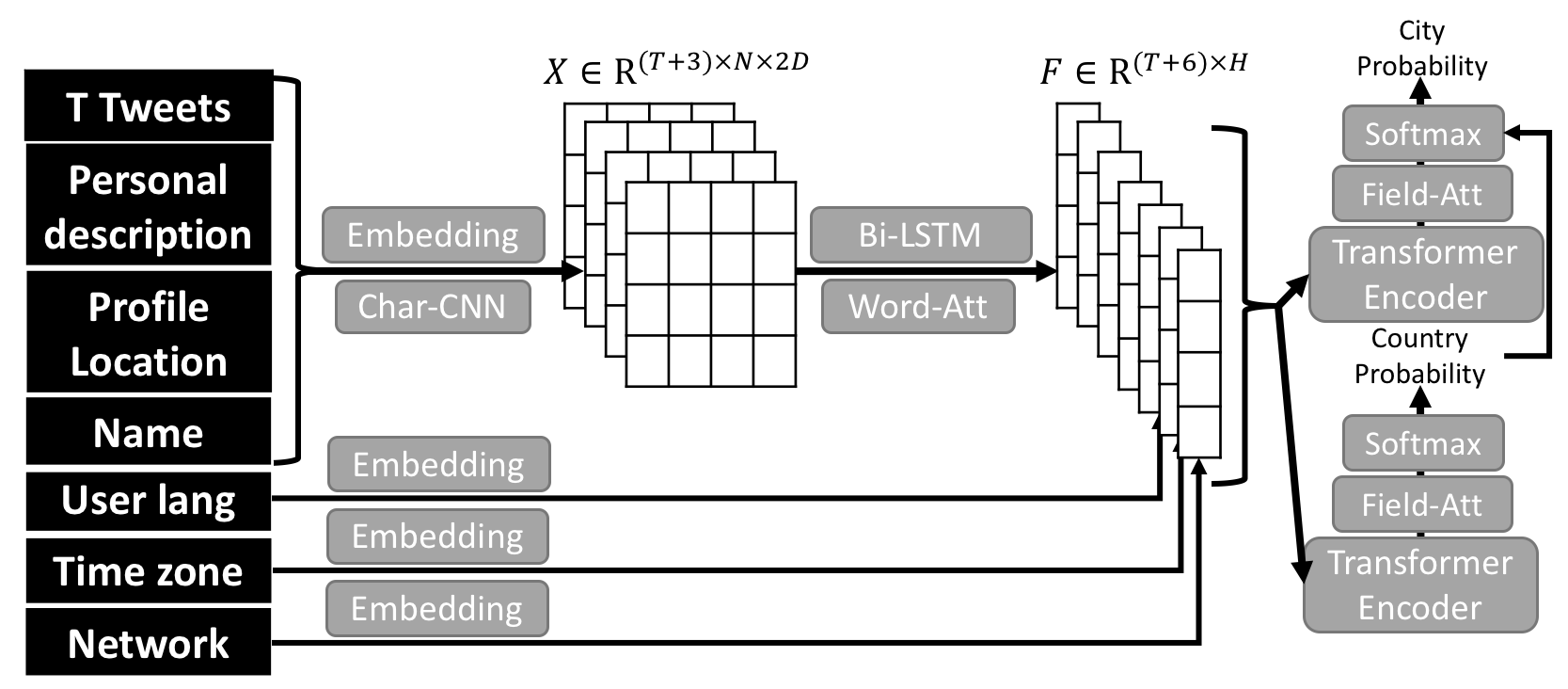
The overall architecture of our hierarchical location prediction model is shown in Figure 1. It first maps four text features into a word embedding space. A bidirectional LSTM (Bi-LSTM) neural network Hochreiter and Schmidhuber (1997) is used to extract location-specific features from these text embedding vectors. Following Bi-LSTM, we use a word-level attention layer to generate representation vectors for these text fields. Combining all the text representations, a user language embedding, a timezone embedding, and a network embedding, we apply several layers of transformer encoders Vaswani et al. (2017) to learn the correlation among all the feature fields. The probability for each country is computed after a field-level attention layer. Finally, we use the country probability as a constraint for the city-level location prediction. We elaborate details of our model in the following sections.
3.1 Word Embedding
Assume one user has tweets, there are text fields for this user including personal description, profile location, and name. We first map each word in these text fields into a low dimensional embedding space. The embedding vector for word is computed as , where denotes vector concatenation. is the word-level embedding retrieved directly from an Embedding matrix by a lookup operation, where is the vocabulary size, and is the word-level embedding dimension. is a character-level word embedding that is generated from a character-level convolutional layer. Using character-level word embeddings is helpful for dealing with out-of-vocabulary tokens and overcoming the noisy nature of tweet text.
The character-level word embedding generation process is as follows. For a character in the word , we map it into a character embedding space and get a vector . In the convolutional layer, each filter generates a feature vector , where . is a bias term, and “” denotes element-wise inner product between and character window . After this convolutional operation, we use a max-pooling operation to select the most representative feature . With such filters, we get the character-level word embedding .
3.2 Text Representation
After the word embedding layer, every word in these texts are transformed into a dimension vector. Given a text with word sequence , we get a word embedding matrix from the embedding layer. We then apply a Bi-LSTM neural network to extract high-level semantic representations from text embedding matrices.
At every time step , a forward LSTM takes the word embedding of word and previous state as inputs, and generates the current hidden state . A backward LSTM reads the text from to and generates another state sequence. The hidden state for word is the concatenation of and . Concatenating all the hidden states, we get a semantic matrix
Because not all words in a text contribute equally towards location prediction, we further use a multi-head attention layer Vaswani et al. (2017) to generate a representation vector for each text. There are attention heads that allow the model to attend to important information from different representation subspaces. Each head computes a text representation as a weighted average of these word hidden states. The computation steps in a multi-head attention layer are as follows.
where is an attention context vector learned during training, , and are projection parameters, . An attention head first projects the attention context and the semantic matrix into query and key subspaces by , respectively. The matrix product between query and key after softmax normalization is an attention weight that indicates important words among the projected value vectors . Concatenating heads together, we get one representation vector after projection by for each text field.
3.3 Feature Fusion
For two categorical features, we assign an embedding vector with dimension for each time zone and language. These embedding vectors are learned during training. We pretrain network embeddings for users involved in the mention network using LINE Tang et al. (2015). Network embeddings are fixed during training. We get a feature matrix by concatenating text representations of text fields, two embedding vectors of categorical features, and one network embedding vector.
We further use several layers of transformer encoders Vaswani et al. (2017) to learn the correlation between different feature fields. Each layer consists of a multi-head self-attention network and a feed-forward network (FFN). One transformer encoder layer first uses input feature to attend important information in the feature itself by a multi-head attention sub-layer. Then a linear transformation sub-layer is applied to each position identically. Similar to Vaswani et al. (2017), we employ residual connection He et al. (2016) and layer normalization Ba et al. (2016) around each of the two sub-layers. The output of the first transformer encoder layer is generated as follows.
where , , and .
Since there is no position information in the transformer encoder layer, our model cannot distinguish between different types of features, eg. tweet text and personal description. To overcome this issue, we add feature type embeddings to the input representations . There are seven features in total. Each of them has a learned feature type embedding with dimension so that one feature type embedding and the representation of the corresponding feature can be summed.
Because the input and the output of transformer encoder have the same dimension, we stack layers of transformer encoders to learn representations for country-level prediction and city-level prediction respectively. These two sets of encoders share the same input , but generate different representations and for country and city predictions.
The final classification features for country-level and city-level location predictions are the row-wise weighted average of and . Similar to the word-level attention, we use a field-level multi-head attention layer to select important features from vectors and fuse them into a single vector.
where are two attention context vectors.
| Twitter-US | Twitter-World | WNUT | |||||||||
| Train | Dev. | Test | Train | Dev. | Test | Train | Dev. | Test | |||
| # users | 429K | 10K | 10K | 1.37M | 10K | 10K | 742K | 7.46K | 10K | ||
|
228K | 5.32K | 5.34K | 917K | 6.50K | 6.48K | 742K | 7.46K | 10K | ||
| # tweets | 36.4M | 861K | 831K | 11.2M | 488K | 315K | 8.97M | 90.3K | 99.7K | ||
|
84.60 | 86.14 | 83.12 | 8.16 | 48.83 | 31.59 | 12.09 | 12.10 | 9.97 | ||
3.4 Hierarchical Location Prediction
The final probability for each country is computed by a softmax function
where is a linear projection parameter, is a bias term, and is the number of countries.
After we get the probability for each country, we further use it to constrain the city-level prediction
where is a linear projection parameter, is a bias term, and is the number of cities. is the country-city correlation matrix. If city belongs to country , then is , otherwise . is a penalty term learned during training. The larger of , the stronger of the country constraint. In practise, we also experimented with letting the model learn the country-city correlation matrix during training, which yields similar performance.
We minimize the sum of two cross-entropy losses for country-level prediction and city-level prediction.
where and are one-hot encodings of city and country labels. is the weight to control the importance of country-level supervision signal. Since a large would potentially interfere with the training process of city-level prediction, we just set it as in our experiments. Tuning this parameter on each dataset may further improve the performance.
4 Experiment Settings
4.1 Datasets
To validate our method, we use three widely adopted Twitter location prediction datasets. Table 1 shows a brief summary of these three datasets. They are listed as follows.
Twitter-US is a dataset compiled by Roller et al. (2012). It contains 429K training users, 10K development users, and 10K test users in North America. The ground truth location of each user is set to the first geotag of this user in the dataset. We assign the closest city to each user’s ground truth location using the city category built by Han et al. (2012). Since this dataset only covers North America, we change the first level location prediction from countries to administrative regions (eg. state or province). The administrative region for each city is obtained from the original city category.
Twitter-World is a Twitter dataset covering the whole world, with 1,367K training users, 10K development users, and 10K test users Han et al. (2012). The ground truth location for each user is the center of the closest city to the first geotag of this user. Only English tweets are included in this dataset, which makes it more challenging for a global-level location prediction task.
We downloaded these two datasets from Github 222https://github.com/afshinrahimi/geomdn. Each user in these two datasets is represented by the concatenation of their tweets, followed by the geo-coordinates. We queried Twitter’s API to add user metadata information to these two datasets in February 2019. We only get metadata for about 53% and 67% users in Twitter-US and Twitter-World respectively. Because of Twitter’s privacy policy change, we could not get the time zone information anymore at the time of collection.
WNUT was released in the 2nd Workshop on Noisy User-generated Text Han et al. (2016). The original user-level dataset consists of 1 million training users, 10K users in development set and test set each. Each user is assigned with the closest city center as the ground truth label. Because of Twitter’s data sharing policy, only tweet IDs of training and development data are provided. We have to query Twitter’s API to reconstruct the training and development dataset. We finished our data collection around August 2017. About 25% training and development users’ data cannot be accessed at that time. The full anonymized test data is downloaded from the workshop website 333https://noisy-text.github.io/2016/geo-shared-task.html.
4.2 Text Preprocessing & Network Construction
For all the text fields, we first convert them into lower case, then use a tweet-specific tokenizer from NLTK444https://www.nltk.org/api/nltk.tokenize.html to tokenize them. To keep a reasonable vocabulary size, we only keep tokens with frequencies greater than 10 times in our word vocabulary. Our character vocabulary includes characters that appear more than 5 times in the training corpus.
We construct user networks from mentions in tweets. For WNUT, we keep users satisfying one of the following conditions in the mention network: (1) users in the original dataset (2) users who are mentioned by two different users in the dataset. For Twitter-US and Twitter-World, following previous work Rahimi et al. (2018), a uni-directional edge is set if two users in our dataset directly mentioned each other, or they co-mentioned another user. We remove celebrities who are mentioned by more than 10 different users from the mentioning network. These celebrities are still kept in the dataset and their network embeddings are set as 0.
4.3 Evaluation Metrics
We evaluate our method using four commonly used metrics listed below.
Accuracy: The percentage of correctly predicted home cities.
Acc@161: The percentage of predicted cities which are within a 161 km (100 miles) radius of true locations to capture near-misses.
Median: The median distance measured in kilometer from the predicted city to the true location coordinates.
Mean: The mean value of error distances in predictions.
4.4 Hyperparameter Settings
In our experiments, we initialize word embeddings with released 300-dimensional Glove vectors Pennington et al. (2014). For words not appearing in Glove vocabulary, we randomly initialize them from a uniform distribution U(-0.25, 0.25). We choose the character embedding dimension as 50. The character embeddings are randomly initialized from a uniform distribution U(-1.0,1.0), as well as the timezone embeddings and language embeddings. These embeddings are all learned during training. Because our three datasets are sufficiently large to train our model, the learning is quite stable and performance does not fluctuate a lot.
Network embeddings are trained using LINE Tang et al. (2015) with parameters of dimension 600, initial learning rate 0.025, order 2, negative sample size 5, and training sample size 10000M. Network embeddings are fixed during training. For users not appearing in the mention network, we set their network embedding vectors as .
| Twitter-US | Twitter-World | WNUT | |||
|---|---|---|---|---|---|
| Batch size | 32 | 64 | 64 | ||
| Initial learning rate | |||||
|
300 | 300 | 300 | ||
|
50 | 50 | 50 | ||
|
3,4,5 | 3,4,5 | 3,4,5 | ||
|
100 | 100 | 100 | ||
| : number of heads | 10 | 10 | 10 | ||
|
3 | 3 | 3 | ||
| : initial penalty term | 1 | 1 | 1 | ||
|
1 | 1 | 1 | ||
|
2400 | 2400 | 2400 | ||
|
100 | 50 | 20 |
| Twitter-US | Twitter-World | WNUT | ||||||||
| Acc@161 | Median | Mean | Acc@161 | Median | Mean | Accuracy | Acc@161 | Median | Mean | |
| Text | ||||||||||
| Wing and Baldridge (2014) | 49.2 | 170.5 | 703.6 | 32.7 | 490.0 | 1714.6 | - | - | - | - |
| Rahimi et al. (2015b)* | 50 | 159 | 686 | 32 | 530 | 1724 | - | - | - | - |
| Miura et al. (2017)-TEXT | 55.6 | 110.5 | 585.1 | - | - | - | 35.4 | 50.3 | 155.8 | 1592.6 |
| Rahimi et al. (2017) | 55 | 91 | 581 | 36 | 373 | 1417 | - | - | - | - |
| HLPNN-Text | 57.1 | 89.92 | 516.6 | 40.1 | 299.1 | 1048.1 | 37.3 | 52.9 | 109.3 | 1289.4 |
| Text+Meta | ||||||||||
| Miura et al. (2017)-META | 67.2 | 46.8 | 356.3 | - | - | - | 54.7 | 70.2 | 0 | 825.8 |
| HLPNN-Meta | 61.1 | 64.3 | 454.8 | 56.4 | 86.2 | 762.1 | 57.2 | 73.1 | 0 | 572.5 |
| Text+Net | ||||||||||
| Rahimi et al. (2015a)* | 60 | 78 | 529 | 53 | 111 | 1403 | - | - | - | - |
| Rahimi et al. (2017) | 61 | 77 | 515 | 53 | 104 | 1280 | - | - | - | - |
| Miura et al. (2017)-UNET | 61.5 | 65 | 481.5 | - | - | - | 38.1 | 53.3 | 99.9 | 1498.6 |
| Do et al. (2017) | 66.2 | 45 | 433 | 53.3 | 118 | 1044 | - | - | - | - |
| Rahimi et al. (2018)-MLP-TXT+NET | 66 | 56 | 420 | 58 | 53 | 1030 | - | - | - | - |
| Rahimi et al. (2018)-GCN | 62 | 71 | 485 | 54 | 108 | 1130 | - | - | - | - |
| HLPNN-Net | 70.8 | 31.6 | 361.5 | 58.9 | 59.9 | 827.6 | 37.8 | 53.3 | 105.26 | 1297.7 |
| Text+Meta+Net | ||||||||||
| Miura et al. (2016) | - | - | - | - | - | - | 47.6 | - | 16.1 | 1122.3 |
| Jayasinghe et al. (2016) | - | - | - | - | - | - | 52.6 | - | 21.7 | 1928.8 |
| Miura et al. (2017) | 70.1 | 41.9 | 335.7 | - | - | - | 56.4 | 71.9 | 0 | 780.5 |
| HLPNN | 72.7 | 28.2 | 323.1 | 68.4 | 6.20 | 610.0 | 57.6 | 73.4 | 0 | 538.8 |
A brief summary of hyperparameter settings of our model is shown in Table 2. The initial learning rate is . If the validation accuracy on the development set does not increase, we decrease the learning rate to and train the model for additional 3 epochs. Empirically, training terminates within 10 epochs. Penalty is initialized as and is adapted during training. We apply dropout on the input of Bi-LSTM layer and the output of two sub-layers in transformer encoders with dropout rate 0.3 and 0.1 respectively. We use the Adam update rule Kingma and Ba (2014) to optimize our model. Gradients are clipped between -1 and 1. The maximum numbers of tweets per user for training and evaluating on Twitter-US are 100 and 200 respectively. We only tuned our model, learning rate, and dropout rate on the development set of WNUT.
5 Results
5.1 Baseline Comparisons
In our experiments, we evaluate our model under four different feature settings: Text, Text+Meta, Text+Network, Text+Meta+Network. HLPNN-Text is our model only using tweet text as input. HLPNN-Meta is the model that combines text and metadata (description, location, name, user language, time zone). HLPNN-Net is the model that combines text and mention network. HLPNN is our full model that uses text, metadata, and mention network for Twitter user geolocation.
We present comparisons between our model and previous work in Table 3. As shown in the table, our model outperforms these baselines across three datasets under various feature settings.
Only using text feature from tweets, our model HLPNN-Text works the best among all these text-based location prediction systems and wins by a large margin. It not only improves prediction accuracy but also greatly reduces mean error distance. Compared with a strong neural model equipped with local dialects Rahimi et al. (2017), it increases Acc@161 by an absolute value 4% and reduces mean error distance by about 400 kilometers on the challenging Twitter-World dataset, without using any external knowledge. Its mean error distance on Twitter-World is even comparable to some methods using network feature Do et al. (2017).
With text and metadata, HLPNN-Meta correctly predicts locations of 57.2% users in WNUT dataset, which is even better than these location prediction systems that use text, metadata, and network. Because in the WNUT dataset the ground truth location is the closest city’s center, Our model achieves 0 median error when its accuracy is greater than 50%. Note that Miura et al. (2017) used 279K users added with metadata in their experiments on Twitter-US, while we use all 449K users for training and evaluation, and only 53% of them have metadata, which makes it difficult to make a fair comparison.
Adding network feature further improves our model’s performances. It achieves state-of-the-art results combining all features on these three datasets. Even though unifying network information is not the focus of this paper, our model still outperforms or has comparable results to some well-designed network-based location prediction systems like Rahimi et al. (2018). On Twitter-US dataset, our model variant HLPNN-Net achieves a 4.6% increase in Acc@161 against previous state-of-the-art methods Do et al. (2017) and Rahimi et al. (2018). The prediction accuracy of HLPNN-Net on WNUT dataset is similar to Miura et al. (2017), but with a noticeable lower mean error distance.
5.2 Ablation Study
In this section, we provide an ablation study to examine the contribution of each model component. Specifically, we remove the character-level word embedding, the word-level attention, the field-level attention, the transformer encoders, and the country supervision signal one by one at a time. We run experiments on the WNUT dataset with text features.
| Accuracy | Acc@161 | Median | Mean | |
|---|---|---|---|---|
| HLPNN | 37.3 | 52.9 | 109.3 | 1289.4 |
| w/o Char-CNN | 36.3 | 51.0 | 130.8 | 1429.9 |
| w/o Word-Att | 36.4 | 51.5 | 130.2 | 1377.5 |
| w/o Field-Att | 37.0 | 52.0 | 121.8 | 1337.5 |
| w/o encoders | 36.8 | 52.5 | 117.4 | 1402.9 |
| w/o country | 36.7 | 52.6 | 124.8 | 1399.2 |
The performance breakdown for each model component is shown in Table 4. Compared to the full model, we can find that the character-level word embedding layer is especially helpful for dealing with noisy social media text. The word-level attention also provides performance gain, while the field-level attention only provides a marginal improvement. The reason could be the multi-head attention layers in the transformer encoders already captures important information among different feature fields. These two transformer encoders learn the correlation between features and decouple these two level predictions. Finally, using the country supervision can help model to achieve a better performance with a lower mean error distance.
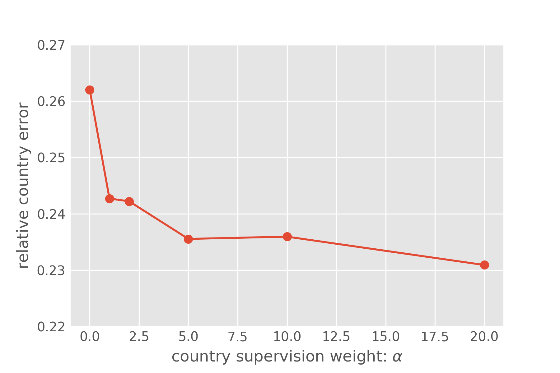
5.3 Country Effect
To directly measure the effect of adding country-level supervision, we define a relative country error which is the percentage of city-level predictions located in incorrect countries among all misclassified city-level predictions.
The lower this metric means the better one model can predict the city-level location, at least in the correct country.
We vary the weight of country-level supervision signal in our loss function from 0 to 20. The larger means the more important the country-level supervision during the optimization. When equals 0, there is no country-level supervision in our model. As shown in Figure 2, increasing would improve the relative country error from 26.2% to 23.1%, which shows the country-level supervision signal indeed can help our model predict the city-level location towards the correct country. This possibly explains why our model has a lower mean error distance when compared to other methods.
6 Conclusion
In this paper, we propose a hierarchical location prediction neural network, which combines text, metadata, network information for user location prediction. Our model can accommodate various feature combinations. Extensive experiments have been conducted to validate the effectiveness of our model under four different feature settings across three commonly used benchmarks. Our experiments show our HLPNN model achieves state-of-the-art results on these three datasets. It not only improves the prediction accuracy but also significantly reduces the mean error distance. In our ablation analysis, we show that using character-aware word embeddings is helpful for overcoming noise in social media text. The transformer encoders effectively learn the correlation between different features and decouple the two different level predictions. In our experiments, we also analyzed the effect of adding country-level regularization. The country-level supervision could effectively guide the city-level prediction towards the correct country, and reduce the errors where users are misplaced in the wrong countries.
Though our HLPNN model achieves great performances under Text+Net and Text+Meta+Net settings, potential improvements could be made using better graph-level classification frameworks. We currently only use network information to train network embeddings as user-level features. For future work, we would like to explore ways to combine graph-level classification methods and our user-level learning model. Propagating features from connected friends would provide much more information than just using network embedding vectors. Besides, our model assumes each post of one user all comes from one single home location but ignores the dynamic user movement pattern like traveling. We plan to incorporate temporal states to capture location changes in future work.
Acknowledgments
This work was supported in part by the Office of Naval Research (ONR) N0001418SB001 and N000141812108. The views and conclusions contained in this document are those of the authors and should not be interpreted as representing the official policies, either expressed or implied, of the ONR.
References
- Amitay et al. (2004) Einat Amitay, Nadav Har’El, Ron Sivan, and Aya Soffer. 2004. Web-a-where: geotagging web content. In Proceedings of the 27th annual international ACM SIGIR conference on Research and development in information retrieval, pages 273–280. ACM.
- Ba et al. (2016) Jimmy Lei Ba, Jamie Ryan Kiros, and Geoffrey E Hinton. 2016. Layer normalization. arXiv preprint arXiv:1607.06450.
- Backstrom et al. (2010) Lars Backstrom, Eric Sun, and Cameron Marlow. 2010. Find me if you can: improving geographical prediction with social and spatial proximity. In Proceedings of the 19th international conference on World wide web, pages 61–70. ACM.
- Berggren et al. (2016) Max Berggren, Jussi Karlgren, Robert Östling, and Mikael Parkvall. 2016. Inferring the location of authors from words in their texts. arXiv preprint arXiv:1612.06671.
- Bilhaut et al. (2003) Frédérik Bilhaut, Thierry Charnois, Patrice Enjalbert, and Yann Mathet. 2003. Geographic reference analysis for geographic document querying. In Proceedings of the HLT-NAACL 2003 workshop on Analysis of geographic references-Volume 1, pages 55–62. Association for Computational Linguistics.
- Buyukokkten et al. (1999) Orkut Buyukokkten, Junghoo Cho, Hector Garcia-Molina, Luis Gravano, and Narayanan Shivakumar. 1999. Exploiting geographical location information of web pages.
- Carley et al. (2016) Kathleen M Carley, Momin Malik, Peter M Landwehr, Jürgen Pfeffer, and Michael Kowalchuck. 2016. Crowd sourcing disaster management: The complex nature of twitter usage in padang indonesia. Safety science, 90:48–61.
- Do et al. (2017) Tien Huu Do, Duc Minh Nguyen, Evaggelia Tsiligianni, Bruno Cornelis, and Nikos Deligiannis. 2017. Multiview deep learning for predicting twitter users’ location. arXiv preprint arXiv:1712.08091.
- Earle et al. (2012) Paul S Earle, Daniel C Bowden, and Michelle Guy. 2012. Twitter earthquake detection: earthquake monitoring in a social world. Annals of Geophysics, 54(6).
- Ebrahimi et al. (2018) Mohammad Ebrahimi, Elaheh ShafieiBavani, Raymond Wong, and Fang Chen. 2018. A unified neural network model for geolocating twitter users. In Proceedings of the 22nd Conference on Computational Natural Language Learning, pages 42–53.
- Graham et al. (2014) Mark Graham, Scott A Hale, and Devin Gaffney. 2014. Where in the world are you? geolocation and language identification in twitter. The Professional Geographer, 66(4):568–578.
- Han et al. (2012) Bo Han, Paul Cook, and Timothy Baldwin. 2012. Geolocation prediction in social media data by finding location indicative words. Proceedings of COLING 2012, pages 1045–1062.
- Han et al. (2013) Bo Han, Paul Cook, and Timothy Baldwin. 2013. A stacking-based approach to twitter user geolocation prediction. In Proceedings of the 51st Annual Meeting of the Association for Computational Linguistics: System Demonstrations, pages 7–12.
- Han et al. (2016) Bo Han, Afshin Rahimi, Leon Derczynski, and Timothy Baldwin. 2016. Twitter geolocation prediction shared task of the 2016 workshop on noisy user-generated text. In Proceedings of the 2nd Workshop on Noisy User-generated Text (WNUT), pages 213–217.
- He et al. (2016) Kaiming He, Xiangyu Zhang, Shaoqing Ren, and Jian Sun. 2016. Deep residual learning for image recognition. In Proceedings of the IEEE conference on computer vision and pattern recognition, pages 770–778.
- Hecht et al. (2011) Brent Hecht, Lichan Hong, Bongwon Suh, and Ed H Chi. 2011. Tweets from justin bieber’s heart: the dynamics of the location field in user profiles. In Proceedings of the SIGCHI conference on human factors in computing systems, pages 237–246. ACM.
- Hochreiter and Schmidhuber (1997) Sepp Hochreiter and Jürgen Schmidhuber. 1997. Long short-term memory. Neural computation, 9(8):1735–1780.
- Hong et al. (2012) Liangjie Hong, Amr Ahmed, Siva Gurumurthy, Alexander J Smola, and Kostas Tsioutsiouliklis. 2012. Discovering geographical topics in the twitter stream. In Proceedings of the 21st international conference on World Wide Web, pages 769–778. ACM.
- Huang and Carley (2017) Binxuan Huang and Kathleen M Carley. 2017. On predicting geolocation of tweets using convolutional neural networks. In International Conference on Social Computing, Behavioral-Cultural Modeling and Prediction and Behavior Representation in Modeling and Simulation, pages 281–291. Springer.
- Huang and Carley (2018) Binxuan Huang and Kathleen M Carley. 2018. Location order recovery in trails with low temporal resolution. IEEE Transactions on Network Science and Engineering.
- Huang and Carley (2019) Binxuan Huang and Kathleen M Carley. 2019. A large-scale empirical study of geotagging behavior on twitter. In Proceedings of the 2019 IEEE/ACM International Conference on Advances in Social Networks Analysis and Mining 2019. ACM.
- Jayasinghe et al. (2016) Gaya Jayasinghe, Brian Jin, James Mchugh, Bella Robinson, and Stephen Wan. 2016. Csiro data61 at the wnut geo shared task. In Proceedings of the 2nd Workshop on Noisy User-generated Text (WNUT), pages 218–226.
- Kingma and Ba (2014) Diederik P Kingma and Jimmy Ba. 2014. Adam: A method for stochastic optimization. arXiv preprint arXiv:1412.6980.
- Mahmud et al. (2012) Jalal Mahmud, Jeffrey Nichols, and Clemens Drews. 2012. Where is this tweet from? inferring home locations of twitter users. In Sixth International AAAI Conference on Weblogs and Social Media.
- Miura et al. (2016) Yasuhide Miura, Motoki Taniguchi, Tomoki Taniguchi, and Tomoko Ohkuma. 2016. A simple scalable neural networks based model for geolocation prediction in twitter. In Proceedings of the 2nd Workshop on Noisy User-generated Text (WNUT), pages 235–239.
- Miura et al. (2017) Yasuhide Miura, Motoki Taniguchi, Tomoki Taniguchi, and Tomoko Ohkuma. 2017. Unifying text, metadata, and user network representations with a neural network for geolocation prediction. In Proceedings of the 55th Annual Meeting of the Association for Computational Linguistics (Volume 1: Long Papers), volume 1, pages 1260–1272.
- Miyazaki et al. (2018) Taro Miyazaki, Afshin Rahimi, Trevor Cohn, and Timothy Baldwin. 2018. Twitter geolocation using knowledge-based methods. In Proceedings of the 2018 EMNLP Workshop W-NUT: The 4th Workshop on Noisy User-generated Text, pages 7–16.
- Overell (2009) Simon E Overell. 2009. Geographic information retrieval: Classification, disambiguation and modelling. Ph.D. thesis, Citeseer.
- Pennington et al. (2014) Jeffrey Pennington, Richard Socher, and Christopher Manning. 2014. Glove: Global vectors for word representation. In Proceedings of the 2014 conference on empirical methods in natural language processing (EMNLP), pages 1532–1543.
- Qian et al. (2017) Yujie Qian, Jie Tang, Zhilin Yang, Binxuan Huang, Wei Wei, and Kathleen M Carley. 2017. A probabilistic framework for location inference from social media. arXiv preprint arXiv:1702.07281.
- Quercia et al. (2010) Daniele Quercia, Neal Lathia, Francesco Calabrese, Giusy Di Lorenzo, and Jon Crowcroft. 2010. Recommending social events from mobile phone location data. In 2010 IEEE international conference on data mining, pages 971–976. IEEE.
- Rahimi et al. (2018) Afshin Rahimi, Trevor Cohn, and Tim Baldwin. 2018. Semi-supervised user geolocation via graph convolutional networks. arXiv preprint arXiv:1804.08049.
- Rahimi et al. (2015a) Afshin Rahimi, Trevor Cohn, and Timothy Baldwin. 2015a. Twitter user geolocation using a unified text and network prediction model. arXiv preprint arXiv:1506.08259.
- Rahimi et al. (2017) Afshin Rahimi, Trevor Cohn, and Timothy Baldwin. 2017. A neural model for user geolocation and lexical dialectology. arXiv preprint arXiv:1704.04008.
- Rahimi et al. (2015b) Afshin Rahimi, Duy Vu, Trevor Cohn, and Timothy Baldwin. 2015b. Exploiting text and network context for geolocation of social media users. arXiv preprint arXiv:1506.04803.
- Roller et al. (2012) Stephen Roller, Michael Speriosu, Sarat Rallapalli, Benjamin Wing, and Jason Baldridge. 2012. Supervised text-based geolocation using language models on an adaptive grid. In Proceedings of the 2012 Joint Conference on Empirical Methods in Natural Language Processing and Computational Natural Language Learning, pages 1500–1510. Association for Computational Linguistics.
- Sakaki et al. (2010) Takeshi Sakaki, Makoto Okazaki, and Yutaka Matsuo. 2010. Earthquake shakes twitter users: real-time event detection by social sensors. In Proceedings of the 19th international conference on World wide web, pages 851–860. ACM.
- Tang et al. (2015) Jian Tang, Meng Qu, Mingzhe Wang, Ming Zhang, Jun Yan, and Qiaozhu Mei. 2015. Line: Large-scale information network embedding. In Proceedings of the 24th international conference on world wide web, pages 1067–1077. International World Wide Web Conferences Steering Committee.
- Vaswani et al. (2017) Ashish Vaswani, Noam Shazeer, Niki Parmar, Jakob Uszkoreit, Llion Jones, Aidan N Gomez, Łukasz Kaiser, and Illia Polosukhin. 2017. Attention is all you need. In Advances in Neural Information Processing Systems, pages 5998–6008.
- Wing and Baldridge (2014) Benjamin Wing and Jason Baldridge. 2014. Hierarchical discriminative classification for text-based geolocation. In Proceedings of the 2014 conference on empirical methods in natural language processing (EMNLP), pages 336–348.
- Wing and Baldridge (2011) Benjamin P Wing and Jason Baldridge. 2011. Simple supervised document geolocation with geodesic grids. In Proceedings of the 49th annual meeting of the association for computational linguistics: Human language technologies-volume 1, pages 955–964. Association for Computational Linguistics.
- Zhang et al. (2017) Yu Zhang, Wei Wei, Binxuan Huang, Kathleen M Carley, and Yan Zhang. 2017. Rate: Overcoming noise and sparsity of textual features in real-time location estimation. In Proceedings of the 2017 ACM on Conference on Information and Knowledge Management, pages 2423–2426. ACM.