Heat dissipation rate in a nonequilibrium viscoelastic medium

Abstract

A living non-Newtonian matter like the cell cortex and tissues are driven out-of-equilibrium at multiple spatial and temporal scales. The stochastic dynamics of a particle embedded in such a medium are non-Markovian, given by a generalized Langevin equation. Due to the non-Markovian nature of the dynamics, the heat dissipation and the entropy production rate cannot be computed using the standard methods for Markovian processes. In this work, to calculate heat dissipation, we use an effective Markov description of the non-Markovian dynamics, which includes the degrees-of-freedom of the medium. Specifically, we calculate entropy production and heat dissipation rate for a spherical colloid in a non-Newtonian medium whose rheology is given by a Maxwell viscoelastic element in parallel with a viscous fluid element, connected to different temperature baths. This problem is nonequilibrium for two reasons: the medium is nonequilibrium due to different effective temperatures of the bath, and the particle is driven out-of-equilibrium by an external stochastic force. When the medium is nonequilibrium, the effective non-Markov dynamics of the particle may lead to a negative value of heat dissipation and entropy production rate. The positivity is restored when the medium’s degree-of-freedom is considered. When the medium is at equilibrium, and the only nonequilibrium component is the external driving, the correct dissipation is obtained from the effective description of the particle.

• November 2019

1 Introduction

Active systems are a subclass of nonequilibrium systems that are driven out of equilibrium at a microscopic scale [1, 2]. They are maintained in a nonequilibrium steady state (NESS) by a constant input of energy. The NESS is characterized by a positive entropy production rate (EPR) [3, 4, 5, 6, 7] and violation of the fluctuation dissipation relation (FDR) [8, 9]. For a Markovian dynamics, there are multiple equivalent approaches to compute the EPR [6, 7]. For instance, the EPR and heat dissipation rate (HDR) in the linear response regime can be computed using the Harda-Sasa relation [8, 10]; this shows the relation between HDR and the violation of FDR.

In recent years, much attention has been given to the calculation of the HDR and EPR in various active systems[11, 12, 13, 14, 15, 16, 17]. One model is particularly well studied: the stochastic thermodynamics of active particles driven by an Ornstein-Uhlenbeck process [18, 19, 20, 21, 22]. Similarly, a passive particle embedded in a suspension of active Brownian particles can also be modeled as a particle driven by an Ornstein-Uhlenbeck process [23, 24], and the corresponding HDR can be calculated using the standard methods [22, 25]. The HDR thus calculated is the excess dissipation due to the passive particle in addition to the basal HDR due to the active particles in the suspension. In the above-mentioned cases, the active component is the fluctuating force driving the particles. This is justified for a dilute suspension but not for a dense suspension, for which the rheology is non-Newtonian. The study of passive particles driven by active fluctuations and embedded in a non-Newtonian medium has been much less studied [26]; the stochastic thermodynamics of such complex systems has received even less attention [27].

In general, the rheology of living and non-living active matter is non-Newtonian [2, 28, 29]. Moreover, these systems are driven out-of-equilibrium by processes operating at multiple spatial and temporal scales [11, 30, 31, 29]. For instance, the cell cortex, in specific contexts, can be modeled as a Maxwell fluid with the relaxation time depending on the factors like cross-linker turnover rate, actin polymerization, and depolarization rate [32, 33]. At a larger scale, the fluidity of tissues is governed by T1 transitions regulated by the activity of actomyosin [34, 35]. Most of these processes are nonequilibrium. This makes it different from a passive non-Newtonian matter, where the complex rheology is a result of relaxation at multiple timescales that do not consume energy [36, 28]. The dynamics of a passive particle embedded in such a non-Newtonian medium is necessarily non-Markovian, requiring a careful analysis to estimate the corresponding HDR and EPR.

As a start toward understanding this difficult topic, we ask the question: what is the HDR and EPR due to a passive particle embedded in such a nonequilibrium non-Newtonian medium? To answer this question, we study the HDR and EPR of a spherical colloid embedded in a complex medium comprising of a stochastic Maxwell viscoelastic element [37, 38] in parallel to a viscous fluid element (see Fig. 1 (A)), with an external fluctuating force acting on it. The fluctuations in the two elements are taken to be Gaussian white noise from two different temperature baths. The stochastic dynamics of the colloid is given by a generalized Langevin equation (GLE). The non-Markovian GLE can be represented by an equivalent Markovian dynamics. Using this Markov dynamics and the Harda-Sasa relation, we obtain the corresponding HDR and EPR.

In Ref. [27], a generalization of Harada-Sasa relation for a particle in a non-Newtonian medium is proposed. We find that the results in Ref. [27] are only true when the non-Newtonian medium is passive, i.e., the fluctuations are thermal. To calculate the HDR of a particle in a nonequilibrium medium, it is necessary to include the medium’s dissipative degrees-of-freedom (DOF) along with that of the particle’s DOF. Ignoring the medium’s DOF may, erroneously, lead to a negative EPR. This work aids in understanding the dissipation in non-Markovian systems in general, for which it has been shown that the EPR is negative [39, 40, 41, 42].

In the following, first, we briefly outline the derivation of the Langevin dynamics of the particle starting from the stress equations of the medium and then calculate the HDR for the GLE using an effective Markov description. We then summarize the limits in which the particle’s dynamics as proposed in ref. [27] leads to the correct dissipation.

2 Passive particle in an active viscoelastic medium

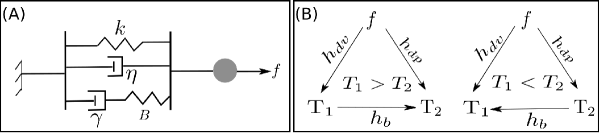
Figure 1: (A) Schematic of a particle in a viscoelastic medium driven by a fluctuating force $f$. The viscoelastic medium is a viscous element of viscosity $\eta$ and corresponding fluctuation due to an effective bath at temperature $T_{1}$, in parallel to a Maxwell viscoelastic element of elastic modulus $B$, viscosity $\gamma$ and corresponding fluctuation due to an effective bath at temperature $T_{2}$. (B) Schematic of heat flow between the different fluctuation sources. $h_{dv}$ is the heat flow from the external driving to $T_{1}$ and $h_{dp}$ is the heat flow from the external driving to $T_{2}$. The heat flow between the two temperature baths $T_{1}$ and $T_{2}$ is $h_{b}$. For $T_{1}>T_{2}$, the heat flow is from $T_{1}$ to $T_{2}$ and $h_{b}<0$, for $T_{1}<T_{2}$ the heat flow is opposite and $h_{b}>0$.

Consider the viscoelastic medium to be an active gel [2] modeled as a two-component viscoelastic material. The viscous component is water, and the actomyosin is modeled as a Maxwell viscoelastic element, where the relaxation time is given by the turnover of actomyosin [33]. The stress fluctuations of water are thermal, and the temperature is $T_{1}$. The active gel is out-of-equilibrium; hence, the fluctuation-dissipation relation is not satisfied [43]. In general, the active stress fluctuations will be correlated in space and time. For simplicity, we take the active fluctuation, at the timescale of interest, to be Gaussian white noise, characterized by an effective temperature $T_{2}$. In this setup the medium is passive when $T_{2}=T_{1}$. The schematic of this viscoelastic medium is shown in Fig. 1 (A), consisting of a Maxwell viscoelastic element and a viscous fluid element in parallel . The total stress in the medium is

$$\sigma_{ij}=-p\,\delta_{ij}+\sigma^{1}_{ij}+\sigma^{2}_{ij},$$ (1)

where $p$ is the pressure and $\sigma^{1}_{ij}$ and $\sigma^{2}_{ij}$ are the symmetric traceless parts of the stress tensor due to the viscous and Maxwell viscoelastic element respectively. The viscous stress is given by [44]

$$\sigma^{1}_{ij}=\eta\left(\partial_{i}v_{j}+\partial_{j}v_{i}\right)+\vartheta^{1}_{ij},$$ (2)

where $\eta$ is the viscosity, $v$ is the velocity, and $\vartheta^{1}_{ij}$ is the stochastic component of the stress due to the temperature bath $T_{1}$. The Maxwell stress $\sigma_{ij}^{2}$ is given by [43]

$$\left(\sigma^{2}_{ij}+\tau\partial_{t}\sigma^{2}_{ij}\right)=\gamma\left(\partial_{j}v_{i}+\partial_{i}v_{j}\right)+\vartheta^{2}_{ij},$$ (3)

where $\tau=\gamma/B$ is the Maxwell relaxation time, $B$ is the elastic modulus, $\gamma$ is the viscosity, and $\vartheta^{2}_{ij}$ is the stochastic component of the stress due to the temperature bath $T_{2}$. The variance of the stochastic component of the stresses is

$$\langle\vartheta^{\alpha}_{ij}(x,t)\vartheta_{kl}^{\alpha}(x^{\prime},t^{\prime})\rangle=2\Lambda_{\alpha}\delta({x-x^{\prime}})\delta(t-t^{\prime})\left[\delta_{ik}\delta_{jl}+\delta_{il}\delta_{jk}-\frac{2}{3}\delta_{ij}\delta_{kl}\right],\,\quad$$ (4)

where $\alpha\in(1,2)$, $\Lambda_{1}=T_{1}\eta$, and $\Lambda_{2}=T_{2}\gamma$. The incomprehensibility condition is $\nabla\cdot v=0$ and the dynamics in the Stokes limit is $\nabla\cdot\sigma=0$. As mentioned before, for the actomyosin system, $T_{1}$ is the real temperature, and $T_{2}$ is the effective temperature given by the active stress fluctuations. For simplicity, we have taken the active stress fluctuation to be isotropic Gaussian white noise; however, in general, it can be asymmetric and colored [43, 45]. In Fourier space Eq. 1 reads (through the text we denote the Fourier transform of function $\phi(t)$ as $\tilde{\phi}(\omega)=\int_{-\infty}^{\infty}dt\phi(t)e^{-i\omega t}$)

$$\tilde{\sigma}_{ij}(\omega)=-p\,\delta_{ij}+\left(\frac{\gamma}{-i\omega\tau+1}+\eta\right)(\partial_{i}\tilde{v}_{j}+\partial_{j}\tilde{v}_{i})+\tilde{\vartheta}^{1}_{ij}+\frac{1}{-i\omega\tau+1}\tilde{\vartheta}^{2}_{ij}.$$

The stochastic dynamics of a spherical colloidal particle of radius $a$ embedded in this medium is obtained by integrating the stress in Eq. 2 over the surface of the sphere and using a no-slip boundary condition. This yields the GLE (see appendix of ref. [45] for derivation)

$$-\omega^{2}m\tilde{x}-i\omega\gamma(\omega)\tilde{x}=-k\tilde{x}+\tilde{f}+\tilde{\xi}_{1}+\tilde{\xi}_{2},$$ (5)

where $m$ is the mass of the particle, $k$ is the stiffness of the external harmonic confinement, $f$ is the external stochastic force applied on the particle, $\tilde{\xi}_{1}$ is zero mean Gaussian white noise with correlation $\langle\tilde{\xi}_{1}(\omega)\tilde{\xi}_{1}(\omega^{\prime})\rangle=2T_{1}\gamma_{1}\delta(\omega+\omega^{\prime})$, $\tilde{\xi}_{2}$ is zero mean Gaussian noise with correlation $\langle\tilde{\xi}_{2}(\omega)\tilde{\xi}_{2}(\omega^{\prime})\rangle=2T_{2}\gamma_{2}\delta(\omega+\omega^{\prime})/(\omega^{2}\tau^{2}+1)$, and the frequency dependent friction coefficient

$$\gamma(\omega)=\left(\gamma_{1}+\frac{\gamma_{2}}{-i\omega\tau+1}\right),$$ (6)

where $\gamma_{1}=6\pi\eta a$ and $\gamma_{2}=6\pi\gamma a$. Note that the external force $f$ can represent external driving, for instance, by a fluctuating optical trap [46, 47], as well as fluctuation due to active stresses localized at the particle [26]. In the time domain Eq. 5 reads

$$m\ddot{x}+\frac{\gamma_{2}}{\tau}\int_{-\infty}^{t}dt^{\prime}\,e^{-(t-t^{\prime})/\tau}\dot{x}+\gamma_{1}\dot{x}=-kx+f+\xi_{1}+\xi_{2},$$ (7)

where $\xi_{1}$ and $\xi_{2}$ are noise sources either active or thermal with correlations $\langle\xi_{2}(t)\xi_{2}(t^{\prime})\rangle=2T_{2}\gamma_{2}e^{-(t-t^{\prime})/\tau}/\tau$ and $\langle\xi_{1}(t)\xi_{1}(t^{\prime})\rangle=2T_{1}\gamma_{1}\delta(t-t^{\prime})$, and $f$ is an external fluctuating force with correlation $\langle f(t)f(t^{\prime})\rangle=2\Lambda_{n}e^{-(t-t^{\prime})/\tau_{n}}/\tau_{n}$. The correlation function is defined as

$$C_{\dot{x}\dot{x}}(t)=\langle(\dot{x}(t)-\langle\dot{x}\rangle)(\dot{x}(0)-\langle\dot{x}\rangle)\rangle,$$ (8)

and the response function is defined by the relation [9]

$$\langle\dot{x}(t)\rangle_{\epsilon}-\langle\dot{x}\rangle=\epsilon\int_{-\infty}^{t}\chi_{\dot{x}}(t-t^{\prime})f_{p}(t^{\prime})dt^{\prime},$$ (9)

where $\langle\cdot\rangle_{\epsilon}$ denotes the average over the steady state with small perturbation $\epsilon f_{p}(t)$ and $\langle\cdot\rangle$ denotes the average for $\epsilon=0$. The dynamics given by Eq. 7 is out of equilibrium when the fluctuation dissipation relation is not satisfied, i.e.,

$$\tilde{C}_{\dot{x}\dot{x}}(\omega)\neq 2T\tilde{\chi}^{\prime}_{\dot{x}}(\omega).$$ (10)

where $T$ is the temperature of the thermal bath, $\tilde{\chi}^{\prime}_{\dot{x}}(\omega)$ is the real component of the response function. The equilibrium limit is obtained when fluctuations $\xi_{1}$ and $\xi_{2}$ are thermal, i.e., $T_{1}=T_{2}=T$12 and $\Lambda_{n}=0$. In the following, we calculate the EPR and HDR at NESS when the system is out of equilibrium.

3 Entropy production rate

For the stochastic dynamics given by

$$\gamma_{i}\dot{x}_{i}=f_{i}+\xi_{i},$$ (11)

where $i\in(1,...,N)$, and $\xi_{i}$ is a Gaussian noise with correlation $\langle\xi_{i}(t)\xi_{j}(t^{\prime})\rangle=2T_{i}\gamma_{i}\delta_{ij}\delta(t-t^{\prime})$, $\gamma_{i}$ is the friction coefficient, and $f_{i}$ is force on the variable $i$, using the Harada-Sasa relation the heat dissipated by variable $i$ is given by [8, 10]

$$h_{i}=\gamma_{i}\langle\dot{x}_{i}\rangle^{2}+\gamma_{i}\int_{-\infty}^{\infty}\frac{d\omega}{2\pi}\left(\tilde{C}_{\dot{x}_{i}\dot{x}_{i}}(\omega)-2T_{i}\tilde{\chi}^{\prime}_{\dot{x}_{i}}(\omega)\right).$$ (12)

The total HDR (h) and the EPR (s) is

$$h=\sum_{i=1}^{N}h_{i}\quad\mathrm{and}\quad s=\sum_{i=1}^{N}\frac{h_{i}}{T_{i}}.$$ (13)

At equilibrium $T_{i}=T$ and $\tilde{C}_{\dot{x}_{i}\dot{x}_{i}}=2T\tilde{\chi}_{i}^{\prime}(\omega)$, for which $h_{i}=0$. In ref. [27] an expression for computing heat dissipation rate for the equation

$$\int_{-\infty}^{t}dt^{\prime}\,\gamma(t-t^{\prime})\dot{x}(t^{\prime})=-k\,x(t)+\xi(t),$$ (14)

where $i\in(1,...,N)$ was proposed by generalizing the Harada-Sasa relation to

$$h_{\mathrm{NM}}=\int_{-\infty}^{\infty}\frac{d\omega}{2\pi}\tilde{\gamma}_{i}^{\prime}(\omega)\left(\tilde{C}_{\dot{x}\dot{x}}(\omega)+\langle\dot{x}\rangle^{2}-2T\tilde{\chi}^{\prime}_{\dot{x}}(\omega)\right),$$ (15)

where $\tilde{\gamma}^{\prime}(\omega)$ is the real component of the friction and $T$ is the temperature of the bath. We now calculate the heat dissipation using Eq. 15 for the dynamics given by Eq. 5. From Eq. 6 we get

$$\gamma^{\prime}(\omega)=\gamma_{1}+\frac{\gamma_{2}}{\omega^{2}\tau^{2}+1}.$$ (16)

The response function as defined by Eq. 9 for the dynamics in Eq. 5 is $\tilde{\chi}_{\dot{x}}(\omega)=-i\omega/\Gamma(\omega)$, where

$$\Gamma(\omega)=\left(k-\omega^{2}m-\frac{i\gamma_{2}\omega}{-i\omega\tau+1}-i\omega\gamma_{1}\right),$$ (17)

from which we get its real component as

$$\tilde{\chi}_{\dot{x}}^{\prime}=\frac{\omega^{2}}{|\Gamma(\omega)|^{2}}\left(\frac{\gamma_{2}}{\omega^{2}\tau^{2}+1}+\gamma_{1}\right).$$ (18)

The spectrum of the correlation function as defined in Eq. 8 for the dynamics in Eq. 5 is

$$\tilde{C}_{\dot{x}\dot{x}}(\omega)=\frac{\omega^{2}}{|\Gamma(\omega)|^{2}}\left(2T_{1}\gamma_{1}+\frac{2\Lambda_{n}}{\omega^{2}\tau_{n}^{2}+1}+\frac{2T_{2}\gamma_{2}}{\omega^{2}\tau^{2}+1}\right).$$ (19)

In overdamped limit, without external confinement ($k=0$), and fluctuating force ($\Lambda_{n}=0$), the two viscosities and temperatures can be estimated experimentally from the correlation $\tilde{C}_{\dot{x}\dot{x}}(\omega)$ and the response $\tilde{\chi}_{\dot{x}}$ measured using microrheology techniques [48, 49]. The two viscosities can be read from $|\tilde{\chi}_{\dot{x}}|^{2}$ which saturates to $1/(\gamma_{1}+\gamma_{2})$ at low frequencies and $1/\gamma_{1}$ at high frequencies. Knowing the viscosities, the two temperatures can be calculated from the low and high frequency limits of $\tilde{C}_{\dot{x}\dot{x}}(\omega)/|\tilde{\chi}_{\dot{x}}|^{2}$.

Substituting Eq. 18 and Eq. 19 in Eq. 15 and taking $T=T_{1}$ gives

$$h_{\mathrm{NM}}=\int_{-\infty}^{\infty}\frac{d\omega}{2\pi}\frac{2\omega^{2}\gamma^{\prime}(\omega)}{|\Gamma(\omega)|^{2}}\left(\frac{\Lambda_{n}}{\omega^{2}\tau_{n}^{2}+1}+\frac{\gamma_{2}(T_{2}-T_{1})}{\omega^{2}\tau^{2}+1}\right).$$ (20)

The integrand can be negative for $T_{1}>T_{2}$ which will lead to negative HDR and EPR. In this framework, it is not possible to explain negative EPR. In the following, we show that, in general, Eq. 15 does not lead to the correct expression for HDR and EPR. As shown in the following text, it leads to the correct result only when the viscoelastic medium is passive, i.e., $T_{1}=T_{2}$.

The GLE in Eq. 7 is non-Markovian. To analyze the HDR and EPR we need an equivalent Markov representation. The Markovian dynamics corresponding to Eq. 7 can be obtained by defining

$$p=\frac{\gamma_{2}}{\tau}\int_{-\infty}^{t}dt^{\prime}\,e^{-(t-t^{\prime})/\tau}\dot{x}.$$ (21)

Using this substitution we get the following Markov dynamics corresponding to Eq. 7:

$$m\dot{v} = -p-\gamma_{1}v-kx+f+\xi_{1},$$ (22)

$$\dot{x} = v,$$ (23)

$$\tau\dot{p} = -p+\gamma_{2}v+\xi_{2},$$ (24)

$$\tau_{n}\dot{f} = -f+\xi_{n},$$ (25)

where $\xi_{1}$, $\xi_{2}$, and $\xi_{n}$ are zero mean Gaussian white noise of variance $2T_{1}\gamma_{1}$, $2T_{2}\gamma_{2}$, and $2\Lambda_{n}$ respectively. We emphasize that the variable $p$ is not just a convenient representation but has a physical interpretation as the force on the particle due to the Maxwell stress in Eq. 3, i.e.,

$$p_{i}(t)=\int_{\partial V}dS_{j}\,\sigma^{2}_{ij}(x,t),$$ (26)

where $\partial V$ is the surface of the particle. Hence, this representation is unique and justifies the noise source $\xi_{2}$ in Eq. 24.

For a Markovian dynamics, the HDR and EPR can be obtained using different methods [5, 7, 6], here, we use the Harda-Sasa relation in Eq. 12. The total dissipation is the sum of dissipation due to variables $v$ and $p$. Using Eq. 12 the dissipation corresponding to $v$ is

$$h_{v}=\gamma_{1}\int_{-\infty}^{\infty}\frac{d\omega}{2\pi}\left(\tilde{C}_{vv}(\omega)-2T_{1}\tilde{\chi}_{v}^{\prime}(\omega)\right),$$ (27)

where $T_{1}$ is the temperature of the bath corresponding to friction coefficient $\gamma_{1}$. The dissipation corresponding to variable $p$ is

$$h_{p}=\frac{1}{\gamma_{2}}\int_{-\infty}^{\infty}\frac{d\omega}{2\pi}\left(\tilde{C}_{pp}(\omega)-2T_{2}\tilde{\chi}_{p}^{\prime}(\omega)\right),$$ (28)

where $\tilde{C}_{pp}=\langle p^{2}(\omega)\rangle-\langle p(\omega)\rangle^{2}$ is the correlation function, $\tilde{\chi}_{p}=\langle\delta p\rangle/\delta f_{p}$ is the response function. Notice that $\gamma_{2}$ is in the denominator, $\gamma_{2}$ is the mobility corresponding to variable $p$. The entropy production rate is

$$s=\frac{h_{v}}{T_{1}}+\frac{h_{p}}{T_{2}}.$$ (29)

Substituting Eq. 18 and Eq. 19 in Eq. 27 we get

$$h_{v}=h_{b}+h_{dv},$$ (30)

where the heat flow between the temperature bath $T_{1}$ and $T_{2}$ is

$$h_{b}=\int_{-\infty}^{\infty}\frac{d\omega}{2\pi}\frac{\omega^{2}}{|\Gamma(\omega)|^{2}}\frac{2\gamma_{1}\gamma_{2}(T_{2}-T_{1})}{\omega^{2}\tau^{2}+1},$$ (31)

and the heat flow from the driving force $f$ to the bath $T_{1}$ is

$$h_{dv}=\int_{-\infty}^{\infty}\frac{d\omega}{2\pi}\frac{\omega^{2}}{|\Gamma(\omega)|^{2}}\frac{2\Lambda_{n}\gamma_{1}}{\omega^{2}\tau_{n}^{2}+1}.$$ (32)

From Eq. 22 to 25 we get

$$\tilde{p}(\omega)=-\frac{i\omega\gamma_{2}\left(\tilde{y}(\omega)+\xi_{1}(\omega)\right)}{\Gamma(\omega)(-i\omega\tau+1)}+\frac{\left(k-\omega^{2}m-i\omega\gamma_{1}\right)}{\Gamma(\omega)(-i\omega\tau+1)}\tilde{\xi}_{2}.$$ (33)

The corresponding correlation spectrum reads

$$\tilde{C}_{pp}=\frac{1}{|\Gamma(\omega)|^{2}(\omega^{2}\tau^{2}+1)} \left[\omega^{2}\gamma_{2}^{2}\left(2T_{1}\gamma_{1}+\frac{2\Lambda_{n}}{\omega^{2}\tau^{2}_{n}+1}\right)\right.$$ (34)

$$\left.+\left((k-\omega^{2}m)^{2}+\omega^{2}\gamma_{1}^{2}\right)2T_{2}\gamma_{2}\right],$$

and the response function reads

$$\chi_{p}=\frac{\gamma_{2}\left(k-\omega^{2}m-i\omega\gamma_{1}\right)}{\Gamma(\omega)(-i\omega\tau+1)}.$$ (35)

The real component of this response function is

$$\chi^{\prime}_{p}=\frac{\gamma_{2}\left((k-\omega^{2}m)^{2}+\omega^{2}\gamma_{1}(\gamma_{2}+\gamma_{1})\right)}{|\Gamma(\omega)|^{2}(\omega^{2}\tau^{2}+1)}.$$ (36)

Substituting Eq. 36 and Eq. 34 into Eq. 28 we get

$$h_{p}=-h_{b}+h_{dp},$$ (37)

where $h_{b}$ is given by Eq. 31 and the heat flow from the driving force $f$ to the bath $T_{2}$ is

$$h_{dp}=\int_{-\infty}^{\infty}\frac{d\omega}{2\pi}\frac{1}{|\Gamma(\omega)|^{2}}\frac{2\Lambda_{n}\gamma_{2}\omega^{2}}{(\omega^{2}\tau^{2}_{n}+1)(\omega^{2}\tau^{2}+1)}.$$ (38)

Fig. 1 (B) show the direction of heat flow between different baths. The heat flow is from the driving $f$ to the two baths $T_{1}$ and $T_{2}$ although $T_{2}$ and $f$ are not directly connected. The heat flow between the baths $T_{1}$ and $T_{2}$ is from “hotter” to “colder”.

The EPR as obtained by substituting Eq. 31,32,and 38 in Eq. 29 is

$$s=\left(\frac{T_{2}-T_{1}}{T_{1}T_{2}}\right)h_{b}+\frac{h_{dv}}{T_{1}}+\frac{h_{dp}}{T_{2}}.$$ (39)

The first term on the right is quadratic in the temperature difference, hence, as expected, the EPR is always positive. The total heat dissipated is

$$h=h_{v}+h_{p}=h_{dv}+h_{dp},$$ (40)

which is always positive for $\Lambda_{n}\neq 0$. We now compare this with Eq. 20. For $T_{1}=T_{2}$, i.e., when the viscoelastic medium is passive, the total HDR obtained from Eq. 20 is equal to that given by Eq. 40 and the corresponding EPR is equal to that in Eq. 39. When $T_{1}\neq T_{2}$ the two expressions may lead to very different values. As mentioned before, for large enough temperature difference $(T_{1}-T_{2})$ the HDR as obtained in Eq. 20 and the corresponding EPR can be negative, whereas the HDR and EPR as given by Eq. 40 and Eq. 39 respectively are always positive.

4 Overdamped Limit

We now calculate the EPR and HDR in the overdamped limit of Eq. 7. This is obtained by simply setting $m\to 0$. In this limit Eq. 17 reduces to

$$\Gamma(\omega)=\frac{\gamma_{1}\tau(i\omega-\omega_{1})(i\omega-\omega_{2})}{(-i\omega\tau+1)},$$ (41)

where

$$\omega_{1,2}=\frac{(\gamma_{2}+\gamma_{1}+k\tau)\pm\sqrt{(\gamma_{2}+\gamma_{1}+k\tau)^{2}-4k\gamma_{1}\tau}}{2\gamma_{1}\tau}.$$

Substituting Eq. 41 in Eq. 31 and integrating we get

$$h_{b}=\frac{\gamma_{2}(T_{2}-T_{1})}{\tau(\gamma_{2}+\gamma_{1}+k\tau)}.$$ (42)

Substituting Eq. 41 in Eq. 38 and integrating gives

$$h_{dp}=\frac{\gamma_{2}\Lambda_{n}}{(\gamma_{1}\tau+\tau_{n}^{2}k+\tau_{n}(\gamma_{2}+\gamma_{1}+k\tau))(\gamma_{2}+\gamma_{1}+k\tau)}.$$ (43)

Similarly, substituting Eq. 41 in 32 we get

$$h_{dv}=\frac{\Lambda_{n}(\gamma_{1}\tau_{n}+\tau\tau_{n}k+\tau(\gamma_{2}+\gamma_{1}+k\tau))}{\tau_{n}(\gamma_{1}\tau+\tau_{n}^{2}k+\tau_{n}(\gamma_{2}+\gamma_{1}+k\tau))(\gamma_{2}+\gamma_{1}+k\tau)}.$$ (44)

The total HDR and EPR are obtained upon substitution of Eq. 43-44 and Eq. 42 in Eq. 40 and Eq. 39 respectively. To check the validity of the results we take the viscous limit of the Maxwell stress by taking $\tau\to 0$ and the medium to be passive ($T_{1}=T_{2}=T$). In this limit the dynamics in Eq.22 to 25 reduces to

$$(\gamma_{1}+\gamma_{2})\dot{x} = -kx+f+\sqrt{2T(\gamma_{1}+\gamma_{2})}\xi,$$ (45)

$$\tau_{n}\dot{f} = -f+\xi_{n}.$$ (46)

This is the dynamics of a particle in a Newtonian fluid of viscosity $\eta+\gamma$ driven by an Ornstein-Uhlenbeck process $f$. The EPR given by Eq. 39 reduces to

$$s=\frac{\Lambda_{n}}{T\tau_{n}(k\tau_{n}+(\gamma_{1}+\gamma_{2}))},$$ (47)

which is same as that obtained for this dynamics directly in different contexts[20, 21].

In absence on an external driving ($\Lambda_{n}=0$) $h_{dv}=h_{dp}=0$ and the total HDR $h=h_{b}$, the EPR from Eq. 39 is

$$s=\frac{(T_{1}-T_{2})^{2}}{T_{1}T_{2}}\frac{k_{2}^{2}}{(k_{2}\gamma_{1}+(k_{2}+k)\gamma_{2})},$$ (48)

where we have defined $k_{2}=6\pi\eta aB$ and substituted $\tau=\gamma/B$. The EPR increases with the increase in the elasticity of the Maxwell element but decreases with the increase in the elasticity of the external potential. The increase in viscosity of both Maxwell and viscous elements leads to a decrease in the EPR. In the absence of external harmonic potential, the EPR reduces to

$$s=\frac{(T_{1}-T_{2})^{2}}{T_{1}T_{2}}\frac{\gamma_{2}}{\tau(\gamma_{1}+\gamma_{2})}.$$ (49)

In the overdamped limit taking $\tau\to 0$ when $T_{1}\neq T_{2}$ leads to $h_{b}\to\infty$. To calculate this limit we need to include inertia, which adds a high frequency cutoff to the correlation function. Similarly, for $\tau_{n}\to 0$ the dissipation $h_{dv}\,\mathrm{and}\,h_{dp}\to\infty$. Again, to calculate this limit, we need to introduce a high-frequency cutoff, which for this case, is provided by inertial relaxation.

5 Discussion

In summary, we compute the heat dissipation and entropy production rate of a spherical particle suspended in a viscoelastic medium composed of a Maxwell fluid element and a viscous element in parallel driven by a stochastic force. The fluctuation corresponding to the viscosities of the fluid ($\eta$) and the Maxwell element ($\gamma$) act as two effective temperature baths $T_{1}$ and $T_{2}$ respectively. The dynamics of the particle is given by a generalized Langevin equation which is non-Markovian. This problem is nonequilibrium for two reasons: the effective temperature of the baths may be unequal, and the particle is driven by an external stochastic force.

To calculate the heat dissipation and the entropy production rate for this case, we write an effective Markov description of the non-Markovian dynamics. This is done by explicitly including the relaxation dynamics of the Maxwell fluid along with the particle dynamics. For this effective Markov description, we compute the dissipation using the Harada-Sasa relation. We find that the equation for heat dissipation rate proposed in ref. [27], and that obtained in this work are different. The results match only when the medium is passive ($T_{1}=T_{2}$), and the only nonequilibrium input is the fluctuating force. A particle in a viscoelastic medium driven by a fluctuating force is realized experimentally in ref. [50]. In this system, the medium is passive, and the only nonequilibrium component is the driving force on the particle. Hence, for this system, it is possible to calculate HDR using Eq. 15. However, for a similar experiment when the medium is active Eq. 15 cannot be used, and a more detailed analysis of the kind proposed in this paper is required.

It has been shown that non-Markovian dynamics can lead to a negative EPR [39, 40, 41, 42]. We show that indeed when the mediums degree-of-freedom is not included, the EPR can be negative for some values of the parameters. However, if all the relevant degrees of freedom are included, the dynamics are Markovian, and the EPR is always positive.

This approach is useful when the microscopic stress model is known. However, in general, the microscopic model for the medium is not experimentally accessible. For instance, using active and passive microrheology techniques, the correlation and response function of the embedded particle can be obtained. From this, inferring the equilibrium and nonequilibrium degrees of freedom of the medium may not be possible. One of the useful directions for the future will be to explore the limits in which the correct Markov description can be inferred from microrheology data. In recent years progress has been made in quantifying the nonequilibrium dynamics through noninvasive approaches. In specific scenarios, the phase space current can be estimated from the real-space trajectories of particles [30, 51, 52]. In the future, it would be of interest to extend these approaches to active viscoelastic systems of the likes described in this paper.

6 Acknowledgments

ASV thanks Ananyo Maitra and Samuel Bell for insightful discussions and critical reading of the manuscript. This work has received support under the program “Investissements d’Avenir” launched by the French Government and implemented by ANR with the references ANR-10-LABX-0038 and ANR-10-IDEX-0001-02 PSL.

7 References

References

- [1] Ramaswamy S. The Mechanics and Statistics of Active Matter. Annu Rev Condens Matter Phys. 2010;1(1):323–345.
- [2] Marchetti MC, Joanny JF, Ramaswamy S, Liverpool TB, Prost J, Rao M, et al. Hydrodynamics of soft active matter. Rev Mod Phys. 2013;85(3):1143–1189.
- [3] Ge H, Qian M, Qian H. Stochastic theory of nonequilibrium steady states. Part II: Applications in chemical biophysics. Phys Rep. 2012;510(3):87–118.
- [4] Zhang XJ, Qian H, Qian M. Stochastic theory of nonequilibrium steady states and its applications. Part I. Phys Rep. 2012;510(1-2):1–86.
- [5] Seifert U. Stochastic thermodynamics, fluctuation theorems and molecular machines. Reports Prog Phys. 2012;75(12):126001.
- [6] Esposito M, Van Den Broeck C. Three faces of the second law. I. Master equation formulation. Phys Rev E - Stat Nonlinear, Soft Matter Phys. 2010;82(1).
- [7] Van den Broeck C, Esposito M. Three faces of the second law. II. Fokker-Planck formulation. Phys Rev E. 2010;82(1).
- [8] Harada T, Sasa SI. Equality connecting energy dissipation with a violation of the fluctuation-response relation. Phys Rev Lett. 2005;95(13):130602.
- [9] Chaikin PM, Lubensky TC. Principles of condensed matter physics. vol. 1. Cambridge university press Cambridge; 2000.
- [10] Harada T, Sasa SI. Energy dissipation and violation of the fluctuation-response relation in nonequilibrium Langevin systems. Phys Rev E - Stat Nonlinear, Soft Matter Phys. 2006;73(2).
- [11] Gnesotto FS, Mura F, Gladrow J, Broedersz CP. Broken detailed balance and non-equilibrium dynamics in living systems: A review. Reports Prog Phys. 2018;81(6).
- [12] Seara DS, Yadav V, Linsmeier I, Tabatabai AP, Oakes PW, Tabei SMA, et al. Entropy production rate is maximized in non-contractile actomyosin. Nat Commun. 2018;9(1):4948.
- [13] Floyd C, Papoian GA, Jarzynski C. Quantifying dissipation in actomyosin networks. Interface Focus. 2019;9(3):20180078.
- [14] Nardini C, Fodor é, Tjhung E, van Wijland F, Tailleur J, Cates ME. Entropy production in field theories without time-reversal symmetry: Quantifying the non-equilibrium character of active matter. Phys Rev X. 2017;7(2):021007.
- [15] Ganguly C, Chaudhuri D. Stochastic thermodynamics of active Brownian particles. Physical Review E. 2013;88(3):032102.
- [16] Speck T. Stochastic thermodynamics for active matter. EPL (Europhysics Letters). 2016;114(3):30006.
- [17] Chakraborti S, Mishra S, Pradhan P. Additivity, density fluctuations, and nonequilibrium thermodynamics for active Brownian particles. Physical Review E. 2016;93(5):052606.
- [18] Marconi UMB, Puglisi A, Maggi C. Heat, temperature and Clausius inequality in a model from active Brownian particles. Sci Rep. 2017;7(1):1–16.
- [19] Fodor É, Nardini C, Cates ME, Tailleur J, Visco P, Van Wijland F. How Far from Equilibrium Is Active Matter? Phys Rev Lett. 2016;117(3):38103.
- [20] Prawar Dadhichi L, Maitra A, Ramaswamy S. Origins and diagnostics of the nonequilibrium character of active systems. J Stat Mech Theory Exp. 2018;2018(12):123201.
- [21] Shankar S, Cristina Marchetti M. Hidden entropy production and work fluctuations in an ideal active gas. Phys Rev E. 2018;98(2):020604.
- [22] Pietzonka P, Seifert U. Entropy production of active particles and for particles in active baths. J Phys A: Math Theor. 2017;51(1):01LT01.
- [23] Chen DTN, Lau AWC, Hough LA, Islam MF, Goulian M, Lubensky TC, et al. Fluctuations and rheology in active bacterial suspensions. Phys Rev Lett. 2007;99(14):148302.
- [24] Maggi C, Paoluzzi M, Pellicciotta N, Lepore A, Angelani L, Di Leonardo R. Generalized energy equipartition in harmonic oscillators driven by active baths. Phys Rev Lett. 2014;113(23):238303.
- [25] Chaki S, Chakrabarti R. Effects of active fluctuations on energetics of a colloidal particle: Superdiffusion, dissipation and entropy production. Phys A Stat Mech its Appl. 2019;530:121574.
- [26] Vandebroek H, Vanderzande C. Dynamics of a polymer in an active and viscoelastic bath. Physical Review E. 2015;92(6):060601.
- [27] Deutsch JM, Narayan O. Energy dissipation and fluctuation response for particles in fluids. Phys Rev E - Stat Nonlinear, Soft Matter Phys. 2006;74(2):26112.
- [28] Spagnolie SE. Complex fluids in biological systems. Springer; 2015.
- [29] Mizuno D, Tardin C, Schmidt CF, MacKintosh FC. Nonequilibrium mechanics of active cytoskeletal networks. Science (80- ). 2007;315(5810):370–373.
- [30] Battle C, Broedersz CP, Fakhri N, Geyer VF, Howard J, Schmidt CF, et al. Broken detailed balance at mesoscopic scales in active biological systems. Science (80- ). 2016;352(6285):604–607.
- [31] Turlier H, Fedosov DA, Audoly B, Auth T, Gov NS, Sykes C, et al. Equilibrium physics breakdown reveals the active nature of red blood cell flickering. Nat Phys. 2016;12(5):513–519.
- [32] Toyota T, Head DA, Schmidt CF, Mizuno D. Non-Gaussian athermal fluctuations in active gels. Soft Matter. 2011;7(7):3234–3239.
- [33] Salbreux G, Charras G, Paluch E. Actin cortex mechanics and cellular morphogenesis. Trends Cell Biol. 2012;22(10):536–545.
- [34] Lecuit T, Lenne PF. Cell surface mechanics and the control of cell shape, tissue patterns and morphogenesis. Nat Rev Mol Cell Biol. 2007;8(8):633–644.
- [35] Krajnc M, Dasgupta S, Ziherl P, Prost J. Fluidization of epithelial sheets by active cell rearrangements. Phys Rev E. 2018;98(2):22409.
- [36] Doi M, Edwards SF. The theory of polymer dynamics. vol. 73. oxford university press; 1988.
- [37] Bland DR. Theory of linear viscoelasticity. vol. 241. Courier Dover Publications; 2016.
- [38] Keunings R. Theory of Viscoelasticity: An Introduction. vol. 13. Elsevier; 1983.
- [39] Bylicka B, Tukiainen M, Chruściński D, Piilo J, Maniscalco S. Thermodynamic power of non-Markovianity. Sci Rep. 2016;6:27989.
- [40] Bhattacharya S, Misra A, Mukhopadhyay C, Pati AK. Exact master equation for a spin interacting with a spin bath: Non-Markovianity and negative entropy production rate. Phys Rev A. 2017;95(1):012122.
- [41] García-García R. Nonadiabatic entropy production for non-Markov dynamics. Phys Rev E - Stat Nonlinear, Soft Matter Phys. 2012;86(3):31117.
- [42] Strasberg P, Esposito M. Non-Markovianity and negative entropy production rates. Phys Rev E. 2019;99(1):12120.
- [43] Basu A, Joanny JF, Jülicher F, Prost J. Thermal and non-thermal fluctuations in active polar gels. Eur Phys J E. 2008;27(2):149–160.
- [44] Foster D. Hydrodynamic Fluctuations, Broken Symmetry, and Correlation Fluctuations. vol. 35. Addison-Wesley, Redwood City, CA; 1983.
- [45] Lau AWC, Lubensky TC. Fluctuating hydrodynamics and microrheology of a dilute suspension of swimming bacteria. Phys Rev E - Stat Nonlinear, Soft Matter Phys. 2009;80(1):11917.
- [46] Bérut A, Imparato A, Petrosyan A, Ciliberto S. Stationary and transient fluctuation theorems for effective heat fluxes between hydrodynamically coupled particles in optical traps. Phys Rev Lett. 2016;116(6):1–5.
- [47] Berut A, Petrosyan A, Ciliberto S. Energy flow between two hydrodynamically coupled particles kept at different effective temperatures. Epl. 2014;107(6):60004.
- [48] MacKintosh FC, Schmidt CF. Microrheology. Curr Opin Colloid Interface Sci. 1999;4(4):300–307.
- [49] Zia RN. Active and passive microrheology: theory and simulation. Annu Rev Fluid Mech. 2018;50:371–405.
- [50] Toyabe S, Sano M. Energy dissipation of a Brownian particle in a viscoelastic fluid. Phys Rev E - Stat Nonlinear, Soft Matter Phys. 2008;77(4):41403.
- [51] Mura F, Gradziuk G, Broedersz CP. Nonequilibrium scaling behavior in driven soft biological assemblies. Phys Rev Lett. 2018;121(3):038002.
- [52] Mura F, Gradziuk G, Broedersz CP. Mesoscopic non-equilibrium measures can reveal intrinsic features of the active driving. Soft Matter. 2019;15(40):8067–8076.